


Languages
Pages
Legal


Journal of Virological Methods, 9 ( 1984) 3 17-324
Elsevier
JVM 00349
317
METHODS FOR COMPARING SEQUENCE DATA SUCH AS RESTRICTION
ENDONUCLEASE MAPS OR NUCLEOTIDE SEQUENCES OF VIRAL
NUCLEIC ACID MOLECULES
ADRIAN GIBBS and FRANK FENNER
Research School of Biological Sciences and John Curiin School of Medical Research, Australian National
University, Canberra, A.C.T. 2601, Australia
(Accepted 30 July 1984)
Maps of restriction endonuclease sites in the DNA genomes of orthopoxviruses were compared by
computer classification methods. Data from such maps were recorded as qualitative binary information,
and gave closely similar dendrograms when different dissimilarity measures and sorting strategies were used
for the computations. A method for calculating dendrograms from small data sets, by ‘hand’, is described in
detail to assist those who do not have access to suitable computer programs. The same calculation strategy
gave useful classifications of partial nucieotide and amino acid sequences of orthomyxovirus haemaggIuti-
nins.
restriction endonuclease maps classification poxviruses orthomyxoviruses
INTRODUCTION
Restriction endonucleases cut DNA molecules at particular nucleotide sequences
that are usually palindromic and four or six nucleotides in length. By various means,
the positions of those sequences (restriction sites) within a DNA molecule may be
mapped. Statistical methods have been devised to use such maps to estimate the
evolutionary distance between two related DNAs or to estimate the sequence varia-
tion within populations of organisms; these methods have been reviewed by Kaplan
(1983).
Maps of restriction sites are useful for comparing viral DNAs, as was first shown for
the genomes of the orthopoxviruses by Wittek et al. (1977). There is a large centra1
region in their genomes that is common to all species and may be used to align their
maps unequivocally (Mackett and Archard, 1979). Other parts of the maps are more
variable, and it is difficult to obtain an overall view of the relatedness of several species
or isolates merely by inspecting their maps. We have therefore computed classifica-
tions of the maps to simplify the comparisons, and report these methods here.
0166-0934/84/$03.00 0 1984 Elsevier Science Publishers B.V.
318
RESULTS
Computer classifications
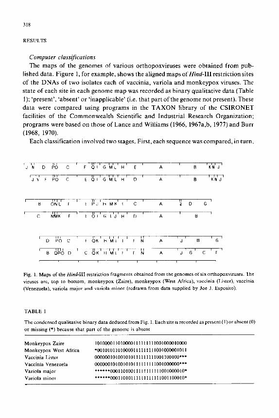
The maps of the genomes of various orthopoxviruses were obtained from pub-
lished data. Figure 1, for example, shows the aligned maps of Hind-III restriction sites
of the DNAs of two isolates each of vaccinia, variola and monkeypox viruses. The
state of each site in each genome map was recorded as binary qualitative data (Table
1); ‘present’, ‘absent’ or ‘inapplicable’ (i.e. that part of the genome not present). These
data were compared using programs in the TAXON library of the CSIRONET
facilities of the Commonwealth Scientific and Industrial Research Organization;
programs were based on those of Lance and Williams (1966, 1967a,b, 1977) and Burr
(1968, 1970).
Each classification involved two stages. First, each sequence was compared, in turn,
Fig. 1. Maps of the Hind-111 restriction fragments obtained from the genomes of six orthopoxviruses. The
viruses are, top to bottom, monkeypox (Zaire), monkeypox (West Africa), vaccinia (Lister), vaccinia
(Venezuela), variola major and variola minor (redrawn from data supplied by Joe J. Esposito).
TABLE 1
The condensed qualitative binary data deduced from Fig. 1, Each site is recorded as present (1) or absent (0)
or missing (*) because that part of the genome is absent
Monkeypox Zaire 10100001101000011
Monkeypox West Africa ‘0010101101000011
Vaccinia Lister 00000010100101011
Vaccinia Venezuela 00000010100101011
Variola major ******00011010011
Variola minor ******00011010111
111111001000010000
111111001000001011
111111001100100***
111111001000000***
11111111001000010*
11111111001100010*
319
with every other sequence and their similarity assessed using either the ‘squared Euclidean distance’ metric, which accentuates differences, or the ‘Canberra’ or ‘Cower’ metrics (Lance and Williams, 1967a), which do not. The similarities were recorded in a matrix, one matrix for each metric.
In the second stage of the classification, the matrices of similarities were reduced to dendrograms by the flexible agglomerative hierarchical classification method of Lance and Williams (1966, 1967b). For each classification thesortingstrategy wasused which had been shown to be most useful for that metric; the ‘minimum increment of sum of squares’ strategy (Burr, 1968, 1970) for ‘Euclidean’, and, for the others, ‘flexible strategy’, with parameters beta -0.25, alpha 0.125 and gamma 0 (Lance and Williams, 1967b).
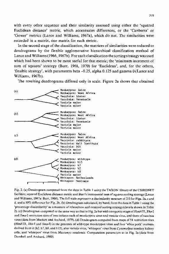
The resulting dendrograms differed only in scale. Figure 2a shows that obtained
(4 Monkeypox: wildtype Monkeypox: h15 Monkeypox: h7 Monkeypox: h2 Monkeypox: h8 Variola major Whitepox: Netherlands
r , WhFtepox: Mastomys ,
Fig. 2. (a) Dendrogram computed from the data in Table 1 using the TAXON library of the CSIRONET
facilities; squared Euclidean distance metric and Burr’s incremental sum of squares sorting strategy (Lance
and Williams, 1967a; Burr, 1968). The full scale represents a dissimilarity measure of 2.0 for Figs. 2a, c and
d, and a 50% difference for Fig. 2b. (b) Dendrogram calculated, by hand, from the data in Table 1 using the
‘percentage dissimilarity’ as a measure of relatedness and centroid sorting strategy (details shown in Table
2). (c) Dendrogram computed in the same way as that in Fig. 2a but with composite maps ofHind-III, X/IO-I
and Sma-I restriction sites of two isolates each of monkeypox virus and variola virus, and three of vaccinia
virus (data from Mackett and Archard, 1979). (d) Dendrogram computed from maps of 51 restriction sites
(Hind-III, Xho-I and Sma-I) in the genomes of wild-type monkeypox virus and four ‘white pock’ mutants
derived from it fh2, h7, h8, and h15), also variola virus, ‘whitepox’ virus from Cynomolgm monkey kidney
cells, and ‘whitepox’ virus from Musromys natdensis. Computation parameters as in Fig. 2a (data from
Dumbell and Archard, 1980).
320
using the squared Euclidean distance metric. It confirms the close relationship of each
pair of isolates, and suggests that vaccinia virus is more closely related to monkeypox
virus than to variola virus,
However, similar classifications of more detailed maps (66 restriction sites of
Hind-III, Xho-I and %a-I) of isolates of these viruses indicated (Fig. 2c) that
vaccinia may be slightly more closely related to variola than to monkeypox.
There may be several reasons for the difference in these results. For example, the
classification based on three enzymes (66 sites in all) might be expected to be more
accurate than that based on Hind-III alone (36 sites in all) because a greater propor-
tion of each genome was sampled. However, most Hind-III sites are in the central
conserved part of the genome (Mackett and Archard, 1979), and hence the Hind-III
map may be a better guide to the relatedness of the viruses than the mixed enzyme
map. Whatever the reason for the difference between these classifications, it is
important to realise that these methods are based on mutation data and therefore
assess close relationships more reliably than distant ones.
An example of the practical use of these methods is shown in Fig. 26, which is a
~lassi~~ation of the restriction maps of five monkeypox isolates, two ‘whitepox’
isolates and one variola isolate (Dumbell and Archard, 1980). Four of the monkeypox
isolates (h2, h7, h8, and h 15) were ‘white pock’ mutants isolated from the wild-type
monkeypox, and it can be seen that they group unequivocally with monkeypox virus
rather than with variola virus and the ‘whitepoxes’. The significance of this result is
that the ‘whitepoxes’ were thought to have been isolates from animals (‘Netherlands’
from ~ynorn~~gus monkey kidney cells: Gispen and Brand-Saathof, 1972; l ~us?o~ys’
from the kidney of a rat of that name shot in Zaire: Marennikova et al., 1976).
Subsequently, Marennikova et al. (1979) claimed that ‘whitepox’ viruses arose as
mutants of monkeypox virus, but Dumbell and Kapsenburg (1982) showed that the
Netherlands ‘whitepox’ isolate was a laboratory contaminant. The clustering of the
four ‘white pock’ mutants of monkeypox virus with the wild-type strain from which
they were isolated, and of both ‘whitepoxes’ with variola virus (Fig. 2d), indicates that
“whitepoxes’ are probably not ‘white pock’ mutants of monkeypox virus.
A non-computer method Not all people have access to computers, even fewer to the TAXON library of
CSIRONET, or similar programs in GENSTAT. However, it is quite simple to
calculate certain types of dendrograms from small sets of data like those in Table I
without the help of a computer.
The calculation is done in two stages. First, the dissimilarity of the maps is
calculated in some convenient way, for example, the matrix in Table 2 shows the
number of sites not shared by each pair of sequences expressed as a percentage of totai
number of sites in those sequences. Then the branching points of the dendrogram are
calculated in the following way. The matrix is inspected to find which pair of
sequences are most similar; sequences 5 and 6 in Table 2. This pair and its associated
321
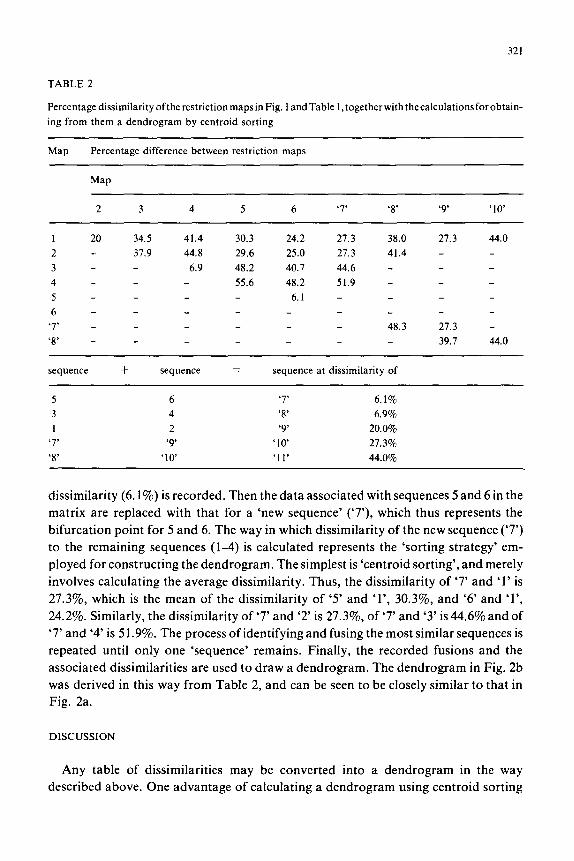
TABLE 2
PercentagedissimilarityoftherestrictionmapsinFig. landTable 1,togetherwith thecalculationsforobtain-
ing from them a dendrogram by centroid sorting
Map Percentage difference between restriction maps
Map
2 3 4 5 6 ‘7’ ‘8’ ‘9’ ‘10’
1 20 34.5 41.4 30.3 24.2 27.3 38.0 27.3 44.0
2 - 37.9 44.8 29.6 25.0 27.3 41.4 -
3 - - 6.9 48.2 40.7 44.6 -
4 - - 55.6 48.2 51.9 -
5 - - 6.1 -
6 - -
‘7’ _ - 48.3 27.3 -
‘8’ _ _ 39.7 44.0
sequence + sequence = sequence at dissimilarity of
5 6 ‘7’ 6.1%
3 4 ‘8’ 6.9%
1 2 ‘9’ 20.0%
‘7’ ‘9 ‘10 27.3%
‘8’ ‘10 ‘11’ 44.0%
dissimilarity (6.1%) is recorded. Then the data associated with sequences 5 and 6 in the
matrix are replaced with that for a ‘new sequence’ (‘7’), which thus represents the
bifurcation point for 5 and 6. The way in which dissimilarity of the new sequence (‘7’)
to the remaining sequences (l-4) is calculated represents the ‘sorting strategy’ em-
ployed for constructing the dendrogram. The simplest is ‘centroid sorting’, and merely
involves calculating the average dissimilarity. Thus, the dissimilarity of ‘7’ and ‘1’ is
27.3%, which is the mean of the dissimilarity of ‘5’ and ‘l’, 30.3%, and ‘6’ and ‘l’,
24.2%. Similarly, the dissimilarity of ‘7’ and ‘2’ is 27.3%, of ‘7’ and ‘3’ is 44.6% and of
‘7’ and ‘4’ is 5 1.9%. The process of identifying and fusing the most similar sequences is
repeated until only one ‘sequence’ remains. Finally, the recorded fusions and the
associated dissimilarities are used to draw a dendrogram. The dendrogram in Fig. 2b
was derived in this way from Table 2, and can be seen to be closely similar to that in
Fig. 2a.
DISCUSSION
Any table of dissimilarities may be converted into a dendrogram in the way
described above. One advantage of calculating a dendrogram using centroid sorting
322
AlNks/33 (N1NI) AIBHl35 IHlNl) Al PR/ 8134 (HINI) h/&1/42 (HlNl) b/USSR/90/77 (HlN1) A/Fort Warren/ 1150 (WlNl) AILoyanglb/57 (WINl) AiducklALbertaf 35J76 (HINl) A/suine/Iowaf 15130 (HlNi) A/New Jerseyill; JHINI) AfTokyoi 3167 (HZNZ) h/Netherlands/68 (HZN2) A/RI/ 5-157 (H2N2) A/Berkeley/ 68 (H2N2) A/dUCk/GDR/72 (H2N2) AJduckJAlbertal U/77 (N2N3) A/blue winged teai/604/78 (H2N3) A~~U~k~o~e~r~~~?7 {H2Nl) Afp~ntaillA1berrai293/17 (W2N9) AIduckiNew York!6750178 fW2N2) A/shearwater/Australia/75 (H5N3) Afshearwater/Australia/72 (WbNS) h/duck/ALbertaJ 1298179 (MNS) A/duck/Alberta/l297/79 (HbN9) A/tern/Australia/75 (HllN9) A~d~cki~~aine~~~b~ (KIlN9) Afd~~kf~~~l~~d~~6 fH1 IN6) Aldufkmew -fork/f2178 CHilN6) AiduckiMemphisj546176 (tiilN9) A/gullftiss/26/80 (B13N6) A/~ull/W704/77 (H13~6) A/turkey/Ontario/6118/68 (H8N4) Alduck/Alberraia27/78 IHBN4) AiducklAlbertai283i77 (uaw+) A~t~~ke~~~~~co~s~~~ I!66 (H9N2) A~d~~k~A~be~t~~6#~76 tHlZN5)
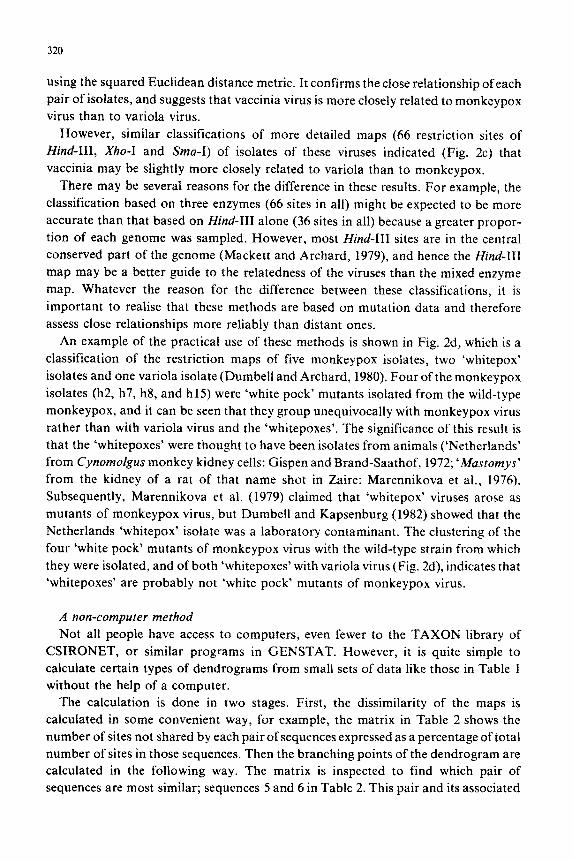
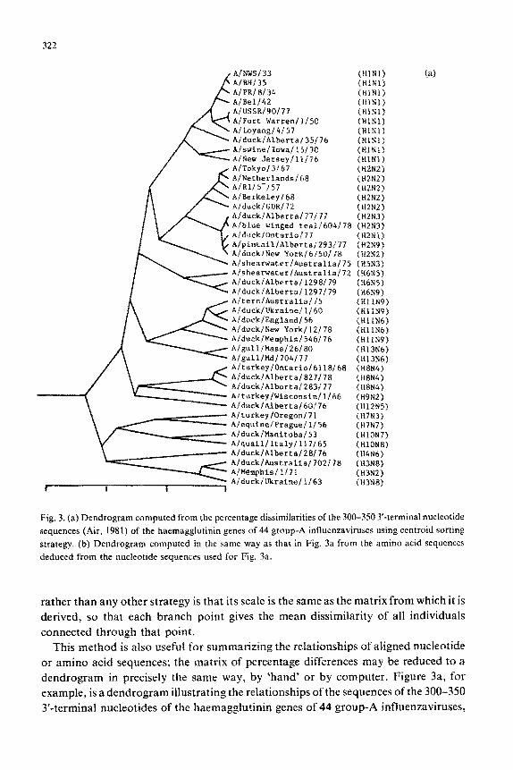
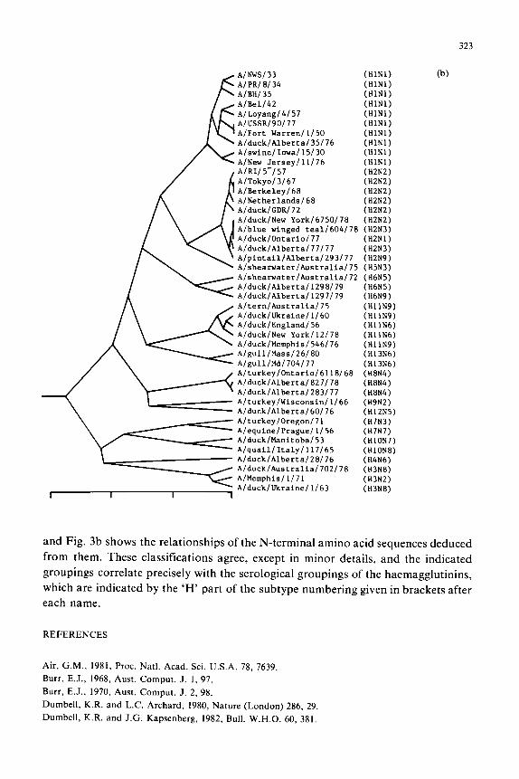
Fig. 3. (a) Dendrogram computed from the percentage dissimilarities of the 300-350 Y-terminal nucleotide
sequences (Air, 1981) of the haemagglutinin genes of 44 group-A influenzaviruses using centroid sorting
strategy. (b) Dendrogram computed in the same way as that in Fig. 3a from the amino acid sequences
deduced from ihe nucleotide sequences used for Fig. 3a.
rather than any other strategy is that its scale is the same as the matrix from which it is
derived, so that each branch point gives the mean dissimilarity of all individuals
connected through that point.
This method is also useful for summarizing the relationships of aligned nucleotide
or amino acid sequences; the matrix of percentage differences may be reduced to a
dendrogram in precisely the same way, by ‘hand’ or by computer. Figure 3a, for
example, is a dendrogram illustrating the relationships of the sequences of the 300-350
?‘-terminal nucleotides of the haemagglutinin genes of 44 group-A influenzaviruses,
A/NuS/33 (HlNl) A/PR/0/34 (HlNl) A/BH/ 35 (HlNl) A/Be1142 (HlNl) A/Loyang/4/57 (HlNl) A/USSR/90/77 (HlNl) A/Fort Warren/ l/50 (HlNl) A/duck/Alberta/35/76 (HlNl) A/swine/Iowall5/30 (HlNl) A/New Jersey/ll/76 (HlNl) Al RI/ 5-l 57 (H2N2) A/Tokyo/3/67 (H2N2) A/Berkeley/68 (H2N2) A/Netherlands/68 (H2N2) A/duck/GDR/lZ (H2N2) A/duck/New York/6750/78 (H2N2) A/blue winged tea1/604/70 (H2N3) A/duck/Ontario/77 (H2Nl) A/duck/Alberta/77/77 (H2N3) Alpintail/Alberta/293/77 (H2N9) A/shearwater/Australia/75 (H5N3) A/sheawater/Australia/72 (HbN5) A/duck/Alberta/l298/79 (H6N5) A/duck/Alberta/l297/79 (HbN9) A/tern/Australia/75 (HllN9) A/duck/Ukraine/l/60 (HllN9) Alduck/England/56 (Hl lN6) A/duck/New York/l2/78 (Hl lN6) A/duck/Memphisl546/76 (HllN9) A/gull/Mass/26/00 (H13N6) A/gull/Md/704/77 (H13N6) A/turkeylOntario/6118/68 (H8N4) A/duck/Alberta/827/78 (H8N4) A/ducklAlberta/283/77 (H8N4) A/turkeylWisconsin/l/66 (H9N2) A/duck/Alberta/60/76 (H12N5) AlturkeylOregonlll (HlN3) A/equine/Prague1 l/56 (HlN7) AlducklManitobal53 (HlON7) Alquail/Italy/ll7/65 (HlON8) A/duck/Albertal2B/76 (~4~6) A/duck/Australia/702/78 (H3N8) A/Mem~his/ll71 (H3N2) A/duck/Ukraine/ l/63 (H3N8)
I I I I
323
(b)
and Fig. 3b shows the relationships of the N-terminal amino acid sequences deduced
from them. These classifications agree, except in minor details, and the indicated
groupings correlate precisely with the serological groupings of the haemagglutinins,
which are indicated by the ‘H’ part of the subtype numbering given in brackets after
each name.
REFERENCES
Air, G.M., 1981, Proc. Natl. Acad. Sci. U.S.A. 78, 7639.
Burr, E.J., 1968, Aust. Comput. J. 1, 97.
Burr, E.J., 1970, Aust. Comput. J. 2, 98.
Dumbell, K.R. and L.C. Archard, 1980, Nature (London) 286, 29.
Dumbell, K.R. and J.G. Kapsenberg, 1982, Bull. W.H.O. 60, 381.

324
Gispen, R. and B. Brand-Saathof, 1972, Bull. W.H.O. 46, 585.
Kaplan, N., 1983, in: Statistics: Textbooks and Monographs, Vol. 47. Statistical Analysis of DNA Sequence
Data, ed. B.S. Weir (Dekker, New York and Basel), p. 75.
Lance, G.N. and W.T. Williams, 1966, Nature (London) 212, 218.
Lance, G.N. and W.T. Williams, 1967a, Aust. Comput. J. 1, 15.
Lance, G.N. and W.T. Williams, 1967b, Comput. J. 9, 373.
Lance, G.N. and W.T. Williams, 1977, in: Mathematical Methods for Digital Computers, Vol. 3. Statistical
Methods for Digital Computers (Wiley, New York), p. 269.
Mackett, M. and L.C. Archard, 1979, J. Gen. Virol. 45, 683.
Marennikova, S.S., E.M. Shelukina and L.S. Shenkman, 1976, Acta Viral. 20, 80.
Marennikova, S.S., E.M. Shelukina, N.N. Maltseva and G.R. Matsevich, 1979, Intervirology 11, 333.
Wittek, R., A. Menna, D. Schtimperli, S. Stoffel, H.K. Miiller and R. Wyler, 1977, J. Virol. 23, 669.
Top Related