


Languages
Pages
Legal


University of Central Florida University of Central Florida
STARS STARS
Electronic Theses and Dissertations, 2004-2019
2005
Mechanisms Of Nanofilter Fouling And Treatment Alternatives For Mechanisms Of Nanofilter Fouling And Treatment Alternatives For
Surface Water Supplies Surface Water Supplies
Charles Robert Reiss University of Central Florida
Part of the Environmental Engineering Commons
Find similar works at: https://stars.library.ucf.edu/etd
University of Central Florida Libraries http://library.ucf.edu
This Doctoral Dissertation (Open Access) is brought to you for free and open access by STARS. It has been accepted
for inclusion in Electronic Theses and Dissertations, 2004-2019 by an authorized administrator of STARS. For more
information, please contact [email protected].
STARS Citation STARS Citation Reiss, Charles Robert, "Mechanisms Of Nanofilter Fouling And Treatment Alternatives For Surface Water Supplies" (2005). Electronic Theses and Dissertations, 2004-2019. 495. https://stars.library.ucf.edu/etd/495

MECHANISMS OF NANOFILTER FOULING AND TREATMENT ALTERNATIVES FOR SURFACE WATER SUPPLIES
by
CHARLES ROBERT REISS B.S. University of Central Florida, 1990 M.S. University of Central Florida, 1994
A dissertation submitted in partial fulfillment of the requirements for the degree of Doctor of Environmental Engineering
in the Department of Civil and Environmental Engineering in the College of Engineering
at the University of Central Florida Orlando, Florida
Summer Term 2005
Major Professor: James S. Taylor

ii
ABSTRACT
This dissertation addresses the role of individual fouling mechanisms on productivity
decline and solute mass transport in nanofiltration (NF) of surface waters. Fouling mechanisms
as well as solute mass transport mechanisms and capabilities must be understood if NF of surface
waters is to be successful. Nanofiltration of surface waters was evaluated at pilot-scale in
conjunction with advanced pretreatment processes selected for minimization of nanofilter
fouling, which constituted several integrated membrane systems (IMSs). Membrane fouling
mechanisms of concern were precipitation, adsorption, particle plugging, and attached biological
growth. Fouling was addressed by addition of acid and antiscalent for control of precipitation,
addition of monochloramine for control of biological growth, microfiltration (MF) or
coagulation-sedimentation-filtration (CSF) for control of particle plugging, and in-line
coagulation-microfiltration (C/MF) or CSF for control of organic adsorption.
Surface water solutes of concern included organic solutes, pathogens, and taste and odor
compounds. Solute mass transport was addressed by evaluation of total organic carbon (TOC),
Bacillus subtilis endospores, gesomin (G), 2-methlyisoborneol (MIB), and threshold odor
number (TON). This evaluation included modeling to determine the role of diffusion in solute
mass transport including assessment of the homogeneous solution diffusion equation. A cellulose
acetate (CA) NF was less susceptible to fouling than two polyamide (PA) NFs. NF fouling was
minimized by the addition of monochloramine, lower flux, lower recovery, and with the use of a
coagulant-based pretreatment (C/MF or CSF). NF surface characterization showed that the low
fouling CA film was less rough and less negatively charged than the PA films. Thus the theory
iii
that a more negatively charged surface would incur less adsorptive fouling, due to charge
repulsion, was not observed for these tests. The rougher surface of the PA films may have
increased the number of sites for adsorption and offset the charge repulsion benefits of the
negatively charged surface.
The addition of monochloramine significantly reduced biodegradation and integrity loss
of the CA membrane. PA membranes are inherently not biologically degradable due to their
chemical structure. Monochloramination reduced the rate of fouling of the PA membrane but
resulted in a gradual increase in water mass transfer coefficient and a decrease in TDS rejection
over time, which indicated damage and loss of integrity of the PA membrane. Based on surface
characterization by X-ray Photoelectron Spectroscopy (XPS) and Fourier Transform Infrared
Spectrometry (FTIR), the PA membrane degradation appeared to be chemically-based and
initiated with chlorination of amide nitrogen and/or aromatic rings, which ultimately resulted in
disruption of membrane chemical structures.
The recommended Integrated Membrane System to control fouling of a surface water
nanofiltration system is CSF monochloramine/acid/antiscalent monochloramine-tolerant NF.
This IMS, at low flux and recovery, operated with no discernable fouling and is comparable to a
groundwater nanofiltration plant with cleaning frequencies of once per six months or longer. A
significant portion of the organic solutes including total organic carbon (TOC) passing through
the membranes was diffusion controlled. Permeate concentration increased with increasing
recovery and with decreasing flux for both PA and CA membranes. The influence was
diminished for the PA membrane, due to its high rejection capabilities.
iv
Total rejection of spores used as pathogen surrogates was not achieved as spores were
indigenous and high spore concentrations were used in all challenge studies; however, Integrated
Membrane System spore rejection exceeded credited regulatory rejection of similar sized
microorganisms by conventional treatment by several logs. Spore rejection varied by NF but
only slightly by MF as size-exclusion controlled. There was no difference among spore rejection
of IMS with and without in-line coagulation. Consequently, these results indicate membrane
configuration (Hollow fiber>Spiral Wound) and membrane film (Composite Thin Film>CA)
significantly affected spore rejection.
Geosmin and methylisoborneol have molecular weights of 182 and 168 respectively, and
are byproducts of algal blooms, which commonly increase taste and odor as measured by the
threshold odor number (TON) in drinking water. Although these molecules are neutral and were
thought to pass through NFs, challenge testing of IMS unit operations found that significant
removal of TON, G and MIB was achieved by membrane processes, which was far superior to
conventional processes. A CA NF consistently removed 35 to 50 percent of TON, MIB, and G,
but did not achieve compliance with the TON standard of 3 units. A PA NF provided over 99
percent removal of MIB and G. Challenge tests using MIB and G indicated that size-exclusion
controlled mass transfer of these compounds in NF membranes.
v
ACKNOWLEDGMENTS
I deeply appreciate the past 16 years of support and encouragement from Dr. James S.
Taylor. My academic and professional careers have been profoundly influenced by the
education, assistance and advice that Dr. Taylor has graciously and willingly provided. I am
particularly grateful for the encouragement to complete this dissertation.
I would like to thank my committee, Christian A. Clausen, C. David Cooper, John D.
Dietz, and Andrew A. Randall for their support, review, and participation in this effort.
This research involved cross-collaboration with a larger group that provided assistance in
a variety of ways. I would like to thank Christine Owen, Mike Bennett, Steve Johnson, Dr.
Charles Norris, Dr. Seunkwan Hong, Dr. Sudipta Seal, Sharon Beverly, Dr. Luke Mulford, and
Dr. Christophe Robert for their support.
I am particularly grateful to Mitul C. Patel for his tenacity and commitment to me and the
completion of this dissertation.
Finally, I would like to thank Bryon P. O’Neal for his belief in me and for granting the
latitude that allowed me to focus on achieving this goal.

vi
TABLE OF CONTENTS
LIST OF TABLES .......................................................................................................................XII
LIST OF FIGURES .....................................................................................................................XV
LIST OF ABBREVIATIONS.....................................................................................................XIX
CHAPTER 1 INTRODUCTION ................................................................................................. 27
Membranes for Potable Water Treatment................................................................................. 27
Identification of Problem.......................................................................................................... 28
Objectives ................................................................................................................................. 30
References................................................................................................................................. 31
CHAPTER 2 MEMBRANE CHARACTERISTICS................................................................... 32
Mass Transport ......................................................................................................................... 35
Mass Transport Theories .......................................................................................................... 38
References................................................................................................................................. 41
CHAPTER 3 EXPERIMENTAL METHODS AND PROCEDURES........................................ 42
Raw Water Source .................................................................................................................... 42
Pilot Study................................................................................................................................. 45
Pilot Treatment Trains .......................................................................................................... 45
NF Operational Conditions ................................................................................................... 47
CSF-NF Pilot Testing ....................................................................................................... 47
UF-NF Pilot Testing ......................................................................................................... 48
MMF-NF Pilot Testing ..................................................................................................... 49
ZMF-NF Pilot Testing ...................................................................................................... 50
C/MF-NF Pilot Testing..................................................................................................... 50
Experiment Duration............................................................................................................. 51
Chemical Cleanings .............................................................................................................. 51
Sampling and Data Collection .............................................................................................. 52
Analytical Methods................................................................................................................... 57
Particle Count Procedure ...................................................................................................... 59
vii
CHAPTER 4 SURFACE WATER TREATMENT USING NANOFILTRATION – PILOT TESTING RESULTS AND DESIGN CONSIDERATIONS ...................................................... 61
Introduction............................................................................................................................... 61
Source Water............................................................................................................................. 62
Pilot Study................................................................................................................................. 62
Productivity Results.................................................................................................................. 67
Process Design Issues ........................................................................................................... 67
CALP ................................................................................................................................ 68
ESNA ................................................................................................................................ 70
LFC1 ................................................................................................................................. 70
Surface Characterization....................................................................................................... 72
Operational Conditions ......................................................................................................... 76
Productivity Modeling .......................................................................................................... 78
Water Quality Results............................................................................................................... 80
Disinfection By-Product Precursors ..................................................................................... 80
Taste and Odor ...................................................................................................................... 82
Pathogen Rejection ............................................................................................................... 83
Rejection Mechanisms .......................................................................................................... 85
Water Quality Summary ....................................................................................................... 87
Conclusions............................................................................................................................... 88
Productivity........................................................................................................................... 88
Water Quality........................................................................................................................ 90
Pilot and Full-Scale Design Considerations ......................................................................... 91
Summary................................................................................................................................... 92
References................................................................................................................................. 93
CHAPTER 5 MONOCHLORAMINATION PRETREATMENT FOR NANOFILTRATION MEMBRANE PROCESSES ........................................................................................................ 95
Introduction............................................................................................................................... 95
Experimental Methods.............................................................................................................. 98
Source Water......................................................................................................................... 98

viii
NF Membranes...................................................................................................................... 99
Pilot Plant Operation............................................................................................................. 99
Performance Evaluation...................................................................................................... 101
Bench Scale Monochloramine Exposure Experiment ........................................................ 102
Membrane Surface Analysis ............................................................................................... 103
Results and Discussion ........................................................................................................... 104
Effect of Monochloramine on CA Membrane .................................................................... 104
Effect of Monochloramine on PA Membrane..................................................................... 108
Surface Analyses by XPS and FTIR................................................................................... 110
Static Monochloramine Exposure Experiments.................................................................. 114
Conclusions............................................................................................................................. 116
References............................................................................................................................... 117
CHAPTER 6 DIFFUSION CONTROLLED ORGANIC SOLUTE MASS TRANSPORT IN NANOFILTRATION SYSTEMS .............................................................................................. 120
Introduction............................................................................................................................. 120
Mass Transport.................................................................................................................... 121
Source Water....................................................................................................................... 124
Methods and Materials............................................................................................................ 125
Results..................................................................................................................................... 128
Conclusions............................................................................................................................. 135
References............................................................................................................................... 137
CHAPTER 7 REJECTION OF MICROBIAL CONTAMINANTS BY MEMBRANE SYSTEMS................................................................................................................................... 139
Introduction............................................................................................................................. 139
Methods and Materials............................................................................................................ 144
Source Water....................................................................................................................... 144
Pilot Systems....................................................................................................................... 145
Bacillus subtilis Culturing Procedure ................................................................................. 150
Bacillus subtilis Challenge Testing and Sampling Procedure ............................................ 152
Tracer Studies ..................................................................................................................... 154
ix
Results and Discussion ........................................................................................................... 157
Zenon Ultrafiltration System Spore Rejection.................................................................... 157
Memcor Microfiltration Spore Rejection............................................................................ 159
Fluid Systems CALP Nanofiltration System Spore Rejection ........................................... 160
Hydranautics LFC1 Nanofiltration System Spore Rejection.............................................. 161
Integrated Membrane Systems............................................................................................ 163
Conclusions............................................................................................................................. 164
References............................................................................................................................... 165
CHAPTER 8 CONTROL OF TASTE AND ODOR COMPOUNDS BY MEMBRANE SYSTEMS................................................................................................................................... 169
Introduction............................................................................................................................. 169
Methods and Materials............................................................................................................ 173
Source Water....................................................................................................................... 173
Pilot Systems....................................................................................................................... 173
Ambient Performance Evaluation....................................................................................... 178
Challenge Testing Evaluation ............................................................................................. 178
Tracer Studies ..................................................................................................................... 181
Results and Discussion ........................................................................................................... 182
Conventional Surface Water Treatment System Results .................................................... 183
NF Ambient Water Quality Results .................................................................................... 187
NF Challenge Test Results.................................................................................................. 191
Conclusions............................................................................................................................. 195
References............................................................................................................................... 197
APPENDIX A RESISTANCE MODELING ............................................................................. 200
Resistance Model.................................................................................................................... 201
Membrane Fouling Mechanisms ............................................................................................ 204
Fouling Assessment Methods ................................................................................................. 206
Applied Research History....................................................................................................... 212
Approach................................................................................................................................. 216
Methods .................................................................................................................................. 217

x
Membrane Selection Study ................................................................................................. 217
Objectives ....................................................................................................................... 217
General Approach ........................................................................................................... 218
Water Samples ................................................................................................................ 218
Membrane Films ............................................................................................................. 219
Equipment ........................................................................................................................... 220
Experimental Conditions .................................................................................................... 220
Evaluation Criteria .............................................................................................................. 222
Concentration Effect on Feed Water................................................................................... 224
Standard Methods and Protocols ........................................................................................ 225
Model Development ............................................................................................................... 227
Particulate Fouling .............................................................................................................. 228
Adsorption........................................................................................................................... 229
Biogrowth ........................................................................................................................... 231
Mechanism-Based Modeling Summary.............................................................................. 233
Flux and Net Driving Pressure Considerations................................................................... 234
Model M1 – Flux for Variable Flux and Variable NDP................................................. 235
Model M2 – Water Mass Transfer Coefficient for Variable Flux and Variable NDP ... 235
Model M3 – Flux for Variable Flux ............................................................................... 236
Model M4 – Water Mass Transfer Coefficient for Variable Flux .................................. 239
Model M5 – Water Mass Transfer Coefficient for Variable NDP ................................. 240
Summary of Resistance Model Considering Flux and Pressure ......................................... 240
Membrane Selection Study Results ........................................................................................ 243
Composite Thin Film Results ............................................................................................. 244
Set A Composite Thin Film Results ............................................................................... 244
Set B Composite Thin Film Results................................................................................ 248
Cellulose Acetate Results ............................................................................................... 250
Pilot Study Results.................................................................................................................. 252
Hydranautics ESNA Nanofilter .......................................................................................... 255
Hydranautics ESNA Productivity ................................................................................... 255
xi
Coagulation, Sedimentation, Filtration Pretreatment ................................................. 255
UF Pretreatment .......................................................................................................... 261
ESNA Water Quality ...................................................................................................... 264
Coagulation, Sedimentation, Filtration Pretreatment ................................................. 266
UF Pretreatment .......................................................................................................... 267
Hydranautics LFC1 Nanofilter ........................................................................................... 267
LFC1 Productivity .......................................................................................................... 268
Memcor Microfiltration Pretreatment......................................................................... 270
Zenon Microfiltration Pretreatment ............................................................................ 273
Coagulation, Sedimentation, Filtration Pretreatment ................................................. 275
Coagulation-Memcor Microfiltration Pretreatment.................................................... 277
LFC1 Productivity Summary...................................................................................... 279
LFC1 Water Quality ....................................................................................................... 280
Fluid Systems CALP Nanofilter ......................................................................................... 283
CALP Productivity.......................................................................................................... 283
Coagulation, Sedimentation, Filtration Pretreatment ................................................. 286
ZMF Pretreatment....................................................................................................... 288
CALP Productivity with Monochloramine................................................................. 291
ZMF Pretreatment with Monochloramine .................................................................. 293
MMF Pretreatment with Monochloramine ................................................................. 296
C/ZMF Pretreatment with Monochloramine .............................................................. 298
C/MMF Pretreatment.................................................................................................. 300
CALP Productivity Summary..................................................................................... 302
CALP Water Quality....................................................................................................... 303
Impact of Operational Variables ......................................................................................... 303
Modeling of Pilot Results ....................................................................................................... 307
Surface Characterization and Correlation to Fouling ............................................................. 325
Conclusions............................................................................................................................. 329
Recommendations................................................................................................................... 332
References............................................................................................................................... 333

xii
LIST OF TABLES
Table 3.1 Hillsborough River Raw Water Quality ....................................................................... 43
Table 3.2 NF Operational Conditions........................................................................................... 47
Table 3.3 UF Operational Conditions........................................................................................... 49
Table 3.4 MMF Operational Conditions....................................................................................... 50
Table 3.5 ZMF Operational Conditions........................................................................................ 51
Table 3.6 Water Quality Sampling Schedule................................................................................ 53
Table 3.7 Operational Data Collection Schedule.......................................................................... 57
Table 3.8 Analytical Methods and Method Detection Limits....................................................... 58
Table 4.1 Hillsborough River Raw Water Quality ....................................................................... 63
Table 4.2 Pretreatment Methods by Fouling Mechanism............................................................. 64
Table 4.3 Membrane Characteristics ............................................................................................ 64
Table 4.4 Estimated Effects of Operating Conditions on Nanofilter Cleaning Cycle. ................. 77
Table 4.5 Productivity Modeling Results. .................................................................................... 79
Table 4.6 Water Quality Summary ............................................................................................... 81
Table 4.7 TOC and TDS Rejection by Flux and Recovery. ......................................................... 87
Table 5.1 Hillsborough River Raw Water Quality ....................................................................... 98
Table 5.2 NF Membrane Characteristics ...................................................................................... 99
Table 5.3 HPCs During Single Element CA Operation.............................................................. 106
Table 5.4 Chlorine Uptake (i.e. Atomic Percent) by NF Membranes During Pilot Operation . 112
Table 5.5 Results of Tensile Strength Tests on PA Membrane .................................................. 115
Table 6.1 Hillsborough River Raw Water Quality ..................................................................... 125
Table 6.2 Nanofilter Characteristics ........................................................................................... 126
Table 6.3 Average Concentration and Rejection by Nanofilter.................................................. 128
Table 6.4 Permeate Concentrations by Operating Condition ..................................................... 132
Table 6.5 Solute Mass Transfer Coefficients.............................................................................. 133
Table 7.1 Hillsborough River Raw Water Quality ..................................................................... 145
Table 7.2 Microfiltration and Ultrafiltration Specifications ...................................................... 146

xiii
Table 7.3 Nanofiltration Specifications ..................................................................................... 148
Table 8.1 Hillsborough River Raw Water Quality .................................................................... 174
Table 8.2 Microfiltration and Ultrafiltration Specifications ...................................................... 174
Table 8.3 Nanofiltration Specifications ..................................................................................... 177
Table 8.4 MIB and Geosmin Concentrations by Operating Condition ..................................... 195
Table 8.5 Solute Mass Transfer Coefficients............................................................................. 195
Table A.1 Typical Differences Between Cellulose Acetate and Polyamide Membranes........... 216
Table A.2 Membrane Films ........................................................................................................ 219
Table A.3 Water Quality Goals .................................................................................................. 222
Table A.4 Sampling Locations ................................................................................................... 224
Table A.5 Theoretical Fouling Models by Condition................................................................. 235
Table A.6 Theoretical Fouling Models by Condition................................................................. 241
Table A.7 Theoretical Fouling Models – Relationship to Independent Variables ..................... 242
Table A.8 Water Quality Goals .................................................................................................. 243
Table A.9 Sampling Locations ................................................................................................... 245
Table A.10 Composite Thin Film Membranes ........................................................................... 245
Table A.11 Set A Composite Thin Film Results ........................................................................ 246
Table A.12 Set B Composite Thin Film Results......................................................................... 249
Table A.13 Flat Sheet Testing Results for Cellulose Acetate Membranes................................. 251
Table A.14 Membrane Characteristics ....................................................................................... 254
Table A.15 ESNA Productivity Summary – CSF Pretreatment ................................................ 259
Table A.16 ESNA Productivity Summary – UF Pretreatment ................................................... 265
Table A.17 CSF-ESNA Water Quality Summary ...................................................................... 266
Table A.18 UF-ESNA Water Quality Summary ........................................................................ 267
Table A.19 LFC1 Productivity Summary – MMF Pretreatment ................................................ 272
Table A.20 LFC1 Productivity Summary – ZMF Pretreatment ................................................. 274
Table A.21 LFC1 Productivity Summary – CSF Pretreatment .................................................. 276
Table A.22 LFC1 Productivity Summary – C/MMF Pretreatment ............................................ 278
Table A.23 LFC1 Water Quality Summary................................................................................ 282
Table A.24 CALP Productivity Summary – CSF Pretreatment ................................................. 287
xiv
Table A.25 CALP Productivity Summary – ZMF Pretreatment ................................................ 289
Table A.26 CALP Productivity Summary – ZMF Pretreatment ................................................ 295
Table A.27 CALP Productivity Summary – MMF Pretreatment ............................................... 297
Table A.28 CALP Productivity Summary – C/ZMF Pretreatment............................................. 299
Table A.29 CALP Productivity Summary – C/MMF Pretreatment ........................................... 301
Table A.30 CALP Productivity Summary – 0-5,200 hours....................................................... 302
Table A.31 CALP Water Quality Summary............................................................................... 305
Table A.32 Estimated Effects of Operating Conditions and Feed Water Quality on Nanofilter Cleaning Cycle......................................................................................................... 306
Table A.33 Pilot Data Summary................................................................................................. 309
Table A.34 Modeling Results for Operational Time ................................................................. 317
Table A.35 Modeling Results for Particle, Organic, and Biological Fouling............................ 319
Table A.36 Modeling Results for Organic and Biological Fouling/Membrane Degradation.... 320
Table A.37 Modeling Results for Organic and Biological Fouling........................................... 320
Table A.38 Modeling Results for Organic and Biological Fouling............................................ 324
xv
LIST OF FIGURES
Figure 2.1 Selected Separation Processes and Size Ranges of Various Materials Found in Raw Waters. ....................................................................................................................... 33
Figure 2.2 Diagram of a Spiral Wound Membrane. .................................................................... 34
Figure 2.3 Diagram of a Hollow Fine Fiber Membrane. ............................................................. 34
Figure 2.4 Basic Diagram of Mass Transport in a Membrane System........................................ 36
Figure 3.1 Treatment Process Trains ............................................................................................ 46
Figure 3.2 Sampling/Gauge Location Diagram. .......................................................................... 52
Figure 4.1 Treatment Process Trains. ........................................................................................... 65
Figure 4.2 Single element CALP Kw. ........................................................................................... 69
Figure 4.3 LFC1 Kw and TDS rejection........................................................................................ 72
Figure 4.4 Surface Charge of New Membrane Film in 0.01 M NaCl Electrolyte Solution. ........ 73
Figure 4.5 New CALP film – 133X.............................................................................................. 74
Figure 4.6 New ESNA film – 102X. ............................................................................................ 74
Figure 4.7 New LFC1 film – 100X............................................................................................... 75
Figure 4.8 Spore Removal by IMS1.............................................................................................. 84
Figure 5.1 Changes in Water Mass Transfer Coefficient (Kw) of Cellulose Acetate (CA) Membrane Without the Addition of Monochloramine. ........................................... 105
Figure 5.2 Changes in Water Mass Transfer Coefficient (Kw) of Single Element Cellulose Acetate (CA) Membrane.......................................................................................... 107
Figure 5.3 Changes in Water Mass Transfer Coefficient (Kw) of Cellulose Acetate (CA) Membrane With Addition of Monochloramine....................................................... 108
Figure 5.4 Changes in Water Mass Transfer Coefficient (Kw) of Polyamide (PA) Membrane Without the Addition of Monochloramine. ............................................................. 109
Figure 5.5 Changes in Water Mass Transfer Coefficient (Kw) and TDS Rejection of Polyamide (PA) Membrane With Addition of Monochloramine. ............................................. 110
Figure 5.6 XPS Survey Spectra of the PA Membrane After Exposure to Monochloramine During the Pilot Study.......................................................................................................... 112
Figure 5.7 FTIR Scan of the PA Membrane After Exposure to Monochloramine During the Pilot Study ........................................................................................................................ 113

xvi
Figure 5.8 PA Membrane Chlorine Uptake (i.e. atomic percent) by Exposure to Varying Doses of Monochloramine (Bench-Scale Static Evaluation) ............................................. 115
Figure 6.1 CALP Permeate TOC as a Function of Flux and Recovery..................................... 129
Figure 6.2 LFC1 Permeate TOC as a Function of Flux and Recovery....................................... 130
Figure 6.3 Predicted Versus Actual TOC for Linear HSD Model.............................................. 134
Figure 6.4 Permeate TOC Concentration by Flux and Recovery for CALP. ............................. 134
Figure 7.1 Memcor MF Pilot Configuration............................................................................... 146
Figure 7.2 Zenon UF Pilot Configuration.................................................................................. 147
Figure 7.3 NF System Configuration......................................................................................... 149
Figure 7.4 Endospore Addition Points........................................................................................ 153
Figure 7.5 NF Tracer Study. ....................................................................................................... 157
Figure 7.6 Median, Minimum and Maximum Log Rejection of Spores by Zenon UF System . 158
Figure 7.7 Median, Minimum and Maximum Log Rejection of Spores by Memcor MF System................................................................................................................................. 159
Figure 7.8 Median, Minimum and Maximum Log Rejection of Spores by CALP Fluid Systems................................................................................................................................. 161
Figure 7.9 Median, Minimum and Maximum Log Rejection of Spores by Hydranautics LFC1 NF System...................................................................................................................... 162
Figure 7.10 Log Rejection of Spores by IMS............................................................................. 164
Figure 8.1 Geosmin Molecular Structure................................................................................... 171
Figure 8.2 2-Methylisoborneol Molecular Structure. ................................................................ 171
Figure 8.3 Memcor MF Pilot Configuration............................................................................... 175
Figure 8.4 Zenon UF Pilot Configuration.................................................................................. 176
Figure 8.5 NF System Configuration......................................................................................... 177
Figure 8.6 MIB and Geosmin Addition and Sampling Points ................................................... 180
Figure 8.7 NF Tracer Study. ...................................................................................................... 182
Figure 8.8 Removal of TON by the David L Tippin Water Treatment Plant (CSF), UF, CUF and MF Pilot Plants. ....................................................................................................... 184
Figure 8.9 Removal of MIB by the David L Tippin Water Treatment Plant (CSF), UF, CUF and MF Pilot Plants. ....................................................................................................... 185
Figure 8.10 Removal of Geosmin by the David L Tippin Water Treatment Plant (CSF), UF, CUF and MF Pilot Plants......................................................................................... 186

xvii
Figure 8.11 Percent Removal of Ambient Taste and Odor Compounds by the David L Tippin Water Treatment Plant (CSF), UF, CUF and MF Pilot Plants. ............................... 187
Figure 8.12 Removal of Ambient TON by NF.......................................................................... 188
Figure 8.13 Removal of Ambient MIB by NF........................................................................... 189
Figure 8.14 Removal of Ambient Geosmin by NF.................................................................... 190
Figure 8.15 Percent Removal of Ambient Taste and Odor Compounds by NF ........................ 191
Figure 8.16 Average Removal of Challenge Test MIB by NF .................................................. 192
Figure 8.17 Average Removal of Challenge Test Geosmin by NF ........................................... 193
Figure A.1 Typical Kw Decline Over Operational Time. ........................................................... 207
Figure A.2 Typical Linear Regression of Kw Data. .................................................................... 209
Figure A.3 Integrated Membrane System Process Train Alternatives. ...................................... 213
Figure A.4 Cell Testing Unit. .................................................................................................... 221
Figure A.5 Actual ESNA Flux – CSF Pretreatment. .................................................................. 256
Figure A.6 ESNA Recovery – CSF Pretreatment. ..................................................................... 257
Figure A.7 Actual ESNA Feed-Side Differential Pressure – CSF Pretreatment. ...................... 257
Figure A.8 Normalized ESNA Water Mass Transfer Coefficient – CSF Pretreatment............. 258
Figure A.9 Actual ESNA Flux – UF Pretreatment. ................................................................... 262
Figure A.10 ESNA Recovery – UF Pretreatment...................................................................... 262
Figure A.11 Actual ESNA Feed-Side Differential Pressure – UF Pretreatment. ....................... 263
Figure A.12 Normalized ESNA Water Mass Transfer Coefficient – UF Pretreatment............. 263
Figure A.13 Actual LFC1 Flux................................................................................................... 268
Figure A.14 LFC1 Recovery....................................................................................................... 269
Figure A.15 Actual LFC1 Feed-Side Differential Pressure....................................................... 269
Figure A.16 Normalized LFC1 Water Mass Transfer Coefficient. ........................................... 270
Figure A.17 Normalized LFC1 Kw and TDS Rejection. ........................................................... 280
Figure A.18 Actual Flux for CALP Without Monochloramine................................................. 284
Figure A.19 Recovery for CALP Without Monochloramine. ................................................... 284
Figure A.20 Actual Feed-Side Pressure Differential for CALP Without Monochloramine....... 285
Figure A.21 Normalized Water Mass Transfer Coefficient for CALP Without Monochloramine.................................................................................................................................. 285
Figure A.22 SEM of New CALP Film Surface (133X)............................................................. 290

xviii
Figure A.23 SEM of Biologically Damaged CALP Film Surface (133X). ............................... 290
Figure A.24 Actual Flux for CALP With Monochloramine...................................................... 291
Figure A.25 Recovery for CALP With Monochloramine. ........................................................ 292
Figure A.26 Actual Feed-Side Pressure Differential for CALP With Monochloramine........... 292
Figure A.27 Normalized Water Mass Transfer Coefficient for CALP With Monochloramine.293
Figure A.28 Raw Water TOC from Water Treatment Plant and Pilot....................................... 310
Figure A.29 Nanofilter Feed Turbidity...................................................................................... 312
Figure A.30 Nanofilter Feed TOC. ............................................................................................ 312
Figure A.31 Nanofilter Feed UV-254........................................................................................ 313
Figure A.32 Nanofilter Average Stage 1 HPC........................................................................... 313
Figure A.33 Nanofilter Average Stage 2 HPC........................................................................... 314
Figure A.34 Nanofilter Monochloramine Dose. ........................................................................ 314
Figure A.35 Effect of Feed Water Turbidity on Cleaning Cycle (Taylor 1992). ...................... 316
Figure A.36 LFC1 Stage 1 TOC Mass by Normalized Kw........................................................ 321
Figure A.37 LFC1 Stage 1 Average Feed-Side TOC by Normalized Kw. ................................ 322
Figure A.38 LFC1 Stage 1 HPC Mass by Normalized Kw. ....................................................... 322
Figure A.39 LFC1 Stage 1 Average Feed-Side HPC by Normalized Kw................................... 323
Figure A.40 LFC1 Stage 2 Average Feed-Side HPC by Normalized Kw.................................. 325
Figure A.41 Surface Charge of New Membrane Film............................................................... 326
Figure A.42 New CALP film – 133X........................................................................................ 327
Figure A.43 New ESNA film – 102X........................................................................................ 327
Figure A.44 New LFC1 film – 100X......................................................................................... 328

xix
LIST OF ABBREVIATIONS
A area
AC alum coagulation
ACSF alum coagulation, sedimentation, filtration
Alk. Alkalinity
AOC assimilable organic carbon
atms atmospheres
ASTM American Society of Testing Methods
A/A acid and antiscalent
BDOC biologically degradable organic carbon
Br bromide
°C Celsius
C coagulation
CA cellulose acetate
CaH calcium hardness
CC concentrate concentration
CF feed concentration
cfu colony forming unit
CL control limit
Conc. concentrate
CP permeate concentration

xx
cpu chloroplatinate units
CR concentration of raw
CS concentration of solids
CSF coagulation, sedimentation, filtration
CTF composite thin film
CW concentration of water
CY recycle concentration
C/MF coagulation-microfiltration
d days
DBP disinfectant by-product
DBPFP disinfectant by-product formation potential
DOC dissolved organic carbon
DW diffusivity of water
DWRD Drinking Water Research Division (USEPA)
D/DBPR Disinfectant/Disinfection By-Products Rule
EDTA ethylene diamine tetra acetic acid
EKA electro kinetic analysis
ESEI Environmental Systems Engineering Institute
EPA Environmental Protection Agency
ESWTR Enhanced Surface Water Treatment Rule
ƒ function
F driving force
xxi
Fe iron
FP formation potential
Fw flux of water
f/s feet per second
G geosmin
g gram
GAC granular activated carbon
gal gallon
gfd gallons per square foot day
gpd gallons per day
gpm gallons per minute
gfd/psi gallons per square foot day psi
gsfm gallons per square foot minute
h hour
HAA haloacetic acids
HAAFP haloacetic acid formation potential
hp horse power
HPC heterotrophic plate count
in inches
JW water flux
Kgal thousand gallons
KS solute mass transfer coefficient

xxii
Kw water mass transfer coefficient
kwh kilowatt hour
l membrane thickness
L liter
lb pound
LSE least squares estimate
m meter
M measured analyte concentration
MCL maximum contaminant level
MF microfiltration
mgd million gallons per day
mg/L milligrams per liter
MIB 2-methlyisoborneol
mL milliliter
mm millimeter
MMF Memcor microfiltration
Mn manganese
MTC mass transfer coefficient
m2 meter squared
n number of observations
NDP net driving pressure
NF nanofiltration
xxiii
ng/L nanogram per liter
NOM natural organic matter
NPDOC non-purgeable dissolved organic carbon
ntu nephelometric turbidity units
O&M operation and maintenance
PC pressure of concentrate
PE performance evaluation
Perm. Permeate
PF pressure of feed
PP pressure of permeate
ppm parts per million
ppb parts per billion
PR pressure of raw
psi pounds force per square inch
PTMT pretreatment
PY pressure of recycle
Q flow
QC quality control
QC concentrate flow
QF feed flow
QP permeate flow
QR raw flow

xxiv
QY recycle flow
r specific resistance
R recovery
RADS resistance due to adsportion
RBIO resistance due to biogrowth
RF resistance of foulants
Ri mean percent recovery
RPART resistance due to particles
RM resistance of membrane
RO reverse osmosis
RSD relative standard deviation
RT total resistance
r2 coefficient of determination
S standard deviation
SDI silt density index
SDS simulated distribution system
SEM scanning electron microscope
sf square feet
SLR surface loading rate
SWTR Surface Water Treatment Rule
t time
T temperature
xxv
TC total coliform
TDS total dissolved solids
TH total hardness
THM trihalomethane
THMFP trihalomethane formation potential
TMP transmembranic pressure
TOC total organic carbon
TOX total organic halides
TOXFP total organic halides formation potential
TON total odor number
TS total solids
TSB tryptic soy broth
TSS total suspended solids
µ micron
µg/L micrograms per liter
UCF University of Central Florida
UCL upper control limit
UF ultrafiltration
USEPA United States Environmental Protection Agency
UWL upper warning limit
V volume
VP volume of permeate

xxvi
VW molar volume of water
WL warning limit
WTP water treatment plant
w/v weight to volume ratio
X mean
YOBS observed specific yield coefficient
yr year
ZMF Zenon ultrafiltration
∆C concentration gradient
∆P pressure differential
∆π osmotic pressure differential
% percent
α proportional

CHAPTER 1 INTRODUCTION
MEMBRANES FOR POTABLE WATER TREATMENT
Diffusion-controlled membranes (reverse osmosis and nanofiltration) are used worldwide
for treatment of seawater and brackish groundwaters. Originally designed for the removal of
inorganic constituents from seawater, membranes are now frequently used for treatment of
organic and brackish groundwaters (Taylor and Reiss, 1990; Mulford et al., 1991; Reiss, 1994).
Primary treatment objectives for seawater and groundwater applications are removal of total
dissolved solids (TDS) and removal of natural organic matter (NOM).
On the other hand, surface waters typically require removal of particles as well as natural
organic matter and total dissolved solids. In addition, the organic levels in surface waters are
typically higher than groundwaters due to decay of plant life in rivers and lakes. Surface water
treatment objectives are typically met through the use of chemical treatment processes such as
coagulation or softening. Diffusion-controlled membranes are generally not used for treatment
of surface waters (Taylor et al. 1992).
However, increasingly stringent water quality regulations for surface waters have
prompted an interest in advanced treatment technologies such as diffusion-controlled
membranes. Existing and proposed regulations, including the Surface Water Treatment Rule
(SWTR), Enhanced Surface Water Treatment Rule (ESWTR), and Disinfectant/Disinfection By-
Products Rule (D/DBPR), address two of the foremost water quality concerns: pathogenic
microorganisms and disinfection by-products (potential carcinogens). These current and
27
proposed regulations have or may set limits for a number of water quality parameters including
turbidity, particle counts, trihalomethanes, haloacetic acids, total organic carbon (TOC), and taste
and odor. Some conventional water treatment plants may have difficulties meeting the new
regulations, whereas membranes are considered one of the most promising and capable
technologies. Water quality from nanofiltration and reverse osmosis systems is excellent and is
superior to conventional coagulation or softening processes (Mulford et al., 1991; Taylor and
Hong, 2000).
IDENTIFICATION OF PROBLEM
With few exceptions, diffusion-controlled membranes are not being used for treatment of
surface waters. The primary limitations are the fouling potential of such waters and the limited
understanding of solute mass transport in diffusion-controlled membranes for meeting specific
water quality objectives (Taylor et al., 1992).
The passage of water through the material of the membrane can decrease with time,
which is described as “fouling”. In full-scale membrane water treatment plants, a chemical
cleaning is typically performed if the productivity declines by 10 to 15 percent. The purpose of
the cleaning is to remove foulants and restore productivity. The cleaning frequency for
membrane plants treating seawater or groundwater is typically once per 6 months or longer.
A number of membrane pilot studies have been conducted on surface waters which
demonstrate a very rapid decline in productivity, typically resulting in chemical cleanings on the
order of every 2 weeks (Chellam et al., 1997; Speth et al., 1995; Taylor et al. 1992). Cleanings
28
increase the operational costs of a water treatment plant and decrease the life of the membranes
(which typically have a warranty life of 3 to 5 years). However, studies conducted to-date have
generally limited themselves to documenting the fouling rates of a given type of membrane on a
given water source. Additional research has considered the surface characteristics of the
membrane material that may influence fouling, such as roughness and surface charge (Nystrom
et al., 1989; Elimelech et al., 1997). These studies have focused on new, unused pieces of flat
sheet membrane film and have not been correlated to pilot- or full-scale fouling. Applied pilot-
scale research into the mechanisms of fouling, surface characteristics under field conditions, and
alternative membrane treatment methods is limited but necessary for further development of
membranes for surface water treatment.
With regards to solute mass transport and treatment capabilities, diffusion-controlled
membranes have been studied at length relative to salt removal for brackish and seawater
supplies. However, use of fresh surface waters presents different treatment objectives and the
need for a better understanding of solute mass transport for water quality parameters other than
inorganic ions. The ability to understand and control solute mass transport in diffusion
controlled membrane systems can provide significant additional opportunities for the
advancement of membrane technologies.
Specifically, information is needed relative to the mechanism of rejection and solute mass
transport for organic compounds and pathogens in surface water supplies. Organic compounds
and pathogens are critical treatment needs for surface water supplies with the increasingly
stringent drinking water regulations. This need occurs concurrent with a limited understanding
29
of the fundamental mechanisms of solute mass transport, when compared to previous research
related to inorganic ions.
OBJECTIVES
This research focused on pilot-scale investigations of nanofilter fouling and nanofilter
solute mass transport with the objective of providing methods which will further the
understanding and use of nanofiltration membranes for surface water treatment. Specifically, the
primary objectives of this research effort were to:
• Determine multivariate fouling mechanisms and rejection characteristics of
surface water nanofiltration systems;
• Assess the effect of monochloramine pretreatment as a biocide on surface water
nanofiltration system performance;
• Quantify the role and significance of diffusion in organic solute mass transport in
surface water nanofiltration systems;
• Determine the pathogen rejection capabilities of surface water nanofiltration
systems; and
• Determine the rejection capabilities and mass transport mechanism for surface
water nanofiltration treatment of low molecular weight taste and odor compounds.
30
REFERENCES
Chellam, S., Jacangelo, J.G., Bonacquisti, T.P., and Long, B.W., 1997. Effect of Operating Conditions and Pretreatment on Nanofiltration of Surface Water, Proceedings of the Membrane Technology Conference, American Water Works Association, New Orleans, LA, 215-231.
Elimelech, M., Zhu, X., Childress, A.E., and Hong, S., 1997. Role of Membrane Surface Morphology in Colloidal Fouling of Cellulose Acetate and Composite Aromatic Polyamide Reverse Osmosis Membranes, Journal of Membrane Science, 127, 101-109.
Mulford, L.A., Taylor, J.S., Powell, R.M., Morris, K.E., Jones, P.S., and Reiss, C.R., March 1991. DBP Precursor Removal by Reverse Osmosis, Proceedings of the Membrane Processes Conference, American Water Works Association, Orlando, Florida, 563-570.
Nystrom, M., Lindstrom, M. and Matthiasson, E., 1989. Streaming Potential as a Tool in the Characterization of Ultrafiltration Membranes, Journal of Membrane Science, 36, 297-312.
Reiss, C.R., 1994. Nanofilter Fouling of a Surface Water Source, Master’s Thesis, University of Central Florida, Orlando, FL.
Speth, T.F., Fromme W.R., Summers, R.S., Aug. 1995. Evaluation of Membrane Performance and Fouling by Pyrolysis-GC/MS, Proceedings of the Membrane Technology Conference, American Water Works Association, Reno, NV, 641-663.
Taylor, J.S. and Reiss, C.R., Nov. 1990. Surface Water Pretreatment for Membrane Processes, Proceedings of the 64th Annual Florida Water Resources Conference, American Water Works Association, Orlando, Florida, 129-138.
Taylor, J.S., Reiss, C.R., Morris, K.E., Jones, P.S., Smith, D.K., Lyn, T.L. and Duranceau, S.J., Feb. 1992. Reduction of Disinfection By-Product Precursors by Nanofiltration, USEPA Report No. EPA/ 600/ R-92/023.
Taylor J. and Hong S., 2000. Potable water quality and membrane technology, Journal of Laboratory Medicine, 31 (10), 563-568.
31

CHAPTER 2 MEMBRANE CHARACTERISTICS
Membranes used in water treatment are composed of a permeable or semi-permeable
material such as cellulose acetate derivatives, polysulphones, and polyvinyl derivatives. Water
passes through the membrane material under an applied pressure while a fraction of
contaminants are rejected or left behind. The rejection capabilities of a membrane depend upon
the size of the pores or molecular pores through which water passes, among other factors. Figure
2.1 presents selected membrane processes and their pore size ranges. As shown, porous
membranes include microfiltration (MF) and ultrafiltration (UF), with pore diameters in the
range 0.05 to 5 micron. Removal of particles by these processes is size-exclusion controlled and
is a direct function of membrane pore diameter. These systems typically operate at low applied
pressure (1 – 50 psi). Reverse osmosis (RO) membranes have the most dense membrane film
and are considered to have no definable pore spaces. Solvent and solute passage occurs through
“molecular” pores with solvent passage controlled by convection and solute passage controlled
by diffusion. RO membranes are capable of rejecting ionic species of a feed water such as
sodium and chloride. High applied pressures (> 300 psi) are required. This type of membrane is
typically referred to as “diffusion-controlled” since solute passage is dependent on Brownian
motion and a concentration gradient through the membrane film. Nanofiltration membranes are
more similar to RO membranes in that ionic species can be rejected. However, NF systems
operate at lower pressures (50 – 150 psi) and have greater passage of solute through the
membrane film. Partial convective transport of solute can occur through imperfections in the
membrane film. Never the less, NF membranes can reject large percentages of organic matter as
32

is desirable for surface waters and fresh groundwaters. Rejection of solute is a function of the
physical constraints of molecular pore size as well as thermodynamic limitations, electrostatic
interactions, and dispersion forces (Gregor, 1976; Hanemaaier et al. 1989).
Diffusion controlled membranes are typically manufactured in a spiral wound
configuration, as shown in Figure 2.2. This design does not allow for backwashing of the system
and can be sensitive to particle, biological and other forms of fouling. Size exclusion controlled
membranes are typically manufactured in a hollow fiber configuration, as shown in Figure 2.3.
These modules may be backwashed periodically to remove accumulated particles and are
effective for turbid waters. Due to their high rejection capabilities, NF membranes are desirable
for treatment of organic surface waters. However, due to their spiral-wound configuration and
the high fouling potential of surface waters, application of NF for surface water treatment is not
common and would require advanced pretreatment processes to mitigate fouling.
IONIC RANGE MOLECULAR RANGE MACRO MOLECULARRANGE
MICRO PARTICLERANGE
MACRO PARTICLERANGE
SIZE, MICRONS
APPROXIMATEMOLECULAR
WEIGHT100 500,000
VIRUSES BACTERIA
RELATIVE AQUEOUS SALTS ALGAESIZEOF METAL IONS HUMIC ACIDS CYSTS SAND
VARIOUSMATERIALS CLAYS SILT
INWATER ASBESTOS FIBERS
SEPARATIONPROCESS
REVERSE OSMOSIS
NANOFILTRATION
ULTRAFILTRATION
MICROFILTRATION
CONVENTIONAL FILTRATION PROCESSES
0.001 0.01 0.1 1.0 10 100 1000
1,000 20,000 100,000
ELECTRODIALYSIS
Figure 2.1 Selected Separation Processes and Size Ranges of Various Materials Found in Raw Waters.
33
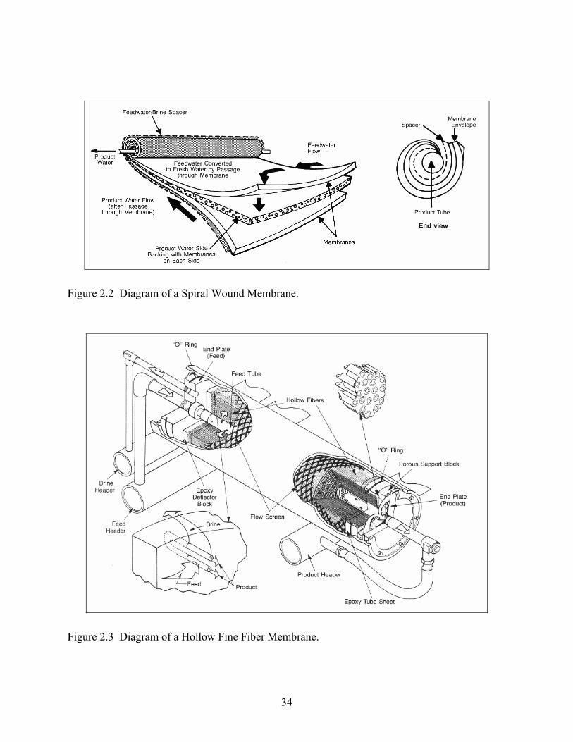
Figure 2.2 Diagram of a Spiral Wound Membrane.
Figure 2.3 Diagram of a Hollow Fine Fiber Membrane.
34

MASS TRANSPORT
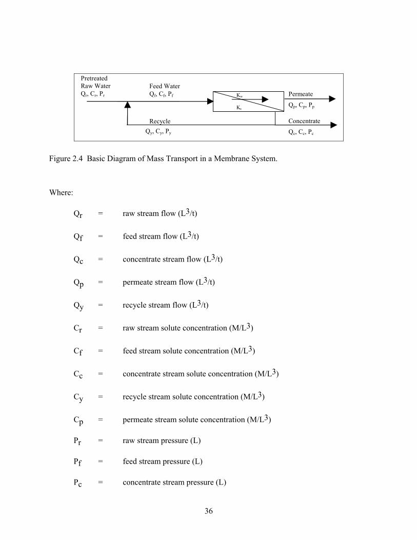
Figure 2.4 presents a basic diagram of mass transport in a membrane system. As shown,
a portion of feed water passes through the membrane material and exits the unit as permeate or
finished water. A portion of the feed water passes tangentially along the surface of the
membrane film and becomes more concentrated. This brine or concentrate stream is split with a
portion going to waste and a portion returned to the head of the system as a recycle flow. The
recycle flow is used to maintain a velocity across the surface of the membrane. Both solute and
solvent (water) pass through the membrane film as illustrated.
In an ideal membrane, solvent would readily pass through the membrane material while
solutes would be completely rejected. However, rejection of solutes it is only partially
successful; the solute mass transfer coefficient, Ks, represents the portion of solute that passes
through the membrane and is a rate term. The equivalent term for solvent passage is Kw, the
water mass transfer coefficient.
It is desirable to maximize the passage of water and minimize the passage of solute. This
would result in the lowest concentration of contaminants in the permeate or finished water
stream. Therefore membranes with higher Kw (passage of water) and lower Ks (passage of
solute) are preferred. However, as a membrane becomes fouled over time, the Kw declines
signifying a reduced water productivity.
35
Qy, Cy, Py
Recycle
Kw Ks
Pretreated Raw Water Qr, Cr, Pr
Feed Water Qf, Cf, Pf Permeate
Qp, Cp, Pp
Concentrate
Qc, Cc, Pc
Figure 2.4 Basic Diagram of Mass Transport in a Membrane System.
Where:
Qr = raw stream flow (L3/t)
Qf = feed stream flow (L3/t)
Qc = concentrate stream flow (L3/t)
Qp = permeate stream flow (L3/t)
Qy = recycle stream flow (L3/t)
Cr = raw stream solute concentration (M/L3)
Cf = feed stream solute concentration (M/L3)
Cc = concentrate stream solute concentration (M/L3)
Cy = recycle stream solute concentration (M/L3)
Cp = permeate stream solute concentration (M/L3)
Pr = raw stream pressure (L)
Pf = feed stream pressure (L)
Pc = concentrate stream pressure (L)
36
Py = recycle stream pressure (L)
Pp = permeate stream pressure (L)
Kw = solvent mass transfer coefficient (L2t/M)
Ks = solute mass transfer coefficient (L/t)
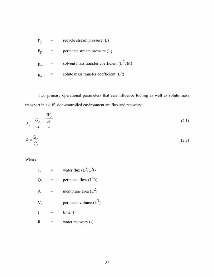
Two primary operational parameters that can influence fouling as well as solute mass
transport in a diffusion-controlled environment are flux and recovery:
At
V
AQ
J
p
pw
∂∂
== (2.1)
r
p
R = (2.2)
Where:
Jw = water flux (L3/L2t)
Qp = permeate flow (L3/t)
A = membrane area (L2)
Vp = permeate volume (L3)
t = time (t)
R = water recovery (-)
37

As shown, flux is the flow per unit area of membrane. Increases in flux represent
increased hydraulic loading and can lead to increased fouling. For solute mass transport
governed by diffusion, an increase in flux will result in a higher quality permeate due to the
increased passage of water occurring concurrent with a fixed passage of solute. Equation (2.2)
describes “recovery” or the fraction of water that passes through the membrane relative to the
total flow introduced. As recovery increases, the concentration of solute on the feed-side of the
membrane increases. Increasing recovery can also contribute to increased fouling as well as a
lesser quality permeate.
MASS TRANSPORT THEORIES
Mass transport equations have been developed for membrane systems to describe the
passage of components from the feed to permeate side of the membrane. Transport takes place
as a result of driving forces on the individual solutes in the feed. Transport equations for
membrane systems have primarily been physical models based on thermodynamics and/or
statistical mechanics (Bitter, 1991). These liquid separation theories can be placed in three main
categories:
• Irreversible thermodynamics;
• Preferential sorption-capillary flow theory; and
• Solution-diffusion theory
38

These theories were developed to explain the fundamentals of transport in clean
membranes and were not designed to address the effect of foulants. The most common theory
used in practice is the solution-diffusion theory, which describes solvent and solute flow by
Equations (2.3) and (2.4) respectively (Weber, 1972). According to the solution-diffusion
model, each permeant dissolves into the membrane material and passes by diffusion in response
to its chemical potential gradient. This theory assumes a semi permeable membrane surface
entirely controlled by diffusion with no porous areas capable of convective flow. However,
membrane surfaces can have imperfections, which allow a fraction of water through the film via
convective flow. Also, the solution-diffusion theory does not account for coupling effects such
as increased hardness rejection due to calcium-sulfate coupling. Never-the-less, experimental
mass transport results follow solution-diffusion theory and this theory is the most widely applied.
Equation (2.3) describes the solvent or water flux to be a function of the applied pressure
and the osmotic pressure due to the concentration gradient between the feed and permeate.
Equation (2.4) describes solute flux as function of the concentration gradient.
( )A
QPkJ p
Ww =∆Π−∆=
(2.3)
ACQ
CkJ ppss =∆= (2.4)
Where:
Jw = water flux (L3/L2t)
∆P = pressure gradient (L), [(Pf+Pc)/2-Pp]
∆Π = osmotic pressure (L) [(Πf+Πc)/2-Πp]
39

∆C = concentration gradient (M/L3),[(Cf+Cc)/2-Cp]
The solvent mass transfer coefficient, kw, or solvent permeability in Equation (2.3) was
developed from solution-diffusion theory to be a function of a number of factors as follows
(Weber, 1972):
RTlVCD
K wwwe = (2.5)
Where:
Dw = diffusivity of water in the membrane
Cw = concentration of water in the membrane
Vw = molar volume of water
R = gas constant
T = temperature
l = membrane thickness
The solvent mass transfer coefficient can be calculated from operational data and
manipulation of Equation (2.3):
( )∆Π−∆=
PJ
k wW (2.6)
The solvent mass transfer coefficient provides a productivity parameter normalized for
both flux and pressure. As shown in Equation (2.6), kw is proportional to flux and inversely
40

proportional to pressure. Additionally, kw is a function of temperature (Equation (2.5)) due to
the change in water viscosity with temperature. Therefore kw most be normalized for
temperature. Normalization for temperature can be calculated from Equation (2.5).
REFERENCES
Bitter, J. G., 1991. Transport Mechanisms in Membrane Separation Proceses, Plenum Press.
Gregor, H.P., 1976. Fixed-Charge Ultrafiltration Membranes, in Charge Gels and Membranes, Part 1, ed. E. Selegny, 57-69.
Hanemaaijer, J.H., Robbertsen, T., van den Boomgaard, Th., and Gunnick, J.W., 1989. Fouling of Ultrafiltration Membranes. The Role of Protein Adsorption and Salt Precipitation, Journal of Membrane Science, 40, 199-217.
Weber, W.J. Jr., 1972. Physicochemical Processes for Water Quality Control, John Wiley and Sons, New York, NY.
41
CHAPTER 3 EXPERIMENTAL METHODS AND PROCEDURES
The following Chapter presents a source water description, the methods and experimental
plans for the pilot-scale study and analytical methods. These represent methods common to all
experiments developed as part of this research. Specific methods associated with the research
presented in each of the peer-reviewed publications are provided within each of the papers
themselves, as presented later in this document.
RAW WATER SOURCE
The research conducted for this dissertation was part of a larger UCF project funded by
the United States Environmental Protection Agency. This larger project tested surface waters in
Bowling Green, Ohio and Tampa, Florida. This dissertation research was conducted at the
Tampa site, which utilizes raw water from the Hillsborough River. The Hillsborough River is a
spring-fed river with supplemental supply coming from precipitation and watershed runoff.
Water quality varies greatly between the wet and dry seasons. During the wet season (summer
months), storm water traveling through marsh areas brings highly organic fresh water to the river
and reduces hardness and alkalinity. Conversely, the dry season (winter months) is characterized
by lower organic levels and higher hardness and alkalinity. During the 15 months of operation, a
full range of quality was observed and is presented in Table 3.1 below. This data represents
biweekly sampling for the period from July 1997 through November 1999. As shown, the total
organic carbon (TOC) ranged from 4 to 28 mg/L, total hardness from 50 to 185 mg/L as CaCO3,
42

and alkalinity from 30 to 180 mg/L as CaCO3. Though typical of Florida surface waters, the
TOC levels of this river are higher than most other sources in the United States. This was
considered an advantage as it allowed assessment of integrated membrane systems under
challenging conditions, in terms of feed water organic content. In addition, the warm weather in
Florida and the abundance of organic material in the source water is conducive to biological
growth. Again this was desired as it represented challenging conditions for the use of membrane
systems, with respect to fouling potential and treatment requirements.
Table 3.1 Hillsborough River Raw Water Quality
Parameter Units Maximum Minimum Average
UV-254 (cm-1) 1.907 0.151 0.741
Color (cpu) 297 34 153
TOC (mg/L) 27.5 4.0 16.4
SDS chlorine dose (mg/L) 50.0 14.6 37.2
SDS chlorine residual (mg/L) 4.2 0.1 1.3
TOX (µg/L) 1540 508 922
SDI5 (units) >20 >20 >20
Particle Count (#/ml, >2.0 um) 62,608 1,446 13,235
Alkalinity (mg/L as CaCO3) 178 30 67
Total Hardness (mg/L as CaCO3) 184 50 108
TSS (mg/L) 15.1 1.6 4.7
TDS (mg/L) 270 63 169
TC (cfu/ml) 10,000 3 1,816
TON (units) 50.0 1.0 10.1
MIB (ng/L) 25.4 < 1.0 5.6
43
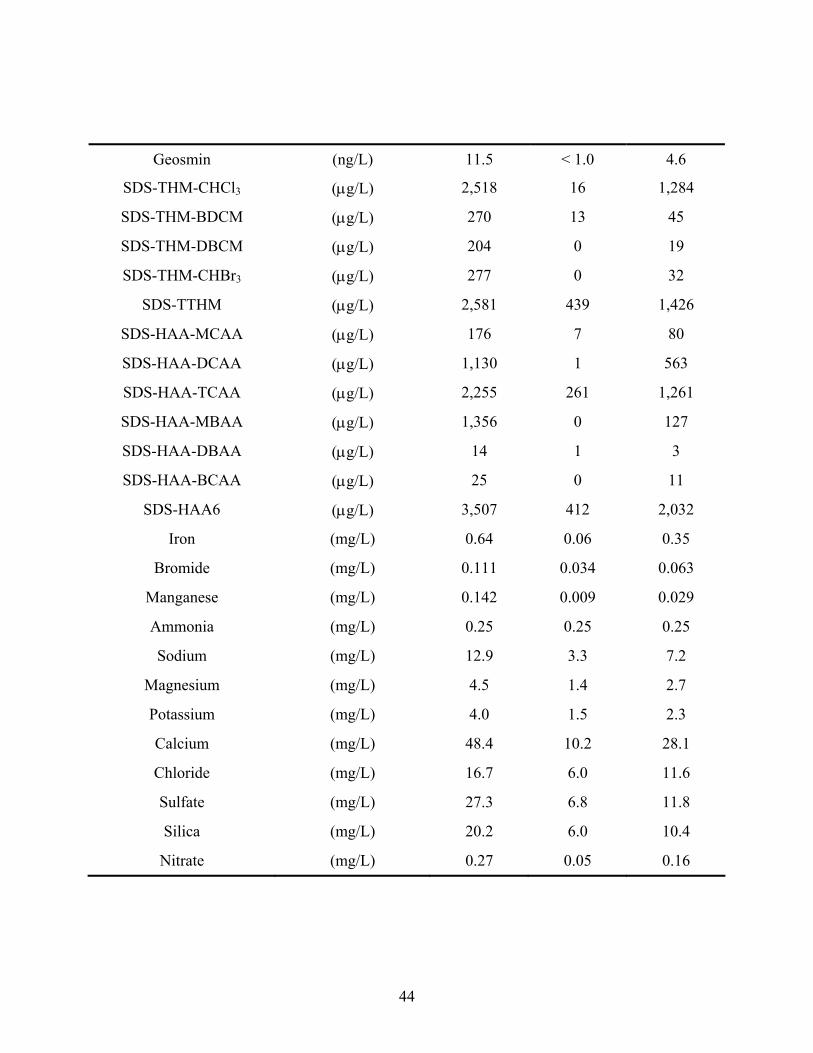
Geosmin (ng/L) 11.5 < 1.0 4.6
SDS-THM-CHCl3 (µg/L) 2,518 16 1,284
SDS-THM-BDCM (µg/L) 270 13 45
SDS-THM-DBCM (µg/L) 204 0 19
SDS-THM-CHBr3 (µg/L) 277 0 32
SDS-TTHM (µg/L) 2,581 439 1,426
SDS-HAA-MCAA (µg/L) 176 7 80
SDS-HAA-DCAA (µg/L) 1,130 1 563
SDS-HAA-TCAA (µg/L) 2,255 261 1,261
SDS-HAA-MBAA (µg/L) 1,356 0 127
SDS-HAA-DBAA (µg/L) 14 1 3
SDS-HAA-BCAA (µg/L) 25 0 11
SDS-HAA6 (µg/L) 3,507 412 2,032
Iron (mg/L) 0.64 0.06 0.35
Bromide (mg/L) 0.111 0.034 0.063
Manganese (mg/L) 0.142 0.009 0.029
Ammonia (mg/L) 0.25 0.25 0.25
Sodium (mg/L) 12.9 3.3 7.2
Magnesium (mg/L) 4.5 1.4 2.7
Potassium (mg/L) 4.0 1.5 2.3
Calcium (mg/L) 48.4 10.2 28.1
Chloride (mg/L) 16.7 6.0 11.6
Sulfate (mg/L) 27.3 6.8 11.8
Silica (mg/L) 20.2 6.0 10.4
Nitrate (mg/L) 0.27 0.05 0.16
44

PILOT STUDY
Following site selection and a nanofiltration membrane selection study, the pilot study
experimental plan was developed. Given that the source water for the project was an organic
surface water, pretreatment processes were identified to extend nanofiltration operational time,
between chemical cleanings. The pretreatment processes would be fed Hillsborough River water
obtained from the Tampa Water Department’s reservoir. The pretreated water would then be fed
to a nanofiltration treatment unit. The pretreatment processes would be capable of removing
microorganisms and turbidity as well as pretreat the raw water prior to NF treatment. The NF
membranes would be used to remove DBP precursors and TDS, among other constituents. Four
types of pretreatment processes were proposed for evaluation.
• Ferric chloride coagulation, settling, and sand filtration (CSF);
• Microfiltration (MF);
• Ultrafiltration (UF); and
• In-line coagulation of microfiltration units (C/MF).
Pilot Treatment Trains
As part of the pilot study, the following treatment processes were evaluated:
• Three low pressure pretreatment membranes:
MMF - the Memcor 0.2 µm pore size microfilter;
UF - the Aquasource 0.01 µm pore size ultrafilter; and
45

ZMF – the Zenon 0.2 µm pore size microfilter.
• In-line coagulation of the above three pretreatment units.
• Conventional coagulation, sedimentation, and filtration (CSF) pretreatment.
• Three nanofiltration membranes
Hydranautics ESNA CTF membrane;
Hydranautics LFC1 CTF membrane; and
Fluid Systems CALP CA membrane.
These unit processes were integrated to form process trains as presented in Figure 3.1.
RawWater
Coagulation/Sedimentation/
Dechlorination Nanofiltration
Permeate
Concentrate
CSF-NF
C-MF-NF
MF/UF-NF
RawWater
Ultrafiltration/Microfiltration
Nanofiltration
Permeate
Concentrate
Backwash
RawWater
In-lineCoagulation
Microfiltration Nanofiltration
Permeate
Concentrate
Backwash
Sand Filtration
Figure 3.1 Treatment Process Trains
46

NF Operational Conditions
Nanofiltration systems were operated using various pretreatment processes listed above
and discussed in detail following this section. For each integrated membrane system, a set of
four NF experiments were conducted as shown in Table 3.2. These experiments consisted of
varying flux and recovery. For all experiments, the feed water from the pretreatment unit
underwent conventional membrane pretreatment consisting of acidification and/or antiscalent
addition followed by 5 µm static microfiltration. Operational conditions for each pretreatment
system are described in the following sections.
Table 3.2 NF Operational Conditions
Flux Recovery (gfd) (percent) Experiment
7 14 65 85 1 X X 2 X X 3 X X 4 X X
CSF-NF Pilot Testing
For the coagulation/sedimentation/filtration-nanofiltration (CSF-NF) system, CSF water
was obtained from the full-scale water treatment plant. Due to prechlorination at the full-scale
plant, the CSF water contains a free chlorine residual, which the nanofilters are not able to
tolerate. This residual was removed by processing the CSF water through a granular activated
carbon filter (7.0 sf surface area) that had been exhausted of TOC removal capacity but was
capable of fully removing the chlorine residual. Coagulation/sedimentation conditions (chemical
47

doses, loading rates, etc.) were a function of the needs of the full-scale WTP and were not
controllable for this pilot study. However, conditions were monitored and recorded. During the
course of testing, ferric sulfate was dosed at an average of 170 mg/L (2.6 meq/L).
UF-NF Pilot Testing
Ultrafiltration is shown in Figure 3.1 to be a membrane process with a pore size one to
two orders of magnitude larger than nanofiltration. Ultrafiltration requires relatively low
pressures of 40 psi or less and is effective for removal of particulate matter such as organic
particles, bacteria, and viruses. An Aquasource brand ultrafiltration unit was used in this
research but was not of adequate size to provide sufficient filtrate flow to feed UCF’s 2-1 array
NF system. The UF unit was capable of providing feed water to a single element NF system.
Therefore the seventh pressure vessel in the UCF trailer was utilized as a single element NF
system using Aquasource UF filtrate as feed water. The Aquasource unit consists of hollow fiber
cellulose acetate membranes with a pore size of 0.01 microns. This process requires no chemical
addition. Experiments were conducted as shown in Table 3.3 to determine optimum UF
conditions.
Note, the Aquasource UF system data is only presented in the Appendix of this
dissertation due to its lack of sustainable and acceptable performance for this research. No
performance information or results for the Aquasource UF membrane are provided in the body of
this document.
48
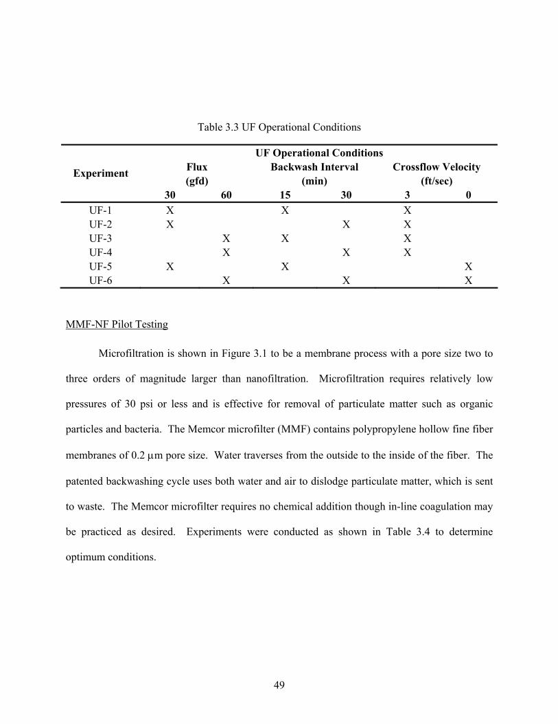
Table 3.3 UF Operational Conditions
UF Operational Conditions Flux Backwash Interval Crossflow Velocity (gfd) (min) (ft/sec)
Experiment
30 60 15 30 3 0 UF-1 X X X UF-2 X X X UF-3 X X X UF-4 X X X UF-5 X X X UF-6 X X X
MMF-NF Pilot Testing
Microfiltration is shown in Figure 3.1 to be a membrane process with a pore size two to
three orders of magnitude larger than nanofiltration. Microfiltration requires relatively low
pressures of 30 psi or less and is effective for removal of particulate matter such as organic
particles and bacteria. The Memcor microfilter (MMF) contains polypropylene hollow fine fiber
membranes of 0.2 µm pore size. Water traverses from the outside to the inside of the fiber. The
patented backwashing cycle uses both water and air to dislodge particulate matter, which is sent
to waste. The Memcor microfilter requires no chemical addition though in-line coagulation may
be practiced as desired. Experiments were conducted as shown in Table 3.4 to determine
optimum conditions.
49
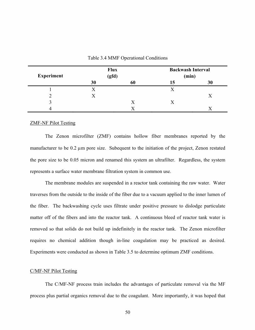
Table 3.4 MMF Operational Conditions
Flux Backwash Interval (gfd) (min) Experiment
30 60 15 30 1 X X 2 X X 3 X X 4 X X
ZMF-NF Pilot Testing
The Zenon microfilter (ZMF) contains hollow fiber membranes reported by the
manufacturer to be 0.2 µm pore size. Subequent to the initiation of the project, Zenon restated
the pore size to be 0.05 micron and renamed this system an ultrafilter. Regardless, the system
represents a surface water membrane filtration system in common use.
The membrane modules are suspended in a reactor tank containing the raw water. Water
traverses from the outside to the inside of the fiber due to a vacuum applied to the inner lumen of
the fiber. The backwashing cycle uses filtrate under positive pressure to dislodge particulate
matter off of the fibers and into the reactor tank. A continuous bleed of reactor tank water is
removed so that solids do not build up indefinitely in the reactor tank. The Zenon microfilter
requires no chemical addition though in-line coagulation may be practiced as desired.
Experiments were conducted as shown in Table 3.5 to determine optimum ZMF conditions.
C/MF-NF Pilot Testing
The C/MF-NF process train includes the advantages of particulate removal via the MF
process plus partial organics removal due to the coagulant. More importantly, it was hoped that
50
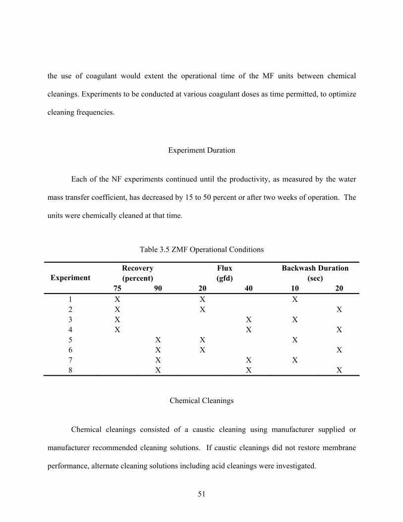
the use of coagulant would extent the operational time of the MF units between chemical
cleanings. Experiments to be conducted at various coagulant doses as time permitted, to optimize
cleaning frequencies.
Experiment Duration
Each of the NF experiments continued until the productivity, as measured by the water
mass transfer coefficient, has decreased by 15 to 50 percent or after two weeks of operation. The
units were chemically cleaned at that time.
Table 3.5 ZMF Operational Conditions
Recovery Flux Backwash Duration (percent) (gfd) (sec) Experiment
75 90 20 40 10 20 1 X X X 2 X X X 3 X X X 4 X X X 5 X X X 6 X X X 7 X X X 8 X X X
Chemical Cleanings
Chemical cleanings consisted of a caustic cleaning using manufacturer supplied or
manufacturer recommended cleaning solutions. If caustic cleanings did not restore membrane
performance, alternate cleaning solutions including acid cleanings were investigated.
51

Sampling and Data Collection
Sampling locations are identified in Figure 3.2. Water quality samples were collected
according to the schedule in Table 3.6. Flow and pressure data were collected three times per
day. Table 3.7 presents the operational data collection schedule.
Permeate
ConcentrateStage 1 Stage 2Acid/AAaddition
NanofiltrationTrain 1
11 12 16
15
14
13 17
Recycle18
Permeate
ConcentrateStage 1 Stage 2Acid/AAaddition
NanofiltrationTrain 2
21 22 26
25
24
23 27
Recycle
28
Permeate
Concentrate Stage 1 Acid/AAaddition
NanofiltrationTrain 3
31 32 36
37
Recycle
38
1
Memcor MF Pretreatment
3
CSF Pretreatment
5
Aquasource UF Pretreatment
4
2 Zenon MF Pretreatment
Figure 3.2 Sampling/Gauge Location Diagram.
52
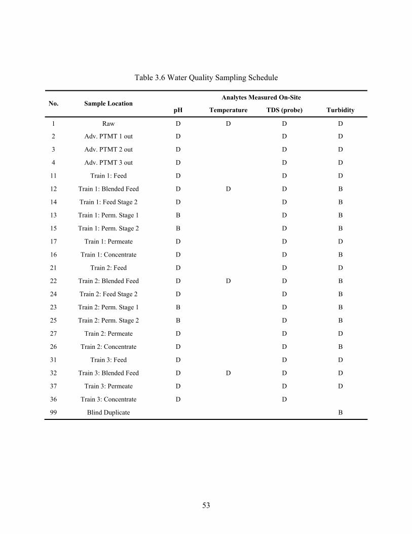
Table 3.6 Water Quality Sampling Schedule
Analytes Measured On-Site No. Sample Location
pH Temperature TDS (probe) Turbidity
1 Raw D D D D
2 Adv. PTMT 1 out D D D
3 Adv. PTMT 2 out D D D
4 Adv. PTMT 3 out D D D
11 Train 1: Feed D D D
12 Train 1: Blended Feed D D D B
14 Train 1: Feed Stage 2 D D B
13 Train 1: Perm. Stage 1 B D B
15 Train 1: Perm. Stage 2 B D B
17 Train 1: Permeate D D D
16 Train 1: Concentrate D D B
21 Train 2: Feed D D D
22 Train 2: Blended Feed D D D B
24 Train 2: Feed Stage 2 D D B
23 Train 2: Perm. Stage 1 B D B
25 Train 2: Perm. Stage 2 B D B
27 Train 2: Permeate D D D
26 Train 2: Concentrate D D B
31 Train 3: Feed D D D
32 Train 3: Blended Feed D D D D
37 Train 3: Permeate D D D
36 Train 3: Concentrate D D
99 Blind Duplicate B
53
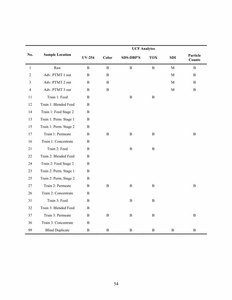
UCF Analytes
No. Sample Location UV-254 Color SDS-DBP'S TOX SDI Particle
Counts
1 Raw B B B B M B
2 Adv. PTMT 1 out B B M B
3 Adv. PTMT 2 out B B M B
4 Adv. PTMT 3 out B B M B
11 Train 1: Feed B B B
12 Train 1: Blended Feed B
14 Train 1: Feed Stage 2 B
13 Train 1: Perm. Stage 1 B
15 Train 1: Perm. Stage 2 B
17 Train 1: Permeate B B B B B
16 Train 1: Concentrate B
21 Train 2: Feed B B B
22 Train 2: Blended Feed B
24 Train 2: Feed Stage 2 B
23 Train 2: Perm. Stage 1 B
25 Train 2: Perm. Stage 2 B
27 Train 2: Permeate B B B B B
26 Train 2: Concentrate B
31 Train 3: Feed B B B
32 Train 3: Blended Feed B
37 Train 3: Permeate B B B B B
36 Train 3: Concentrate B
99 Blind Duplicate B B B B B B
54

TWD Analytes
No. Sample Location Alkalinityand Total Hardness
TOC TSS TDS TC,
TON, Spores
MIB and
geosmin
THM and
HAA Iron Bromide
1 Raw B B B B B B B B B
2 Adv. PTMT 1 out B B B B B B B
3 Adv. PTMT 2 out B B B B B B B
4 Adv. PTMT 3 out B B B B B B B
11 Train 1: Feed B B B B B B
12 Train 1: Blended Feed B B B
14 Train 1: Feed Stage 2 B B B
13 Train 1: Perm. Stage 1 B B B
15 Train 1: Perm. Stage 2 B B B
17 Train 1: Permeate B B B B B B B B
16 Train 1: Concentrate B B B B
21 Train 2: Feed B B B B B B
22 Train 2: Blended Feed B B B
24 Train 2: Feed Stage 2 B B B
23 Train 2: Perm. Stage 1 B B B
25 Train 2: Perm. Stage 2 B B B
27 Train 2: Permeate B B B B B B B B
26 Train 2: Concentrate B B B B
31 Train 3: Feed B B B B B B
32 Train 3: Blended Feed B B B
37 Train 3: Permeate B B B B B B B B
36 Train 3: Concentrate B B B B
99 Blind Duplicate B B B B B B B B B
55

TWD Analytes
No. Sample Location Manganese Ammonia Sodium Chloride Sulfate Silica Nitrate
1 Raw B B B B B B B
2 Adv. PTMT 1 out B B B B B B B
3 Adv. PTMT 2 out B B B B B B B
4 Adv. PTMT 3 out B B B B B B B
11 Train 1: Feed B B B B B
12 Train 1: Blended Feed
14 Train 1: Feed Stage 2
13 Train 1: Perm. Stage 1
15 Train 1: Perm. Stage 2
17 Train 1: Permeate B B B B B B B
16 Train 1: Concentrate B B
21 Train 2: Feed B B B B
22 Train 2: Blended Feed B
24 Train 2: Feed Stage 2
23 Train 2: Perm. Stage 1
25 Train 2: Perm. Stage 2
27 Train 2: Permeate B B B B B B B
26 Train 2: Concentrate B B
31 Train 3: Feed B B B B B
32 Train 3: Blended Feed B
37 Train 3: Permeate B B B B B B B
36 Train 3: Concentrate B
99 Blind Duplicate B B B B B B B
D – daily B - biweekly
56

Table 3.7 Operational Data Collection Schedule
Location Frequency1
Pretreatment Units Flow in 3/day Flow out 3/day Pressure in 3/day Pressure out 3/day
NF units Feed flow 3/day Feed pressure 3/day Blended feed flow 3/day Blended feed pressure 3/day Permeate flow 3/day Permeate pressure 3/day Total concentrate flow 3/day Total concentrate pressure 3/day Concentrate-to-waste flow 3/day
ANALYTICAL METHODS
Water quality analyses were performed by the Civil and Environmental Engineering
Department Laboratory and by the Tampa Water Department Laboratory Services. All
analytical work was carried out in accordance with published standard methods, where such
methods exist. Table 3.8 lists the parameters for which a standard method was available.
Following this table are the procedures used for the remaining parameters evaluated in this
research.
57
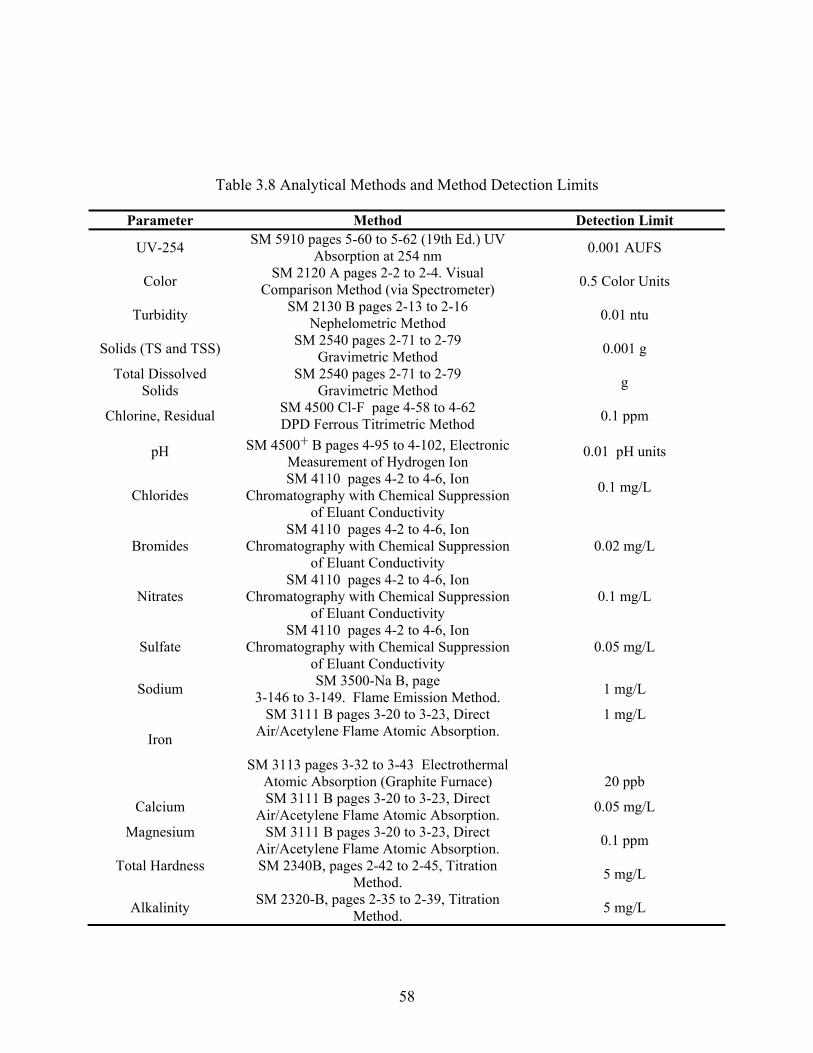
Table 3.8 Analytical Methods and Method Detection Limits
Parameter Method Detection Limit
UV-254 SM 5910 pages 5-60 to 5-62 (19th Ed.) UV Absorption at 254 nm 0.001 AUFS
Color SM 2120 A pages 2-2 to 2-4. Visual Comparison Method (via Spectrometer) 0.5 Color Units
Turbidity SM 2130 B pages 2-13 to 2-16 Nephelometric Method 0.01 ntu
Solids (TS and TSS) SM 2540 pages 2-71 to 2-79 Gravimetric Method 0.001 g
Total Dissolved Solids
SM 2540 pages 2-71 to 2-79 Gravimetric Method g
Chlorine, Residual SM 4500 Cl-F page 4-58 to 4-62 DPD Ferrous Titrimetric Method 0.1 ppm
pH SM 4500+ B pages 4-95 to 4-102, Electronic Measurement of Hydrogen Ion
0.01 pH units
Chlorides SM 4110 pages 4-2 to 4-6, Ion
Chromatography with Chemical Suppression of Eluant Conductivity
0.1 mg/L
Bromides SM 4110 pages 4-2 to 4-6, Ion
Chromatography with Chemical Suppression of Eluant Conductivity
0.02 mg/L
Nitrates SM 4110 pages 4-2 to 4-6, Ion
Chromatography with Chemical Suppression of Eluant Conductivity
0.1 mg/L
Sulfate SM 4110 pages 4-2 to 4-6, Ion
Chromatography with Chemical Suppression of Eluant Conductivity
0.05 mg/L
Sodium SM 3500-Na B, page 3-146 to 3-149. Flame Emission Method. 1 mg/L
Iron
SM 3111 B pages 3-20 to 3-23, Direct Air/Acetylene Flame Atomic Absorption.
SM 3113 pages 3-32 to 3-43 Electrothermal
Atomic Absorption (Graphite Furnace)
1 mg/L
20 ppb
Calcium SM 3111 B pages 3-20 to 3-23, Direct Air/Acetylene Flame Atomic Absorption. 0.05 mg/L
Magnesium
SM 3111 B pages 3-20 to 3-23, Direct Air/Acetylene Flame Atomic Absorption. 0.1 ppm
Total Hardness
SM 2340B, pages 2-42 to 2-45, Titration Method. 5 mg/L
Alkalinity SM 2320-B, pages 2-35 to 2-39, Titration Method. 5 mg/L
58
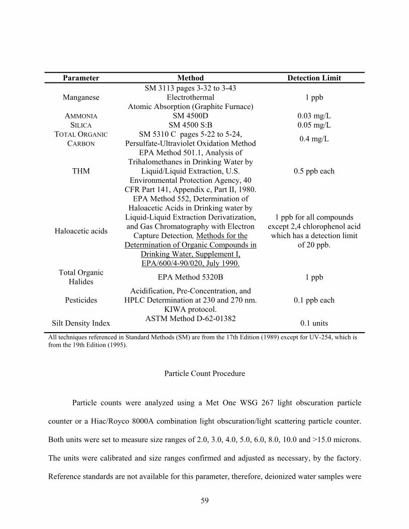
Parameter Method Detection Limit
Manganese SM 3113 pages 3-32 to 3-43
Electrothermal Atomic Absorption (Graphite Furnace)
1 ppb
AMMONIA SM 4500D 0.03 mg/L SILICA SM 4500 S:B 0.05 mg/L
TOTAL ORGANIC CARBON
SM 5310 C pages 5-22 to 5-24, Persulfate-Ultraviolet Oxidation Method 0.4 mg/L
THM
EPA Method 501.1, Analysis of Trihalomethanes in Drinking Water by
Liquid/Liquid Extraction, U.S. Environmental Protection Agency, 40
CFR Part 141, Appendix c, Part II, 1980.
0.5 ppb each
Haloacetic acids
EPA Method 552, Determination of Haloacetic Acids in Drinking water by
Liquid-Liquid Extraction Derivatization, and Gas Chromatography with Electron
Capture Detection, Methods for the Determination of Organic Compounds in
Drinking Water, Supplement I, EPA/600/4-90/020, July 1990.
1 ppb for all compounds except 2,4 chlorophenol acid which has a detection limit
of 20 ppb.
Total Organic Halides EPA Method 5320B 1 ppb
Pesticides Acidification, Pre-Concentration, and
HPLC Determination at 230 and 270 nm. KIWA protocol.
0.1 ppb each
Silt Density Index ASTM Method D-62-01382 0.1 units
All techniques referenced in Standard Methods (SM) are from the 17th Edition (1989) except for UV-254, which is from the 19th Edition (1995).
Particle Count Procedure
Particle counts were analyzed using a Met One WSG 267 light obscuration particle
counter or a Hiac/Royco 8000A combination light obscuration/light scattering particle counter.
Both units were set to measure size ranges of 2.0, 3.0, 4.0, 5.0, 6.0, 8.0, 10.0 and >15.0 microns.
The units were calibrated and size ranges confirmed and adjusted as necessary, by the factory.
Reference standards are not available for this parameter, therefore, deionized water samples were
59
tested to confirm background particle count levels and ensure the units were performing
consistently. Deionized water contained no more than 75 particles per ml. If values higher than
this were obtained, the unit was either flushed with ethyl alcohol or the sensor walls were
cleaned with unwaxed dental floss, in accordance with the manufacturers instructions.
Following cleaning and baseline stabilization, samples were analyzed in duplicate. Samples
requiring dilution were adjusted not only for the dilution factor but also for the baseline level of
particles present in the deionized water.
60
CHAPTER 4 SURFACE WATER TREATMENT USING NANOFILTRATION – PILOT TESTING RESULTS AND DESIGN
CONSIDERATIONS
INTRODUCTION
Nanofiltration (NF) and reverse osmosis (RO) processes have a history of providing a
water quality superior to that obtained from conventional treatment technologies. The organic
and inorganic removal capabilities of NF/RO are well known for treatment of seawater and
groundwater. Extending their application to surface waters is logical and desirable, given
increasingly stringent regulations and quality concerns with many surface waters. However,
spiral wound NF/RO systems foul rapidly when treating surface water (Reiss et al., 1996; Reiss
and Taylor, 1991). One potential solution is the use of an advanced pretreatment process prior to
NF/RO treatment. Such treatment systems, operated in series, are designated Integrated
Membrane Systems (IMSs).
This research focuses on the factors affecting successful multi-stage pilot-scale operation
of IMSs to treat a highly organic surface water. Fifteen months of pilot-scale nanofiltration of
the Hillsborough River in Tampa, Florida, US have yielded important operational and design
considerations. This paper presents water quality and fouling results for various IMS process
trains. In addition, fouling mechanisms are explored and critical design criteria for sustained
operation are presented.
61
SOURCE WATER
The source water was the Hillsborough River in eastern Hillsborough County, Florida.
The Tampa Water Department owns and operates an 80 mgd conventional ferric coagulation,
sedimentation, filtration (CSF) water treatment plant (WTP), subsequently expanded to 120 mgd,
that was the site for this pilot study. The Hillsborough River is a spring-fed river with
supplemental supply coming from precipitation and watershed runoff. Water quality varies
greatly between seasons with higher organic levels and lower TDS during the wet (summer)
season and higher TDS and lower organic levels during the dry (winter) season.
Water quality observed during 15 months of operation is presented in Table 4.1. As
shown, the total organic carbon (TOC) ranged from 4 to 28 mg/L, total hardness from 50 to 160
mg/L as CaCO3, and alkalinity from 30 to 180 mg/L as CaCO3. Though typical of Florida
surface waters, the TOC levels of this river are higher than most other sources in the United
States.
PILOT STUDY
IMSs were developed to address four fouling mechanisms of concern:
• Precipitation;
• Plugging;
• Organic adsorption; and
• Biofouling.
62

Applicable pretreatment methods are shown in Table 4.2 and were evaluated for use prior
to nanofiltration. Acid and antiscalent addition was chosen for control of precipitation as is
necessary for all nanofiltration systems. Two microfilters were selected for turbidity reduction,
the Memcor MF (MMF) and Zenon MF (ZMF). Additionally, these MF units were evaluated
with in-line coagulation (C/MMF and C/ZMF) for reduction of organic levels. Monochloramine
was used during a portion of the study, for control of attached bacterial growth. Finally, three
nanofilters were evaluated. Microfiltration (MF) and NF specifications are presented in Table
4.3.
Table 4.1 Hillsborough River Raw Water Quality
Parameter Units Maximum Minimum Average
TOC (mg/L) 27.5 4.0 16.4
SDS-TTHM (µg/L) 2,581 199 1,224
SDS-HAA6 (µg/L) 3,507 254 1,683
Alkalinity (mg/L as CaCO3) 178 30 80
Total Hardness (mg/L as CaCO3) 184 50 108
TDS (mg/L) 270 63 169
MIB (ng/L) 25.4 < 1.0 7.4
Geosmin (ng/L) 11.5 < 1.0 4.6
63

Table 4.2 Pretreatment Methods by Fouling Mechanism
Organic Adsoprtion Advanced Pretreatment Precipitation Plugging Biofouling
Acid/Antiscalent √ CSF √ √
MF √ C/MF √ √
Biocide √ CSF: coagulation, sedimentation, filtration MF: microfiltration C/MF: In-line coagulation, microfiltration
Table 4.3 Membrane Characteristics
Nominal Pore Size MWCO Membrane Configuration
(µm) (daltons)Material
No. of modules/ elements
Array
Memcor microfilter hollow fiber 0.2 na polypropylene 3 1
Zenon microfilter hollow fiber 0.1 na proprietary 3 1
Fluid Systems CALP
nanofilter spiral wound na 300
cellulose acetate
derivative 6 2-1
Hydranautics ESNA
nanofilter spiral wound na 250 polyamide
composite 9 2-1
Hydranautics LFC1
nanofilter spiral wound na 200 polyamide
composite 9 2-1
These unit processes were developed as process trains and tested as shown in Figure 4.1.
An operational matrix of four - two week experiments for each process train was developed.
Fluxes of 7 and 14 gfd (12 and 23 L/hr/m2)and recoveries of 65 and 85 percent were specified for
a total of four experiments totaling 8 weeks of operation, for each pretreatment process.
64
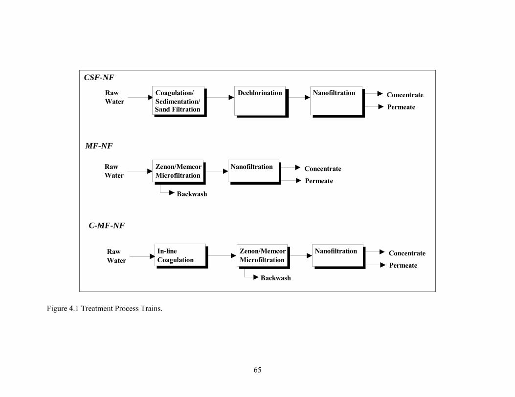
RawWater
Coagulation/Sedimentation/
Dechlorination Nanofiltration
Permeate
Concentrate
CSF-NF
C-MF-NF
MF-NF
RawWater
Zenon/MemcorMicrofiltration
Nanofiltration
Permeate
Concentrate
Backwash
RawWater
In-lineCoagulation
Zenon/MemcorMicrofiltration
Nanofiltration
Permeate
Concentrate
Backwash
Sand Filtration
Figure 4.1 Treatment Process Trains.
65

The Zenon (ZMF) and Memcor (MMF) unit processes consisted of pilot-scale units
installed at the WTP site. The ZMF unit is capable of producing 5 to 12 gpm (19 to 45 L/min) of
filtrate. The MMF unit produces 8 to 30 gpm (30 to 114 L/min) of filtrate. The CSF pretreated
water was obtained from the full-scale WTP. This surface water treatment plant employs ferric
sulfate coagulation, sedimentation, and sand filtration. The raw water was dosed with ferric
sulfate at an average of 170 mg/L (2.6 meq/L) during the 15 month testing period. The WTP
employs prechlorination therefore a residual of free chlorine is present in the filtrate. This can
damage the nanofilters therefore was removed via granular activated carbon (GAC) filtration.
The 7.0 sf (0.7 m2) surface area filter had been exhausted of TOC removal capacity, to prevent
further organic matter removal by GAC, but chlorine removal was complete during the entire
testing period.
Filtrate from the ZMF, MMF, and CSF processes was pumped to the nanofiltration units
where hydrochloric acid and/or Argo Scientific Hypersperse 200 antiscalent were added. The
hydrochloric acid was added at a dose sufficient to prohibit calcium carbonate scaling and
minimize nanofilter hydrolysis. A target pH of 5.5 was maintained. Hypersperse 200 is
designed to prohibit iron fouling and was dosed at 2.5 mg/L for 85 percent NF recovery and 5.0
mg/L for 65 percent NF recovery. The nanofiltration pilot-plants are 2-1 array systems with
three 4-inch diameter by 40-inch long (0.1 m by 1 m) elements per pressure vessel. The CALP
nanofilter is a cellulose acetate (CA) derivative therefore is susceptible to biodegradation and/or
hydrolysis. The ESNA and LFC1 nanofilters are polyamide composite thin film membranes and
are not susceptible to biological degradation or hydrolysis.
66

PRODUCTIVITY RESULTS
Productivity was measured by the water mass transfer coefficient, which accounts for
changes in both flux and pressure via Equation (4.1) below:
( )KJ
PWW=−∆ ∆π
(4.1)
Where:
Jw = water flux (gfd, L/hr/m2)
∆P = pressure gradient (psi, bar)
∆π = osmotic pressure (psi, bar)
Kw = water mass transfer coefficient (gfd/psi, L/hr/m2/bar)
Process Design Issues
Primary issues for IMS treatment of surface water that evolved from the 15 months of
pilot-scale testing were:
• Biodegradation (associated with CALP);
• Irreversible fouling (associated with ESNA); and
• Biofouling and oxidative degradation (associated with LFC1).
67

Over the course of testing, each of these issues was addressed and corrective measures
implemented, where possible. These issues and the productivity results for the three nanofilters
are discussed in this section.
CALP
Initial tests of the CALP nanofilter used CSF pretreated water and antiscalent addition.
During operation with CSF feed water, no fouling was observed and productivity was consistent,
indicating the CALP membrane was not affected by precipitation, biogrowth, organic adsorption,
or particulate fouling. Following two months of operation, the CSF feed was replaced by ZMF
feed. The ZMF pretreatment reduced turbidity to less than 0.15 NTU but removed no dissolved
organic carbon (DOC). At 7 days of operation using ZMF feed water, the Kw of the CALP
increased dramatically and TDS rejection fell to zero, indicating no treatment of the feed water
and complete loss of membrane integrity.
Suspecting either biodegradation or hydrolysis, tests were performed using a single
element CALP system with and without acid and monochloramine addition. Heterotrophic plate
counts (HPCs) were monitored for characterization of bioactivity. Productivity results are shown
in Figure 4.2. Integrity was lost during the fourth experiment, which used no monochloramine or
acid addition. In addition, HPC concentrations at the end of this experiment were 103 colony
forming units per milliliter (cfu/ml) in the feed compared to 105 cfu/ml and 105.7 cfu/ml in the
permeate and concentrate, respectively. This showed biodegradation to be the cause of failure as
opposed to hydrolysis of the membrane. The success of the pH-adjusted experiment is attributed
68
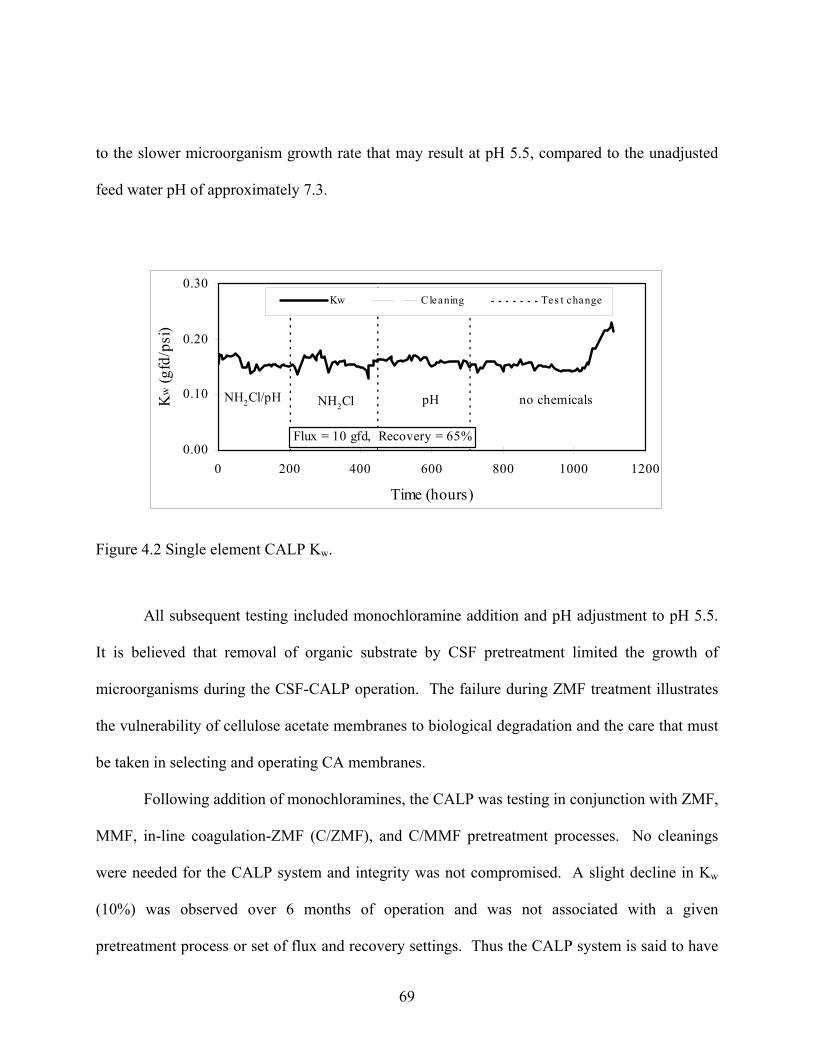
to the slower microorganism growth rate that may result at pH 5.5, compared to the unadjusted
feed water pH of approximately 7.3.
0.00
0.10
0 200 400 600 800 1000 1200
Time (hours)
w (g
0.20
0.30
Kfd
/psi
)
Kw Cleaning Tes t change
Flux = 10 gfd, Recovery = 65%
NH2Cl/pH NH Cl pH no chemicals
Figure 4.2 Single element CALP K .
pretreatment processes. No cleanings
were needed for the CALP system and integrity was not compromised. A slight decline in Kw
(10%) was observed over 6 months of operation and was not associated with a given
pretreatment process or set of flux and recovery settings. Thus the CALP system is said to have
2
w
All subsequent testing included monochloramine addition and pH adjustment to pH 5.5.
It is believed that removal of organic substrate by CSF pretreatment limited the growth of
microorganisms during the CSF-CALP operation. The failure during ZMF treatment illustrates
the vulnerability of cellulose acetate membranes to biological degradation and the care that must
be taken in selecting and operating CA membranes.
Following addition of monochloramines, the CALP was testing in conjunction with ZMF,
MMF, in-line coagulation-ZMF (C/ZMF), and C/MMF
69
a 9-month cleaning frequency, based on a criterion of 15% decline in Kw. The virtual absence of
fouling
ESNA
using the CALP membrane is significant and shows this film is not susceptible to organic
adsorption at TOC levels greater than 20 mg/L.
ere controlled. Though biocides or
oxygen-scavenging chemicals could be applied to this system to eliminate the potential for
th, the inability to clean this membrane, once fouled, was considered sufficient to
elimina
LFC1
Testing of the 2-1 array ESNA system was initiated using CSF pretreated feed water. No
biocide was used. Acid was not added; the feed water averaged pH 6.6. A 40% decline in Kw
was observed over 1,600 hours of operation. Chemical cleanings using both acidic and basic
cleaning solutions were performed at 515 hours and 1,600 hours of operation but did not recover
the productivity. Factory cleaning of a single element shipped back to the manufacturer also
resulted in marginal improvements in performance. Based on an extensive cleaning
investigation, it was concluded that the ESNA membrane was irreversibly fouled. No HPC data
were obtained during operation therefore it is not known if the fouling was due to adsorption or
biogrowth. However, precipitation and particulate loading w
biogrow
te it from further consideration at this site. A replacement nanofilter, the LFC1, was
proposed by Hydranautics and tested in lieu of the ESNA.
MMF feed. A bioinhibitor was not used for the first 1,000 hours of operation. Productivity
The LFC1 was presented as a less-negatively charged, low fouling, polyamide
membrane. The 2-1 array LFC1 system was initiated with acid and antiscalent addition and
70
results are shown in Figure 4.3. The LFC1 fouled under these conditions; however, chemical
cleanings were able to restore performance. Following discussions with Hydranautics, it was
determined that the LFC1 is monochloramine-tolerant. A monochloramine addition system was
installed and the NF system tested with CSF and MF pretreatment processes, beginning at 1,000
hours o
ime as TDS rejection (as measured by
probe)
ld result in favorable operation using this membrane. However, the
LFC1, based on this testing, is not monochloramine tolerant. Barring the development of an
alternate, National Sanitary Foundation-approved biocide, the LFC1 membrane is not a viable
choice for use at this site.
f operation. As shown, LFC1 performance was greatly improved with monochloramine
addition. Some fouling was observed in individual experiments however, the overall
performance was improved.
More importantly, the Kw increased over time, starting at 1,100 hours of operation. This
corresponds to the inception of monochloramine addition. To confirm the suspected degradation
of the film due to oxidation, TDS rejection was calculated and plotted over time (Figure 4.3). As
shown, there was partial loss of membrane integrity over t
started at 100% and decreased to 90% at the end of testing. It was concluded that the
LFC1 suffered from chemical oxidation due to monochloramine addition. This damage resulted
in an increase in Kw and a decrease in rejection over time.
In summary, biofouling was a significant fouling mechanism for the LFC1 membrane.
Control of biofouling cou
71

0.00
0.05
0.10
0.15
0.20
0.25
0.30
0.35
0.40
0 1000 2000 3000 4000 5000Time (hours)
Kw (g
fd/p
si)
50
60
70
80
90
100
110
Rej
ectio
n (%
)
Stage 1 Kw Stage 2 Kw CleaningTest Change S1 TDS Rejection S2 TDS Rejection
MMF ZMFCSFZMF C/MMF MMF
Figure 4.3 LFC1 Kw and TDS rejection.
Surface Characterization
The order of membrane fouling for this study was ESNA>LFC1>CALP. To determine
the cause for such differences, a surface characterization study was conducted to quantify
relative charge and roughness. All membrane systems had been operated for control of particle
fouling and precipitation. Additionally, biological fouling was controlled during certain periods
of operation with the CALP and LFC1. Therefore organic adsorption was considered the
primary fouling mechanism of concern.
Electrokinetic analysis (EKA) was performed to determine surface charge. Pieces of film
from the three NF membranes were analyzed in a 0.01 M NaCl solution with varying pH.
Results for new membrane film are shown in Figure 4.4. In the pH range 4 – 8.5, all three films
72

were negatively charged. The CALP was the least negative film and was influenced by pH less
than the two polyamide films. The ESNA was the most negative film at all pH values. The
order of charge, from most to least negative is ESNA>LFC1>CALP and followed the order of
fouling.
-10
-8
-6
-4
-2
0
Zeta
Po
nti
l (m
2
4
3 4 5 6 7 8 9
pH (units)
tea
v) CALPLFC1ESNA
Figure 4.4 Surface Charge of New Membrane Film in 0.01 M NaCl Electrolyte Solution.
The roughness of each membrane surface was characterized using scanning electron
microscopy. Selected surface photographs are shown in Figure 4.5-Figure 4.7. Roughness was
categorized by visual comparison. As shown, the order of roughness was ESNA>LFC1>CALP.
These results follow the order of fouling.
73

Figure 4.5 New CALP film – 133X.
Figure 4.6 New ESNA film – 102X.
74
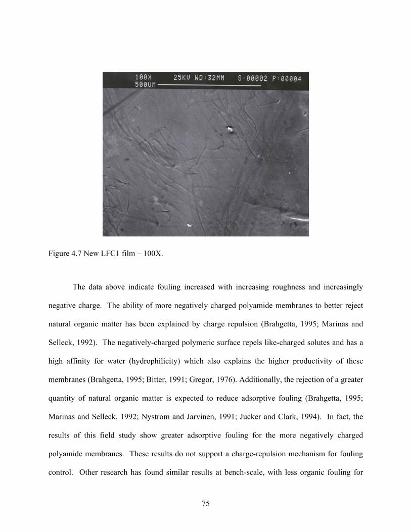
Figure 4.7 New LFC1 film – 100X.
y charged polyamide membranes to better reject
natural organic matter has been explained by charge repulsion (Brahgetta, 1995; Marinas and
Selleck, 1992). The negatively-char pels like-charged solutes and has a
high affinity for water (hydrophilicity) which also
membranes (Brahgetta, 1995; Bitter, 1991; Gregor, 1976). Additionally, the rejection of a greater
Marinas and Selleck, 1992; Nystrom and Jarvinen, 1991; Jucker and Clark, 1994). In fact, the
results of this field study show greater adsorptive fouling for the more negatively charged
polyamide membranes. These results do not support a charge-repulsion mechanism for fouling
Other research has found similar results at bench-scale, with less organic fouling for
The data above indicate fouling increased with increasing roughness and increasingly
negative charge. The ability of more negativel
ged polymeric surface re
explains the higher productivity of these
quantity of natural organic matter is expected to reduce adsorptive fouling (Brahgetta, 1995;
control.
75

cellulos ve de membranes (Nilson and DiGiano, 1996). One possible
explana iffer ace roughness. A rougher film will have a
greater number of sites for adsorption or ion exchange. Polymeric membranes are typically
weak ion-exchange membranes with fixed charge groups commonly provided by sulfonic (SO3-)
and car
The impact of monochloramine addition, flux, and recovery were evaluated by linear
regress e
initial Kw, and a cleaning criterion of 15% producti followed
the form:
e acetate o r polyami
tion is a d ence in surface area, due to surf
boxylic (COO-) functional groups (Brahgetta, 1995; Marinas and Selleck, 1992; Demish
and Pusch, 1976). Regardless of the cause, charge-repulsion by the more negatively charged
membranes did not mitigate fouling but instead these membranes experienced higher fouling
rates than less negatively charged membranes, for this study. Surface roughness correlates with
fouling and may be due to the associated increase in surface area and organic adsorption, as
opposed to increased particle fouling.
Operational Conditions
ion of Kw decline data and calculation of a cleaning cycle based on the decline rate, th
vity decline. The linear regression
K KdK
dttW W
WO
= + (4.2)
Where:
KWO = initial Kw
dKw/dt = rate of change of Kw with time
76

t = time
Average cleaning cycles by o presented in Table 4.4. As shown,
operational times were maximized by 1) addition of a biocide; 2) lower flux; and 3) lower
recovery. The exception to this trend was flux for the CALP, in which case cleaning cycles were
shorter for lower flux rates. This phenomenon may have been due to variations in feed water
quality between the lower and higher flux experiments but is the only exception to this overall
trend. These results show that cleaning frequencies would be minimized by operation at low
flux, low recovery, and with control of biological growth. For individual experiments that were
operated at such conditions, no fouling was observed. This strongly supports the viability of
IMSs for surface water treatment and shows that fouling can be minimized.
perational condition are
Table 4.4 Estimated Effects of Operating Conditions on Nanofilter Cleaning Cycle.
Average Cleaning Cycle (days) Factor Setting 21
CALP ESNA LFC1 No - - 7 Biocide
59 25 13
101 25 7
Recovery
Yes - - 12 7 gfd
(12 L/hr/m2) Flux 14 gfd (25 L/hr/m2)
65% 103 28 16 85% 57 22 7
1 – Experiments that combined the favorable conditions for each factor (biocide addition, low flux, and low recovery) experienced no fouling. 2 – Only tested with CSF pretreatment. Performance of the LFC1 exceeded that of the ESNA when comparing just
CSF pretreatment.
77
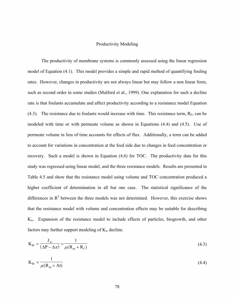
Productivity Modeling
The productivity of membrane systems is commonly assessed using the linear regression
odel of Equation (4.1). This model provides a simple and rapid method of quantifying fouling
rates. However, changes in productivity are not always linear but may follow a non linear form
econd order in some studies (Mulford et al., 1999). One explanation for such a decline
rate is t roductivity according to a resistance model Equation
(4.3). The resistance due to foulants woul e. This resistance term, RF, can be
modeled with time o s shown in Equations (4.4) and (4.5). Use of
permeate volum can be added
to acco
recover n in Equation (4.6) for TOC. The productivity data for this
study was regressed using linear m odels. Results are presented in
Table 4.5 and show that the resistance model using volume and TOC concentration produced a
higher coefficient of deter istical significance of the
differences in R2 between the t dels was not shows
that the resistance m el w y be suitable for describing
Kw. Expansion of resistanc del to inc effects rticles, wth, an er
factors may further support modeling of Kw decl
m
,
such as s
hat foulants accumulate and affect p
d increase with tim
r with permeate volume a
e in lieu of time accounts for effects of flux. Additionally, a term
unt for variations in concentration at the feed side due to changes in feed concentration or
y. Such a model is show
odel, and the three resistance m
mination in all but one case. The stat
hree mo determined. However, this exercise
od ith v and conolume centration effects ma
the e mo lude of pa biogro d oth
ine.
( )KJ
Ww= =
P R Rm f− +∆ ∆π µ1
( ) (4.3)
KR Atm +µ( )W =
1 (4.4)
78
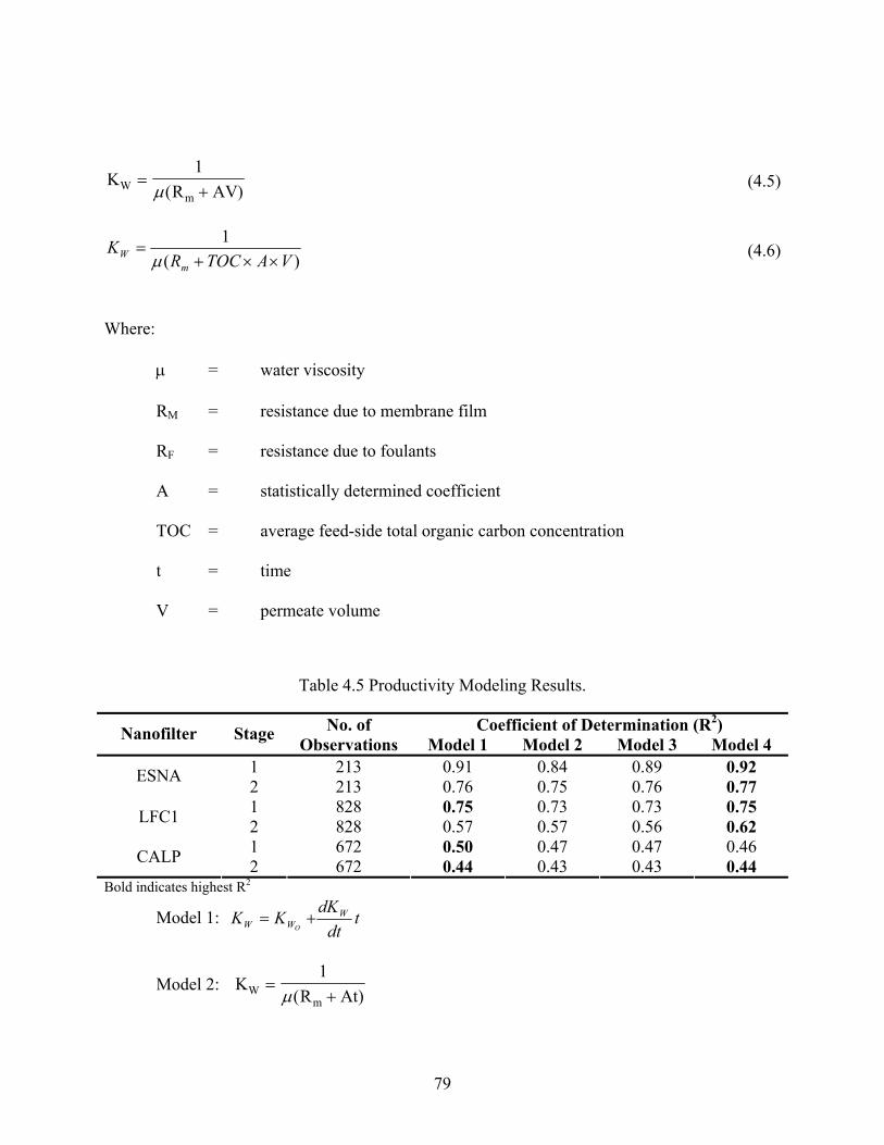
KR AVW
m=
+1
µ( ) (4.5)
)(1
VATOCRK
mW ××+
=µ
(4.6)
Where:
µ = water viscosity
M
F due to foulants
A = statistically determined coefficient
TOC = average tration
t = time
V = permeate volume
R = resistance due to membrane film
R = resistance
feed-side total organic carbon concen
Table 4.5 Productivity Modeling Results.
No. of Coefficient of Determination (R2) Nanofilter Stage Observations Model 1 Model 2 Model 3 Model 4 1 213 0.91 0.84 0.89 0.92 ESNA 6 0.75 0.76 0.77
0.73 0.73 0.75 LFC1 2 828 0.57 0.57 0.56 0.62 1 672 0.50 0.47 0.47 0.46 CALP 2 672 0.44 0.43 0.43 0.44
2 213 0.71 828 0.75
Bold indicates highest R2
Model 1: tdt
dKKK W
WW O+=
KR AtW
m=
+1
µ( ) Model 2:
79
Model 3: KW
R AV=
+1
µ( )
Model 4:
m
)(1
VATOCRm ××+=
µ
WATER QUALITY RESULTS
KW
Water quality samples were obtained every two weeks from both NF systems. Results
are summar in T
As shown, SDS-THMs for the CALP nanofilter were in the range of 34 to 60 µg/L. SDS-
HAA ranged from 1 n sed
US Disinfectant/Disinfection By-Products Rule (D/DBPR) Stage 2 maximum contaminant level
(MCL) of 40 and 3 g fr
disinfectant other than free chlorine or a coagulant-based pretreatment process might be required
to meet the propose
ized able 4.6.
Disinfection By-Product Precursors
9 to 57 µg/L. These results indicate the CALP might ot meet the pro
T
po
hu0 µg/L for THMs and HAAs, respectively, usin ee chlorine. s a
d Stage 2 D/DBP Rule MCLs.
80
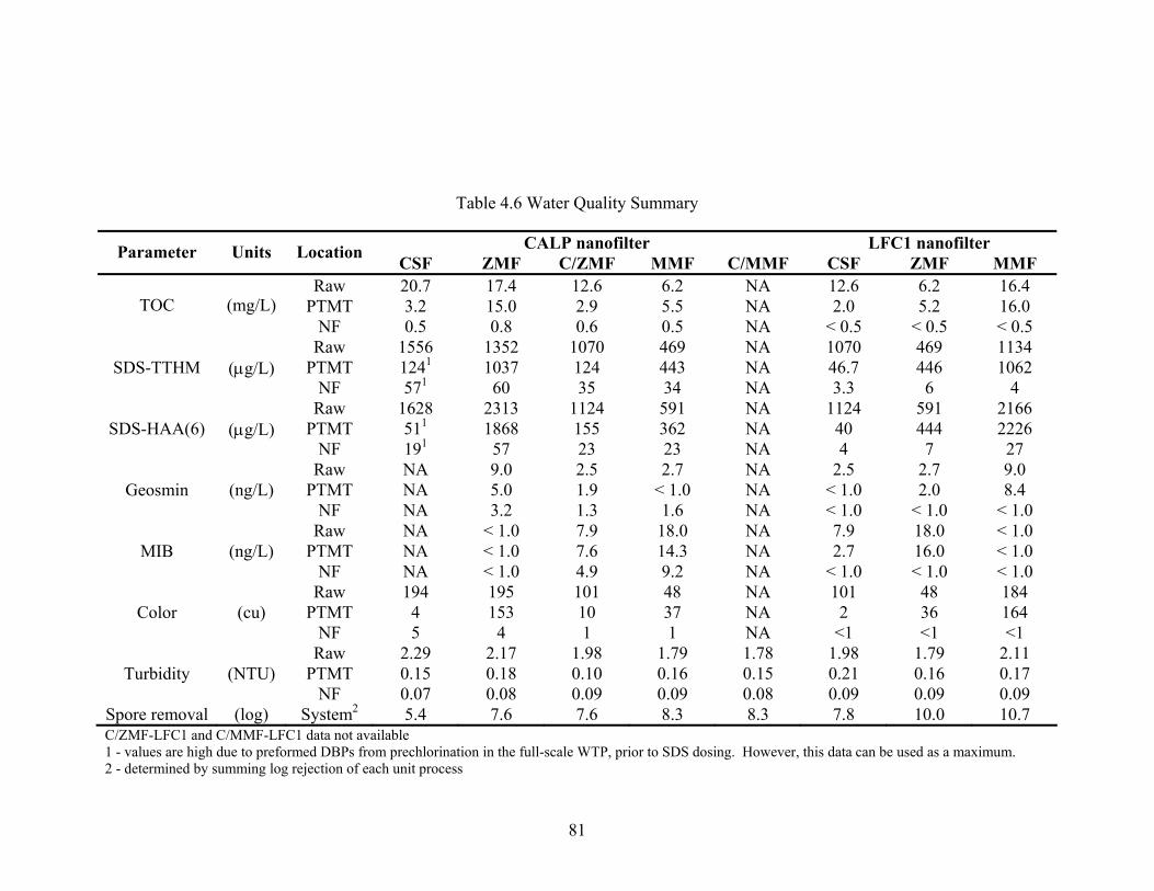
Tabl 4.6 ater Qual y Su mar
filter
e W it m y
CALP nano LFC1 nanofilter Pa e n S Z / F MMF C/MMF MF MF Raw 1 NA 12 6. 16.4
ram ter U its Location C F MF C ZM 20.7 7.4 12.6 6.2
CSF Z M.6 2
PTMT 3. 1 NA 2. 5. 16.0 C g/L) NF 0. 0 NA < 0 0.5
Raw 13 NA 10 46 1134 PTMT 124 10 NA 46 44 1062 SD T g
F 5 6 NA 3. 6 4 Raw 23 A 11 59 2166
M 5 18 A 4 44 2226 gF 1 5 A 4 7 27
Raw N 9 A 2. 2. 9.0 PTMT N 5 A < 1 2. 8.4 G m (ng/
NF N 3 NA < 1 1.0 < NA 7.9 18.0 1.0
M < NA 2.7 16.0 1.0 B (ng/NF N < NA < 1 1.0
Raw 19 1 NA 10 4 184 PTMT 4 1 NA 2 3 164 or (c
NF 5 NA < < <1 Raw 2. 1.78 1. 1. 2.11
PTMT 0. 0.15 0. 0. 0.17 T di (NT NF 0. 0.08 0. 0. 0.09
l (lo System 5. 7 8.3 7. 10 10.7
2 5.0 2.9 5.5 (m5 .8 0.6 0.5
1556 52 1070 469
TO
S-T HM
SDS-HAA(6)
eos in
MI
Col
urbi ty
Spore remova
1 37 124 443 (µ /L) N 71 0 35 34
1628 13 1124 591 PT T 1
NNNNN
1 68 155 362 (µ /L) N 91 7 23 23
A .0 2.5 2.7 A .0 1.9 < 1.0 L)A .2 1.3 1.6
Raw NA 1.0 7.9 18.0 PT T NA 1.0 7.6 14.3 L)
A 1.0 4.9 9.2 4 95 101 48 53 10 37 u) 4 1 1
2.29 17 1.98 1.79 0.15 18 0.10 0.16 U)0.07 08 0.09 0.09
g) 2 4 .6 7.6 8.3
0 2 .5 < 0.5 <
70 9 .7 6 3 24 1 0 4 5 7 .0 0 .0 < 1.0 <
<<
.0 < 1.0 <1 8 6 1 1 98 79 21 16 09 09 8 .0
C/ZM F d C/MM C a vai 1 - va ar h due to orm B o na n ll e , o dosing. However, this dat b d a m. 2 - de in summin r o t es
F-L C1 anlues e higterm ed by
F-LF 1 dat not a lable pref ed D Ps fr m prechlori tion i the fu -scal WTP prior t SDSg log ejecti n of each uni proc s
a can e use as a m ximu
81
82
apable of consistently reducing TOC to
below 0.5 mg/L.
Taste and Odor
MSs removed 40 to 65 percent of geosmin and MIB but
detectable concentrations still remained. The LFC1 IMSs were able to reduce concentrations to
less than the 1 ng/L detection limit in all cases.
It is not clear if the CALP nanofilter could meet taste and odor control requirements.
However, if CSF pretreatment is employed, product water from the CALP would still be lower in
The LFC1 nanofilter, with its lower molecular weight cut-off, is capable of greater
organics rejection. SDS-THM and SDS–HAA values are well below 10 µg/L except for SDS-
HAAs for the MMF-LFC1 system, which average 27 µg/L. Never the less, the LFC1 membrane
would be suitable for meeting Stage 2 regulations and is c
For the Hillsborough River, taste and odor compounds, geosmin (trans-1,10-dimethyl-
trans-9 decanol) and MIB (2-methlyisoborneol), are present during summer months and are
difficult to remove via conventional treatment. Geosmin and MIB are secondary metabolites of
certain blue-green algae and Actinomycetes. The two compounds have stable ring formations
that make bond-cleaving by oxidants difficult. Geosmin and MIB have molecular weights of
approximately 182 and 168 daltons, respectively, which suggests greater removal would be
achieved by the 200 molecular weight cutoff (MWCO) LFC1 nanofilter versus the 300 MWCO
CALP nanofilter. Odor problems associated with both compounds have been reported at levels
as low as 10 ng/L. As shown in Table 4.6, pretreatment processes removed from 5 to 65 percent
of geosmin and MIB. The CALP I

83
MIB and geosmin than the current finished water supply. The LFC1 membrane, with its lower
MWCO, is capable of complete geosmin and MIB removal at the concentrations encountered
and most likely would be able to remove the substantial fraction, if not all, of the taste and odor
compounds which might result in consumer complaints.
Pathogen Rejection
To evaluate the pathogen protection provided by each IMS, challenge testing of unit
processes was performed. Research by the United States Environmental Protection Agency
(USEPA) has shown that bacterial endospores (i.e. Bacillus subtilis) can be used as surrogates
for the protozoans Cryptosporidium and Giardia (Rice et al., 1994). These organisms propagate
in the soil and are ubiquitous in surface waters. The spores are ellipsoidal to spherical in shape
and on average measure approximately 0.5 X 1.0 X 2.0 µm. For the CSF system (full-scale
WTP), log r
7
emoval was determined by measurement of indigenous spore populations. All other
unit processes were challenged with approximately 1X10 cfu/100 ml of Bacillus subtilis
cultured on-site by the Tampa Water Department laboratory. The log rejection of spores for each
unit process was summed by IMS, to provide an estimate of the expected IMS performance.
Results are presented in Figure 4.8.

4
84
5
6
7
CSF-CLP
ZMF-LP
ZMF-LP
MMF-CLP
MMF-LP
CSF-C1
ZMF-C1
C/ZMF-C1
MMF-C1
/MMF-
C1
Sor
e r
8
9
10
12
A CA
C/
CA A
C/
CA LF LF LF LF
C
LF
pem
oval
(log
)
11
1 – Summation of log removals obtained from challenge testing of each unit process.
Figure 4.8 Spore Removal by IMS1.
The order of performance by pretreatment was MMF>ZMF>CSF. The difference in
significant. The order of performance by nanofilter was LFC1>CALP. Thus the IMS capable of
g rejection of spores would be the MMF-LFC1 or the C/MMF-LFC1.
No difference was found between the MF systems with or without in-line coagulation. The CSF
remova
other systems. In summary, the use of multiple barriers for pathogen control is favored by
USEPA and can be accomplished by IMSs. Results of this study show that log rejection of
spore rejection between the MMF and ZMF systems was less than 0.7 log and may not be
providing the highest lo
l capabilities were potentially understated due to the lower spore concentrations found in
the natural surface water compared to the seeded concentration of 1X10⁷ cfu/100 ml used for the
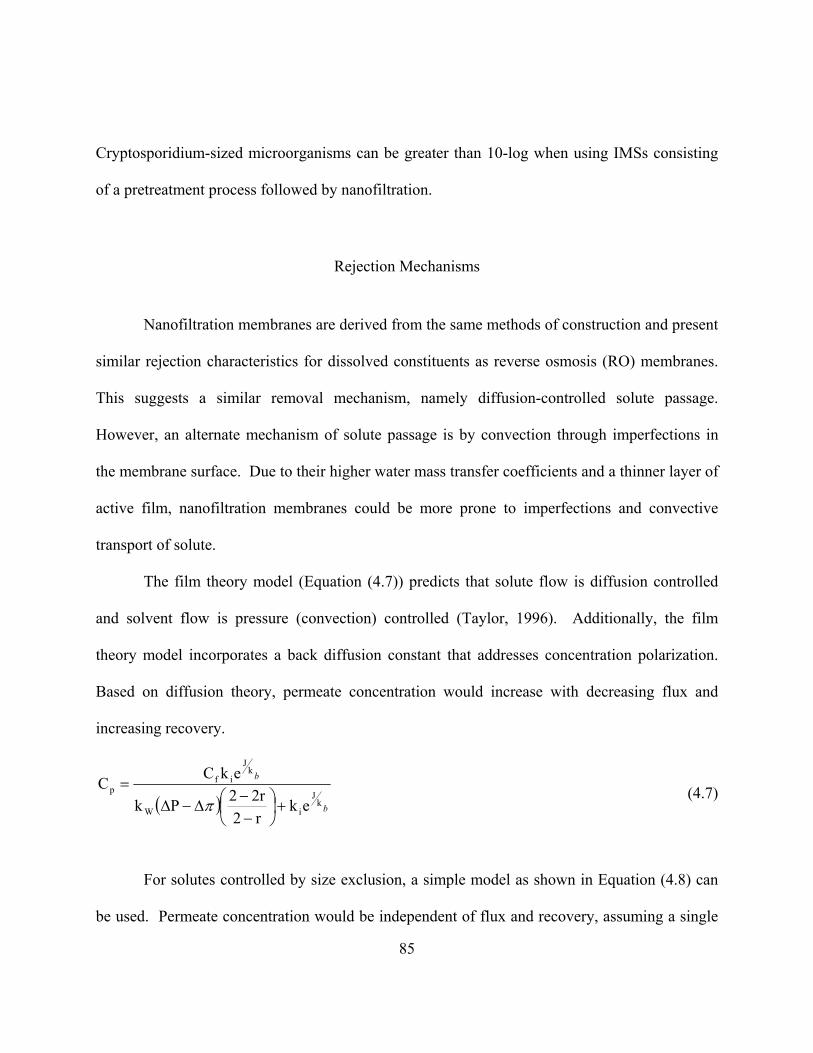
Cryptosporidium-sized microorganisms can be greater than 10-log when using IMSs consisting
of a pretreatment process followed by nanofiltration.
85
Rejection Mechanisms
Na es are derived from the same methods of construction and present
similar j
This sugg
However, an alternate mechanism of solute passage is by convection through imperfections in
the mem r
active film ould be more prone to imperfections and convective
transport of solute.
The film theory model (Equation (4.7)) predicts that solute flow is diffusion controlled
vent flow is pressure (convection) controlled (Taylor, 1996). Additionally, the film
theory m del incorpo nt that addresses concentration polarization.
Based on diffusion theory, permeate concentration would increase with decreasing flux and
increas
nofiltration membran
re ection characteristics for dissolved constituents as reverse osmosis (RO) membranes.
ests a similar removal mechanism, namely diffusion-controlled solute passage.
b ane surface. Due to their higher water mass transfer coefficients and a thinner layer of
, nanofiltration membranes c
and sol
o rates a back diffusion consta
ing recovery.
( ) b
b
iW
if ekC
be used. Permeate concentration would be independent of flux and recovery, assuming a single
kJ
kJ
p
ekr22r2Pk
C+⎟
⎠⎞
⎜⎝⎛
−−
∆−∆=
π (4.7)
For solutes controlled by size exclusion, a simple model as shown in Equation (4.8) can
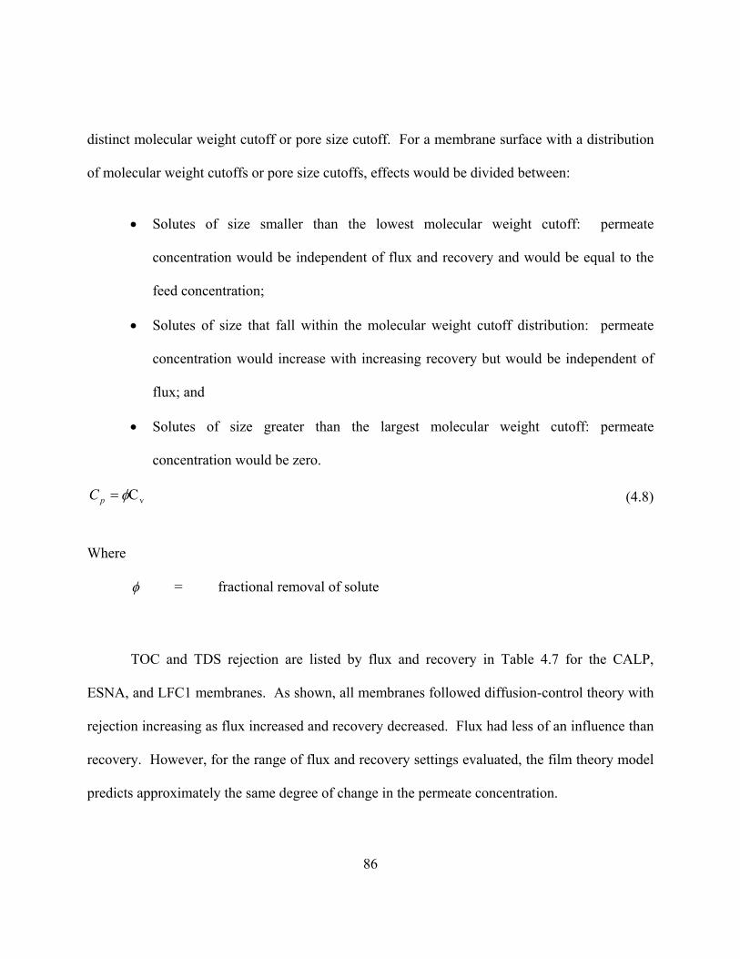
86
distinct molecular w with a distribution
o eight c offs or pore size c ts would be divided
Solutes e smaller than the lowe molecular weight cutoff: permeate
concentrat n would be ind pendent of flux and recovery and would be equal to the
feed concentration;
• Solutes of size that fall within the molecular weight cutoff distribution: permeate
eight cutoff or pore size cutoff. For a membrane surface
f molecular w ut utoffs, effec between:
• of siz st
io e
concentration would increase with increasing recovery but would be independent of
flux; and
• Solutes of size greater than the largest molecular weight cutoff: permeate
concentration would be zero.
vCφ=pC (4.8)
Where
φ = fractional removal of solute
TOC and TDS rejection ar very in Table 4.7 for the CALP,
ESNA, and LFC1 membranes. As shown, all membranes followed diffusion-control theory with
rejectio
e listed by flux and reco
n increasing as flux increased and recovery decreased. Flux had less of an influence than
recovery. However, for the range of flux and recovery settings evaluated, the film theory model
predicts approximately the same degree of change in the permeate concentration.

87
Table 4.7 TOC and TDS Rejection by Flux and Recovery.
Parameter Flux (gfd) Recovery (%) Membrane 7 14 65 85
TOC CALP 93 94 96 93
LFC1 96 96 97 96
TDS CALP 37 49 45 37
LFC1 90 89 94 85
ESNA 94 97 97 94
ESNA 86 98 99 86
The diminished influence of flux that was observed may have been due to partial
convective passage of solute as suspected in NF systems. The impact of varying flux and
recovery on TDS rejection was much greater than on TOC rejection. The average molecular
weight of compounds that make up TDS may be smaller than that of TOC compounds, which
would explain this difference. The conclusion from this evaluation is that both diffusion and size
exclusi
Size exclu igher molecular weight constituents such as those
present
In summary, the IMSs using the CALP nanofilter are suitable for meeting current US
regulations. Long term regulatory compliance with the CALP nanofilter would be more readily
met by selecting a pretreatment process that uses a coagulant, such as CSF, or via the use of a
disinfectant other than free chlorine. The coagulant would remove a portion of TOC, taste &
on mechanisms play a role in control of solute passage, for these three NF membranes.
sion has a greater impact on h
in TOC.
Water Quality Summary

88
odor co p
Never the s a water higher in quality than most conventional
treatme s
current or atment process. Decisions regarding
selectio o
driven by
exclusion.
m ounds, and other constituents that the CALP nanofilter is only partially able to reject.
less, the CALP nanofilter produce
nt ystems, for the source water tested. The LFC1-based IMSs are capable of meeting
proposed US regulations irrespective of the pretre
n f a pretreatment process to pair with the LFC1 membrane would most likely be solely
cost. Rejection for all three membranes was influenced by diffusion and size
CONCLUSIONS
Productivity
• The order of membrane fouling, from most to least fouling, was
ESNA>LFC1>CALP.
• The CALP system requires addition of an oxidant such as monochloramines to
control biological degradation of the membrane film.
• The CALP system required no chemical cleanings over a 6-month period. The 10
percent decline in Kw observed was independent of pretreatment process and
operating conditions.
• Projected CALP nanofilter cleaning frequency is once every 9 months.
• The ESNA irreversibly fouled and was not a viable membrane for this source.
89
• Bacterial growth contributed g; cleaning cycles were improved with
the addition of monochloramine.
• The LFC1 suffered damage due to oxidation from the monochloramine and would
need a non oxidative biocide for use at this site.
• The order of membrane surface charge, from most to least negative, as well as surface
roughness, from most to least rough, was ESNA>LFC1>CALP, which followed the
order of fouling.
• A more negatively charged membrane surface correlated with increased fouling,
indicating electrostatic repulsion was not effect for fouling control. Increased surface
area, due to greater surface roughness, for the more negatively charged membranes
may have contributed to organic adsorption fouling.
• Fouling was reduced with addition of monochloramine, lower flux, and lower
recovery. Experiments operated under such conditions did not foul and affirmed the
• Statistical regression of productivity decline data showed that a resistance model
using permeate volume and TOC concentration better fit Kw decline data than the
linear model and other less complex resistance models. Further development of the
resistance model is recommended.
to LFC1 foulin
viability of IMSs for treatment of this source.

90
•
MF treatment.
•
• nanofilter can meet Stage 2 regulations with any of the pretreatment
•
found to be a function of pretreatment unit as well as nanofilter. Spore
cap The MF systems outperformed CSF and the LFC1 nanofilter
• Org and size
by
Water Quality
• MF can remove significant amounts of particles, turbidity, and pathogens and can not
reject color, DBPFP or DOC unless augmented by another process.
The nanofiltration systems provide a higher quality water, compared to conventional
coagulation treatment (CSF) or
• The LFC1 nanofilter provided a higher quality permeate than the CALP nanofilter.
This can be attributed to the composition and lower MWCO of the LFC1 compared to
the CALP.
The CALP nanofilter can meet current and Stage 1 D/DBPR regulations. Stage 2
regulations may require a coagulant-based pretreatment or an alternate disinfectant.
The LFC1
processes evaluated.
Log removals of the sporulated-form of the pathogen surrogate Bacillus subtilis by
IMSs was
removal of the least capable IMS averaged 5.4 log compared to 10.7 log for the most
able system.
outperformed the CALP nanofilter.
anic and inorganic rejection were influenced by both diffusion-
exclusion-mechanisms. Higher molecular weight compounds were controlled more
size exclusion.
91
• Control of biogrowth is crucial for many surface water nanofiltration systems. This
may include addition of oxidants such as monochloramine or control of dissolved
oxygen by methods such as limiting exposure to the atmosphere or addition of
oxygen scavenging chemicals.
• The ability of a given membrane to withstand extended exposure to monochloramine,
other oxidants or any other non standard chemical should be thoroughly investigated
to ensure long term membrane viability. Six to twelve months or more of pilot
operation may be required for any integrity losses to become evident. The membrane
warranty should reflect anti atment methods including addition of
oxidants.
• Fouling rates and finished water quality are dependent on membrane make and
model, raw water quality, operational conditions, and system design. To ensure goals
are met:
Long-term testing (> 6 months) of the selected membrane make and model should
be conducted.
The raw water quality should be representative of that which will be fed to the
full-scale plant. Seasonal variations should be included in the testing.
The pilot design should reflect all unit processes expected in the full-scale system,
including pretreatment processes, pretreatment chemicals and doses, static
prefilters, and acid, antiscalent, and bioinhibitor type and dose.
Pilot and Full-Scale Design Considerations
cipated pretre

92
Operational conditions ( ry) should be tested to the limits of
expected settings.
. A
ane that becomes irreversibly fouled and requires
• The benefit of a low fouling cellulose acetate membrane must be weighed against the
SUMMARY
flux and recove
• The ability to restore membrane productivity, once fouled, must be determined
laboratory or pilot study that does not evaluate the ability to clean a fouled membrane
may allow selection of a membr
replacement at full-scale.
potential for damage or destruction via biodegradation or hydrolysis.
This pilot study has shown nanofiltration of the Hillsborough River to be viable in terms
treatment, source water quality issues as well as future regulations are causing many utilities to
n and
of water quality and membrane system operation. Though more expensive than conventional
consider alternative technologies. For rejection of high concentrations of organic matter, taste &
odor compounds, pathogens, and many other constituents, nanofiltration is an effective process.
Additional research is needed for fouling mechanism identification and fouling mitigatio
would support the use of nanofiltration for surface water treatment.
93
REFERENCES
Bitter, J. G., 1991. Transport Mechanisms in Membrane Separation Proceses, Plenum Press.
Braghetta, A., 1995. The Influence of Solution Chemistry and Operation Conditions on Nanofiltration of Charged and Uncharged Organic Macromolecules. Doctoral dissertation, University of North Carolina at Chapel Hill.
Demish, H.U. and Pusch, W, 1976. “Ion Exchange Capacity of Cellulose Acetate Membranes”, J. Electrochemistry Society, 123:3 370-374
Gregor, H.P., 1976. Fixed-Charge Ultrafiltration Membranes, in Charge Gels and Membranes, Part 1, ed. E. Selegny, 57-69.
Jucker, C. and Clark, M.M., 1994. Adsorption of Aquatic Humic Substances on Hydrophobic Ultrafiltration Membranes, J. Membrane Science, 97, 37-52.
Marinas, B. and Selleck, R.E., 1992. “Reverse Osmosis Treatment of Multicomponent Electrolyte Solutions, J. Membrane Science, 72, 211-229.
Mulford, L.A., Tram, Q., and Taylor, J.S., Feb. 1999. “Modeling and Performance Evaluation of a Groundwater Nanofiltration Plant”, Proceedings of the AWWA Membrane Technology Conference, Long Beach, CA.
Nilson, J.A., and DiGiano, F.A., May 1996. “Influence of NOM Composition on Nanofiltration” J. Am. Water Works Assoc., 88:5:53.
Nystrom, M. and Jarvinen, P., 1991. Modification of Polysulfone Ultrafiltration Membranes with UV Irradiation and Hydrophilicity Increasing Agents, J. Membrane Science, 60, 275-290.
Reiss, C.R., Taylor, J.S., and Mulford, L.A., Mar. 1996."Comparison of Surface and Groundwater Membrane Pilot-Scale Investigations", Proceedings AWWA GAC, Membranes & the ICR - A Workshop on Bench-Scale and Pilot-Scale Evaluations, Cincinnati, OH.
Reiss, C.R. and Taylor, J.S., Mar. 1991. “Membrane Pretreatment of a Surface Water” Proceedings AWWA Membrane Specialty Conference, Orlando, FL.
94
Rice cal surro ater Quality Technolo
Taylor, J.S, 1996. Reverse Osmosis and Nanofiltration, in Water Treatment Membrane Processes, ed. P. Jacobs, et al., McGraw
, E.W., Fox, K.R., Miltner, R.J., Lytle, D.A., and Johnson, C.H., 1994. A microbiologigate for evaluating treatment efficiency.“ American Water Works Association W
gy Conference, San Francisco, CA, November 6-9.
-Hill, NY.
95
INTRODUCTION
CHAPTER 5 MONOCHLORAMINATION PRETREATMENT FOR NANOFILTRATION MEMBRANE PROCESSES
urface waters for potable water production has increased significantly in the
United States due to depletion of pristine g
The use of s
round source waters. However, the surface waters
typically have a wide spectrum of contaminants and their treatment is more strictly regulated by
various water quality rules (Taylor et al, 2000). Increasingly stringent water quality regulations
for surface waters have prompted an interest in membrane technologies such as reverse osmosis
(RO) and nanofiltration (NF) (Reiss et al, 1999). However, the problems with membrane
fouling, in conjunction with consequent feed water pretreatment difficulties, have hampered the
wide acceptance of membrane processes as a treatment of choice for surface waters (Hong et al,
1997).
Among numerous fouling mechanisms, biological fouling is considered to be one of the
most common and recalcitrant operational problems in surface water treatment (Reiss et al, 1999;
Saeed, 2002). The importance of biofouling control in membrane processes has been recognized
in many studies of membrane systems (Bergman et al, 1997; Duranceau et al, 1998; Hafsi et al,
2004). Kruithof found river water containing high concentrations of iron and manganese could
not be successfully pretreated for membrane treatment due to biological fouling (Kruithof et al,
1997). Successful pretreatment (cleaning frequencies > 6 months) were achieved by injecting
the river water via Raney wells into the aquifer to achieve an anaerobic state. Studies at

96
Amster
olymers and
compro
sms in the raw water, it does not allow exposure of the NF or
O membrane film to the biocide for control of attached biological growth. The availability of
an oxidant-resistant membrane combined with the high performance characteristics typical of PA
membranes is of importance and would increase the applications available to membrane
technology.
dam Water Supply Company (AMS), using river water pretreated by coagulation-
sedimentation-filtration (CSF) found that BaSO4 scaling could be controlled using antiscalent,
but the assimilable organic carbon (AOC) content of the antiscalent was too high to prevent
biofouling. Biofouling control was achieved by using acid for RO pretreatment that had very
low AOC.
Despite some success of alternative methods for biofouling control at pilot-scale, a
commonly practiced means for alleviating biofouling is the addition of biocides. Biocides are
continuously or intermittently injected to feed water in order to prohibit microbial growth in the
membrane system. The use of chlorine, the most widely used disinfectant in drinking water
industry, however, is not desirable because it interacts with membrane p
mises the integrity of the membrane structure (Glater et al, 1994; Peterson, 1993;
Avlonitis et al, 1992; Lowell et al, 1987; Kawaguchi et al, 1984; Glater et al, 1983). In
particular, thin film composite polyamide membranes show extreme sensitivity to feed water
chlorination. The performance of these membranes deteriorates severely even at low levels of
chlorine exposure. As a result, biological control of polyamide membranes typically involves
addition of a chlorine-based oxidant in the raw water and quenching of the residual before
entering the membrane pressure vessels (Saeed, 2002; Hafsi et al, 2004). While this method
inactivates most viable microorgani
R

97
Monochloramine (NH2C as a membrane system biocide
because of its lower oxidation-reduction potential and would therefore be less aggressive toward
membrane films. Monochloramine is for tion of ammonia with aqueous chlorine,
typically at a Cl :N ratio of 4 (US EPA, 1999; Connell, 1997). It has been recognized that
monochloramine in water distribution systems can be effective for controlling bacterial growth.
Furthermore, it forms much less disinfection by products (DBPs) than chlorine. Several studies
have demonstrated membrane degradation issues associated with use of chloramination but have
Seamans et al, 2003). Despite its increasing application, extensive and/or systematic studies on
the interaction of monochloramine with various NF or RO membranes are limited.
The main goal of this study was to investigate the effect of monochloramine on NF
membrane performance during the treatment of high organic surface water. Two types of
embranes, made of cellulose acetate and polyamide, were evaluated.
Following 15 months of pilot operation, membrane autopsies were performed and chemical
changes in the NF mem ition, a series of well-
controlled bench-scale experiments were performed to validate pilot-scale observations. Lastly,
the p echanisms of l interactions n the selec amide mem and
monochloramine were delin
l) has a greater potential for use
med by the reac
2
not identified the mechanisms of chemical attack to the membrane film (Alvarez et al, 2003;
commercial NF m
branes were identified by XPS and FTIR. In add
ossible m chemica betwee ted poly brane
eated.

98
EXPER HODSIMENTAL MET
, the total
organic carbon (TOC) ranged from 4 to 28 mg/L, total hardness from 50 to 180 mg/L as CaCO3,
and alkalinity from 30 to 1 r quality parameters were
monitored biweekly for this period, and the results are prese
n es a of s gi to
system
.1 H roug Water Quality
Parameter Units Maximum Minimum Average
Source Water
The source water used in pilot study was the Hillsborough River in Tampa, Florida.
Water quality varies greatly between the wet (summer) and dry (winter) seasons. During the wet
season, storm water traveling through marsh areas brings highly organic fresh water to the river
and reduces hardness and alkalinity. Conversely, the dry season is characterized by lower
organic levels and higher hardness and alkalinity. During 15 months of operation
80 mg/L as CaCO3. A variety of wate
nted in Table 5.1. Owing to high
evere bioloorganic conte t, this source water impos great risk cal fouling an NF
.
Table 5 illsbo h River Raw
UV-254 (cm-1) 0.151 0.741 1.907
TOC (mg/L) 27.5 4.0 16.4
Particle Count (#/ml, >2.0 um) 62,608 1,479 12,234
Alkalinity (mg/L as CaCO3) 178 30 80
Total Hardness (mg/L as CaCO3) 184 50 108
TDS (mg/L) 270 63 169
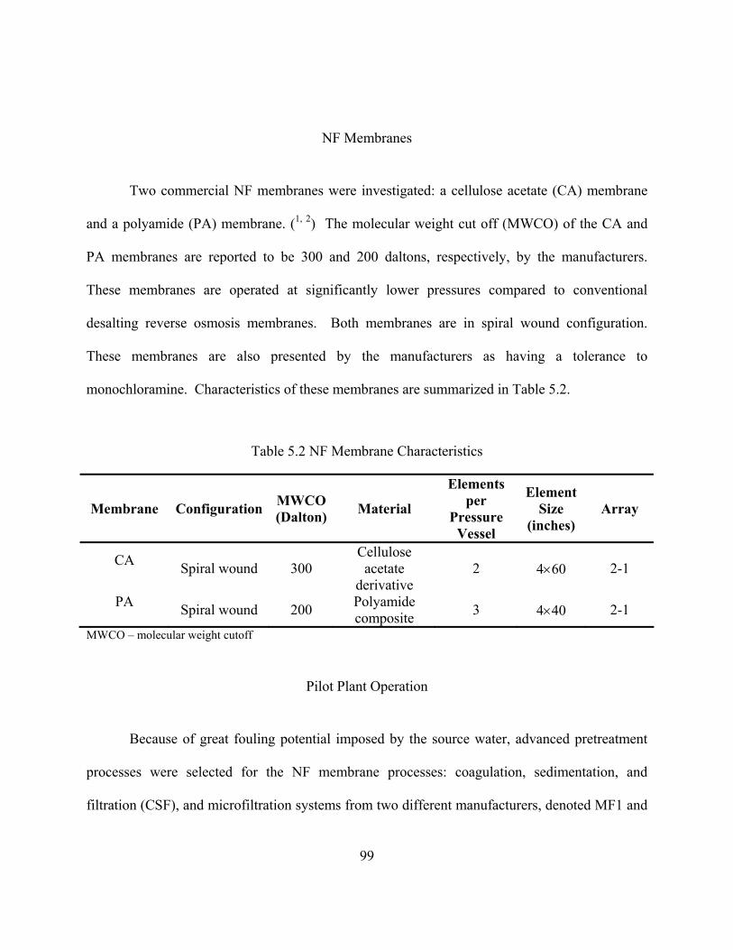
99
Two commercial NF membranes were investigated: a cellulose acetate (CA) membrane
and a polyamide (PA) membrane. (1, 2) The molecular weight cut off (MWCO) of the CA and
PA membranes are reported to be 300 and 200 daltons, respectively, by the manufacturers.
These membranes are operated at significantly lower pressures compared to conventional
desalting reverse osmosis membranes. Both membranes are in spiral wound configuration.
These membranes are also presented by the manufacturers as having a tolerance to
monochloramine. Characteristics of these membranes are summarized in Table 5.2.
Table 5.2 NF Membrane Characteristics
Elements
NF Membranes
Membrane Configuration MWCO(Dalton) Material per
Pressure Vessel
Element Size
(inches) Array
CA Spiral wound 300 acetate 2 4×60 2-1
Cellulose
derivative PA Spiral wound 200 Polyamide 3 4×40 2-1 composite
MWCO – molecular weight cutoff
Pilot Plant Operation
d MF1 and
Because of great fouling potential imposed by the source water, advanced pretreatment
processes were selected for the NF membrane processes: coagulation, sedimentation, and
filtration (CSF), and microfiltration systems from two different manufacturers, denote

100
MF2. (
te coagulation, sedimentation, and sand filtration. The raw
water drawn from Hillsborough River was dosed with ferric sulfate at an average of 170 mg/L.
Since the plant employed prechlori hlorine was present in the filtrate
and was removed via granular activated carbon (GAC) filtration. The filter had been exhausted
of TOC removal capacity, to prevent further organic matter removal by GAC. TOC and chlorine
residuals were monitored weekly from the GAC column. Following the four-month period of
TOC exhaustion, the GAC column removed less than 0.1 mg/L of TOC and continued to reduce
the free chlorine residual to below detection.
The two NF pilot plants were 2-1 array systems with 120 inches of membrane length per
vessel. The PA and CA membranes were independently tested in separate, parallel pilot
units. NF fluxes of 11.9 and 23.8 lmh (7 and 14 gfd) and recoveries of 65 and 85 percent were
specifie taling 8 weeks of operation, for each pretreatment
process. Conc rate to accommodate the specified recoveries.
3, 4) Furthermore, the MF1 and MF2 systems were also tested with the addition of in-line
coagulation, denoted C/MF1 and C/MF2.
Both the MF1 and MF2 microfiltration systems are made of hollow fibers with a nominal
pore size of 0.1 and 0.2 µm, respectively. The MF1 and MF2 systems consisted of pilot-scale
units installed at the City of Tampa’s David L. Tippen Water Treatment Plant (DTL WTP) site.
The MF1 unit is capable of producing 3.15 to 7.56 x 10⁻⁴ m3/s (5 to 12 gpm) of filtrate. The MF2
unit produces 5.04 to 18.9 x 10⁻⁴ m3/s (8 to 30 gpm) of filtrate.
The CSF water was obtained from the DLT WTP in Tampa, Florida. This surface water
treatment plant utilized ferric sulfa
nation, a residual of free c
pressure
d for a total of four experiments to
ent recycle was utilized

101
ystem. After
experie
Performance Evaluation
he performance of the NF membranes was monitored in terms of productivity and
rejection. The memb uantified by measuring the water mass transfer
coefficient, Kw
Filtrate from the MF1, MF2, and CSF processes was pumped to the NF systems where
hydrochloric acid and/or antiscalent (AS) were added. (5) The hydrochloric acid was added at a
dose sufficient to prohibit calcium carbonate scaling and minimize CA membrane hydrolysis.
When used, a target pH of 5.5 was maintained. The antiscalent was dosed at 2.5 mg/L for 85
percent recovery and 5.0 mg/L for 65 percent recovery to prohibit iron fouling. Antiscalent dose
was increased with decreasing recovery as dictated by antiscalent manufacturer computer
projections, to maintain target levels of antiscalent in the concentrate of the NF s
ncing performance issues with both the CA and PA membranes, monochloramine was
added to the feed water at 5 mg/L.
T
rane productivity was q
:
( )π∆−∆=
PJ
K Ww (5.1)
Where
Jw = water flux
∆P = pressure gradient
∆π = osmotic pressure

To identify membrane performance deterioration events, such as fouling and degradation,
a linear regression of Kw with time was performed to determine the slope or rate of change.
Fouling is characterized by a decrease in Kw, indicating a reduced flow and/or increased pressure
requirement. Degradation represents a loss of membrane integrity (e.g. structural failure) and is
characterized by an increase in Kw. This indicates increased flow and/or a lower pressure
requirement. Typically an NF system is chemically cleaned following a 10 to 15 percent decline
in Kw. A common goal for cleaning frequency is no more than once per 6 months.
102
In addition to productivity, the capability of NF membranes to reject total dissolve solid
(TDS) was monitored to identify dation or loss of integrity would
be characterized by a decrease in rejection. The equation for TDS rejection (R) is:
membrane degradation. Degra
CCf
−
In order to further study the effect of monochloramina
CR pf= (5.2)
Where
Cf = feed TDS concentration
Cp = permeate TDS concentration
Bench Scale Monochloramine Exposure Experiment
tion on polyamide membranes, the
PA membrane was exposed to varying doses of monochloramine (0 to 50 mg/L) for a period of
two weeks (Beverly, 2000). The monochloramine stock solution (500 mg/L) was first prepared
using ammonium chloride and sodium hypochlorite in deionized (DI) water. Membrane sections

103
were cut from flat sheets of m was placed in a separate leak-
proof, chemical resistant Nalgene bottle. The monochloramine-spiked solution was then added
to fill the bottle. The m solution under a fume
hood for two weeks. Monochloramine concentration was measured throughout the experiment
using a titrimetric method as outlined in Standard Methods (Standard Methods, 1996). The
standardized reagent solutions were used in these measurements. All chemicals were used
within two weeks of opening and unused portions were discarded according to regulations.
lowed to dry under vacuum
before
embrane material. Each section
embranes were soaked in the monochloramine
Membrane Surface Analysis
For each membrane, new and used samples were tested and compared by X-ray
Photoelectron Spectroscopy (XPS) (Beverly et al, 2000; Briggs, 1998; Seal et al, 1997; Beamson
et al, 1992). Each sample was thoroughly rinsed in DI water and al
analysis. A baseline spectrum of each sample was taken before use to identify any
changes that the membrane had undergone while in use. All XPS analysis was performed using
a XPS spectrometer. (6) In order to verify XPS results, a Fourier Transform Infrared (FTIR)
spectrometer was used to scan new and used membrane samples. (7) All samples were prepared
by separating the active layer and support layers. Detailed procedures of XPS and FTIR analyses
have been presented by Beverly et al. (Beverly et al, 2000).
104
RESULTS AND DISCUSSION
Effect of Monochloramine on CA Membrane
Variations in water mass transfer coefficient over time during the operation of CA
membrane are shown in Figure 5.1. The pilot operation first began using CSF feed water from
the full-scale plant. During operation with CSF feed water, no fouling was observed and
productivity was consistent. Following execution of the CSF experiments, the feed water was
changed to MF1 microfiltered water. Neither the CSF or MF1 feed waters were dosed with
monochloramine. At seven days of operation using MF1 feed water, the Kw increased
dramatically as shown in Figure 5.1 and TDS rejection fell to zero, indicating complete loss of
membrane integrity. The same loss of integrity was experienced at 7 days of operation when a
new set of membranes was installed and is also shown in Figure 5.1.
Suspecting either biodegradation or hydrolysis as the reason for loss of membrane
t CA system with and without acid and
monochloramine addition. Heterotrophic plate counts (HPCs) were monitored for
characterization of bioactivity as shown in Table 5.3. Productivity results are shown in Figure
5.2. Integrity was lost at 10 days of operation without monochloramine or acid addition. In
addition, HPC concentrations were approximately 103 cfu/ml in the feed compared to 105 cfu/ml
and 105.7 cfu/ml in the permeate and concentrate, respectively. This showed biodegradation to be
the cause of failure as opposed to hydrolysis of the membrane. The success of the pH-adjusted
integrity, tests were performed using a single elemen
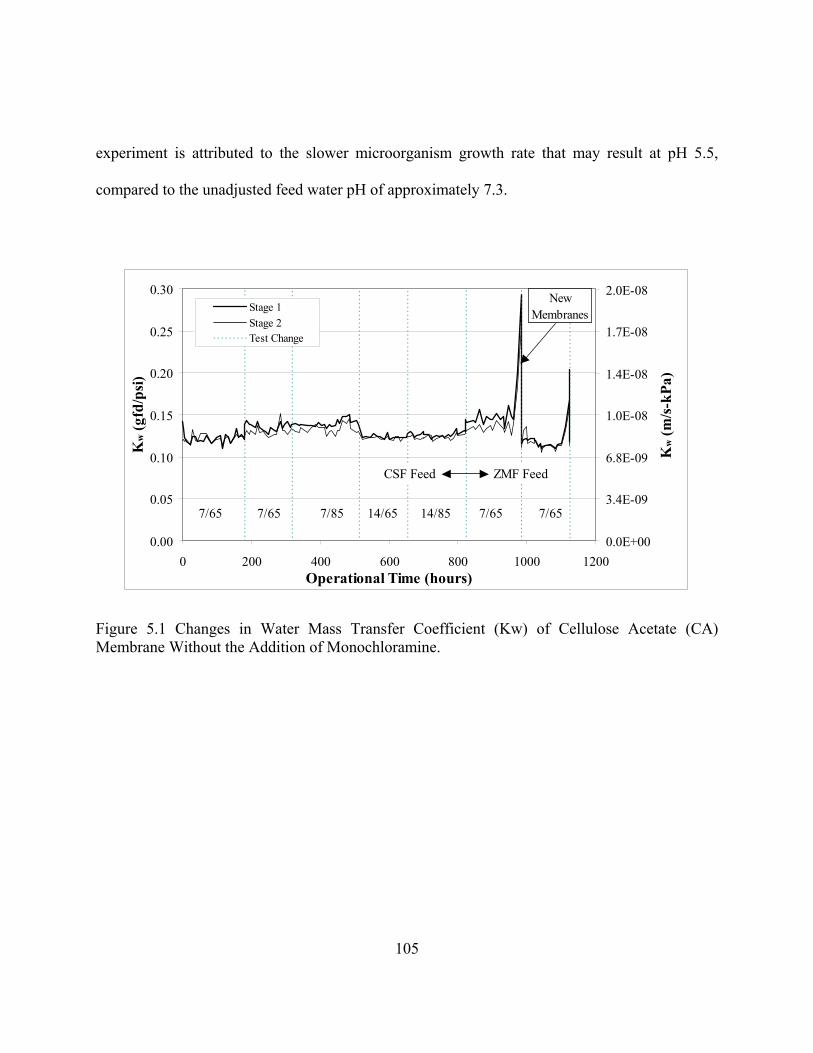
105
experiment is attribu y result at pH 5.5,
compared to the unadjusted feed water pH of approximately 7.3.
ted to the slower microorganism growth rate that ma
0.00
5
.10
.15
.20
.25
0
0 2 400 600 12Operatio al Time (h )
wfd
)
00
09
9
08
8
-08
8
Kw (m
/s-kP
a)
0.0
0
K
0
(g
0
0
0.3
00 800ours
1000 00n
/psi
0.0E+
3.4E-
6.8E-0
1.0E-
1.4E-0
1.7E
2.0E-0Stage 1Stage 2Test Change
7/65 /65 7/85 65 1 7/65 7/65
Newmbranes
CSF Fee ZMd F Feed
7 14/ 4/85
Me
Figure 5.1 Changes in Water Mass Tr nsfer C t (K Cellu cetate (C ) Mem e Without the Addition of Monochloramin
a oefficien w) of lose A Abran e.

106
Table 5.3 HPCs During Single Element CA Operation
Pretreatment HPC
Operational NH2Cl
(hours)
Monochloramine Adjustment
(cfu/ml) (cfu/ml) (cfu/ml) (mg/L)
Time Feed Permeate Concentrate residual in
permeate
pH
to pH 5.5
15 X X 6,600 5,700 1,610 0.6
130 X X 2,500 130 400 0.7
178 X X 13,400 80 11,050 0.8
224 X 7,850 116 9,200 -
290 X 1,260 70 3,100 -
X 2,565 2,807 18,200 -
49
335 X 11,400 915 15,400 -
383
5 X 4,090 31 4,770 0.8
543 X 2,340 5 1,270 0.7
590 X 510 52 6,250 0.9
639 X 222 330 2,100 0.6
784 15,000 316 3,900 -
832 5,110 520 16,200 -
945 323 86 4,340 -
993 2,650 5,300 5,300 -
1,016
880 163 265 4,100 -
1,935 30,000 2,360 -
1,040 5,100 16,700 20,000 -
1,112 1,095 125,500 522,000 - HPC – heterotrophic plate count
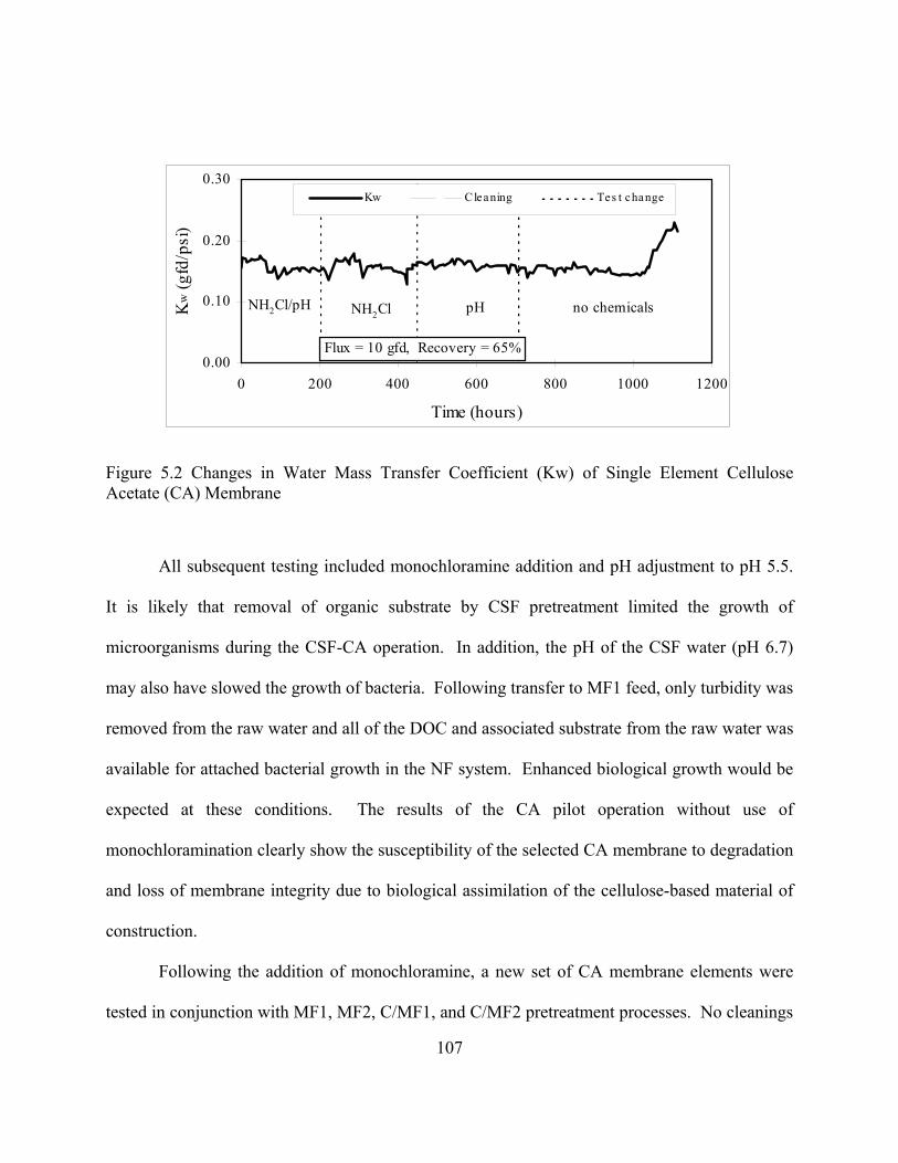
0.00
0.10
0.20
0.30
0 200 400 600 800 1000 1200
Time (hours)
Kw
(gfd
/psi
)Kw Cleaning Tes t change
Flux = 10 gfd, Recovery = 65%
NH2Cl/pH NH2Cl pH no chemicals
Figure 5.2 Changes in Water Mass Transfer Coefficient (Kw) of Single Element Cellulose Acetate (CA) Membrane
All subsequent testing included monochloramine addition and pH adjustment to pH 5.5.
It is likely that remova limited the growth of
microorganisms during the CSF-CA operation. In addition, the pH of the CSF water (pH 6.7)
may als
integrity due to biological assimilation of the cellulose-based material of
construction.
Following the addition of monochloramine, a new set of CA membrane elements were
tested in conjunction with MF1, MF2, C/MF1, and C/MF2 pretreatment processes. No cleanings
l of organic substrate by CSF pretreatment
o have slowed the growth of bacteria. Following transfer to MF1 feed, only turbidity was
removed from the raw water and all of the DOC and associated substrate from the raw water was
available for attached bacterial growth in the NF system. Enhanced biological growth would be
expected at these conditions. The results of the CA pilot operation without use of
monochloramination clearly show the susceptibility of the selected CA membrane to degradation
and loss of membrane
107
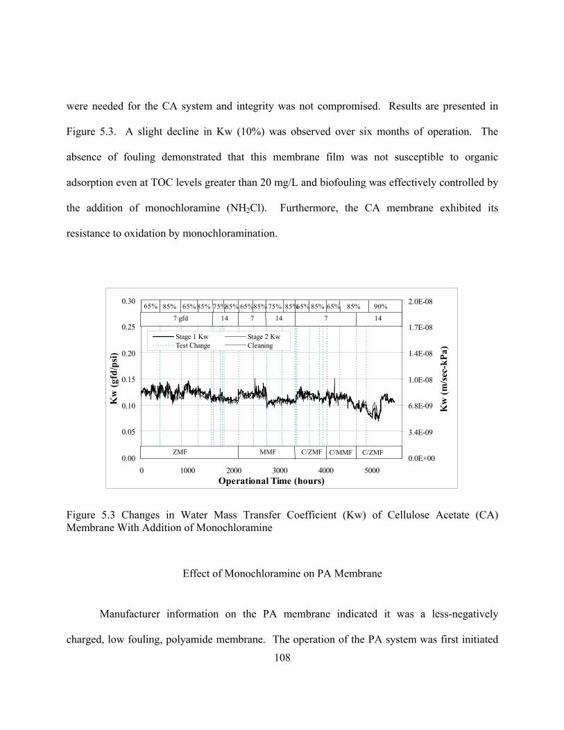
were needed for the CA system and integrity was not compromised. Results are presented in
108
Figure 5.3. A slight decline in Kw (10%) was observed over six months of operation. The
absence of fouling demonstrated that this membrane film was not susceptible to organic
adsorption even at TOC levels greater than 20 mg/L and biofouling was effectively controlled by
the addition of monochloramine (NH2Cl). Furthermore, the CA membrane exhibited its
resistance to oxidation by monochloramination.
0.00
0.05
0.10
0.15
0.20
0.25
0.30
0 1000 2000 3000 4000 5000Operational Time (hours)
Kw
(gfd
/psi)
0.0E+00
3.4E-09
6.8E-09
1.0E-08
1.4E-08
1.7E-08
2.0E-08
Kw
(m/se
c-kP
a)
Stage 1 Kw Stage 2 KwTest Change Cleaning
ZMF MMF C/ZMF C/MMF C/ZMF
65% 85% 65% 85% 75% 65%85% 75%85% 85%65% 85% 65% 90%85%
7 gfd 14 7 14 7 14
Figure 5.3 Changes in Water Mass Transfer Coefficient (Kw) of Cellulose Acetate (CA) Membrane With Addition of Monochloramine
Effect of Monochloramine on PA Membrane
eration of the PA system was first initiated
Manufacturer information on the PA membrane indicated it was a less-negatively
charged, low fouling, polyamide membrane. The op
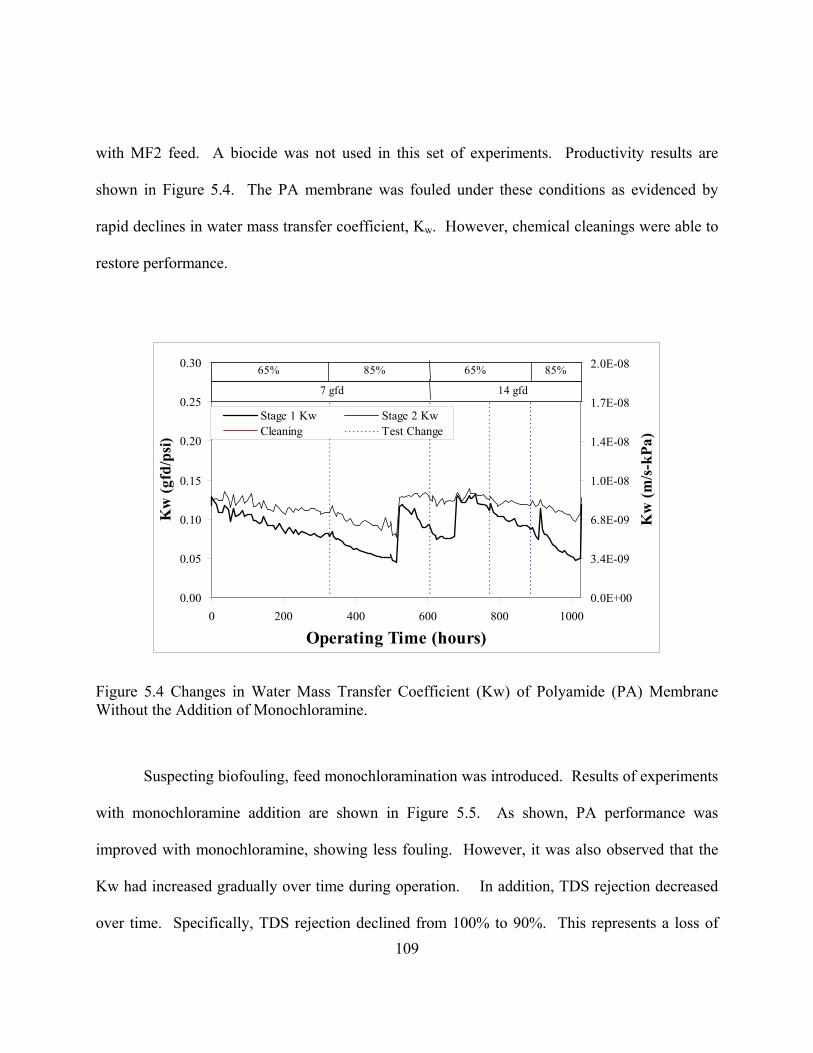
109
with MF2 feed. A biocide w nts. Productivity results are
shown in Figure 5.4. The PA membrane was fouled under these conditions as evidenced by
rapid declines in water mass transfer coefficient, Kw. However, chemical cleanings were able to
restore performance.
as not used in this set of experime
0.00
0.05
0.10
0.15
0.20
0.25
0.30
Kw
(fd
/p)
1.0E-08
1.4E-08
1.7E-08
2.0E-08
Kw
(/s-
ka)
0 200 400 600 800 1000
Operating Time (hours)
gsi
0.0E+00
3.4E-09
6.8E-09
mP
Stage 1 Kw Stage 2 KwCleaning Test Change
65% 85% 65% 85%
7 gfd 14 gfd
Figure 5.4 Changes in Water Mass Transfer Coefficient (Kw) of Polyamide (PA) Membrane
with monochloramine addition a
Without the Addition of Monochloramine.
Suspecting biofouling, feed monochloramination was introduced. Results of experiments
re shown in Figure 5.5. As shown, PA performance was
improved with monochloramine, showing less fouling. However, it was also observed that the
Kw had increased gradually over time during operation. In addition, TDS rejection decreased
over time. Specifically, TDS rejection declined from 100% to 90%. This represents a loss of

membrane integrity. This finding suggested that, in contrast to the selected CA membrane, the
PA membrane was sensitive to monochloramine.
0.00
0.05
0.10
0.15
0.20
0.25
0.30
0.35
0.40
0 1000 2000 3000 4000 5000Time (hours)
Kw (g
fd/p
si)
50
60
70
80
90
100
110
Rej
ectio
n (%
)
Stage 1 Kw Stage 2 Kw CleaningTest Change S1 TDS Rejection S2 TDS Rejection
MMF ZMFCSFZMF C/MMF MMF
Figure 5.5 Changes in Water Mass Transfer Coefficient (Kw) and TDS Rejection of Polyamide (PA) Membrane With Addition of Monochloramine.
Surface Analyses by XPS and FTIR
The XPS analysis combined with FTIR techniques provides valuable information in
identifying the causes of membrane failure (Beverly et al, 2000). XPS and FTIR are especially
adept at predicting surface chemical structures and highlighting areas that have been chemically
changed. Detailed chemical composition by atomic percentage of the PA membrane was
calculated from XPS peaks (Beverly et al, 2000; Briggs, 1998; Seal et al, 1997; Beamson et al,
110
111
1992). In order to avoid misinterpretation of membrane chemical structure due to local
embrane represented for the most part by tri-acetate
species, while the PA membrane showed a polyamide active layer apparently cross-linked to a
polysulfone infrastructure.
r exposure to monochloramine during the pilot study, the surface scan of the PA
) binding energy ~ 202.0-200.3 eV] on
the surface (Figure 5.6). Uptake of chlorine was not observed for the CA membrane, as
summarized in Table 5.4. The chlorine in the PA membrane was present as C-Cl bonds. The
chlorine uptake by the PA membrane suggested that chemical oxidation occurred during pilot
operation. An XPS scan revealing a similar chlorine presence on RO membranes was reported
elsewhere (Koo et al, 1986).
The FTIR scan of the used PA membranes also showed the addition of chlorine as
illustrated in Figure 5.7. The placement and intensity of peaks for chemical groups in the FTIR
scans agreed entirely with XPS data. Chlorine stretching peaks occurred at 1575-1595 cm-1.
The missing sulfonyl bond occurred at 1000-1050 cm-1. Typical polyamide membranes carry
carboxyl or sulfonyl groups at the pendant site on the aromatic rings of the membranes. FTIR
scans of used LFC1 suggested the electrophilic substitution of chlorine for sulfonyl groups. This
may be possible because of the greater electron affinity of chlorine over sulfonyl.
variations, XPS analysis was repeated and showed good reproducibility. The XPS revealed that
the CA membrane was a cellulose acetate m
Afte
membrane exhibited evidence of chlorine [Cl (2p1, 2p3
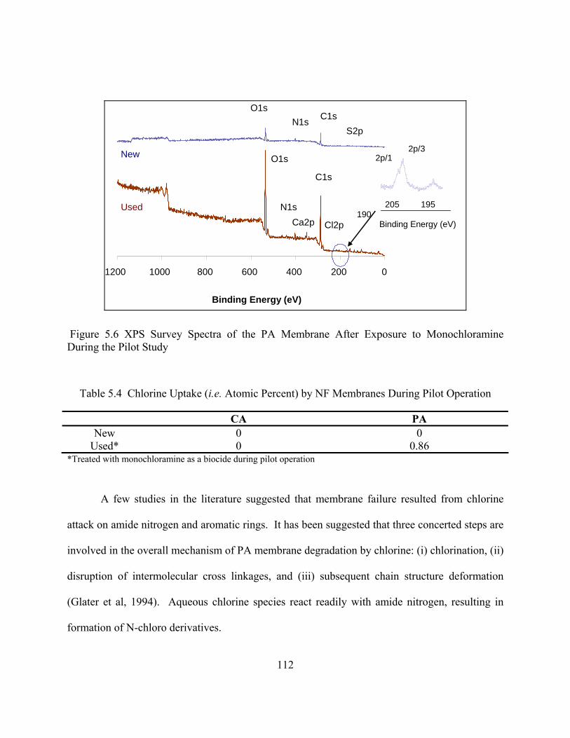
0 200 400 600 800 1000 1200
Binding Energy (eV)
Ca2p Cl2p
O1s N1s C1s
C1s
O1s
N1s Used
New
S2p
2p/12p/3
205 195 190 Binding Energy (eV)
the Pilot Study
Tab
Figure 5.6 XPS Survey Spectra of the PA Membrane After Exposure to Monochloramine During
le 5.4 Chlorine Uptake (i.e. Atomic Percent) by NF Membranes During Pilot Operation
CA PA New 0 0
Used* 0 0.86 *Treated with monochloramine as a biocide during pilot operation
es, and (iii) subsequent chain structure deformation
(Glater et al, 1994). Aqueous chlorine species react readily with amide nitrogen, resulting in
formation of N-chloro derivatives.
A few studies in the literature suggested that membrane failure resulted from chlorine
attack on amide nitrogen and aromatic rings. It has been suggested that three concerted steps are
involved in the overall mechanism of PA membrane degradation by chlorine: (i) chlorination, (ii)
disruption of intermolecular cross linkag
112

Wavenumber (cm-1)
Used
S=O
C=O
C-Cl
Missing C=O
Missing S=O
Figure 5.7 FTIR Scan of the PA Membrane After Exposure to Monochloramine During the Pilot Study
Aromatic rings are also susceptible to electrophilic substitution by chlorine. Ring
chlorination is considered to take place by two possible reaction pathways: direct electrophilic
aromatic substitution and Orton Rearrangement. The second mechanism involves initial
chlorination of amide nitrogen. The resulting N-chloro amide then undergoes intermolecular
rearrangement forming various aromatic substitution products. The exact chemical mechanism
of chlorine-polymer interaction and subsequent membrane failure are not, as yet, clearly
paper by Glater et al. (Glater et al, 1994).
understood. Various possible scenarios for membrane failure were extensively reviewed in a
113

114
Monochloramine Exposure Experiments
In order to verify the impact of monochlo tion on PA membranes observed in the
pilot stu e was statically (i.e. no filtration) exposed to varying doses of
monochloramine (0 to 50 mg/L) for a period of tw s (Beverly, 2000). Th continued
to be used as a primary tool for tracking the uptake of chlorine by membranes. Similar to the
pilot study, chemical degradation of the PA membrane was confirmed by the presence of
chlorine. The chlorine uptake by the membranes increased with increasing monochloramine
dose as shown in Figure 5.8. Tensile strength testing performed on samples exposed to known
doses of monochloramine showed evidence of membrane hardening due to oxidation. This was
evidenced by an increased ability to withstand mechanical loading (Table 5.5). However, the
loss of the ability to stretch under force indicated that the membranes were more brittle after
chlorination. This combination of hardening and loss of ductility would seem to increase the
chance of membrane rupture, particularly under the high pressures used in pilot-scale operation,
explaining PA membrane failure at the presence of monochloramine.
Static
ramina
dy, the PA membran
o week e XPS

0.0
0.5
1.0
1.5
2.5
115
0 5 50
2.0
3.0A
m P
c)
Monochloramine Dose (ppm)
toic
eren
t (%
Figure 5.8 PA Membrane Chlorine Uptake (i.e. atomic percent) by Exposure to Varying Doses of Monochloramine (Bench-Scale Static Evaluation)
Table 5.5 Results of Tensile Strength Tests on PA Membrane
Oxidant/Dose Load at Failure Length at Failure Monochloramine Dose
0 55.0 0.552 5 160.0 0.408
Free Chlorine Dose 5
50 172.5 0.430
165.0 0.328
116
CONCLUSIONS
Control of biogrowth is critical for surface water treatment by NF membrane systems.
The addition of monochloramine was greatly beneficial to prevent biodegradation and associated
its chemical structure. Initially, when operated
rapid decline in water mass transfer coefficient. Monochloramination reduced the rate of fouling
rejection over time. This indicated damage to the membrane and associated integrity issues.
embrane degradation was
The ability of a given membrane to withstand extended exposure to monochloramine
hly investigated to ensure long-term membrane viability, in particular with
monochloramine. It is very important for RO/NF membranes to be chemically compatible with
loss of integrity of the selected cellulose acetate membrane. The selected polyamide membrane
was inherently not biologically degradable due to
without monochloramine feed, the performance of the PA membrane was poor as evidenced by a
but resulted in a gradual increase in water mass transfer coefficient and a decrease in TDS
Based on XPS and FTIR analysis, it was postulated that the PA m
chemically-based and was initiated with chlorination of amide nitrogen and/or aromatic rings,
which ultimately resulted in disruption of membrane chemical structures.
should be thoroug
metal coagulation pretreatment which may further enhance membrane degradation by
monochloramine in order to expand the applications of RO/NF membranes to the treatment of
low quality source waters including surface water and wastewater reclamation, in which
biofouling is expected to be severe.
117
REFERENCES
Alvarez, M., Lozier, J., Johnson, C., Salsano, J., Feb. 2003. “Integrated Membrane Systems: Pilot Test Evaluation for Treatment of Seasonally Brackish Surface Water – Update, AWWA Membrane Technology Conference, Atlanta, GA.
n, 85, 321-334. Avlonitis, S., Hanbury G., and Hodgkiss, T., 1992. Chlorine degradation of aromatic polyamides, Desalinatio
Beamson, G. and Briggs D., 1992. High Resolution XPS of Organic Polymers. New York: John Wiley & Sons.
Bergman, R. A., Sanders, F. A., Fleishcer E. J., Palen G. M., Feb. 1997. “Design Challenges of a Combination Surface Water Plant and Ground Water Desalting Plant at Chesapeake, Virginia”, AWWA Membrane Technology Conference, New Orleans, LA
Beverly S., 2000. Analysis of reverse osmosis and nanofiltration membrane failure by X-ray photoelectron spectroscopy, MS thesis, University of Central Florida
Beverly, S., Seal, S. and Hong, S., 2000. Identification of Surface Chemical Functional Groups Correlated to Failure of Reverse Osmosis Polymeric Membranes, Journal of Vacuum Science and Technology, 18 (4), 1107-1113.
Briggs, D., 1998. Surface Analysis of Polymers by XPS and Static SIMS. Cambridge, UK: University Press.
C. M. Robert, J. S. Taylor, C. R. Reiss, N. Langenderfer, Mar. 1999. “Surface Water Treatment by In-Line Coagulation”, AWWA Membrane Technology Conference, Long Beach, CA.
Connell, G. F., 1997. The chlorination and chloramination handbook, American Water Works Association.
Duranceau S. J., K. A. Thorner, P. D. McAlesse, Nov. 1998. “The Olivenhain Water Storage Project and Integrated Membrane Systems”, Proceedings of Microfiltration II, San Diego, CA
Glater, J., Hong, S., and Elimelich, M., 1994. The search for a chlorine-resistant reverse osmosis membrane, Desalination, 95, 325-345.
118
esalination, 48, 1-16.
e, 132, 159-181.
cal injection points in pretreatment of reverse osmosis (RO) plant performance, Desalination, 167,
Kawaguchi T. and Tamura H., 1984. Chlorine-resistant membrane for reverse osmosis. I. etween chemical structures and chlorine resistance of polyamides, J. Applied
lyme
o J- 1986. ESCA characterization of chlorine damaged lyam
Schippers, Feb. 1997. “Integration of Multi-Objective Membrane Systems For Control of Microbials and DBP-Precursors’, AWWA Membrane Technology Conference, New Orleans, LA
Lowell, J., Friesen, D., McCray, S., McDermott, S., Brose, D., and Ray, R., 1987. Model Compounds as Predictors of Chlorine Sensitivity of Interfacial Polymer RO Membranes. Bend Research, Bend, OR.
Peterson, R., 1993. Composite reverse osmosis and nanofiltration membranes. Journal of Membrane Science, 83, 81-150.
Reiss, R., Taylor J., and Robert. C., 1999. Surface water treatment using nanofiltration: Pilot testing results and design consideration, Desalination, 125, 97-112.
Saeed, M., 2002. Effect of dechlorination point location and residual chlorine on biofouling in a seawater reverse osmosis plant, Desalination, 143, 229-235.
Seal, S., Krezoski, S., Barr, T., and Petering, D., 1997. Journal of Vacuum Science and Technology, A 15(3), May/June, 1235-1245.
Seamans, M., Lozier, J., Kommineni, S., Mar. 2003. “Implications and Issues with Reverse Osmosis Treatment of Air Stripped Groundwater: City of Scottsdale Evaluation”, AWWA Membrane Technology Conference, Atlanta, GA.
Glater J., Zachariah M. R., McCray S. B., and McCutchan J. W., 1983. RO membrane sensitivity to ozone and halogen disinfectants, D
Hong, S., and Elimelich M., 1997. Chemical and Physical Aspects of NOM Fouling of NF Membranes. Journal of Membrane Scienc
Hafsi, M., Khaoua, A., Ben Abdellah, S., and El Mghari Tabib. M., 2004. Effects of the chemi
209-216.
Correlation bPo r Science, 29, 3359-3367.
Ko Y., Petersen R. J. and Cadotte J. E.,po ide reverse osmosis membrane, ACS Polymer Prepr. 27(2) 391-392.
Kruithof, J C, P Hiemstra, P. Kamp, J. van der Hoff, J. Taylor and J.

119
St , D.C.:
Taylor J. and Hong S., 2000. Potable water quality and membrane technology, Journal of Laboratory Medicine, 31 (10), 563-568.
US EPA (1999) Alternative disinfectants and oxidants guidance manual (EPA 815-R-99-014)
VentresSur-Oise Membrane Facility, AWWA Membrane Technology Conference, San Antonio, TX.
2. LFC1, Hydranautics (Oceanside, CA)
4. Memcor CMF, US Filter (Timonium, MD)
andard Methods for the Examination of Water and Wastewater. 19th Ed. (1996) Washington APHA-AWWA-WPCF
que C., Giscion, G., Bablon, G. Chagneau, Mar. 2001, “First Year Operation of he Mery-
FOOTNOTES 1. CALP, Fluid Systems (San Diego, CA)
3. Zeeweed 500, Zenon (Ontario, Canada)
5. Hypersperse 200, Argo Scientific (Minnetonka, MN) 6. 5400 PHI ESCA spectrometer, Physical Electronics (Eden Prarie, MN) 7. Model 575C FTIR spectrometer, Bio-Rad (Cambridge, MA).
120
INTRODUCTION
CHAPTER 6 DIFFUSION CONTROLLED ORGANIC SOLUTE MASS TRANSPORT IN NANOFILTRATION SYSTEMS
al, 1999; Chellam et al, 2001). Mass
transport through diffusion controlled membranes has been investigated (Zhao et al 2005; Taylor
1996). Permeate water quality from RO) and nanofiltration (NF) systems is a
function of solvent and solute tr
nian motion, at a rate dependent on the
differential concentration; and 2) size exclusion, in which solute passage is solely a function of a
pore size (all species smaller than the pore size pass through, all larger species are completely
rejected) (Soltanieh and Gill, 1981; Lee and Lueptow, 2001).
Protocols have been developed (ASTM, 1993: USEPA, 1996) to enhance information
gained from field investigations using membranes, and have been critiqued for suggested
improvements (Zhao et al, 2004). Models have been developed that considered the impact of
time and operating conditions on inorganic mass transfer that shows diffusion control (Mi et al
2003; Lee et al, 2003; Zhao et al, 2005b; Zhao et al, 2004b; Mulford et al, 1999). However, data
on organic compounds are less common and the method of transport is not as clear. This
research investigated Total Organic Carbon (TOC), UV 254, color, Simulated Distribution
Membranes have been shown to be applicable for removal of a wide variety of
contaminants in surface and groundwater (Reiss et
reverse osmosis (
ansport through the membrane film, to the permeate side. Mass
transport theories describe two potential methods of solute transport through a membrane film:
1) diffusion through molecular pores, via Brow

121
ion or size exclusion controlled. A primary goal was
to deter
ontrolled as permeate
concentration would vary with flux and recovery.
Mass Transport
Transport equations for membrane systems have primarily been physical models based
on therm ics and/or statistical m (Weber, 1972). These liquid separation theories
can be placed in three main categories:
• Irrev rsible therm
Solution diffusion theory.
The most common theory used in practice is the solution diffusion theory that describes
solvent and solute flow by Equations (6.1) and (6.2), respectively (Weber, 1972). According to
the solution-diffusion model, each solute is transported by diffusion in response to its chemical
potential gradient. This theory assu embrane surface entirely controlled
onvective flow. Also, it does not account for
coupling effects such as increased calcium rejection in the presence of increased sulfate
System (SDS) Trihalomethane (THM), and SDS Haloacetic Acid (HAA) transport in two NF
systems to determine if passage was diffus
mine if flux and recovery influenced permeate quality to such a degree that water quality
goals and regulatory requirements could only be met within a specific range of flux and
recovery. This would be more likely if mass transport were diffusion c
odynam echanics
e odynamics;
• Preferential sorption capillary flow theory; and
•
mes a semi-permeable m
by diffusion with no porous areas capable of c

122
concentrations. Nevertheless, experimental mass transport results follow solution diffusion
theory and this theory is widely applied.
Equation (6.1) describes the solvent or water flux to be a function of the applied pressure
and the osmotic pressure due to the concentration gradient between the feed and permeate.
Equation 2 describes solute flux as function of the concentration gradient.
( )A
Q∆Π∆PKJ p=−= ww (6.1)
ACQ
∆CKJ ppss == (6.2)
icient, gfd/psi (L/m2/h/bar)
∆P = pressure drop through membrane, psi (bar)
= permeate concentration, mg/L
Where:
Jw = water flux, gfd (L/m2/h)
Kw = water mass transfer coeff
∆Π = osmotic pressure differential through membrane, psi (bar)
Qp = permeate flow, gpd (L/min)
A = surface area, ft2 (m2)
Js = solute flux, mg/ft2-day
Ks = solute mass transfer coefficient, ft/day (m/day)
∆C = concentration gradient through membrane, mg/L
Cp

123
ased on the solution diffusion theory, models have been developed to predict permeate
concentration. (6.3)) incorporates solution diffusion theory and
predicts that permeate concentration would increase with decreasing flux and increasing
recove
B
The linear model (Equation
ry [Taylor, 1996]. The linear model has been used to predict pesticide rejection (Chen et
al, 2004; Duranceau et al, 1992) and operational effects (Reiss et al, 2001) on mass transfer in
diffusion controlled membrane systems.
ss
sfp
Kr2
J
KCC+⎟
⎠⎜⎝ −
=
Where:
2r2 ⎞⎛ − (6.3)
Cf = feed concentration, mg/L
R = water recovery (%/100)
C =
In contrast, for solutes controlled by size exclusion, a simple model as shown in Equation
4 is available (Taylor, 1996) and has been used to model mass transfer in size exclusion
membranes (Robert et al, 2001). Permeate concentration is independent of flux and recovery.
Solutes smaller than the membrane pores can pass through the membrane by convection while
larger constituents can be excluded by size. This model assumes a single distinct molecular
weight cutoff or pore size cutoff and is commonly applied to micro and ultra filtration
membranes.
fp φC (6.4)
124
Nanofiltration membranes are known to have a distribution of molecular pore sizes.
Historical manufacturi patching of larger
imperfections. Therefore, it is possib both conv iffu rt pla n
solute passage. As described above, a change in permeate concentrati ponse g
flux and recovery is descriptive of diffusive transport whereas convective solute transport, based
on equ not vary w lux or re y. This stu assessed pi cale
nanofiltrat ts to determine such ces.
Source Water
s of operation is presented in Table 6.1. As
shown, the total organic carbon (TOC) ranged from 4 to 28 mg/L, total hardness from 50 to 180
Where:
φ = exclusion coefficient
ng techniques have included inspection and
le that ect d dive an sive spo tran y i a role
on res in to in vary
a d tion 4, woul ith changes in f cover dy lot s
ion uni influen
The source water was the Hillsborough River in Tampa, Florida. The Tampa Water
Department owns and operates the David L. Tippen Water Treatment Plant (DLT WTP), a 120
mgd (454 ML/d) conventional ferric coagulation, sedimentation, filtration (CSF) water treatment
plant (WTP) that was the site for this pilot study. The Hillsborough River is a spring fed river
with supplemental supply coming from precipitation and watershed runoff. Water quality varies
greatly between seasons with higher organic levels and lower TDS during the wet season
(summer) and higher TDS and lower organic levels during the dry season (winter).
Water quality observed during 15 month

125
mg/L as CaCO3, and alkalini
surface waters, of this river are higher than mo ces in the United
States.
h Riv lity
Minimum
ty from 30 to 180 mg/L as CaCO3. Though typical of Florida
the TOC levels st other sour
Table 6.1 Hillsboroug er Raw Water Qua
Parameter Units Maximum Average TOC mg/L 27.5 4.0 16.4
UV 254 cm-1 1.9070 0.1508 0.7412 C cu olor 297 34 153
SDS TTHM µg/L 199 224 S g/L 254 683
3 30 0 Total Hardne mg/L as CaCO3 50 8
2,581 1,DS HAA6 µ 3,507 1,Alkalinity mg/L as CaCO
ss 178 184
810
TDS mg/L 270 63 169
METHODS AND MATERIALS
ems were o ted at the DLT W n Tampa,
Florida e acetate (Fluid s CALP) and a polyamide
(Hydranautics LFC1) were evaluated in 2:1 array NF system ents or
two (2) s are shown in Tab .2. River water was reated via
m gpm ilot unit) NF
u 7 and 14 and 24 L/m2/hr) and recoveries
of 65 and 85% for a total of four sets of conditions. Water quality samples were btained for
feed stem.
Pilot Scale Integrated Membrane Syst pera TP i
. Two nanofilters, a cellulos System
s with three (3) 4040 elem
4060 per vessel. Characteristic le 6 pret
icrofiltration (Memcor 0.2 µm pore size, 30 [114 L/min] p and fed to the
n ofits. Each NF system was tested at fluxes gfd (12
o
and both permeate stages of the NF sy
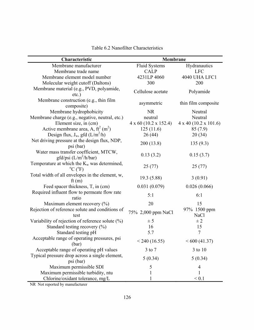
126
Table 6.2 Nanofilter Characteristics
Characteristic Membrane Membrane manufacturer Fluid Systems Hydranautics Membrane trade name CALP LFC
Membrane element model number 4231LP 4060 4040 UHA LFC1 Molecular weight cutoff (Daltons) 300 200
Membrane material (e.g., PVD, polyamide, etc.) Cellulose acetate Polyamide
Membrane construction (e.g., thin film composite) asymmetric thin film composite
Membrane hydrophobicity NR Neutral Membrane charge (e.g., negative, neutral, etc.) neutral Neutral
Element size, in (cm) 4 x 60 (10.2 x 152.4) 4 x 40 (10.2 x 101.6)Active membrane area, A, ft2 (m2) 125 (11.6) 85 (7.9)
Design flux, Jw, gfd (L/m2/h) 26 (44) 20 (34) Net driving pressure at the design flux, NDP,
psi (bar) 200 (13.8) 135 (9.3)
Water mass transfer coefficient, MTCW, gfd/psi (L/m2/h/bar) 0.13 (3.2) 0.15 (3.7)
Temperature at which the Kw was determined, oC (oF) 25 (77) 25 (77)
Total width of all envelopes in the element, w, ft (m) 19.3 (5.88) 3 (0.91)
Feed spacer thickness, T, in (cm) 0.031 (0.079) 0.026 (0.066) Required influent flow to permeate flow rate
ratio 5:1 6:1
Maximum element recovery (%) 20 15 Rejection of reference solute and conditions of
test 75% 2,000 ppm NaCl 97% 1500 ppm NaCl
Variability of rejection of reference solute (%) ± 5 ± 2 Standard testing recovery (%) 16 15
Standard testing pH 5.7 7 Acceptable range of operating pressures, psi
(bar) < 240 (16.55) < 600 (41.37)
Acceptable range of operating pH values 3 to 7 3 to 10 Typical pressure drop across a single element,
psi (bar) 5 (0.34) 5 (0.34)
Maximum permissible SDI 5 4 Maximum permissible turbidity, ntu 1 1
Chlorine/oxidant tolerance, mg/L 1 < 0.1 NR Not reported by manufacturer
128
RESULTS
Average trati rejection, by membrane, are shown in Table 6.3. The
rejection of the CALP membrane was less than that of the LFC1, in all cases. Though water
m co nts ar ar for the emb s (0.13 t fd/psi [ .7
L/m2/h/bar]), the polyamide LFC1 exhibited greater solute rejection. Such enhanced rejection
characteristics of polyamide films over cellulose acetate are well documented and are explained
by differences in surface charge and hydrophobicity [Bitter, 1991; Taylor, 1996; Marinas et al,
1992; Gregor, 1976].
The impact of flux and recovery on permeate TOC concentration is illustrated in Figure
6.1 and Figure 6.2, for the CALP and LFC1 nanofilters, respectively. For the CALP, there is a
clear impact of both flux and recovery on permeate concentrations. The permeate TOC
concentration changed from 1.95 mg/L at worst conditions (flux of 7 gfd [12 L/m2/h] and
recovery of 85%) to 0.50 mg/L at best conditions (flux of 14 gfd [24 L/m2/h] and recovery of
65%). This represents a four fold reduction in permeate concentration as a result of changing the
operational settings. For this membrane, at the feed TOC concentration of 18.8 mg/L,
regulations could be dependent on and controlled by operational settings.
Table 6.3 Average Concentration and Rejection by Nanofilter
con enc on and
ass transfer efficie e simil se two m rane o 0.15 g 3.2 to 3
compliance with United States Environmental Protection Agency disinfection by products
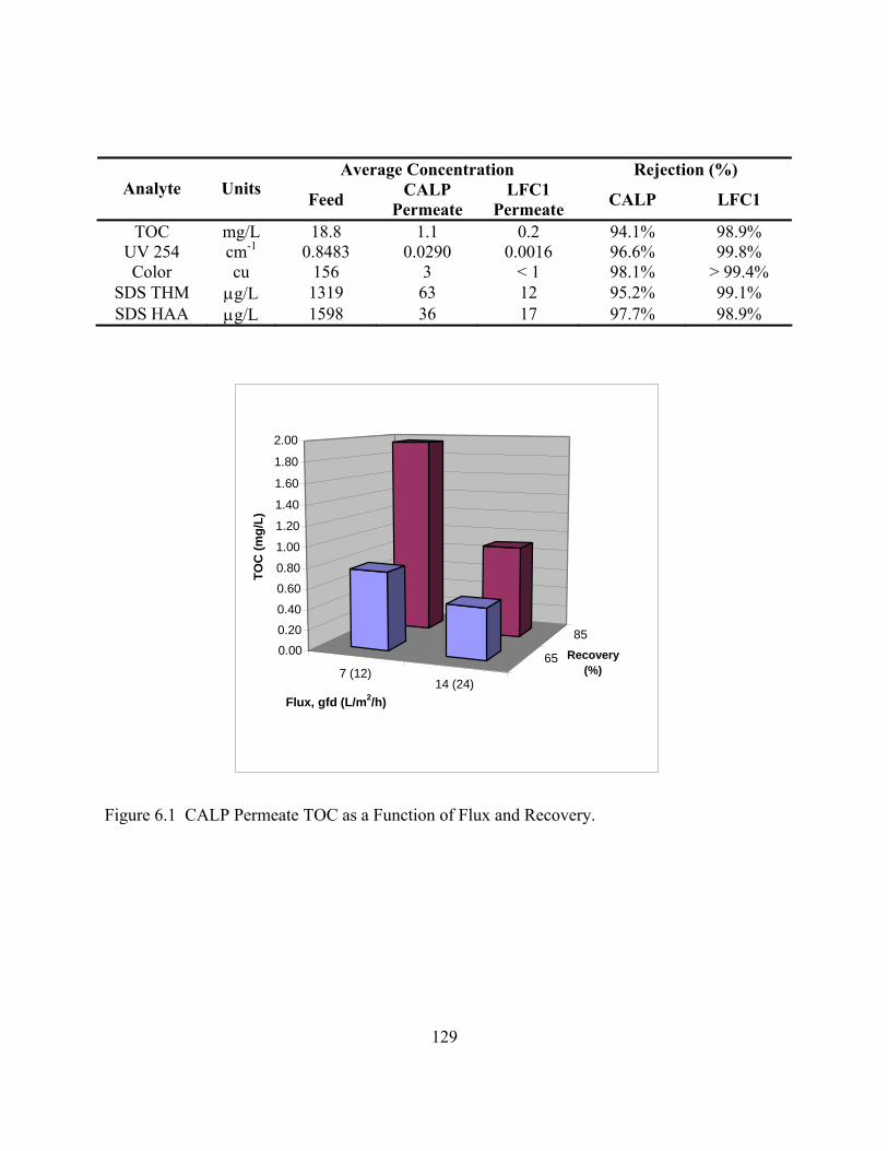
7 (12)14 (24)
65
850.00
0.40
0.80
1.20
1.60
1.80
2.00
TOC
(mg/
L)
Flux, gfd (L/m2/h
Recovery
0.20
0.60
1.00
1.40
)
(%)
Figure 6.1 CALP Permeate TOC as a Function of Flux and Recovery.
Average Concentration Rejection (%) Analyte Units CALP LFC1
TOC mg/L 18.8 1.1 0.2 94.1% 98.9%
Feed Permeate Permeate CALP LFC1
UV 254 cm-1 0.8483 0.0290 0.0016 96.6% 99.8%
SDS THM µg/L 1319 63 12 95.2% 99.1% SDS HAA µg/L 1598 36 17 97.7% 98.9%
Color cu 156 3 < 1 98.1% > 99.4%
129

7 (12)14 (24)
65
850.00
0.10
2
Recovery
0.20
0.50
0.60
TOC
(mg/
L)
0.30
0.40
Flux, gfd (L/m /h)
(%)
Figure 6.2 LFC1 Permeate TOC as a Function of Flux and Recovery.
are
significant enough that regulatory compliance could be a function of flux and recovery for some
sources.
polya anofilter, the influ lux and recove ll
permeate TOC concentrations were less than 0.40 m approac e analytica tion
limit, which is typically 0.1 to 0.5 mg/L for TOC an These res
The variation of permeate TOC with flux and recovery for the CALP NF is consistent
with a diffusion controlled mass transport mechanism defined by Equation (6.3), as evidenced by
the data in Figure 6.1. However, TOC is an aggregate parameter and is composed of organic
molecules that have varying molecular weights and TOC mass transport could be affected by
both size exclusion and diffusion mechanisms. Nevertheless, the effects of diffusion
For the LFC1 mide n e f fnce o ry is diminished. A
g/L and hed th l detec
alysis. ults support size exclusion
130
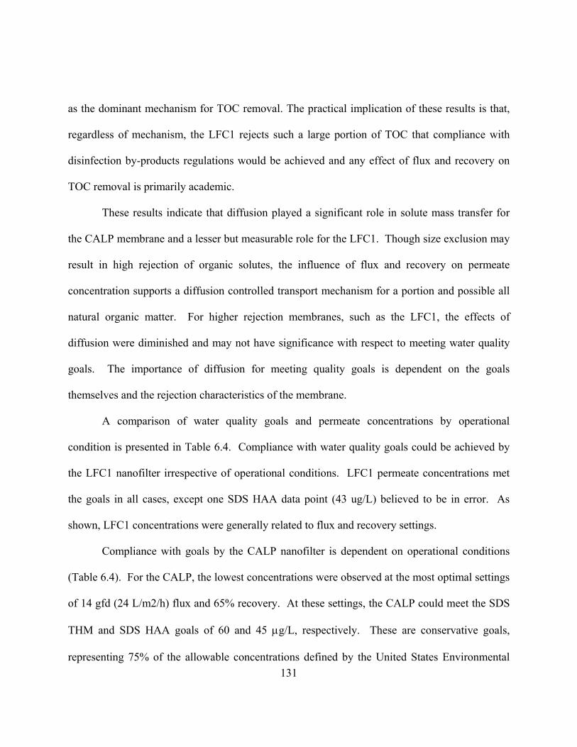
131
a the d chanism TOC rem l. The l implica of these resul that,
regardle echanism, the LFC1 rejects such a large portion of TOC that compliance with
disinfection by-products regulations would be achieved and any effect of flux and recovery on
T C rem arily academic.
ignificant role in solute mass transfer for
the CA
For higher rejection membranes, such as the LFC1, the effects of
diffusio
centrations met
the goals in all cases, except one SDS HAA data point (43 ug/L) believed to be in error. As
shown, LFC1 concentratio settings.
Compliance with goals by the CALP nanofilter is dependent on itions
(Table 6.4). For th the entra ns were t the al settings
of 1 (24 L/ d 65% very. ese s LP c meet the SDS
THM and SDS HAA goals of 60 and 45 µg spec are c rvative s,
representing 75% of the allowable concentrations defined by the United States Environmental
s ominant me for ova practica tion ts is
ss of m
O oval is prim
These results indicate that diffusion played a s
LP membrane and a lesser but measurable role for the LFC1. Though size exclusion may
result in high rejection of organic solutes, the influence of flux and recovery on permeate
concentration supports a diffusion controlled transport mechanism for a portion and possible all
natural organic matter.
n were diminished and may not have significance with respect to meeting water quality
goals. The importance of diffusion for meeting quality goals is dependent on the goals
themselves and the rejection characteristics of the membrane.
A comparison of water quality goals and permeate concentrations by operational
condition is presented in Table 6.4. Compliance with water quality goals could be achieved by
the LFC1 nanofilter irrespective of operational conditions. LFC1 permeate con
ns were generally related to flux and recovery
operational cond
e CALP, lowest conc tio observed a most optim
4 gfd m2/h) flux an reco At th ettings, the CA ould
/L, re tively. These onse goal

132
Protect
Table 6.4 Permeate Concentrations by Operating Condition
Flux/ Recovery TOC Color UV 254 SDS THM SDS HAA
ion Agency (USEPA) Disinfectant/Disinfection Byproducts Rule (D/DBPR) Stage 1
THM and HAA maximum contaminant levels (MCLs) of 80 and 60 µg/L, respectively. More
importantly, this data shows that finished water quality can vary by a factor of 4 or more,
depending on flux and recovery settings. In many applications, this may determine compliance
with water quality goals. Such assessments may be critical to design of membrane systems and
should be conducted at pilot scale for comparison with finished water quality requirements.
gfd (L/m2/h)/% mg/L cu cm-1 µg/L µg/L Goal < 1.0 < 5 < 0.0100 < 60 < 45 Feed 18.8 156 0.8483 1319 1598
CALP 7 (12)/65 0.81 1 0.0162 55 22 7 (12)/85 2.06 7 0.0601 92 69 14 (24)/65 0.57 < 1 0.0128 44 18 14 (24)/85 0.97 4 0.0268 61 35
LFC1 7 (12)/65 0.16 < 1 0.0018 9 12 7 (12)/85 0.37 2 0.0046 19 8 14 (24)/65 0.18 < 1 0.0005 9 43 14 (24)/85 0.13 1 0.0023 10 3
Concentrations are flow weighted averages of Stage 1 and Stage 2 permeate concentrations. Bold indicates lowest concentration observed.
The linear homogeneous solution diffusion model was utilized to quantify the impact of
tion diffusion model
was solved for KS, the solute mass transfer coefficient. Four data points were available for each
analyte, by m
flux and recovery on permeate concentration. The linear homogenous solu
embrane.

133
hown by higher solute mass transfer coefficients.
Table 6.5 Solute Mass Transfer Coefficients
CALP LFC1
Regression coefficients for all solute/membrane combinations converged in during
regression except for the LFC1-SDS HAAs pair as shown in Table 6.5. These results indicate
diffusion control for organic mass transfer through both membranes excepting the LFCI-SDS
HAA combination. The diffusion effect is also supported by the relative high R2 values on Table
6.5. Note that in all cases, the influence of flux and recovery on solute transport was higher for
the CALP than the LFC1, as s
Parameter Ks, gfd (L/m2/h) Converged R2 Ks, (gfd)
(L/m2/h) Converged R2
TOC 0.208 (0.048) Yes 0.95 0.035 (0.059) Yes 0.68 Color 0.075 (0.127) Yes 0.74 0.024 (.0407) Yes 0.68
UV254 SDS-THM 0.15 (0.255) Yes 0.64 0.028 (0.0475) Yes 0.75 SDS-HAA
0.122 (0.207) Yes 0.87 0.009 (.0153) Yes 0.93
0.076 (0.129) Yes 0.87 0.019 (0.0323) No NA
The linear homogeneous solution diffusion equation accurately predicted TOC mass
transfer through either membrane for the conditions of this work. As shown in Figure 6.3, TOC
has limited variability, indicating diffusive transport was significant, with respect to TOC
passage. These results are significant in that organic solute mass transport through nanofiltration
systems appears to follow solution diffusion theory with the linear homogeneous solution
diffusion model providing reasonable representation of the effects of flux and recovery on
permeate concentration.
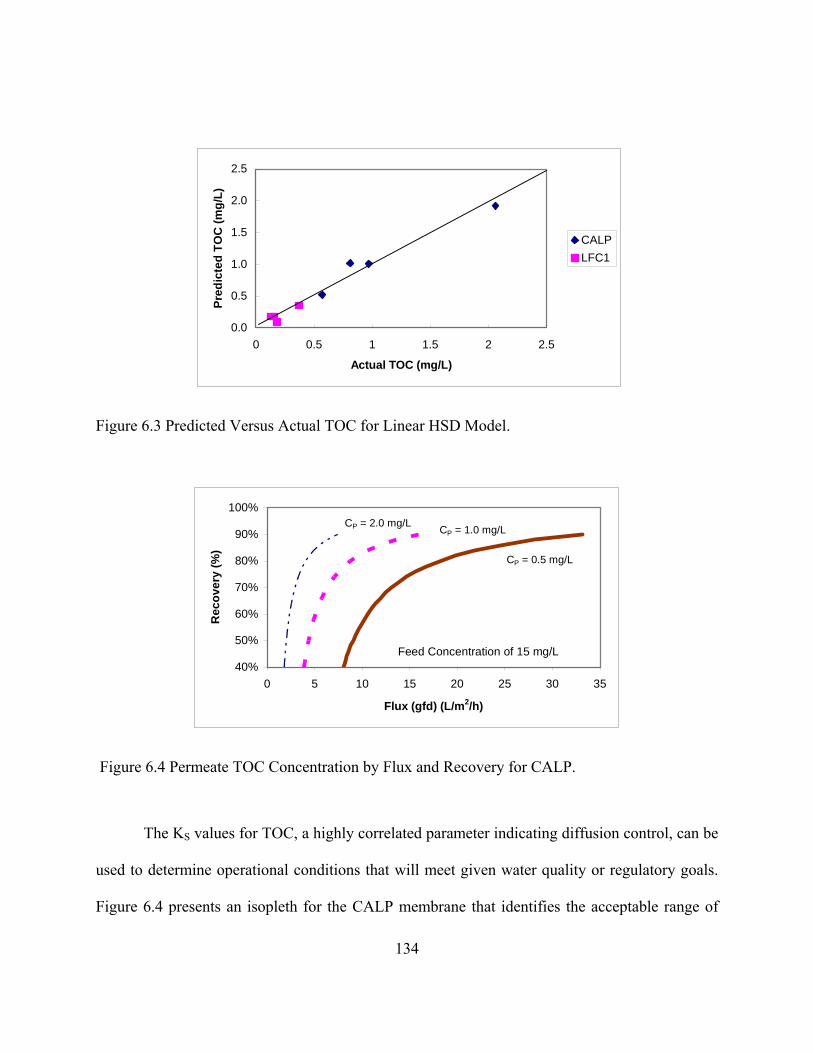
0.0
0.5
1.0
1.5
2.0
0 0.5 1 1.5
Pred
cted
TO
C (m
/L)
2.5
2 2.5
ig
CALPLFC1
Actual TOC (mg/L)
redicted Versus Actual TOC for Linear HSD Model. Figure 6.3 P
40%
50%
60%
70%
80%
90%
Rec
ove
(%)
100%
0 5 10 15 20 25 30 35
Flux (gfd) (L/m2/h)
ry
CP = 0.5 mg/L
CP = 2.0 mg/L CP = 1.0 mg/L
Feed Concentration of 15 mg/L
Figure 6.4 Permeate TOC Concentration by Flux and Recovery for CALP.
The KS values for TOC, a highly correlated parameter indicating diffusion control, can be
used to determine operational conditions that will meet given water quality or regulatory goals.
Figure 6.4 presents an isopleth for the CALP membrane that identifies the acceptable range of
134

135
flux and recovery, to meet a given perm For a goal of TOC < 0.5 mg/L and a
typical recovery of 85%, the system would need to operate at a flux of at least 24 gfd (41
As this illustrates,
on previously collected data.
CONCLUSIONS
eate TOC goal.
L/m2/h), which could increase the rate of fouling and may not be sustainable.
this model provides an effective method of identifying acceptable operational conditions based
• For a size-exclusion controlled membrane, with a pore size distribution and solutes
to not vary with increasing flux or recovery. For a diffusion controlled membrane,
tion increases with recovery and decreases with flux.
greater for a polyamide (PA) than a cellulose acetate (CA) membrane. The PA
rough the membrane were
with decreasing flux for both the PA and CA membranes. The influence was
• Finished water quality, for both the PA and CA NF, is a function of operational
d decreasing
that fall within the distribution size range, permeate concentration would be expected
permeate concentra
• For nanofilters of comparable productivity, rejection of organic-related analytes was
membrane rejected 99% of TOC compared to 94% for the CA nanofilter.
• A significant portion of the organic solutes passing th
diffusion controlled. Permeate concentration increased with increasing recovery and
diminished for the PA membrane, due to its high rejection capabilities.
settings (flux and recovery). The combined effect of increasing flux an
136
TOC and other organic parameters. Consideration should be given to this effect in
A membrane, SDS THM
14 gfd [24 L/m2/h]) and lower recovery (< 65%).
ion model allowed interpretation of expected
and feed water quality.
recovery resulted in as much as a four fold reduction in permeate concentrations of
design of any membrane system. Pilot testing should evaluate this effect for
comparison with finished water quality goals.
• For the PA membrane rejection was high enough that water quality goals were met
irrespective of the influence of flux and recovery. For the C
and SDS HAA goals of 60 and 45 ug/L, respectively, could be met at higher flux (>
• The linear homogeneous solution diffus
finished water quality for various organic solutes at varying flux and recovery settings
137
REFERENCES
ASTM 1993 The Annual Book of ASTM Standard, Designation: D 4516-85.
Bitter, J.G.A., 1991. Transport Mechanisms in Membrane Separation Processes. Plenum Press, New York.
Chellam
Chen S-S, J. S. Taylor , L. A. Mulford and C. D. Norris, Jan. 2004. "Influences of molecular
membranes", Desalination, Volume 160, Issue 2, 15, 103-111.
Duranceau, S. J., Taylor, J. S., 1992. A SOC Removal in a Membrane Softening Process, Jour. of
Lee, J., Taylor, J.S., and Hong, S.K., 2003. “Resistance and Diffusion Modeling for RO and NF
Membrane Technology Conference, Atlanta, Georgia.
Mulford, L.A., Taylor, J.S., Nickerson, D., and Chen, S.S., 1999. Comparison of Full- and Pilot- Scale Nanofiltration on Plant Performance”, Journal AWWA vol. 91, No. 6, 64-75.
, S. and Taylor, J. S., 2001. "Simplified Analysis of Contaminant Rejection During Ground-and Surface Water Nanofiltration Under the Information Collection Rule." Wat. Res. 35(10): 2460-2474
weight, molecular size, flux, and recovery for aromatic pesticide removal by nanofiltration
AWWA, 84:1:68.
Gregor, H.P., 1976. Fixed Charge Ultrafiltration Membranes, in Charge Gels and Membranes, Part 1, ed. E. Selegny, 57-69.
Lee, S. and Lueptow, R.M., 2001. Membrane Rejection of Nitrogen Compounds, Environ. Sci. Technol. 35: 3008-3018.
Productivity and Water Quality”, Proceedings of the American Waterworks Association
Marinas, B. and Selleck, R.E., 1992. “Reverse Osmosis Treatment of Multicomponent Electrolyte Solutions, J. Membrane Science, 72, 211-229.
Mi, B., Rose, J., and Marinas, B.J., 2003. “Investigating the Role of Pore Size Distribution in the Passage of Microorganisms and Solutes Through Nanofiltration Membranes” Proceedings of the American Waterworks Association Membrane Technology Conference, Atlanta, Georgia.

138
Reiss, Nanofiltration –Pilot Testing”, Desalination vol. 125 97-112.
Models. Chem. Eng. Commun. 12: p 279-363.
Taylor, J.S., 1996. Reverse Osmosis and Nanofiltration, in Water Treatment Membrane
cesses for Water Quality Control, John Wiley and Sons, New York, NY.
Zhao Yu and J. S. Taylor, 2005. "Incorporation of Osmotic Pressure in an Integrated Incremental
159.
the Modified Solution Diffusion Model and Artificial Neural Networks", Journal of Membrane
C.R., Taylor, J.S., and Robert, C.M., 1999. “Surface Water Treatment Using
Reiss C. R., J. S. Taylor, C. Robert, and S. Hong, Mar. 2001, "Cumulative Mass-Based Modeling of Nanofiltration Productivity" Proceedings of American Water Works Association (AWWA) 2001 Membrane Technology Conference, , San Antonio, Texas.
Robert, C., J. S. Taylor and C. R. Reiss, 2001. "Resistance Modeling of Size Exclusion Productivity", Proceedings of American Water Works Association (AWWA) Membrane Technology Conference, March 4 - 7, 2001, San Antonio, Texas.
Soltanieh, M. and Gill, W.N., 1981. Review of Reverse Osmosis Membranes and Transport
Processes, ed. P. Jacobs, et al., McGraw-Hill, NY.
USEPA, April 1996. "ICR Manual For Bench and Pilot Scale Treatment Studies", EPA 814-E-96-003.
Weber, W.J. Jr., 1972. Physicochemical Pro
Model for Predicting RO or NF Permeate Concentration", Desalination, vol. 174 no. 2 pp. 145-
Zhao Yu and J. S. Taylor, Dec. 2004b. "Modeling Membrane Performance over Time, JAWWA, 96:12.
Zhao Yu and Taylor, J. S., In Press, Nov. 2004. "Assessment of ASTM D 4516 for Evaluation of Reverse Osmosis Membrane Performance ", Desalination No. 2958.
Zhao Yu and Taylor, J. S., In Press, May. 2005b. "Predicting RO/NF Solute Mass Transfer by
Science.

139
INTRODUCTION
CHAPTER 7 REJECTION OF MICROBIAL CONTAMINANTS BY MEMBRANE SYSTEMS
particularly at risk. The Food and Drug
Administration have accepted no
Inadequate and compromised drinking water supplies are a worldwide public heath
concern. Over 100 different pathogenic waterborne organisms including protozoa, bacteria and
viruses have been identified in contaminated drinking water. Cryptosporidium and Giardia are
waterborne protozoa that have been found in some municipal water systems supplied by surface
water or groundwater under the influence of surface water (Fox and Lytle, 1996). These
parasites, which are not species specific, are excreted in a fully infective form by an infected
human or animal. Infection by Cryptosporidium or Giardia is characterized by severe diarrhea
and nausea. Immuno compromised individuals are
therapies for cryptosporidiosis, although some therapies have
achieved limited success for giardiasis. Cryptosporidium is a significant cause of waterborne
disease in the United States, based on documented contamination of Cryptosporidium in drinking
water, which has also occurred in the United Kingdom, Japan and Holland. The largest U.S.
outbreak occurred in Milwaukee, WI in 1993, where an estimated 450,000 people became ill and
144 died due to contamination of the water supply (Hoxie et al. 1997). The average number of
samples testing positive for Cryptosporidium in groundwater have ranged from 9.5 to 22 percent
Hancock (1998).
140
is, Norwalk, rotavirus and coxsackie viruses.
Gerba
Interim Enhanced
SWTR
ed States and worldwide. Hence, the removal of
Virus contamination in groundwater is of particular concern because of their sub micron
size and transport through soil structures. Illnesses most commonly associated with viral
contamination include, but are not limited to, hepatit
and Rose (1989) reported viruses can survive several months in groundwater.
LeChevallier (1996) reported viral contamination in approximately 20 to 30 percent of
groundwater systems did not correlate with coliform contamination. Coliform, heterotrophic
plate count, chlorine level and Mycobacterium avium complex (MAC) were not correlated in
samples taken from drinking water reservoirs in a study (Glover, 1994). MAC is particularly
invasive in immunocompromised conditions, which are common to individuals with AIDS,
neoplastic disorders or post-heart transplant (Novick, 1990). Cholera, Helicobacter pylori and E.
Coli O157:H7 are additional bacterial agents responsible for waterborne disease, which have had
historically devastating effects worldwide.
In the United Statues, current and proposed regulations require that water treatment
systems meet specific microbial removal efficiencies. The United Statues Environmental
Protection Agency (USEPA) Surface Water Treatment Rule (SWTR) and
are intended to protect against the adverse health effects of Giardia, Legionella,
Cryptosporidium and viruses. The United States Environmental Protection Agency currently
requires at least 4-log removal/inactivation of Giardia and has proposed that potable water
treatment systems using surface water sources provide as much as six-log removal/inactivation
of Cryptosporidium (Alspach and Allgeier, 2005). In addition, control of E. coli, and other
pathogens remains a key focus in the Unit
141
known
ses
includi
embranes have been selected for use in part because of their ability to removal many
differen
aged elements and greater than four-log rejection for
and unknown pathogens is highly desirable in drinking water treatment. More effective
pathogens barriers are needed for incidental and intentional microbial contaminant protection.
Membrane treatment systems have the potential to provide significant single barriers and
even greater cumulative barriers to microbial contaminants including Cryptosporidium
(Askenaizer, Sakaji, and Jacangelo, 2005). Size-exclusion-controlled processes including
microfiltration and ultrafiltration are finding increased applications in the potable water market
to remove turbidity, pathogens and other contaminants. Diffusion-controlled filtration proces
ng nanofiltration and reverse osmosis are primarily utilized for removal of inorganic ions
but have the ability to reject pathogenic microorganisms. Integration of multiple treatment
technologies that utilize at least one membrane unit process, denoted Integrated Membrane
System (IMS), have significant potential to meet drinking water microbial removal requirements
as a multiple barrier to contaminants.
M
t microorganisms, yet surprisingly little information has been documented to
quantitatively state the microorganism removal capacity of membranes (Urban and Manhem,
1997). Membrane pilot studies have demonstrated complete or very high microorganism
removal but few have used microorganism challenge studies to demonstrate the microorganism
removal capacity of membranes (McNamara and Gavin, 1997, Mourato, Newcombe and Leslie,
1997). Visual inspection and dye testing, vacuum testing, E-Coli tracer studies and particle
counting have been compared for assessment of membrane integrity on a field scale. E-Coli
tracer studies were superior to other techniques for assessing integrity because of their ability to
show less than one log rejection in dam
142
intact e
ection for MS2 phage and
aerobic spores, but found only five-log rejection for Cryptosporidium parvum oocysts in MF
field studies. The difference in sample collection volumes
and organism feed stream concentrations. Similar results have been found in a laboratory study.
Colvin et al. (1999) found greater than seven log rejection of MS2 phage in flat sheet studies of
RO membrane films and lack of correlation of microsphere and organism rejection. In a later
publication on the field study, Colvin
sion-controlled mechanism and that membrane
system
lements. In this same study, greater than five to six log removal was demonstrated for
Cryptosporidium parvum oocysts and Giardia Muris cysts. Greater than four log removal was
demonstrated for MS2 phage (Seyde et al., 1999).
Hong et al. (1999), demonstrated greater than six-log rej
organism rejection was attributed to
et al. (2001) found that pressure decay testing, particle and
turbidity monitoring of damaged and undamaged membranes could detect fiber failure of UF or
MF membranes and demonstrated repair of damaged membranes returned performance to that at
the undamaged state. Kruithof et al. (2001) in a large scale pilot study in the Netherlands found
that undamaged UF membranes removed greater than 5.4 log of MS2 phage and that vacuum
testing successfully identified damaged membranes from the manufacturers.
Studies of pathogen removal and integrity of membrane systems show pathogens are
removed by a size exclusion as opposed to a diffu
s reliably reject two to six logs more pathogens than conventional water treatment systems
(Jacangelo et al, 1995, Kriuthof et al, 2001; Lovins et al, 2002). Organism size did not correlate
to log rejection for virus, bacteria or cyst rejection by nanofiltration or ultrafiltration, but did
correlate to log rejection for microfiltration.

143
State regulatory have been recently
documented (Allegier, 2001). As o 29 states F enty-one states
awarded 2 to 3-log credit for Gi Only six arded o-log r
Crypto t has been re equired by terim En ed Surfa ter
Treatme e majority nt any for virus inaction to either MF or
UF. No such assessment has been nofiltration or reverse osm , which highlights
the need for studies on and regulatory recognition of membrane rejection of microorganisms.
Large-scale testing of Cryptosp tion capabilities of various treatment
technologies can be econom
Adham et al, 1998, Seyde et al, 1999). As described previously, pathogen evaluations of
membrane systems while treating natural source waters provides a conservative measure of
expected pathogen removal capabilities.
issues facing ultrafiltration and microfiltration
f 2001, had UF or M plants. Tw
ardia. states aw the tw credit fo
sporidium tha cently r the In hanc ce Wa
nt Rule. Th of states do not gra credit
made for na osis
oridium rejec
ically prohibitive and can involve health risks. Therefore, this work
describes the rejection of aerobic spores (Bacillus subtilis endospores) by several membranes
systems as a surrogate for Cryptosporidium. It has been shown that Bacillus subtilis bacterial
endospores can be used as surrogates for the protozoans Cryptosporidium and Giardia (Rice,
1994).
Reported pore sizes and molecular weight cutoffs for membrane systems are 1 – 3 log
orders smaller than pathogenic bacteria and protozoa’s of concern in potable water supplies. As
such, membranes are expected to provide significant removal of such microorganisms.
However, imperfections in manufacturing and the inherent distribution of pore sizes for all
separation processes can result in less than complete removal. Studies have shown that rejection
of microorganisms is not absolute in membrane systems (Taylor et al, 1998, Reiss et al, 1999,

144
To document the removal efficacy of membrane systems, pilot scale testing was
performed using a s. These
treatment e challenged with c Bacillus sub pores, w e a
docum gate, and removal capabilities measured.
METHODS AND MATERIALS
Florida, USA surface water and various membrane treatment system
systems wer ultured tilis endos hich ar
ented protozoa surro
Source Water
The source water for this research was the Hillsborough River in eastern Hillsborough
County, Florida. The Tampa Water Department owns and operates the David L. Tippen Water
Treatment Plant (DLT WTP), a 120 mgd (454 ML/d) conventional ferric coagulation,
sedimentation, filtration (CSF) water treatment plant (WTP) that was the site for this pilot study
project. The Hillsborough River is a spring-fed river with supplemental supply coming from
precipitation and watershed runoff. Water quality varies greatly between seasons with higher
organic levels and lower TDS during the wet (summer) season and higher TDS and lower
.
Water quality observed during 15 months of operation is presented in Table 7.1. As
shown, the total organic carbon (TOC) ranged from 4 to 28 mg/L, total hardness from 50 to 180
to 180 mg/L as CaCO3. Though typical of Florida
surface waters, the TOC levels of this river are higher than most other sources in the United
States.
organic levels during the dry (winter) season
mg/L as CaCO3, and alkalinity from 30
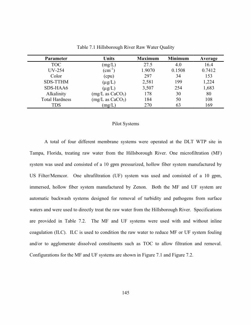
145
Table 7.1 Hillsborough River Raw Water Quality
Parameter Units Maximum Minimum Average TOC (mg/L) 27.5 4.0 16.4
UV-254 (cm-1) 1.9070 0.1508 0.7412
SDS-TTHM (µg/L) 2,581 199 1,224
Alkalinity (mg/L as CaCO
Color (cpu) 297 34 153
SDS-HAA6 (µg/L) 3,507 254 1,683 3) 178 30 80
Total Hardness (mg/L as CaCO3) 184 50 108 TDS (mg/L) 270 63 169
Pilot Systems
A total of four different membrane systems were operated at the DLT WTP site in
Tampa, Florida, treating raw water from the Hillsborough River. One microfiltration (MF)
system was used and consisted of a 10 gpm
are
automa
pressurized, hollow fiber system manufactured by
US Filter/Memcor. One ultrafiltration (UF) system was used and consisted of a 10 gpm,
immersed, hollow fiber system manufactured by Zenon. Both the MF and UF system
tic backwash systems designed for removal of turbidity and pathogens from surface
waters and were used to directly treat the raw water from the Hillsborough River. Specifications
are provided in Table 7.2. The MF and UF systems were used with and without inline
coagulation (ILC). ILC is used to condition the raw water to reduce MF or UF system fouling
and/or to agglomerate dissolved constituents such as TOC to allow filtration and removal.
Configurations for the MF and UF systems are shown in Figure 7.1 and Figure 7.2.

146
Table tration and Ultrafiltration Spec s
Paramet Units
7.2 Microfil ification
er Memcor Zenon Model CSF Z W500
Pore siz ns 0Fiber configuration
M Pressurized
e (nominal) Micro .2 0.05
odule configuration Hollow Hollow
Immersed
Raw Water
Feed Pump
Filtrate
Filtrate
Pressure Vessel
Hollow Fiber
Figure 7.1 Memcor MF Pilot Configuration

Filtrate Tank
Raw Water
Vacuum Pump
Hollow Fiber
Raw Water Tank
Figure 7.2 Zenon UF Pilot Configuration
Two nanofiltration (NF) systems were utilized to treat filtrate from either the MF or the
UF system. MF and UF systems remove contaminants from water by size-exclusion as the
contaminants removed are just too large to pass through the UF or MF membrane. All dissolved
constituents pass through the system and into the filtrate. Nanofiltration has been shown to be
particularly effective in removing TOC, disinfection by-products precursors, taste and odor
compounds, and other dissolved constituents from surface and ground waters (Taylor et al.,
1992; Reiss and Taylor, 1991 for low turbidity (0.2 NTU)
feed waters and will foul by plugging of particulates into the NF pores if used directly on surface
water supp
). However, NF systems are designed
lies (Reiss and Taylor, 1995). Therefore, use of NF systems for surface water
applications requires pretreatment such as MF or UF.
147

148
tal pressure vessels (Figure 7.3). Each element is typically 40” or 60” in length
with ap
While NF systems require low turbidity feed water to avoid plugging, they do remove
particles and pathogens. Use of an NF system downstream of MF or UF treatment constitutes a
multiple barrier approach for pathogen removal and was evaluated as part of this research.
The configuration of NF systems has been standardized and is accepted worldwide.
Commercial configurations consist of either 4” diameter or 8” diameter membrane elements
housed in horizon
proximately 240” to 280” of membrane length per pressure vessel). Spiral wound NF
elements are provided by a number of manufacturers. The two spiral wound NF elements tested
in this project were the Hydranautics LFC1 and the Fluid Systems CALP. Specifications for
each NF element are provided in Table 7.3. The configuration of the pilot-scale NF systems
used to house the LFC1 and CALP membranes is shown in Figure 7.3.
Table 7.3 Nanofiltration Specifications
Parameter CALP LFC1 Manufacturer Fluid Systems Hydranautics
Element configuration Spiral wound Spiral wound
Molecular weight cutoff (Daltons) 200 300
Membrane material (e.g., PVD, polyamide, etc.) acetate polyamide
Membrane construction (e.g., thin-film composite) asymmetric composite
Active membrane area of membrane element used, A (ft
Membrane trade name CALP LFC
cellulose
thin-film
Element size (e.g., 2.5" x 40", 4" x 40", etc.) 4' x 60" 4' x 40"
Water mass transfer coefficient, MTCW (gfd/psi) 0.13 0.15 aximum permissible SDI 5 4
Acceptable range of operating pressures <240 psi < 600 psi
2) 125 85
M
Acceptable range of operating pH values 3 to 7 3-10
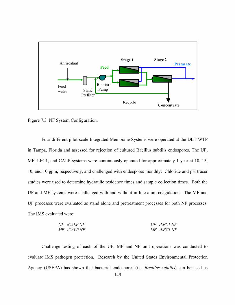
Booster Pump
Permeate
Concentrate
Feed water
Feed
Static
149
Prefilter
Stage 1 Stage 2 Antiscalant
Recycle
Figure 7.3 NF System Configuration.
Four different pilot-scale Integrated Membrane Systems were operated at the DLT WTP
in Tampa, Florida and assessed for rejection of
MF, LFC1, and CALP systems were continuously operated for approximately 1 year at 10, 15,
10, and
MF→CALP NF MF→LFC1 NF
cultured Bacillus subtilis endospores. The UF,
10 gpm, respectively, and challenged with endospores monthly. Chloride and pH tracer
studies were used to determine hydraulic residence times and sample collection times. Both the
UF and MF systems were challenged with and without in-line alum coagulation. The MF and
UF processes were evaluated as stand alone and pretreatment processes for both NF processes.
The IMS evaluated were:
UF→CALP NF UF→LFC1 NF
Challenge testing of each of the UF, MF and NF unit operations was conducted to
evaluate IMS pathogen protection. Research by the United States Environmental Protection
Agency (USEPA) has shown that bacterial endospores (i.e. Bacillus subtilis) can be used as

150
surface waters. The spores are ellipsoidal to spherical
in shap
Bacillus subtilis endospores were cultured by City of Tampa Laboratory staff. Endospore
culturing and enumeration techniques followed methods described for the milk industry for the
detection of sulfa drugs and antibiotics in milk and used in the pharmaceutical industry for the
assay of heat resistant microbial endospores. Samples were heat shocked and assayed for
bacteria by filtration on nutrient agar with trypan blue. Though indigenous to soils and water,
the concentration of naturally occurring aerobic sporulating bacteria present in the Hillsborough
River, Florida is variable. A concentration of endospores that could demonstrate a five to six log
reduction necessitated inoculating each membrane process train with an endospore suspension of
Bacillus subtilis.
Bacillus subtilis ATCC 6051 was rehydrated in Tryptic Soy Broth (TSB) (Difco 0370-17-
3) and transferred to TSB in test tubes and Nutrient Agar (BBL 12447) slants. All culturing of B.
subtilis was at 35oC for 16-20 hours. Healthy growth was streaked on nutrient agar for isolation.
Isolates were gram-stained and spore-stained with malachite green (Sigma) to confirm
surrogates for the protozoas Cryptosporidium and Giardia (Rice, 1994). These organisms
propagate in the soil and are ubiquitous in
e and on average measure approximately 0.5 x 1.0 x 2.0 µm. The membrane unit
processes were challenged with approximately 1 x 10⁷ cfu/100 ml of Bacillus subtilis cultured
on-site by the Tampa Water Department laboratory. The log rejection of spores for each unit
process was summed by IMS, to provide an estimate of the expected IMS performance.
Bacillus subtilis Culturing Procedure

151
morphology by microscopy. Culture maintenance was performed by placing an isolate on slants
of nutrient agar with 0.01% trypan blue.
An extract of African Violet Soil (local nursery) was prepared by making a 38.5%
solution of soil, 0.1% Na2CO3, in deionized water and sterilizing for one hour. Just prior to use
the extract was filtered through 11cm Whatman 40 filter paper. A sporulation agar was prepared
by making nutrient agar with 25% filtered extract of African Violet Soil. This sporulation agar is
less expensive to produce than commercially available products. Sporulation agar was sterilized
in glass milk dilution bottles (Kimax) and laid down to solidify. Growth from a 24h culture on
nutrient agar slant was suspended in 0.85% saline and 0.5 to 1 mL placed on sporulation agar for
four days at 35oC.
Healthy growth on sporulation agar was harvested in sterile 0.85% saline. The harvested
suspension was centrifuged (3000xg) and the pellet was made 0.85% saline, 0.1% (w/v) Tween
to prevent cells from aggregating. Heat shocks were performed in a shaking water bath
(Precision Model 50) by heating to 80°C for 12 minutes in glass bottles, followed by
immediately cooling in an ice bath. A dilution series in 0.85% saline was filtered on 47mm
diameter, 0.45µm pore size filter (Gelman, GN-6) and the filter placed on nutrient agar with
trypan blue in 9 x 50mm plates (Gelman). Colony forming units (cfu) are countable after 16-20
be stored several months at 4°C. However, a fresh
suspension was prepared for each monthly protocol. Yields for this procedure approximate 4.5 x
108 cel
hours at 35°C. The suspension can
ls per cm2 or 1010 cfu/mL with a volume of about 50mL. A heat shock of Escherichia coli
ATCC 11775 produced a four to five log reduction of a suspension in sterile buffered water.
152
The removal efficacy of the membrane pilot plants was evaluated by challenging the
treatment systems with concentrations of endospores of at least 107 cfu/100 ml in the seeded feed
water and measuring the resulting concentration in the permeate streams. The pilot units were in
continu
0 mL in the seeded feed water (Figure
7.4).
ions used to inoculate the process trains were heat shocked and assayed at the same
time. This provided actual concentrations in and out of the pilot system for determining log
emoval rates.
Bacillus subtilis Challenge Testing and Sampling Procedure
ous operation at normal operational settings throughout the course of the challenge
testing. Inoculation of feed water for each membrane process train was based on the volume of
raw or pretreated water presented to the train and the concentration of endospores in the prepared
suspension. The prepared suspension was injected into the feed stream at a rate as was
theoretically required to obtain approximately 107 cfu/10
For the NF challenge tests, endospores were injected downstream of the MF or UF
pretreatment system and upstream of the NF pressure vessels. The NF cartridge filters were
removed for the period of challenge testing, to provide a conservative measure of the removal
capability of the NF elements themselves.
Seeded feed water was sampled to obtain the inoculum for the train. Permeate samples
before and after inoculation are obtained with two time points obtained after inoculation.
Samples collected from sample points were heat shocked and diluted in sterile 0.85% saline if
necessary to produce 10 to 300 cfu by membrane filtration on nutrient agar with trypan blue.
The suspens
r
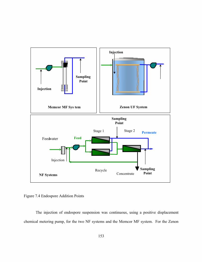
153
The injection of endospore suspension was continuous, using a positive displacement
chemical metering pump, for the two NF systems and the Memcor MF system. For the Zenon
Figure 7.4 Endospore Addition Points
Permeate Feed water Feed
Stage 1 Stage 2
Recycle
Inje ction
Sampling Point
Sampling Point
Memcor MF Sys tem Zenon UF System
Injection
Injection
Sampling Point NF Systems Concentrate

154
UF sys
jected
endospore suspension had adequate tim
eas spore concentration from the two-stage NF unit following
spiking of the NF feed stream can be described as a second order model where n is two for each
NF stage.
tem, the necessary aliquot of suspension was added to the reactor tank and mixed using
the diffused air system.
Tracer Studies
The injection of endospore suspension was continuous using a positive displacement
chemical metering pump, for the MF and NF systems, and was batch for the UF system. Tracer
studies were performed on each of the four membrane pilot units to ensure that the in
e to travel through the treatment unit and be captured in
the subsequent filtrate sample collected from each unit.
Hydraulic residence times (HRTs) of all membrane units must be known to determine the
sampling times for challenge studies. HRTs in membrane systems have been described by a
complete mix model as shown in Equation (7.1), which is integrated with respect to time as
shown in Equation (7.2) (Duranceau, 1991). Effluent stream concentration from any number of
unit operations in series for only mixing can be determined from the expanded model as shown
in Equation (7.3). Practically, filtrate stream concentration following can be described as a first
order model where n is one; wher
spike-ospike-t kC-
dtdC
= (7.1)
(7.2)
kt-spike-ospike-t eCC =

( )-
-
×-
××= tτnt1n
spike-ospike-t e!1n
1τnt
nCC (7.3)
Where:
o-spike = time zero
t-spike = time since initiation of spike
NaCl was used as a tracer to determine the HRT of the UF unit. NaOH was used to
adjust pH, which served as a tracer to determine the HRT of the MF. Sulfuric acid was used as a
nvenience and necessity as NaCl is significantly rejected by NF.
Chloride and pH adjustments were made in the UF and MF/NF units respectively and monitoring
of the UF/MF and NF effluent as initiated. The NF permeate
stream pH is shown in Figure 7.5. Exponential second-order behavior of declining pH of the NF
permeate stream is eviden
onservative sampling times of 2 and 4 minutes were established for collection of
samples following initiation of endospore suspension introduction.
tracer for the NF units for co
streams for HRT determination w
t in Figure 7.5.
As noted, the UF hydraulic residence time was determined from a chloride tracer study.
Sodium chloride was added to the UF tank and mixed through operation of the diffused air
system. The chloride concentration in the raw water before chloride spiking was 3.2 mg/L. The
concentration in the tank was 13.8 mg/L after spiking with sodium chloride and mixing.
Permeate samples were collected every minute after spiking and a concentration of 13.4 mg/L
was reached after one minute following spiking. Given the short hydraulic detention time of 1
minute, c
155
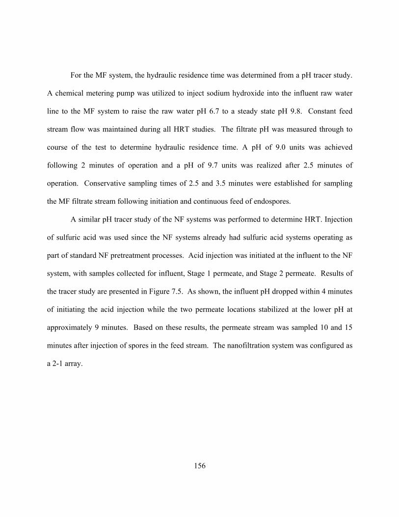
156
For the MF system, the hydraulic residence time was determined from a pH tracer study.
A chemical metering pump was utilized to inject sodium hydroxide into the influent raw water
line to the MF system to raise the raw water pH 6.7 to a steady state pH 9.8. Constant feed
stream flow was maintained during all HRT studies. The filtrate pH was measured through to
course of the test to determine hydraulic residence time. A pH of 9.0 units was achieved
following 2 minutes of operation and a pH of 9.7 units was realized after 2.5 minutes of
operation. Conservative sampling times of 2.5 and 3.5 minutes were established for sampling
the MF filtrate stream following initiation and continuous feed of endospores.
A similar pH tracer study of the NF systems was performed to determine HRT. Injection
part of standard NF pretreatment processes. Acid injection was initiated at the influent to the NF
system
of sulfuric acid was used since the NF systems already had sulfuric acid systems operating as
, with samples collected for influent, Stage 1 permeate, and Stage 2 permeate. Results of
the tracer study are presented in Figure 7.5. As shown, the influent pH dropped within 4 minutes
of initiating the acid injection while the two permeate locations stabilized at the lower pH at
approximately 9 minutes. Based on these results, the permeate stream was sampled 10 and 15
minutes after injection of spores in the feed stream. The nanofiltration system was configured as
a 2-1 array.
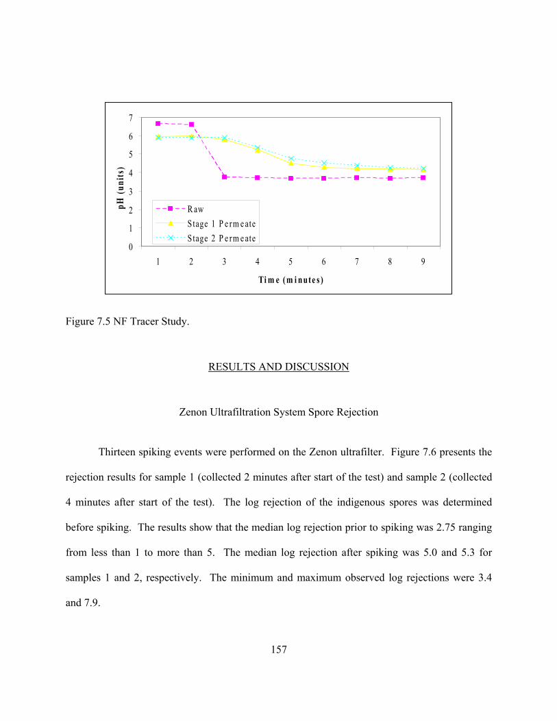
0
1
3
4
6
pH (u
nits
)
2
5
7
1 2 3 4 5 6 7 8 9
Ti m e (m i nute s )
R awStage 1 P e rm e ateStage 2 P e rm e ate
Figure 7.5 NF Tracer Study.
RESULTS AND DISCUSSION
Zenon Ultrafiltration System Spore Rejection
Thirteen spiking events were performed on the Zenon ultrafilter. Figure 7.6 presents the
rejection results for sample 1 (collected 2 minutes after start of the test) and samp d
d
before spiking. The results show that the median log rejection prior to spiking was 2.75 ranging
from le
le 2 (collecte
4 minutes after start of the test). The log rejection of the indigenous spores was determine
ss than 1 to more than 5. The median log rejection after spiking was 5.0 and 5.3 for
samples 1 and 2, respectively. The minimum and maximum observed log rejections were 3.4
and 7.9.
157

0
2
6
8
10
Log
Reva
l
4
Before Spiking Sample 1 Sample 2
mo
Figure 7.6 Media UF System
The indigenous log rejection of spores does not indicate a lower limit of spore rejection
by UF. Aerobic spores may accumulate in permeate lines during operation independently of
challenge events. Consequently, the spores measured during a spiking event represent a
conservative measurement of spore rejection by membrane processes. Nine of thirteen samples
were taken when the ZUF operated without chemical addition, and four samples were taken
when a coagulant was added prior to ZUF. The coagulation occurred in a flocculation tank prior
to the ZUF. The median log rejections for sample 1 and 2 were 5.0 and 5.4 when no coagulant
was used, and 4.2 and 4.9 for sample 1 and 2 when a coagulant was used. There was no change
in system log removal associated with coagulation in this work. Coagulation could potentially
reduce organic concentration in the finished water and organic fouling of all membrane units.
n, Minimum and Maximum Log Rejection of Spores by Zenon
158
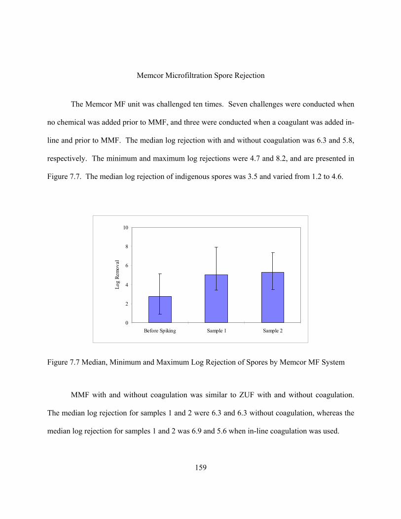
159
Memcor Microfiltration Spore Rejection
The Memcor MF unit was challenged ten times. Seven challenges were conducted when
no chemical was added prior to MMF, and three were conducted when a coagulant was added in-
line and prior to MMF. The median log rejection with and without coagulation was 6.3 and 5.8,
respectively. The minimum and maximum log rejections were 4.7 and 8.2, and are presented in
Figure 7.7. The median log rejection of indigenous spores was 3.5 and varied from 1.2 to 4.6.
0
2
4
6
8
10
ova
l
Before Spiking Sample 1 Sample 2
Lg
Rem
o
Figure
The median log rejection for samples 1 and 2 were 6.3 and 6.3 without coagulation, whereas the
7.7 Median, Minimum and Maximum Log Rejection of Spores by Memcor MF System
MMF with and without coagulation was similar to ZUF with and without coagulation.
median log rejection for samples 1 and 2 was 6.9 and 5.6 when in-line coagulation was used.

160
ed for these tests due to the documented presence of indigenous
spores in the permeate lines prior to spiking events. Additionally, spores or any contaminate
with an average size greater than the nominal pore size of any membrane can pass the membrane
due to variation in membrane pore sizes. Additionally, absolute rejection can not be claimed by
any water treatment process including membranes even if indigenous microorganisms are not
present following treatment. However, the median rejection of either MF exceeded the
regulatory credits for Giardia rejection (2.5 log removal) (USEPA, 1991).
Fluid Systems CALP Nanofiltration System Spore Rejection
Nine spiking events were performed on the CALP Fluid Systems mem ranes. Samples
each permeate location, at 10 and 15 minutes after spiking was initiated. The results are
present
Total rejection of spores was not achieved for either microfiltration systems. Total spore
rejection could not be achiev
b
were collected on Stage 1 permeate and Stage 2 permeate. Two samples were obtained from
ed in Figure 7.8. The median log rejection of Stage 1 was 2.4 and 2.2 whereas the median
log rejection of Stage 2 was 3.2 and 3.2 at 10 and 15 minutes, respectively.
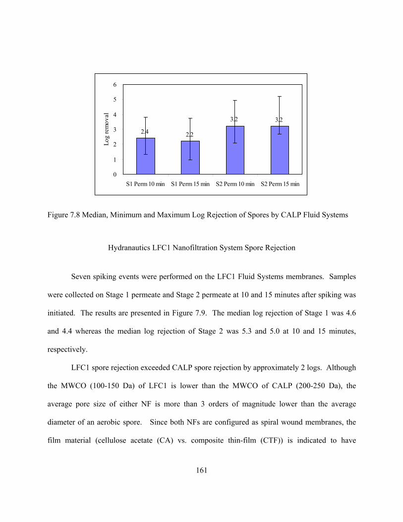
2.4 2.2
1
2
3
4
5
S1 Perm 10 min S1 Perm 15 min S2 Perm 10 min S2 Perm 15 min
Lg
rem
val
3.2 3.2
0
6
oo
s
Hydranautics LFC1 Nanofiltration System Spore Rejection
Seven spiking events were performed on the LFC1 Fluid Systems membranes. Samples
were collected on Stage 1 perm
membranes, the
film material (cellulose acetate (CA) vs. composite thin-film (CTF)) is indicated to have
Figure 7.8 Median, Minimum and Maximum Log Rejection of Spores by CALP Fluid System
eate and Stage 2 permeate at 10 and 15 minutes after spiking was
initiated. The results are presented in Figure 7.9. The median log rejection of Stage 1 was 4.6
and 4.4 whereas the median log rejection of Stage 2 was 5.3 and 5.0 at 10 and 15 minutes,
respectively.
LFC1 spore rejection exceeded CALP spore rejection by approximately 2 logs. Although
the MWCO (100-150 Da) of LFC1 is lower than the MWCO of CALP (200-250 Da), the
average pore size of either NF is more than 3 orders of magnitude lower than the average
diameter of an aerobic spore. Since both NFs are configured as spiral wound
161
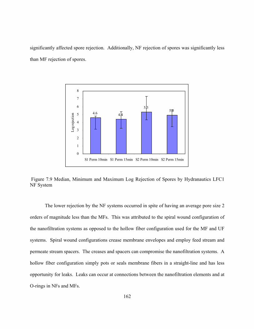
162
significantly affected spore rejection. Additionally, NF rejection of spores was significantly less
than MF rejection of spores.
4.6 4.4
5.35.0
0
1
2
3
4
5
6
7
8
S1 Perm 10min 10min S2 Perm 15min
Log
reje
ctio
n
S1 Perm 15min S2 Perm
Figure 7.9 Median, MinimNF Sys
r at connections between the nanofiltration elements and at
O-rings in NFs and MFs.
um and Maximum Log Rejection of Spores by Hydranautics LFC1 tem
The lower rejection by the NF systems occurred in spite of having an average pore size 2
orders of magnitude less than the MFs. This was attributed to the spiral wound configuration of
the nanofiltration systems as opposed to the hollow fiber configuration used for the MF and UF
systems. Spiral wound configurations crease membrane envelopes and employ feed stream and
permeate stream spacers. The creases and spacers can compromise the nanofiltration systems. A
hollow fiber configuration simply pots or seals membrane fibers in a straight-line and has less
opportunity for leaks. Leaks can occu

163
e likewise too large to pass the second stage membranes. Hence, log
rejection of spores will increase as stages increase because the feed stream concentration is
higher because of the addition of easily rejected s
individual IMS unit operations. Eight different IMSs were previously identified and as
vary for all IMSs (four of eight) involving different
log removal varied from 8.0 to 11.0 logs and exceeded the credited 2.5 log rejection for Giardia
NF spore rejection in the second stage was higher for both the LFC1 and CALP systems
than in first stage. This will typically be the case for all staged NF systems when contaminants
are rejected by size exclusion, which is typically the case for microorganism rejection by NF.
The feed stream concentration to the second stage is the reject or concentrate stream from the
first stage, which will include all of the rejected contaminates from the first stage and will be
more concentrated. As the spores rejected by the first stage were too large to pass the first stage
membranes, they ar
pores.
Integrated Membrane Systems
Log rejection of an integrated membrane system (IMS) is the sum of the log rejections of
previously shown in-line coagulation had no effect on spore rejection in these results. However,
as shown Figure 7.10, spore rejection did
membrane systems. The average log rejection of ZUF and MMF were 5.2 and 6.0, respectively.
The average log rejection of CALP and LFC1 were 2.8 and 5.0, respectively. IMS cumulative
of conventional treatment systems. The results are presented in Figure 7.10.
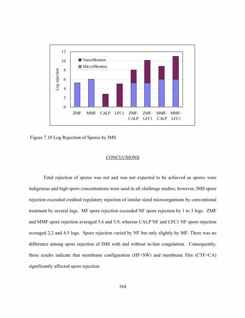
0ZMF MMF CALP LFC1 ZMF- ZMF- MMF- MMF-
2
4Log
6
8
10jec
tion
12
CALP LFC1 CALP LFC1
reNanofiltrationMicrofiltration
Figure 7.10 Log Rejection of Spores by IMS
CONCLUSIONS
Total rejection of spores was not and was not expected to be achieved as spores were
hallenge studies; however, IMS spore
. ZMF
here was no
these results indicate that membrane configuration (HF>SW) and membrane film (CTF>CA)
indigenous and high spore concentrations were used in all c
rejection exceeded credited regulatory rejection of similar sized microorganisms by conventional
treatment by several logs. MF spore rejection exceeded NF spore rejection by 1 to 3 logs
and MMF spore rejection averaged 5.6 and 5.9, whereas CALP NF and LFC1 NF spore rejection
averaged 2.2 and 4.5 logs. Spore rejection varied by NF but only slightly by MF. T
difference among spore rejection of IMS with and without in-line coagulation. Consequently,
significantly affected spore rejection.
164
165
water community and regulatory acceptance. These results demonstrated rejection of a smaller
ent selection and the NF
membrane systems.
REFERENCES
The ability to quantify the removal efficacy of a water treatment technology is critical for
and viable microbial surrogate for Cryptosporidium by separate and integrated membrane
systems, which exceeded log removal credits given for conventional treatment. IMS log
reduction of cyst sized microorganisms is dependent on pretreatm
membrane film, which should be considered by any utility evaluating separate or integrated
Facing Microfiltration and Ultrafiltration,
5 American Water Works Association Membrane
ce as an Alternative Filtration Technology”,
s Responsible for
Fox K. R. and Lytle, 1996. The Milwaukee Cryptosporidiosis Outbreak: Investigation and Recommendations, J. AWWA, 88, 87.
Adham, S., Trussell R. S., Gagliardo P. F., and Trussell R. R., Sept. 1998. “Rejection of MS-2 Virus by RO Membranes, Jour. AWWA, 90:9:130.
Allgeier, S., 2001, Overview of Regulatory IssuesProceedings of the AWWA Membrane Conference, San Antonio, TX.
Alspach, B. and Allgeier, S., Mar. 2005. “The Membrane Filtration Guidance Manual - Overview and Update”, Proceedings of the 200Technologies Conference, Phoenix, AZ.
Askenaizer, D., Sakaji, R., Jacangelo, J., Mar. 2005. “California’s Approach to Assignment of Pathogen Removal Credits and Membrane AcceptanProceedings of the 2005 American Water Works Association Membrane Technologies Conference, Phoenix, AZ.
Colvin, C. K., Acker, C. L., Marinas, B. J. and Lozier, J. C. 1999. Mechanismthe Passage of Microorganisms through RO and NF Membranes, Proceedings of the AWWA Membrane Conference, Long Beach, CA.
166
Glover, N., 1994. “The isolation and identification of Mycobacterium avium complex (MAC) recovered from Los Angeles potable water, a possible source of infection in AIDS patients.” Journal of Environmental Health Research, 4, 63-72.
Hancock, C.M.; J.B. Rose and M. Callahan. 1998. Crypto and Giardia in US Groundwater. J. AWWA, 90:3 58-61.
Hong S., F. Miller, and J. Taylor, 2001. “Assessing Pathogen Removal Efficiency of Microfiltration by Monitoring Membrane Integrity”, Water Science and Technology: Water Supply, 1(4), 43-48.
Hong, S. K., Taylor J. S., Rose, J., Gibbson, C. Owen, C. and Johnson, W., 1999. Removal of Microorganisms by MF Process: Correlation between Membrane Integrity Test Results and Microbial Removal Efficiency, Proceedings of the AWWA Membrane Conference, Long Beach, CA.
Hoxie, N.J.; J.P. Davis; J.M. Vergeront; R.D. Nashold and K.A. Blair., 1997. “Cryptosporidiosis – Associated Mortality Following a Massive Waterborne Outbreak in Milwaukee, Wisconsin.” Amer. J. Public Health 12.
Jacangelo, J.G.; Adham, S.S.; and Laine, J.-M., 1995. “Mechanism of Cryptosporidium, Giardia and MS2 virus removal by MF and UF.” J. AWWA, 87, 9.
Kruithof, J. C., Kamp, P. C., Folmer, H. C., 2001. Membrane Integrity Monitoring at the UF/RO Heemskerk Plant, Proceedings of the AWWA Membrane Conference, San Antonio, TX.
LeChevallier, M.L. 1996. What do Studies of Potable Water System Groundwater Studies Tell Us?”. Proceedings of Groundwater Foundation’s 12th Annual Fall Symposium Under the Microscope: Examining Microbes in Groundwater, Lincoln, NE.
Lisle J.T. and J.B. Rose. 1995. “Cryptosporidium contamination of water in the USA and UK: a mini review.” J. Water Supply & Res. Tech. 44 103.
Lovins W. A, J S. Taylor, S. Hong, 2002. Microorganism Rejection by Membrane Systems, Journal of Environmental Engineering Science, 19:453-465.
Gerba, C.P. and Rose, J.B., 1989. Viruses in Source and Drinking Water. In McFeters, G.A., Ed., Advances in Drinking Water Microbiology Research. Science Tech, Madison, WI.

167
McN an. Proceedings
Novick, R.J., 1990. Nontuberculous Mycobacterial Infections in Hearth Transplant Recipients: a Seventeen Year Experience. J. Heart Transplant, 9, 357-63.
Reiss, C.R. and Taylor, J.S., Mar. 1991. “Membrane Pretreatment of a Surface Water” Proceedings of the AWWA Membrane Conference, Orlando, Florida.
Reiss, C.R. and Taylor, J.S., Aug. 1995. “Prediction of Nanofilter Productivity Decline using
Rice, E.W., Fox, K.R., Miltner, R.J., Lytle, D.A., and Johnson, C.H., 1994. A microbiological surrogaQuality Technology Conference, San Francisco, CA, November 6-9.
Adham, S., Trussell R. S., Gagliardo P. F., and Trussell R. R., Sept. 1998. “Rejection of MS-2
Taylor, J.S., Reiss, C.R., Morris, K.E., Jones, P.S., Smith, D.K., Lyn, T.L. and Duranceau, S.J.,
No. EPA/ 600/ R-92/023.
Taylor, J.S., Reiss, C.R., Robert, C. and Lovins. W.A. November, 1998, “Selection and PerformInstitute Microfiltration Conference. San Diego, CA.
amara, T. D., and Gavin T. C., 1997. Microfiltration. Case Study; Marquette, Michg of the AWWA Membrane Conference, New Orleans, LA.
Fouling Indices”, Proceedings of the AWWA Membrane Specialty Conference, Reno, NV.
Reiss, C.R., Taylor, J.S., Robert, C., and Lovins, W., Mar. 1999. “Pathogen, Taste & Odor, Turbidity and DBP-precursor Removal by Surface Water Membrane Systems”, Proceedings of the South Carolina Environmental Conference. Myrtle Beach, SC.
te for evaluating treatment efficiency.“ American Water Works Association Water
Virus by RO Membranes, Jour. AWWA, 90:9:130.
Seyde, V., Clark, D., Akiyoshi, E., Kalinsky, A. and Spangenberg, C., Feb. 1999. “Nanofiltration Process Microbial Challenge Studies” Proceedings of the AWWA Membrane Technologies Conference, Long Beach, CA.
Feb. 1992. Reduction of Disinfection By-Product Precursors by Nanofiltration, USEPA Report
ance of Integrated Membrane Systems”, Proceedings of National Water Research
United States Environmental Protection Agency, National Primary Drinking Water Standards, 40CFR, Section 143, Federal Regiser, January, 1991.

168
Denitrification and Organic Matter Removal in Drinking Water. Proceedings of the AWWA Urbain, V. and Manhem J., 1997. Membrane Bioreactor Technologies for Disinfection,
Membrane Conference, New Orleans, LA.

169
CHAPTER 8 CONTROL OF TASTE AND ODOR COMPOUNDS BY MEMBRANE SYSTEMS
INTRODUCTION
Control of taste and odor compounds in drinking water supplies represents a key
s. Suffet et al. (1993) reported that 22% of the water
providers surveyed in a United States study reported taste and odor problems in their source
waters. The presence of objectionable taste and odor in drinking water represents an aesthetic
issue resulting in customer complaints.
The most significant source of odor in water supplies is the growth and decay of
microorganisms in surface water. Blue-green algae, green algae, diatoms, and flagellates are four
in (trans-1,10-dimethyl-trans-decalol) is an
odor-causing metabolite produced by blue-green algae, which possess an earthy, musty smell.
Moldli
United
States
treatment objective for many municipalitie
algae groups responsible for odor complaints. Geosm
ke bacteria called actinomycetes are also present in surface water and produce 2-
methylisoborneol (MIB), another odor compound (Rashash, D., 1994). Geosmin and MIB
represent the primary compounds responsible for taste and odor present in surface waters
throughout the world (Durrer et al. 1999; Graham et al., 2000).
There is no known health-related regulation associated with taste and odor. The
Environmental Protection Agency (USEPA) has set a secondary standard of 3 units for
Threshold Odor Number (TON), an aggregate measure of the odor of water, for aesthetic
purposes (USEPA, 1991). The World Health Organization Drinking Water Quality Guidelines
170
indicate
geosmi
ounds and
associa
uire, 1986; Izaguirre and Taylor, 1995).
er control methods
include
that the taste and odor of drinking water should not be offensive to the consumer,
however, no health-based guideline value is proposed (WHO, 2004). The Ames test has been
widely used since the 1970s as a preliminary screening tool for potential carcinogens. Neither
n nor MIB are mutagenic as determined by the Ames test (Dionigi et al. 1993; Nakajima
et al. 1996), which has limited research.
However, the need for research into the presence of taste and odor comp
ted control methods is important. Taste and odor compounds are detected at very low
concentrations. The average person detects geosmin at 4 nanograms per litre (ng/L) and MIB at
9 ng/L. (Ndiongue et al., 2004). Taste and odor problems have been traced to planktonic and
benthic algae in water supplies, canals, surface impoundments, and distribution networks
(Izaguirre et al., 1982; Means and McG
Control of taste and odor can be challenging. MIB and geosmin have stable ring
formations that make bond-cleaving difficult (Figure 8.1 and Figure 8.2). Therefore, MIB and
geosmin are difficult to oxidize or to degrade microbiologically (Jung et al., 2004; Durrer, 1999;
Saito et al., 1999).
Coagulation can not remove MIB and geosmin effectively. Oth
oxidation by chlorine, chlorine dioxide and ozone, granular activated carbon (GAC) and
powdered activated carbon (PAC) adsorption, and gamma radiation (Jung et al., 2004, Duarte, et
al., 2002).

OHCH3
171
3CH
Molecular weight: 182.31 daltons
H 12.16% O 8.78% Boiling Point: 260°C
C 79.06%
Figure 8.1 Geosmin Molecular Structure.
Molecular weight: 168.28 daltons C 78.51% H 11.98% O 9.51% Boiling Point: 207°C
C H 3
C H 3
3
O H C H H 3 C
Figure
dor. Ozone, GAC and
PAC are used ahead of MF or UF to remove taste and odor compounds, and are required since
MF or UF removes no dissolved compounds (G an, 2005; Kelly et al., 2003).
The process train for the Region of Peel, Canada 95.4 MGD water treatment plant on
Lake O
8.2 2-Methylisoborneol Molecular Structure.
Membrane technologies represent an additional potential method of taste and odor
control. Size-exclusion controlled processes such as microfiltration (MF) and ultrafiltration (UF)
have been utilized as part of multi-unit process trains to control taste and o
arcia-Alem
ntario is ozone-biologically active carbon-UF. Ozone and biologically active carbon
were selected, in part, for their ability to control taste and odor that would otherwise pass through
the UF membrane (Garcia-Aleman, 2005).

172
) or nanofiltration
(NF) can remove low molecular weight dissolved molecules such as taste and odor compounds.
However, little is know and odor.
N RO syste te osm l
from the s source for the Yuciapa Valley Region ter Filtrati . S NF
and RO m es were tested, and n and MIB removals from 50 to 99% were reported.
No inform n influent or finis ater geosmin IB conc tions or challenge
testin lt et al.,
In addition to a general lack of information on RO and NF taste and odor removal, the
research to-date h in, which omits
critically high events ith seasonal changes in sou uality. Cha sting
with higher concentrations of MIB and geosmin provides an opportunity for conservative
assessments of t e expected from membrane systems.
The research presented herein evaluated the ability technolo rol
taste and od able water quality surface supply in Tam lorida.
This pilot testing documented the removal of taste and odor compounds at ambient conditions as
well as
In summarizing UF pilot testing performed in France, Virginia, and Texas, Kelly et al.
(2003) acknowledge the need to add appropriate unit process(es) when taste and odor removal is
required and described the benefit of using powdered activated carbon.
Diffusion-controlled membrane processes such as reverse osmosis (RO
n about the capability of RO or NF to remove taste
Alt et al. used bench-scale F and ms to evalua MIB and ge in remova
urface al Wa on Facility even
embran geosmi
ation o hed w and M entra
g was reported (A 2005).
as focused on ambient concentrations of MIB and geosm
associated w rce water q llenge te
he limits of performanc
o f membrane gies to cont
or when treating a highly vari pa, F
removal capabilities when challenged with high concentrations of MIB and geosmin
artificially introduced into the feed water.

173
METHODS AND MATERIALS
Source Water
The source water for this research was the Hillsborough River in Tampa, Florida. The
Tampa Water Department owns and operates the David L. Tippen Water Treatment Plant (DLT
WTP), a 120 mgd (454 ML/d) conventional ferric coagulation, sedimentation, filtration (CSF)
water treatment plant (WTP) that was the site for this pilot study project. The Hillsborough
River is a spring-fed river with supplemental supply coming from precipitation and watershed
runoff. Water quality varies greatly between seasons with higher organic levels and lower TDS
during the wet (summer) season and higher TDS and lower organic levels during the dry (winter)
season.
Water quality during the 15 months of pilot operation is presented in Table 8.1. These
water quality analyses were performed by City of Tampa Laboratory personnel. As shown, taste
and odor values varied over the course of the study. TON averaged 10.1 units, suggesting water
with a high potential for taste and odor complaints unless adequate treatment is provided. Both
geosmin and MIB were present, averaging 4.6 and 5.6 ng/L, respectively.
Pilot Systems
Four different membrane pilot units were operated at the DLT WTP site in Tampa,
Florida, treating raw water from the Hillsborough River. One MF system was used and consisted
of a 10 gpm pressurized, hollow fiber system manufactured by US Filter/Memcor. One UF

174
system was used and consisted of a 10 gpm, immersed, hollow fiber system manufactured by
Zenon. Both the MF and UF system are automatic backwash systems that are designed for
removal of turbidity and pathogens from surface waters and were used to directly treat the raw
water from the Hillsborough River. Specifications are provided in Table 8.2.
Table 8.1 Hillsborough River Raw Water Quality
Parameter Units Maximum Minimum Average TON (units) 50.0 1.0 10.1 MIB (ng/L) 25.4 <1 5.6
Geosmin (ng/L) 11.5 <1 4.6 TOC (mg/L) 27.5 4.0 16.4
UV-254 (cm-1) 1.9070 0.1508 0.7412 Color (cpu) 297 34 153
aCO3) 178 30 80 aCO3) 184 50 108
TDS (mg/L) 270 63 169
Alkalinity (mg/L as CTotal Hardness (mg/L as C
Table 8.2 Microfiltration and Ultrafiltration Specifications
Parameter Memcor Zenon Model CMF ZW500
Nominal Pore size (microns) 0.2 0.05
Module configuration Pressurized Immersed 3
Flow configuration Outside-In Outside-In
Active membrane area, A (ft ) 355 150
Fiber configuration Hollow Hollow
Number of Modules 3
Material Polypropylene Proprietary 2
Number of fibers per module NA 1550
The MF and UF systems were used with and without inline coagulation (ILC) of raw
water, which reduced MF or UF system fouling and/or agglomerated dissolved constituents such
as taste and odor compounds to allow filtration and removal. A dose of aluminum sulfate of no
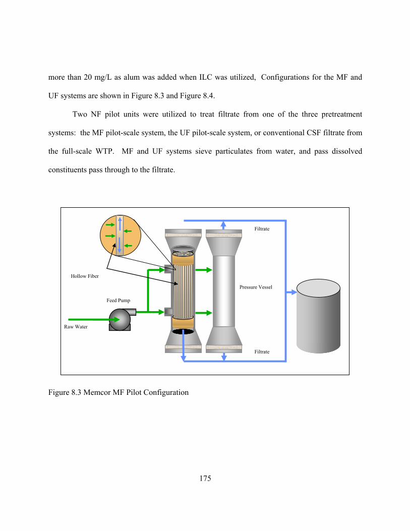
175
ree pretreatment
systems: the MF pilot-scale system, the UF pilot-scale system, or conventional CSF filtrate from
the full-scale WTP. MF a water, and pass dissolved
constituents pass through to the filtrate.
more than 20 mg/L as alum was added when ILC was utilized, Configurations for the MF and
UF systems are shown in Figure 8.3 and Figure 8.4.
Two NF pilot units were utilized to treat filtrate from one of the th
nd UF systems sieve particulates from
Feed Pump
Raw Water
Filtrate
Filtrate
Pressure Vessel
Hollow Fiber
Figure 8.3 Memcor MF Pilot Configuration
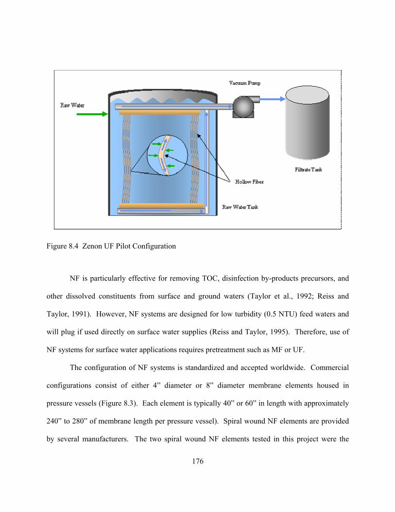
176
Figure 8.4 Zenon UF Pilot Configuration
res pretreatment such as MF or UF.
The configuration of NF systems is standardized and accepted worldwide. Commercial
configurations consist of eith r membrane elements housed in
pressure vessels (Figure 8.3). Each element is typically 40” or 60” in length with approximately
240” to 280” of membrane length per pressure vessel). Spiral wound NF elements are provided
by several manufacturers. The two spiral wound NF elements tested in this project were the
NF is particularly effective for removing TOC, disinfection by-products precursors, and
other dissolved constituents from surface and ground waters (Taylor et al., 1992; Reiss and
Taylor, 1991). However, NF systems are designed for low turbidity (0.5 NTU) feed waters and
will plug if used directly on surface water supplies (Reiss and Taylor, 1995). Therefore, use of
NF systems for surface water applications requi
er 4” diameter or 8” diamete
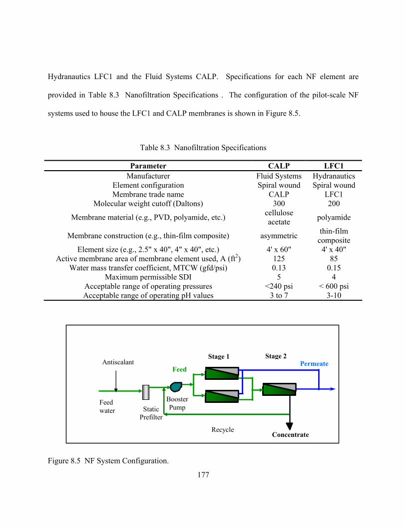
Hydranautics LFC1 and the Fluid Systems CALP. Specifications for each NF element are
provided in Table 8.3 Nanofiltration Specifications . The configuration of the pilot-scale NF
systems used to house the LFC1 and CALP membranes is shown in Figure 8.5.
Table 8.3 Nanofiltration Specifications
Parameter CALP LFC1 Manufacturer Fluid Systems Hydranautics
Element configuration Spiral wound Spiral wound Membrane trade name CALP LFC1
cellulose
thin-film
Element size (e.g., 2.5" x 40", 4" x 40", etc.) 4' x 60" 4' x 40" lement used, A (ft2) 125 85
Water mass transfer coefficient, MTCW (gfd/psi) 0.13 0.15
Acceptable range of operating pressures <240 psi < 600 psi
Molecular weight cutoff (Daltons) 300 200
Membrane material (e.g., PVD, polyamide, etc.) acetate polyamide
Membrane construction (e.g., thin-film composite) asymmetric composite
Active membrane area of membrane e
Maximum permissible SDI 5 4
Acceptable range of operating pH values 3 to 7 3-10
Booster Pump
Concentrate
Permeate
Feed water
177
Feed
Static Prefilter
Antiscalant Stage 1 Stage 2
Recycle
igure 8.5 NF System Configuration. F

178
Ambient Performance Evaluation
The four membrane pilot units and the filtrate from the conventional WTP were paired to
form six different process trains. These six process train configurations were operated at the
DLT WTP in Tampa, Florida and assessed for control of taste and odor compounds. The UF,
MF, LFC1, and CALP systems were continuously operated for approximately 1 year at 10, 15,
10, and 10 gpm, respectively. A side stream of filtrate from the CSF WTP was utilized as feed
for the CSF-NF experiments. The UF system was tested with and without in-line alum
coagulation. The six process trains were:
UF→CALP NF UF→LFC1 NF MF→CALP NF MF→LFC1 NF CSF→CALP NF CSF→LFC1 NF
Ambient concentrations of MIB, geosmin, and TON were measured biweekly. The
purpose of this testing was to document the taste and odor control capabilities of each unit
process as well as the combined process train, over a multi-season period. Documentation of
removal capabilities of NF systems in particular is very limited, and this data provided a long-
term assessment of performance.
Challenge Testing Evaluation
allenge testing of the NF systems
was performed. While it was known that removal of taste and odor compounds by CSF, MF, or
UF systems would likely be limited, the capabilities of NF for removal of low molecular weight
In addition to the ambient performance evaluation, ch

179
taste and odor compounds was potentially very high, but are poorly documented. Therefore, a
series of tests were performed on each NF system at various flux and recovery settings.
Reagent-grade MIB and geosmin solutions were prepared and injected into the feed stream of
each NF system to provide a minimum of 100 ng/L of each compound in the feed water. This
represents a conservative, challenging evaluation of the performance of the LFC1 and CALP
nanofilters to reject these low molecular weight compounds. Samples were collected and
analyzed for the spiked feed water, NF permeate from Stage 1, and NF permeate from Stage 2.
Two flux and two recovery settings were selected, to evaluate the variation in rejection
capability of each compound and assess the degree that diffusion was controlling rejection. Each
NF system was tested at fluxes of 7 and 14 gfd (12 and 24 L/m /hr) and recoveries of 65% and
85% for four experiments on each NF.
Based on the solution diffusion theory, models have been developed to predict permeate
concentration. The linear model (Equation (8.1)) incorporates solution diffusion theory and
predicts that permeate concentration would increase with decreasing flux and increasing
recovery (Taylor, 1996). The linear model has been used to predict pesticide rejection (Chen et
al., 2004; Duranceau et al., 1992) and operational effects (Reiss et al., 2001) on mass transfer in
diffusion controlled membrane systems. This model was used to determine if diffusion
controlled the permeation of MIB and geosmin through the NF membranes.
2
ss
sfp
Kr22r2J
KCC
+⎟⎠⎞
⎜⎝⎛
−−
= (8.1)

180
Where:
Cf = feed concentration, mg/L
r = water recovery (%/100)
The pilot units were in continuous operation at normal operational settings throughout the
course of the challenge testing. Spiking of MIB and geosmin to each NF system was based on
the volume of pretreated water fed to the train and the concentration of MIB and geosmin in the
stock solution. The stock solution was injected into the feed stream at a rate as was theoretically
required to obtain at least 100 ng/L in the spiked feed water (Figure 8.6).
Permeate Feed water Feed
Stage 1 Stage 2
Recycle
Injection
Sampling Point
Sampling Point
NF System
Figure 8.6 MIB and Geosmin Addition and Sampling Points
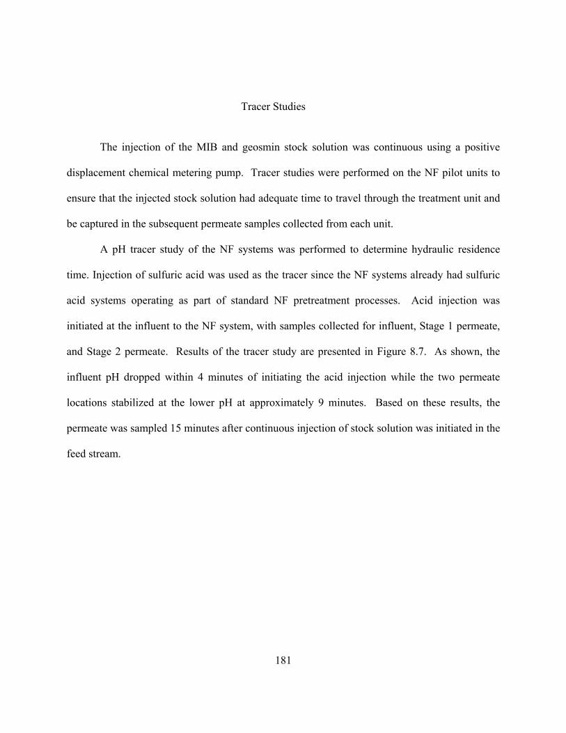
181
The injection of the MIB and geosmin stock solution was continuous using a positive
displacement chemical metering pump. Tracer studies were performed on the NF pilot units to
ensure that the injected stock solution had adequate time to travel through the treatment unit and
be capt
Tracer Studies
ured in the subsequent permeate samples collected from each unit.
A pH tracer study of the NF systems was performed to determine hydraulic residence
time. Injection of sulfuric acid was used as the tracer since the NF systems already had sulfuric
acid systems operating as part of standard NF pretreatment processes. Acid injection was
initiated at the influent to the NF system, with samples collected for influent, Stage 1 permeate,
and Stage 2 permeate. Results of the tracer study are presented in Figure 8.7. As shown, the
influent pH dropped within 4 minutes of initiating the acid injection while the two permeate
locations stabilized at the lower pH at approximately 9 minutes. Based on these results, the
permeate was sampled 15 minutes after continuous injection of stock solution was initiated in the
feed stream.
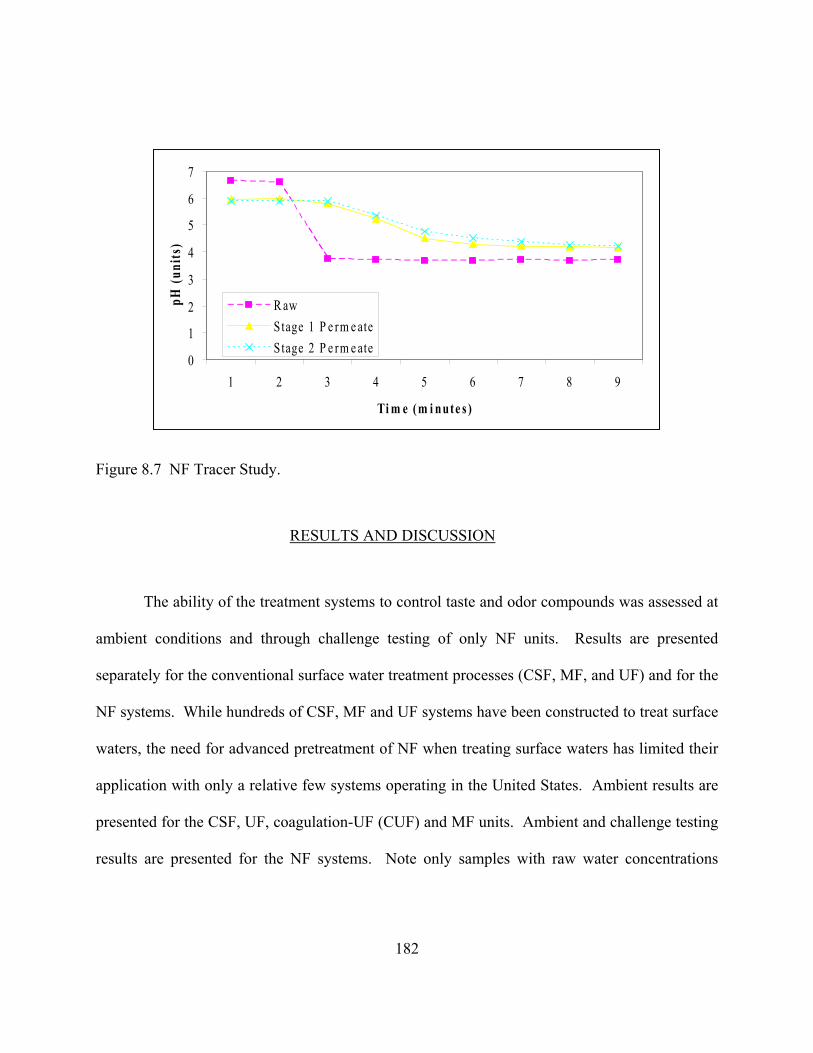
0
1
2
3
4
5
6
7
1 2 3 4 5 6 7 8 9
Ti m e (m i nute s )
pH (u
nits
)
R awStage 1 P e rm e ateStage 2 P e rm e ate
Figure 8.7 NF Tracer Study.
RESULTS AND DISCUSSION
The ability of the treatment systems to control taste and odor compounds was assessed at
ambient conditions and through challenge testing of only NF units. Results are presented
separately for the conventional surface water treatment processes (CSF, MF, and UF) and for the
NF systems. While hundreds of CSF, MF and UF systems have been constructed to treat surface
waters, the need for advanced pretreatment of NF when treating surface waters has limited their
application with only a relative few systems operating in the United States. Ambient results are
presented for the CSF, UF, coagulation-UF (CUF) and MF units. Ambient and challenge testing
results are presented for the NF systems. Note only samples with raw water concentrations
182

183
Conventional Surface Water Treatment System Results
The TON in the raw water and CSF, MF and UF filtrate is shown in Figure 8.8 for the
ambient tests. Raw water ambient TON was highest (26 ng/L) when CSF was evaluated, and
approximately 7 when UF, CUF and MF were evaluated. Removal of TON by one of the
conventional surface water treatment and the size exclusion membrane processes (CSF, MF, or
UF) varied from 18 to 72 percent. CSF provided the highest removal of 72 percent. This was as
expected, since the CSF WTP utilized potassium permanganate, high doses of ferric sulfate, and
free chlorine as part of the treatment process. MF and UF provided very limited removal (18 to
30 percent), as was expected for these processes, which do not significantly remove disso ed
l TON removal as shown in Figure 8.8.
Most important to note regarding these treatment processes is that none could
consistently meet the USEPA TON secondary standard of 3 units for this source water, in which
raw water TON was measured as high as 50 units and the average during testing of the CSF was
22 units.
above the detection limit are considered in these results as they allow assessment of removal
capabilities of the treatment processes.
lv
compounds. Coagulation preceeded the UF system (CUF) for a portion of the time, but did not
provide additiona
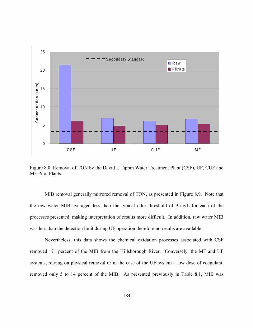
0
5
1 0
1 5
2 0
2 5
C S F U F C U F M F
Con
cent
ratio
n (u
nits
)
R a wF iltra te
S e c o nda ry S ta nda rd
Figure 8.8 Removal of TON by the David L Tippin Water Treatment Plant (CSF), UF, CUF and MF Pilot Plants.
to 14 percent of the MIB. As presented previously in Table 8.1, MIB was
MIB removal generally mirrored removal of TON, as presented in Figure 8.9. Note that
the raw water MIB averaged less than the typical odor threshold of 9 ng/L for each of the
processes presented, making interpretation of results more difficult. In addition, raw water MIB
was less than the detection limit during UF operation therefore no results are available.
Nevertheless, this data shows the chemical oxidation processes associated with CSF
removed 71 percent of the MIB from the Hillsborough River. Conversely, the MF and UF
systems, relying on physical removal or in the case of the UF system a low dose of coagulant,
removed only 5
184

185
measured in concentrations up to 25.4 ng/L in the raw water. During these periods, only the CSF
process would be able to meet the 9 ng/L threshold standard.
BD L0
1
2
3
4
5
6
7
8
9
10
C SF U F C U F MF
Con
cent
ratio
n (n
g/L)
R awFiltra te
Typica l M IB Threshold
Figure 8.9 Removal of MIB by the David L Tippin Water Treatment Plant (CSF), UF, CUF and MF Pilot Plants.
Geosmin removal is presented in Figure 8.10 and exemplifies the limits of MF and UF to
raw water geosmin concentrations
between 2.3 and 6.6 ng/L, CSF removed 78% of geosmin. MF and UF removed between 28 and
42 percent of geosmin. With on of 11.5 ng/L, the typical
geosmin threshold of 5 ng/L would only reliably be met by the oxidation enchanced CSF plant
process.
remove dissolved taste and odor compounds. With average
a maximum raw water concentrati
0
1
2
4
5
C SF U F C U F
Con
cent
3
7
M F
ratio
n ( 6
8
9
10
ng/L
)
R awFiltra te
Typica l G eosmin Threshold
Figure 8.10 Removal of Geosmin by the David L Tippin Water Treatment Plant (CSF), UF, CUF and MF Pilot Plants.
A summary of the removal percentages by pretreatment process is presented in Figure
8.11. As described, CSF provides a higher removal of TON, MIB and geosmin, over MF and UF
processes. This can be attributed to the use of potassium permanganate and free chlorine as well
as coagulants in the CSF process. Addition of low doses of coagulant (less than 20 mg/L as
alum) into the UF system did not provide significant additional removal. The removal of taste
and odor compounds by MF and UF are higher than might be expected given that taste and odor
is more commonly associated with dissolved compounds. It is likely that particulate and
colloidal removal by MF and UF corresponded with the partial reduction in taste and odor
concentrations.
186

While CSF showed substantial removal of taste and odor, taste and odor objectives have
not always been met during extreme events. This is consistent with experiences at the site
facility and other conventional surface water treatment facilities throughout the United States
that report taste and odor as an treatment issue. Integration of RO or NF with other treatment
processes can improve finished water quality.
BDL0%
10%
20%
30%
40%
50%
60%
70%
80%
90%
C SF U F C U F M F
Rem
oval
TO NM IBG eosmin
Figure 8.11 Percent Removal of Ambient Taste and Odor Compounds by the David L Tippin Water Treatment Plant (CSF), UF, CUF and MF Pilot Plants.
ter Quality Results NF Ambient Wa
Removal of ambient taste and odor compounds by NF was evaluated over an extended
period of time with samples collected at the influent to the NF systems as well as the combined
187

188
ieved various filtrates from the CSF, MF, and UF
pretreatment systems. The average feed and permeate concentrations of TON, MIB and geosmin
throughout the testing period are discussed in the following text..
As shown in Figure 8.12, reduction in TON levels by NF were significant and resulted in
values less than the secondary standard of 3 units for both the CALP and the LFC1 nanofilter.
Note that average feed water concentrations were less than 6 units due to the reductions achieved
by upstream pretreatment processes. However, these results support the ability of NF to polish
filtrate from conventional surface water treatment systems to meet TON goals.
permeate. Results are presented in Figure 8.12, Figure 8.13 amd Figure 8.14 for TON, MIB and
geosmin, respectively. The NF systems rec
0
1
2
3
C A L P L F C 1
Cnc
ent 4
5
6
8
9
1 0
ora
tion
(uni
t
7
s)
F e e dF iltra te
S e c o nda ry S ta nda rd
Figure 8.12 Removal of Ambient TON by NF
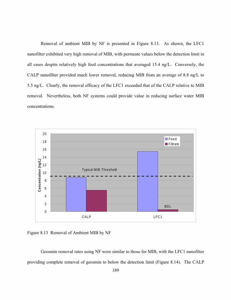
189
aged 15.4 ng/L. Conversely, the
CALP nanofilter provided much lower removal, reducing MIB from an average of 8.8 ng/L to
5.5 ng/L. Clearly, the removal efficacy of the LFC1 exceeded that of the CALP relative to MIB
removal. Nevertheless, both NF systems could provide value in reducing surface water MIB
concentrations.
Removal of ambient MIB by NF is presented in Figure 8.13. As shown, the LFC1
nanofilter exhibited very high removal of MIB, with permeate values below the detection limit in
all cases despite relatively high feed concentrations that aver
BD L0
2
4
6C
8
10
12
14
16
18
20
C ALP LFC 1
once
ntra
tion
(ng/
L)
FeedFiltra te
Typical M IB Threshold
Figure 8.13 Removal of Ambient MIB by NF
providing complete removal of geosmin to below the detection limit (Figure 8.14). The CALP
Geosmin removal rates using NF were similar to those for MIB, with the LFC1 nanofilter

190
nanofilter provided credible but lower removal, with the average feed water geosmin
concentration reduced to less than 2.1 ng/L.
BD L
0
1
2
3
4
6
7
8
9
10
trat
on (
L)
5
C ALP LFC 1
Con
cen
ing
/
FeedFiltra te
Typical G eosmin Threshold
Figure 8.14 Removal of Ambient Geosmin by NF
The removal of ambient taste and odor compounds by NF are summarized in Figure 8.15.
As show, the CALP nanofilter provided 40 to 50 percent removal and the LFC1 removed 58 to
97 percent of the ambient TON, MIB and geosmin. Although high, MIB and geosmin removal
was limited by the feed concentration. These results show the difference between nanofilters for
removal of taste and odor. The CALP, a cellulose acetate based membrane, rejected less ambient
TON, MIB and geosmin than did the polyamide composite based LFC1. Similar results have
microorganisms. (Lovins et al., been observed for rejection of inorganic solutes, TOC and

191
2003). This is important for communities with severe taste and odor concerns and the need for
high levels of treatment or for surface water systems with limited upfront removal of taste and
odor, such as those that use a stand-alone MF or UF system.
> 97%> 89%
50%
60%
70%
80%
100%
oval
0%
10%
20%
30%
40%
90%
C ALP LFC 1
Rem
TO NM IBG eosmin
Figure 8.15 Percent Removal of Ambient Taste and Odor Compounds by NF
NF Challenge Test Results
To better understand the limits of removal using NF, challenge tests were performed with
addition of MIB and geosmin to the feed water. Concentrations of 100 ng/L for each compound
were targeted. Results are presented in Figure 8.16 and Figure 8.17 for average removal of MIB
and geosmin, respectively.

The CALP feed MIB concentration averaged 137 ng/L with the combined permeate
averaging 88 ng/L. This consists of an average removal rate of 37 percent, which is consistent
with the average of 37 percent removal obtained for the ambient water analysis. The removal
capabilities of the CALP nanofilter did not vary with feed concentration. The LFC1 feed MIB
concentration averaged 110 ng/L with the permeate concentration averaging 1 ng/L. Note that
measurable concentrations of MIB were detected in the LFC1 permeate, indicating that the
removal limit of the LFC1 was reached at the 110 ng/L feed concentration. Nevertheless, these
results indicate that the LFC1 could be used for any natural surface water to provide near
complete removal of MIB and would meet MIB goals.
0
20
40
60
80
100
120
140
160
atio
n (n
g/L)
CALP LFC1
Con
cent
r
FeedPermeate
Figure 8.16 Average Removal of Challenge Test MIB by NF
192
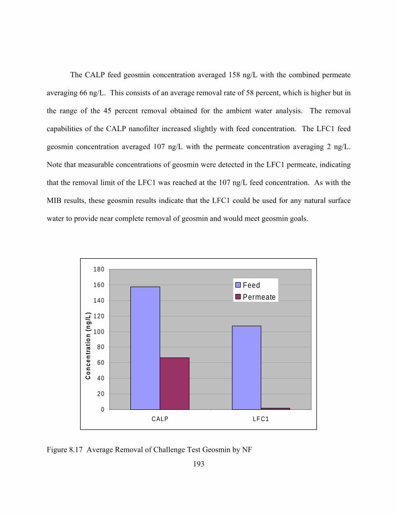
193
hich is higher but in
the range of the 45 percent removal obtained for the ambient water analysis. The removal
capabilities of e LFC1 feed
geosmi eate con
Note that measurable concentrations of geosmin were detected in the LFC1 permeate, indicating
that the removal limit of the LF as reached at 107 ng/L feed centration. As with the
MIB res ese geosmin results indicate that the LFC1 could be used for any natural surface
water to provide near complete removal of geosmin and would meet geosmin goals.
The CALP feed geosmin concentration averaged 158 ng/L with the combined permeate
averaging 66 ng/L. This consists of an average removal rate of 58 percent, w
the CALP nanofilter increased slightly with feed concentration. Th
n concentration averaged 107 ng/L with the perm centration averaging 2 ng/L.
C1 w the con
ults, th
0
20
40
60
80
100
120
140
160
180
CALP LF C1
Con
cent
ratio
n (n
g/L)
FeedPermeate
Figure 8.17 Average Removal of Challenge Test Geosmin by NF

194
While average results were presented above, a total of four experiments were performed
for each nanofilter, representing two flux and two recovery settings. Detailed results by
experiment are presented in Table 8.4. For assessment of the degree of influence due to
diffusion and for mathematical prediction of the expected permeate concentration, the linear
homogenous solution diffusion (LHSD) model was solved for KS, the solute mass transfer
coefficient. Four data points were available for each analyte, by membrane. The resulting
values are presented in Table 8.5. As shown, three of the four conditions did not converge. This
indicates that diffusion plays a limited role, if any, in the reduction of MIB and geosmin using
the two NF systems tested. The LHSD model would not be appropriate for determining the
effect of operating condition on permeate water quality.
Rejection of MIB and geosmin molecules in the CALP and LFC1 nanofilters appears to
be driving by size exclusion. Geosmin and MIB have molecular weights of approximately 182
and 168 daltons, respectively, which suggests greater removal would be achieved by the 200
molecular weight cutoff (MWCO) LFC1 nanofilter versus the 300 MWCO CALP nanofilter, as
was realized. In addition, these molecular weights are an order of magnitude larger than solutes
more commonly found to be diffusion controlled in NF and RO systems, such as sodium and
chloride.
However, previous research has shown that organic parameters including TOC, color and
UV-254 are diffusion controlled for the LFC1 and CALP NF (Reiss et al., 1999). The inability
to document diffusion-controlled rejection could be explained for the LFC1 membrane by the
low permeate concentrations, which approached the detection limit of 1 ng/L. However, the
CALP permeate concentrations were sufficiently high yet diffusion effects were not observed.

195
This further supports a size exclusion mechanism of removal. The absence of a significant
charge associated with the MIB or geosmin molecule is likely a key factor.
Table 8.4 MIB and Geosmin Concentrations by Operating Condition
Flux/ Recovery MIB (ng/L) Geosmin (ng/L) (gfd/%) Feed Permeate Feed Permeate
CALP 7/65 158 113 174 84 7/85 118 75 162 66 14/65 135 87 154 77 14/85 137 68 140 37
LFC1 7/65 142 1 144 2 7/85 102 3 103 1 14/65 154 1 96 3 14/85 140 1 86 2
Table 8.5 Solute Mass Transfer Coefficients
CALP LFC1 Ks(gfd) Converged Ks(gfd) Converged
MIB 3.89E+08 No 0.04 Yes Geosmin 3.6 No 0.034 No
CONCLUSIONS
Reduction of taste and odor compounds by CSF, MF, or UF was only significant when
oxidation and coagulation were employed. Solely using porous filtration in the form of MF or
UF membrane systems resulted variable removal between 5 and 40 percent. These results held
true for removal of TON, MIB, and geosmin. None of the three treatment technologies could
consistently meet the USEPA TON secondary standard of 3 units for this source water, in which

196
raw water TON was measured as high as 50 units and the average during testing of the CSF was
22 units.
Advanced surface water treatment in the form of NF, a semipermiable filtration
technology, resulted in significant and consistent removal of TON, MIB, and geosmin. This
technology requires advanced pretreatment for application on surface waters therefore would be
most applicable as a polishing step following conventional surface water treatment.
A cellulose acetate nanofilter consistently removed 35 to 50 percent of TON, MIB, and
geosmin. However, this would still not provide assurance of compliance the TON standard of 3
units.
A polyamide nanofilter provided over 99 percent removal of MIB and geosmin,
representing the most capable system evaluated. Use of polyamide NF to support compliance
with taste and odor objectives offers significant benefits for continuous and high levels of
removal.
Challenge tests using MIB and geosmin and operating at various nanofilter flux and
recovery settings was performed. Application of the homogeneous solution diffusion equation
was performed to determine if rejection of taste and odor compounds by NF is diffusion control.
Results indicate that size-exclusion drives removal of taste and odor compounds, based on the
data available.
197
REFERENCES
Alt, S., Vickers, J., Zoba, J., Pafundi, D., March 2005. “Bench-Scale Evaluation of Low Rejection Nanofiltration Membranes for DBP Control at the Yucaipa Valley Water District”, Proceedings of the 2005 AWWA Membrane Technology Conference. Phoenix, AZ.
Chen S-S, J. S. Taylor , L. A. Mulford and C. D. Norris, Jan. 2004. "Influences of molecular weight, molecular size, flux, and recovery for aromatic pesticide removal by nanofiltration membranes", Desalination, Volume 160, Issue 2, 15, Pages 103-111
Dionigi, C.P., Lawlor, T.E., McFarland, J.E. and Johnsen, P.B., 1993. Evaluation of geosmin and 2-methylisoborneol on the histidine dependence of TA98 and TA100 Salmonella typhimurium tester strains. Wat. Res., 27(11), 1615-1618.
Duarte, C. L, Sakagami, M.K, Mautone, C.A, de Oliveira Sampa, M.H., Borrely,S.I., Somessari, E.S., Oct. 2002. Removal of Odorifc substances in Drinking Water Caused by Seaweed Using Ionizing Radiation, Proceedings of the Americas Nuclear Energy Symposium, Coral Gables, FL.
Duranceau, S. J., Taylor, J. S., 1992. A SOC Removal in a Membrane Softening Process, Jour. of AWWA, 84:1:68.
Durrer, M.; Zimmermann, U.; Juttner, F., 1999. Dissolved and particle-bound geosmin in a mesotrophic lake (lake Zurich): spatial and seasonal distribution and the effect of grazers. Wat. Res., 33:(17), 628-3636.
Garcia-Aleman, J., Mains, K., Farr, A., Mar. 2005.“Integrating 80 MGD of membranes, ozone and biological pretreatment at Lakeview WTP”, Proceedings of the 2005 AWWA Membrane Technology Conference. Phoenix, AZ. .
Graham, M.R; Summers, R.S.; Simpson, M.R.; Macleod, B.W., 2000. Modeling equilibrium adsorption of 2-methylisoborneol and geosmin in natural waters. Wat. Res., 34:(8):2291-2300.
Izaguirre, G., and W.D. Taylor., 1995. Geosmin and 2-methylisoborneol productionin a major aqueduct system. Water Sci. Technol. 31:41-48.
Izaguirre, G., C.J. Hwang, S.W. Krasner, and M.J. McGuire., 1982. Geosmin and 2-methylisoborneol from cyanobacteria in three water supply systems. Appl. Environ. Microbiol. 43:708-714.
198
Kelly, R.F., Colas, F., Bonnelye, V., Tarallo, S., Mar. 2003, “Impact of Ultrafiltration Membrane Material and Precoagulation Strategy on an Enhanced Clarification Process”, Proceedings of the 2003 AWWA Membrane Technology Conference. Atlanta, GA.
William L. A., Taylor J. S., Hong S. K., 2003. Microorganism Rejection by Membrane Systems, Journal of Environmental Engineering Science, 19:453-465.
Means, E.G. III, and M.J. McGuire., 1986. An early warning system for taste and odor control. Journal AWWA, March, 1986: 77-83.
Nakajima, M., Ogura, T., Kusama, Y., Iwabuchi, N., Imawaka, T., Araki, A., Sasaki, T., Hirose, E. and Sunairi, M., 1996. Inhibitory effects of odor substances, geosmin and 2-methylisoborneol, on early development of sea urchins. Wat. Res., 30(10), 2508-2511.
Rashash, Diana., 1994. Identification and Characterization of Odorous Metabolites Produced by Selected Freshwater Algae. Virginia Polytechnic Institute and State University. Blacksburg, VA.
Reiss C. R., J. S. Taylor, C. Robert, and S. Hong, Mar. 2001. "Cumulative Mass-Based Modeling of Nanofiltration Productivity" Proceedings of American Water Works Association 2001 Membrane Technology Conference, San Antonio, Texas.
Reiss, C.R., Taylor, J.S., Robert, C., Owen, C.A., Nov. 1999. Diffusion- Controlled Organic Solute Mass Transport in Nanofiltration Systems. Proceedings of the AWWA Water Quality Technology Conference. Tampa, FL.
Reiss, C.R. and Taylor, J.S., Mar. 1991. “Membrane Pretreatment of a Surface Water” Proceedings of the AWWA Membrane Conference, Orlando, Florida.
Reiss, C.R. and Taylor, J.S., Aug. 1995. “Prediction of Nanofilter Productivity Decline using Fouling Indices”, Proceedings of the 1995 AWWA Membrane Specialty Conference, Reno, NV.
S. Ndiongue, W. B. Anderson, A. Tadwalkar, J. Rudnickas, S. Pillai And P. M. Huck, 2004. Pilot Scale Investigation of the Removal of Geosmin and MIB by Granular Activated Carbon Filtration. Proceedings of the 2004 Thirty-Ninth Central Canadian Symposium On Water Quality Research, February 9 and 10, Burlington, Ontario
S.-W. Jung, K.-H. Baek and M.-J. Yu, 2004. Treatment of taste and odor material by oxidation and adsorption, Water Science & Technology, Vol 49, No 9, 289–295.

199
Saito, A.; Tokuyama, T.; Tanaka, T.; Oritani, T.; Fuchigami, K., 1999. Microbiological degradation of (-)-Geosmin. Wat. Res., 33: (13), 3033-3036.
Suffet, I.H., C. Anselme, and J. Mallevialle. 1993. AWWA Taste and Odor Survey, Proc. AWWA Water Quality and Technology Conference, Miami, FL, 1785-1831.
Taylor, J.S., 1996. Reverse Osmosis and Nanofiltration, in Water Treatment Membrane Processes, ed. P. Jacobs, et al., McGraw-Hill, NY
Taylor, J.S., Reiss, C.R., Morris, K.E., Jones, P.S., Smith, D.K., Lyn, T.L. and Duranceau, S.J., February 1992. Reduction of Disinfection By-Product Precursors by Nanofiltration, USEPA Report No. EPA/ 600/ R-92/023.
United States Environmental Protection Agency, National Secondary Drinking Water Standards, 40CFR, Section 143.3, Federal Regiser, January, 1991.
World Health Organization, Guidelines for Drinking Water Quality, 3rd Edition, Volume 1, Geneva, Switzerland, 2004

200
APPENDIX A RESISTANCE MODELING

201
RESISTANCE MODEL
This appendix is an investigation of fouling. Various equations are used to describe
fouling mechanisms, which are used for modeling mass transfer and fouling. Equation (A.1)
describes the solvent or water flux as a function of the applied pressure and the osmotic pressure,
which results in a concentration gradient between the feed and permeate.
( )A
Q PKJ p
Ww =∆Π−∆= (A.1)
Where:
Jw = water flux (L3/L2t)
∆P = pressure gradient (L), [(Pf+Pc)/2-Pp]
∆Π = osmotic pressure (L) [(Πf+Πc)/2-Πp]
The solvent mass transfer coefficient, Kw, or solvent permeability in Equation (A.2) was
developed from solution-diffusion theory to be a function of a number of factors as follows
(Weber, 1972):
RTlVCDK www
w = (A.2)
Where:
Dw = diffusivity of water in the membrane
Cw = concentration of water in the membrane

202
Vw = molar volume of water
R = gas constant
T = temperature
l = membrane thickness
The solvent mass transfer coefficient can be calculated from operational data and
manipulation of Equation (A.3):
( )∆Π−∆=
PJK w
W (A.3)
The solvent mass transfer coefficient provides a productivity parameter normalized for
both flux and pressure. As shown in Equation (A.3), Kw is proportional to flux and inversely
proportional to pressure. Additionally, Kw is a function of temperature (Equation (A.2)) due to
the change in water viscosity with temperature. Therefore Kw must be normalized for
temperature.
This definition of Kw (Equation (A.2)) represents the membrane in its clean, non-fouled
state. In fact, as a membrane becomes fouled, either the flux drops or the required pressure
increases or both. This is due to a decrease in Kw and can be explained by simple process
dynamics. Traditional process dynamics describe flow rate as follows:
tRFQ = (A.4)

203
Where:
Q = flow rate
F = driving force
Rt = total resistance
Equation (A.1), which describes membrane water flux, can be considered equivalent to
Equation (A.4) for simple process dynamics, where Jw represents a flow rate, (∆P-∆∏) a driving
force and Kw the inverse of resistance. Substituting Kw with a resistance term gives:
( ) ( )T
Ww RPPKJ π∆−∆
=π∆−∆×= (A.5)
Where
= total resistance to solvent transport, 1/Kw
Additionally, Equation (A.5) can be divided by net driving pressure to show the
relationship between Kw and resistance.
RT
( ) TW
w
R1K
PJ
==π∆−∆
(A.6)
In this form, it can be seen that as the resistance increases (due to fouling), the flux, Jw,
will decline or the driving force (pressure) will need increase to maintain flux. In either case, Kw
will decline. This total resistance is due to the factors described in Equation (A.6), which
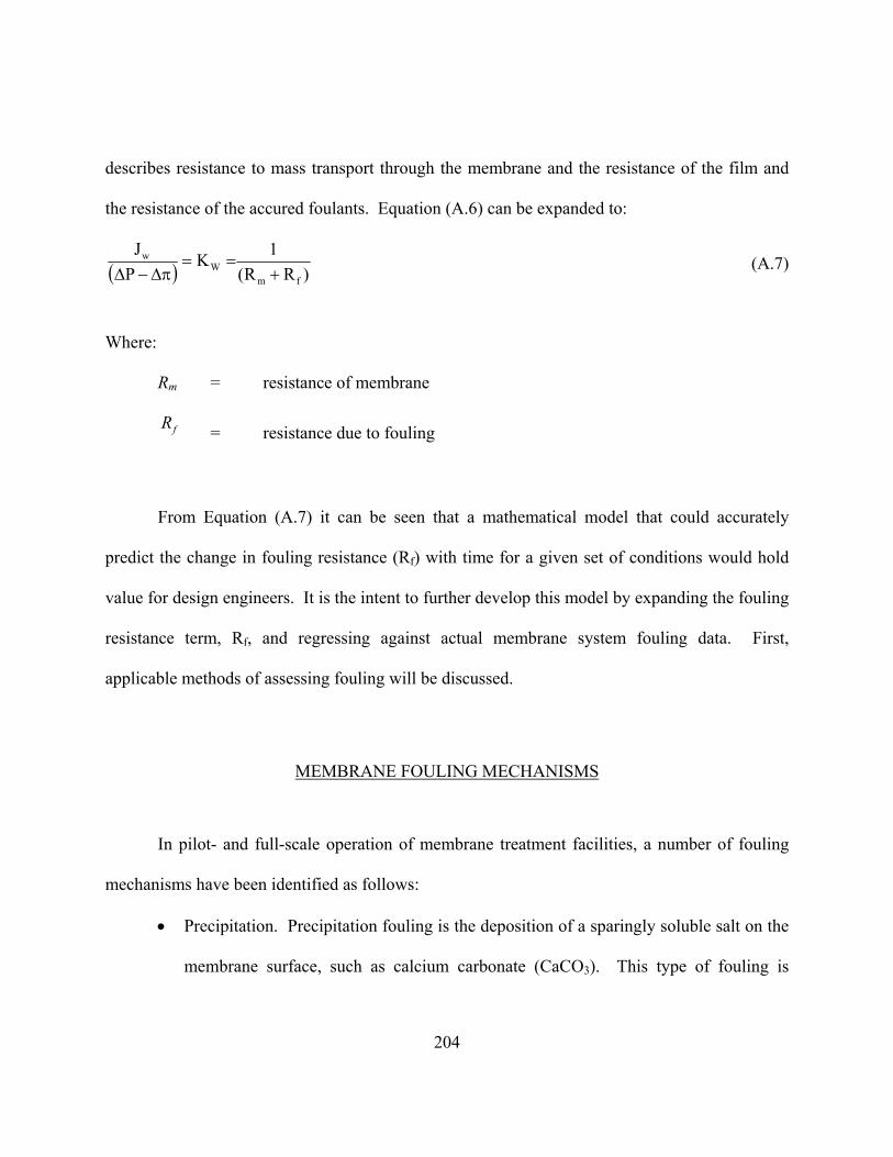
204
describes resistance to mass transport through the membrane and the resistance of the film and
the resistance of the accured foulants. Equation (A.6) can be expanded to:
( ) )RR(1K
PJ
fmW
w
+==
π∆−∆ (A.7)
Where:
Rm = resistance of membrane
= resistance due to fouling
From Equation (A.7) it can be seen that a mathematical model that could accurately
predict the change in fouling resistance (Rf) with time for a given set of conditions would hold
value for design engineers. It is the intent to further develop this model by expanding the fouling
resistance term, Rf, and regressing against actual membrane system fouling data. First,
applicable methods of assessing fouling will be discussed.
MEMBRANE FOULING MECHANISMS
Rf
In pilot- and full-scale operation of membrane treatment facilities, a number of fouling
mechanisms have been identified as follows:
• Precipitation. Precipitation fouling is the deposition of a sparingly soluble salt on the
membrane surface, such as calcium carbonate (CaCO3). This type of fouling is
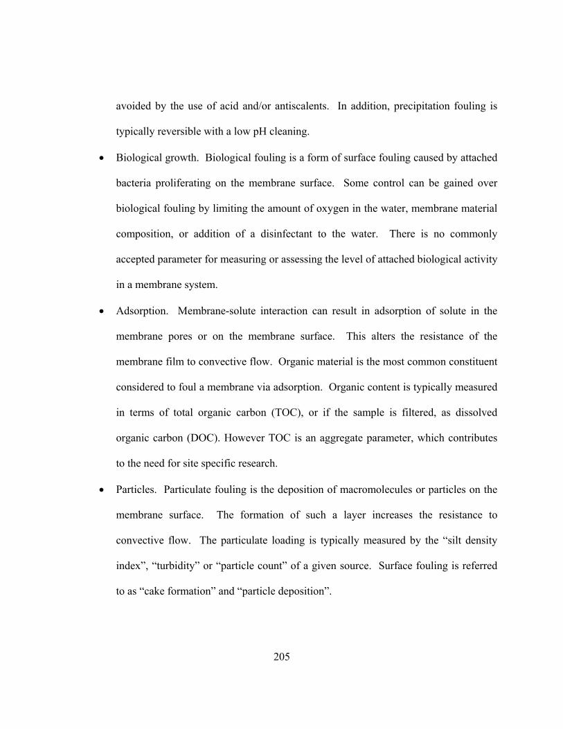
205
avoided by the use of acid and/or antiscalents. In addition, precipitation fouling is
typically reversible with a low pH cleaning.
• Biological growth. Biological fouling is a form of surface fouling caused by attached
bacteria proliferating on the membrane surface. Some control can be gained over
biological fouling by limiting the amount of oxygen in the water, membrane material
composition, or addition of a disinfectant to the water. There is no commonly
accepted parameter for measuring or assessing the level of attached biological activity
in a membrane system.
• Adsorption. Membrane-solute interaction can result in adsorption of solute in the
membrane pores or on the membrane surface. This alters the resistance of the
membrane film to convective flow. Organic material is the most common constituent
considered to foul a membrane via adsorption. Organic content is typically measured
in terms of total organic carbon (TOC), or if the sample is filtered, as dissolved
organic carbon (DOC). However TOC is an aggregate parameter, which contributes
to the need for site specific research.
• Particles. Particulate fouling is the deposition of macromolecules or particles on the
membrane surface. The formation of such a layer increases the resistance to
convective flow. The particulate loading is typically measured by the “silt density
index”, “turbidity” or “particle count” of a given source. Surface fouling is referred
to as “cake formation” and “particle deposition”.

206
Each of these fouling mechanisms can occur in a membrane system treating either a
surface or a ground water. However, precipitation is common in groundwaters due to calcium
carbonate saturation and can be controlled by acid or anti-scalent addition. All pilot- and full-
scale systems use acid and/or antiscalent to control precipitation, including the pilot systems
associated with this research. In addition, precipitation affects operation and necessary treatment
modifications. Therefore, precipitation is relatively easily controlled and will not be addressed
further. The remaining three fouling mechanisms are primary concerns in surface water
membrane treatment.
FOULING ASSESSMENT METHODS
Historically, two common approaches for quantifying fouling have been to evaluate the
feed-side pressure differential as a function of time and to evaluate system throughput (Jw, Kw, or
NDP) as a function of time. The feed-side pressure differential (FSP) is the head loss between
the feed and concentrate streams, as follows:
(A.8)
Fouling can result in an increase in FSP over time, which is caused by blockage of the
feed channel. This may be due to particles, precipitate, microorganism growth, or other
phenomena. However, this type of fouling typically represents a gross blockage of the
membrane element and, for the research conducted herein, was not observed. Instead, fouling of
nanofiltration elements typically affects the surface of the membrane film first, before the entire
∆P P Pfs f c= −

207
channel becomes blocked. The use of FSP is limited because of its lack of relation to surface
fouling.
Surface fouling can be represented by flux and net driving pressure (Jw and NDP) or by
the water mass transfer coefficient, Kw. As fouling occurs, the total resistance to flow increases
or, conversely, the water mass transfer coefficient, Kw, decreases. Generally, Kw is a better
representation of fouling since Jw can vary due to fouling or due to changes in the pressure. As
shown in Figure A.1, a plot of Kw versus time provides an assessment of fouling. Flux could be
plotted versus time, but must be constant during this period. Kw is simply a normalized mass
transfer coefficient with respect to pressure. Given its universal applicability, Kw is the primary
method of representing surface fouling. An example of actual field data is presented in Figure
A.1.
0 .0 0
0 .0 5
0 .1 0
0 .1 5
0 .2 0
0 .2 5
0 .3 0
0 2 0 4 0 6 0 8 0 1 0 0 1 2 0
O pe r at i o nal Ti m e (ho ur s )
Kw
(gfd
/psi
)
Figure A.1 Typical Kw Decline Over Operational Time.

208
In the productivity plot above, Kw decreased from an initial value of 0.11 gfd/psi to 0.05
gfd/psi, representing a 55% loss of productivity. The most common method of quantifying this
decline is to linearly regress Kw with time.
tdt
dKKK WWW O
+= (A.9)
Where:
KW 0 = initial Kw
dKw/dt = rate of change of Kw with time
t = time
Linear regression of Kw will provide a slope, dKw/dt that approximates the rate of
decline. A linear regression may not completely explain the observed trend but is a quick and
common method of quantifying fouling rates. Once the slope is determined, it can be used, in
conjunction with the initial Kw and a target productivity loss, to determine the operational period
between cleanings. For example, the data of Figure A.1 can be fitted linearly as shown in Figure
A.2. Clearly the regression line is not a direct match with the data, but is the most common and
simplest method of quantifying productivity decline.
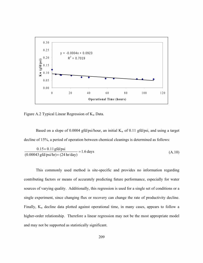
y = -0.0004x + 0.0923R2 = 0.7019
0 .0 0
0 .0 5
0 .1 0
0 .1 5
0 .2 0
0 .2 5
0 .3 0
0 2 0 4 0 6 0 8 0 1 0 0 1 2 0
O pe r at i o nal Ti m e (ho ur s )
Kw
(gfd
/psi
)
Figure A.2 Typical Linear Regression of Kw Data.
Based on a slope of 0.0004 gfd/psi/hour, an initial Kw of 0.11 gfd/psi, and using a target
decline of 15%, a period of operation between chemical cleanings is determined as follows:
days 1.6 hr/day) (24)gfd/psi/hr 00043.0(
gfd/psi 11.015.0=
×× (A.10)
This commonly used method is site-specific and provides no information regarding
contributing factors or means of accurately predicting future performance, especially for water
sources of varying quality. Additionally, this regression is used for a single set of conditions or a
single experiment, since changing flux or recovery can change the rate of productivity decline.
Finally, Kw decline data plotted against operational time, in many cases, appears to follow a
higher-order relationship. Therefore a linear regression may not be the most appropriate model
and may not be supported as statistically significant.
209

210
Mulford et al. (1999) evaluated alternative regressions based on the relationship between
Kw and time. Given that Kw changes with time, zero, first and second order models were
developed from Equation (A.9).
nw
w Kdt
dK= (A.11)
The integrated forms of Equation (A.9) for zero, first and second order are shown in
equations (A.10), (A.11) and (A.12).
Zero Order: Kw = (Kw)o + At (A.12) First Order: Kw = (Kw)oe-A1t (A.13)
Second Order : t2 A)K(
1K1
0ww
+= (A.14)
Where:
Kw = water ma
(Kw)o = initial water mass transfer coefficient (1/day)
A = zero order rate of Kw decline coefficient (1/day2)
A1 = first order rate of Kw decline coefficient (1/day)
A2 = second order rate of Kw decline coefficient
t = cumulative operating time (days)
These models were regressed against actual data to determine which model best describes
productivity with respect to time. The second order model was most representative of fouling for
ss transfer coefficient (1/day)

211
the membrane system evaluated. These results support the resistance model and the intent of this
work is to expand the resistance model and the intent of this dissertation to further develop the
resistance model. Specifically, the three models of Equation (A.10)-(A.12) can be restated as
follows:
Zero Order: AtR1K
MW ±= (A.15)
First Order: tA
MW
1eR1K −= (A.16)
Second Order: tAR
1K2M
W += (A.17)
Comparing these models to the resistance model, reprinted below, it can be seen that a
the second order model most closely resembles the resistance model, with a resistance due to
fouling relationship as shown in Equation (A. 18).
)RR(1K
fmW +
= (A.7)
R A tf = 2 (A. 18)
Given these results, more complex, mechanistic resistance models are developed in this
research. The following sections present fouling research history and the proposed modeling
approach.

212
APPLIED RESEARCH HISTORY
Membrane systems treating surface waters foul extensively but produce very high quality
finished water; hence, fouling mitigation is area of research Studies have shown a difference in
performance between various nanofilters. As a result, research was conducted to characterize
differences in the surfaces of commercially available nanofilters and are described here.
Use of spiral wound nanofiltration and reverse osmosis systems on surface waters with
conventional pretreatment (acid/antiscalent addition and static microfiltration) is rarely viable
and typically results in rapid fouling and shutdown. The primary cause is typically high
concentrations of solids that plug the static cartridge filter. Research efforts have evaluated use
of advanced pretreatment processes ahead of nanofiltration and reverse osmosis systems, in an
effort to extent the operational time between chemical cleanings. The purpose of the advanced
pretreatment processes is to remove foulants before they reach the nanofilter and reduce
productivity. Advanced pretreatment processes have included microfiltration (MF),
ultrafiltration (UF), and coagulation, sedimentation, filtration (CSF). Figure 2.1, presented
previously, illustrates the size ranges of material rejected as a function of separation process.
Figure A.3 illustrates how these pretreatment systems could be used in series with a diffusion-
controlled membrane such as a nanofilter to form an Integrated Membrane System.
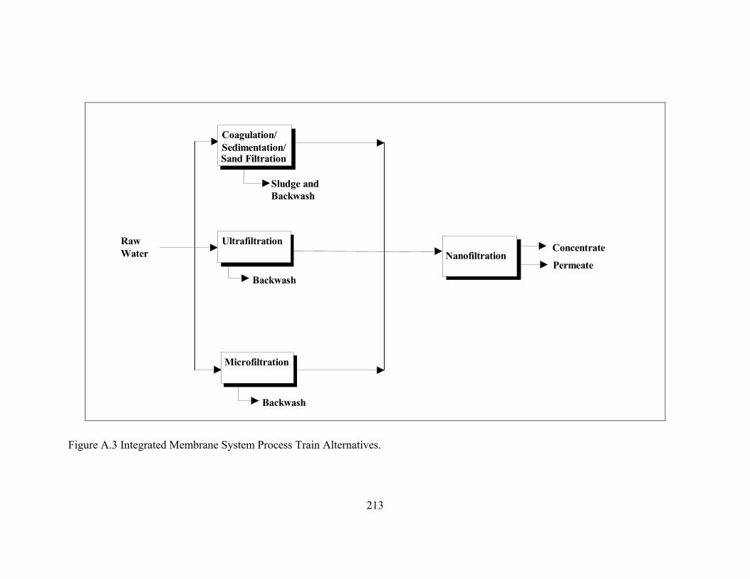
213
Coagulation/Sedimentation/
NanofiltrationPermeate
ConcentrateRawWater
Ultrafiltration
Backwash
Microfiltration
Sand Filtration
Sludge andBackwash
Backwash
Figure A.3 Integrated Membrane System Process Train Alternatives.

214
Micro- and ultra-filtration remove particles in the sub-micron range and should provide
pretreated water with low particle concentrations and fouling. However, these processes do not
remove dissolved organic carbon (DOC), which can foul membranes. Coagulation,
sedimentation, filtration (CSF) will remove a portion of the DOC and the majority of particles.
However, MF and UF processes are generally more effective for removal of particles than CSF..
Pilot-scale research using advanced pretreatment processes shows that nanofilter fouling
rates can be reduced. Taylor et al. (1992) found that pretreatment of a highly organic (TOC ~ 24
mg/L) Florida surface water by either MF or CSF increased nanofilter operational times from
less than 2 hours (with no pretreatment) to as much as three weeks, prior to chemical cleaning.
Chellam et al. (1997) found that pretreatment of a moderately organic (TOC 4-6 mg/L) Virginia
surface water by either MF, UF, or CSF also resulted in nanofiltration operational times between
one and four weeks, before chemical cleaning.
However, full-scale membrane treatment plants using organic groundwater supplies are
capable of operating for 6 months to 3 or more years between chemical cleanings (Reiss et al.
1997a). These waters have naturally low levels of particles. This suggests that high organic
concentrations alone are not responsible for the 1 to 4 week surface water cleaning cycles
experienced. Fouling effects of surface waters have not been fully eliminated by the
pretreatment process trains tested to date, and need to be investigated on a site specific basis.
One explanation for the moderate success of the above studies has been that physical
separation processes such as UF and MF remove particles but do not reduce organic levels while
physical/chemical processes such as CSF do not entirely remove particles or organics. In
addition, none of these pretreatment processes prohibits biological growth within nanofiltration

215
systems. Finally, and most importantly, these studies have not focused on identifying the
particular mechanism, which caused fouling. Understanding the mechanism(s) that are causing
fouling is important for the modeling effort associated with this dissertation and is necessary for
the development of more reliable treatment systems.
In addition to these pilot-scale pretreatment alternatives, laboratory-based work has
evaluated the differences in surface morphology between spiral wound films. The purpose is to
explain the variations in fouling rates that have been observed for different membrane films
treating the same source. Important characteristics with respect to membrane fouling include the
following:
• Membrane material;
• Surface charge; and
• Surface roughness.
Studies have shown differences in fouling rate by membrane material (Speth et al., 1995;
Elimelech et al. 1997). Two primary classes of membrane material are cellulose acetate and
cross-linked aromatic polyamides. These differ significantly in chemical structure and observed
performance. Typical differences are shown in Table A.1.
In addition, research has shown that surface roughness affects particle fouling and surface
charge affects organic adsorption (Elimelech, 1997). However, this work has been laboratory
based; data comparing pilot-scale fouling results with surface characterization results are limited.
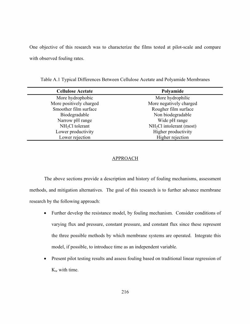
216
One objective of this research was to characterize the films tested at pilot-scale and compare
with observed fouling rates.
Table A.1 Typical Differences Between Cellulose Acetate and Polyamide Membranes
Cellulose Acetate Polyamide More hydrophobic More hydrophilic
More positively charged More negatively charged Smoother film surface Rougher film surface
Biodegradable Non biodegradable Narrow pH range Wide pH range NH2Cl tolerant NH2Cl intolerant (most)
Lower productivity Higher productivity Lower rejection Higher rejection
APPROACH
The above sections provide a description and history of fouling mechanisms, assessment
methods, and mitigation alternatives. The goal of this research is to further advance membrane
research by the following approach:
• Further develop the resistance model, by fouling mechanism. Consider conditions of
varying flux and pressure, constant pressure, and constant flux since these represent
the three possible methods by which membrane systems are operated. Integrate this
model, if possible, to introduce time as an independent variable.
• Present pilot testing results and assess fouling based on traditional linear regression of
Kw with time.
217
• Regress pilot results using various models, including the linear regression of Kw with
time and the resistance model. Modify the models as necessary to fit available data.
Account for variations due to differing conditions, such as different membranes or
use of a biocide.
• Assess the impact of surface characteristics on the rate of fouling and identify
favorable characteristics for future application of membrane technologies
METHODS
Membrane Selection Study
Prior to initiation of the pilot study, a membrane selection study was conducted at
laboratory-scale. Multiple membrane films were evaluated for relative performance and the
most promising membranes selected for pilot testing. This section describes the experimental
plan for the laboratory membrane testing. This includes discussion of the specific experiments
conducted, operational and analytical parameters evaluated and guidelines for data collection and
analytical sampling.
Objectives
The laboratory film testing evaluated multiple membrane films using a flat sheet cell unit
and raw water samples from the Hillsborough River. The objective of these experiments was to
select the most applicable membranes for pilot-scale testing based on data generated in a

218
laboratory setting. Specifically, water mass transfer coefficient, Kw,, and permeate water quality
for various membrane films was determined by cell testing.
General Approach
Water was transported from Tampa to the UCF laboratory in 55-gallon high density
polyethlyene barrels and stored at 4°C in a walk-in cooler. Cell testing was conducted using ten
flat sheet membrane films, denoted Set A, specifically selected for the Tampa site. Raw water
was used for Set A evaluations. Operational and water quality data were collected. and
compared to pre-established goals. Those membranes that failed to produce the water quality
goals were eliminated. The remaining films were evaluated using water quality and water mass
transfer coefficients. Four membranes were selected, which were designated Set B, and were
retested for a expanded list of water quality parameters using raw and coagulated/settled/filtered
water. These results were used to select two membranes for use at pilot scale.
Water Samples
Raw and coagulated/settled/filtered water samples were collected from Tampa on
September 12, 1996. Two 55-gallon samples of raw water and a 55-gallon sample of CSF water
were collected and transported to UCF in non-metallic containers at ambient temperature. The
following analyses were done on-site at the time of sample collection:
• Temperature
• pH
• Turbidity
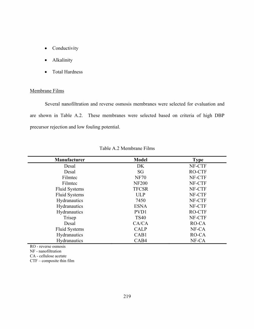
219
• Conductivity
• Alkalinity
• Total Hardness
Membrane Films
Several nanofiltration and reverse osmosis membranes were selected for evaluation and
are shown in Table A.2. These membranes were selected based on criteria of high DBP
precursor rejection and low fouling potential.
Table A.2 Membrane Films
Manufacturer Model Type Desal DK NF-CTF Desal SG RO-CTF
Filmtec NF70 NF-CTF Filmtec NF200 NF-CTF
Fluid Systems TFCSR NF-CTF Fluid Systems ULP NF-CTF Hydranautics 7450 NF-CTF Hydranautics ESNA NF-CTF Hydranautics PVD1 RO-CTF
Trisep TS40 NF-CTF Desal CA/CA RO-CA
Fluid Systems CALP NF-CA Hydranautics CAB1 RO-CA Hydranautics CAB4 NF-CA
RO - reverse osmosis NF - nanofiltration CA - cellulose acetate CTF – composite thin film

220
Equipment
Experiments were conducted using a flat sheet cell unit manufactured by Desalination
Systems, Inc. The cell unit contains two cells, each with 12.6 in2 active membrane area. Feed
flow of approximately 0.3 gpm per cell is supplied by a single 1/3 hp pump. A cartridge
filtration unit pretreats the feed water. A schematic of the cell unit is shown in Figure A.4.
Experimental Conditions
Each membrane film was evaluated once at 15 gallons per square foot-day (gsfd) flux and
one- percent recovery. The surface ares of the films was 12.6 in2. . Each experiment was
continued until 0.5 and 1.4 liters of permeate have been collected for Set A and Set B
experiments, respectively. Flows for 15 gsfd flux and one percent recovery were 3.5 ml/min
permeate and 345 ml/min concentrate for a 12.6 in2 membrane surface area. Operational data
was collected during the course of each experiment and consisted of recording the feed,
permeate, and concentrate flow and pressure every thirty minutes. Raw water was filtered with a
static 1.0 µm filter to remove suspended solids prior to tesing. The pH was not adjusted.

Cartridge
Filter Cell # 1
Cell # 2
Permeate Permeate
Bypass
Membrane
Pressure Valve
Temperature & pH
Pump Flow
Flow
Concentrate ConcentrateConcentrate as Recycle
Tank
Figure A.4 Cell Testing Unit.
These water quality analyses from the flat sheet tests are presented in Table A.3 with maximum desired concentrations as determined by UCF. These maximum concentrations represented UCF's recommendations for water quality goals. All films were tested in Set A using raw water. Selected films were tested in Set B using raw and coagulated/settled/filtered waters.

222
Table A.4 presents a sampling schedule for these parameters at the desired sampling
locations.
Evaluation Criteria
The films were evaluated based on the following criteria:
• Ability to met the established water quality objectives for all parameters (Table A.3)
• Relative permeate concentrations
• Relative "clean membrane" productivity (Kw)
Four membranes were selected from Set A results and tested using the expanded set of
water quality parameters. The same criteria listed above were used for selection of two
membranes for use at pilot scale.
Table A.3 Water Quality Goals
Parameter Units Goal Absolutes pH units 7-9 -
temperature degrees C - - alkalinity mg/L as CaCO3 20-100 -
Total hardness mg/L as CaCO3 20-100 - turbidity ntu < 0.1 < 0.2
particle counts #/ml < 150 - Color cpu 0 < 1 TOC mg/L < 0.5 < 2 Br- µg/L < 0.1 -
UV-254 cm-1 - - Iron mg/L < 0.01 < 0.05
manganese mg/L < 0.01 < 0.05

223
nitrate mg/L < 5 < 10 Silt Density Index units < 1 < 5
SDS-THM µg/L - < 40 SDS-HAA µg/L < 25 < 30 SDS-TOX mg/L < 100 -

224
Table A.4 Sampling Locations
Parameter Units Set A Set B Reservoir Reservoir Settled Water
pH units √ √ √ temperature degrees C √ √ √ alkalinity mg/L as CaCO3 √ √ √
Total hardness mg/L as CaCO3 √ √ √ turbidity ntu √ √ √
Color cpu √ √ √ TOC mg/L √ √ √ Br- µg/L √ √ √
UV-254 cm-1 √ √ √ Iron mg/L √ √ √
manganese mg/L √ √ √ nitrate mg/L √ √ √
Silt Density Index units √ √ SDS-THM µg/L √ √ SDS-HAA µg/L √ √ SDS-TOX mg/L √ √
Concentration Effect on Feed Water
The cell test unit was configurated to return the concentrate stream to the feed tank,
resulting in an increase in feed water concentration over time. Based on a 110-gallon supply of
raw water and 15 scheduled experiments, no more than 7.0 gallons of water was used per
experiment, which controlled concentration of the feed water to acceptable levels. The cell unit
contains a 10-gallon feed water tank. A chiller coil maintained ambient temperature in the feed
tank.
225
Seven gallons of raw water were placed in the feed tank and two samples of the same
film were placed in the test cell for simultaneous evaluation. The water remaining in the feed
tank was disposed of following each experiment and a fresh aliquot of raw water used for the
next experiment. For Set A experiments, a total of 0.5 L of permeate water was removed from
the tank. This represents 2 percent of the original 26 L of raw water in the feed tank. Assuming
100 percent rejection of a contaminant there was a 2 percent increase in the feed water
concentration from the beginning of an experiment to the end. For Set B experiments, a total of
1.4 L of permeate water was removed from the tank. This represents a 5 percent increase in
concentration of the feed water from the beginning to the end of an experiment. These increases
in concentration were acceptable for this evaluation.
Standard Methods and Protocols
The cell testing protocol was as follows:
The flat sheet membranes will be handled according to each manufacturer’s instructions.
The instructions presented with the membranes will be strictly adhered to and the specific
procedure documented in the project logbook at the time of experimentation. The procedures for
the handling of the specific individual membranes will be incorporated into this document as
they are received. In general the shiny side of the membrane sheet is the membrane film and
should be facing the feed side of the flat sheet cell.
The flat sheet cells have a permeate distribution sheet and a porous support filter. The
mounting order of the cell layers starting from the permeate side will be as follows:
226
• Perforated support disc lays on the cell base plate.
• Place the 4-inch porex disc with shiny side down on the perforated support disc.
• Cut to fit borosilicate microfiber filters to cover the 4-inch cell area extending outside
the 0-ring seal.
• Cut the membrane film to cover the 4-inch cell area extending outside the 0-ring seal.
The mounting of the membranes incorporates the use of borosilicate 0. 7 um TCLP grade
filter paper as the specific backing for the membranes. Filter paper is required as a backing and
the TCLP grade is required to minimize contaminant adsorption and interference with analytical
measurements. To ensure a proper seal on the 4-inch diameter effective surface area of the cell,
the filters will be cut to an approximately 5-inch diameter.
Each flat sheet unit has two cells that are operated in parallel. Each cell will hold a
different membrane film but are operated simultaneously to expedite operation. After the
membranes and cell apparatus has been set up, the reservoir is filled with 3.5 gallons of raw
water. The unit is activated and the operating conditions set as described in the experimental
plan section herein. The permeate stream is discarded during the time taken to set the operating
conditions and for at least the first 15 minutes of operation. This clears any organic
preservatives that may be on the film. The concentrate stream is discharged to the reservoir.

227
MODEL DEVELOPMENT
Nanofilter fouling was described previously by the resistance model, reprinted below.
Fouling mechanisms of concern were identified as particle fouling, organic adsorption, and
biofouling. Assuming the resistance model and the foulants are accurate representatives of
nanofilter fouling, a more useful model of productivity decline would be as shown by Equation
(A.20).
( )KJ
P RWw
m f=
−=
+∆ ∆π1
( )
R (A.19)
( ) ( )KJ
P R R R Rw
w
m ads part bio
=−
=+ + +∆ ∆π
1 (A.20)
Where:
Rads = resistance due to adsorption
Rpart = resistance due to particulate fouling
Rbio = resistance due to biogrowth
Each of these resistances are a function of the water volume that passes through the
membrane film.

228
Particulate Fouling
The resistance of a layer of particles to fluid flow as shown in Equation (A.21) is a
function of the specific resistance of the particulate matter, or cake, the weight of dry cake solids
per unit volume of filtrate, and the volume of water filtered. This cake resistance can be
described as follows (Weber 1972; Green and Belfort, 1980).
Rr C V
Apartpart S= (A.21)
Where:
Rpart = resistance due to particulate fouling
CS = concentration of solids in the bulk solution
r = specific resistance of cake
V = cumulative permeate volume
A = surface area of active membrane film
Based on the above equation, the resistance due to particulate fouling increases with
volume as a cake layer builds on the membrane surface. Specific resistance is assumed to be a
constant, therefore is not affected by compression effects. In this model, resistance would
always increase with volume, provided the feed water contained solids. There have been
adaptations to this model by other researchers to describe a non-linear rate of particulate fouling
as has been observed in some experimental data. One limitation of this model is that it does not
account for the shear effect of the concentrate stream passing along the surface of a nanofilter.

229
In fact, some experimental data shows that shear and resuspension of the particulate cake can
result is a steady state water where particulate fouling no longer increases with volume. Theories
that have attempted to explain this include the “lateral migration phenomena”, “revised standard
filtration model”, “particle trajectory analysis”, and “inertial lift theory” (Green and Belfort,
1980; Chellam, 1995). These theories all address a cessation of particle deposition or a
suspension of particles equal to the rate of deposition. Never the less, Equation (A.21) provides
a basic description of increased resistance due to increased particle accumulation on the
membrane surface.
Adsorption
The rate at which dissolved organic substances are removed from aqueous solutions by
solid adsorbents is controlled by one of three steps (Weber, 1972). The three steps in adsorption
are “film diffusion”, “pore diffusion”, and adsorption of the solute on the interior surfaces
bounding the pore and capillary spaces of the adsorbent. Film diffusion refers to mass transfer in
the region separating a bulk solution and a solid surface. A number of theories have described
this phenomena including the film, penetration, and boundary layer theories. These theories all
describe the resistance to mass transfer at the surface of the particle or solid. The second step,
pore diffusion, refers to the diffusion of the adsorbate within the pores of the adsorbent. The
final step is the adsorption of the solute on the interior surfaces bounding the pore and capillary
spaces of the adsorbent. Only one of these three steps is rate-limiting .in every adsorption
system,. Weber (1972) states that the final step, in most processes, is most likely not rate-
230
limiting. For systems with sufficient turbulence, “pore diffusion” can control the rate of uptake.
For continuous flow systems, such as beds of activated carbon treating water, Weber states that
film diffusion is most likely the rate-limiting step.
For a membrane system with water passing across and through the membrane film, it is
not readily evident which step controls adsorption. However, given the relatively low water flux
rates and low Reynolds numbers (typically <200) in membrane systems, film diffusion may be
the controlling step.
For processes controlled by film diffusion, the adsorption rate is proportional to the first
power of concentration (Faust and Aly, 1983). Zogorski showed that the adsorption of 2,4-
dichlorophenol by activated carbon is controlled by film-diffusion at concentrations less than 400
µmol/L, and that a direct linear relationship existed between the initial concentration and the
adsorption rate. Based on a first power relationship, Equation (A.22) describes the effect of
organic adsorption on resistance in a membrane system.
Rr C V
Aadsads O= (A.22)
Where:
Rads(t) = resistance due to adsorption at time t
rads = specific resistance of adsorbed organic carbon
CO = concentration of adsorbable organic carbon
V = cumulative permeate volume
A = surface area of active membrane film
231
This model is developed assuming that the need for a chemical cleaning of the membrane
system is reached before the adsorptive capacity of the membrane material is exhausted (i.e.
equilibrium is never reached). Given that full-scale systems clean at a 10 to 15 percent decline in
productivity, this may be valid. However, the specific resistance of adsorbed material to passage
of water through the membrane is unknown. Never the less, this model describes a relationship
between resistance to water flux and the rate of organic adsorption.
Biogrowth
The growth of microorganisms in a membrane system begins with the attachment of one
or more organisms that reproduce and spread across the membrane surface to form a biological
film. The resistance of this biofilm to water transport through the membrane film can be
modeled as shown in Equation (A.23), which assumes a first order reaction for organism growth
as determined by observed yield from available substrat:
Rr C Y V
Abiobio A obs= (A.23)
Where:
Rbio(t) = resistance due to biogrowth at time t
rbio = specific resistance of biofilm
CA = concentration of assimilable organic carbon
Yobs = observed specific yield coefficient (ratio of the mass of cells formed to the mass of substrate consumed)

232
V = cumulative permeate volume
A = surface area of active membrane film
This model assumes that attached biological growth is initiated immediately upon startup
of the system and is limited by the mass of substrate that passes through the membrane film.
This latter assumption is considered valid given the low concentrations of AOC found in surface
waters.
An alternative approach is to assume to use of a biocide for biological growth control.
For this research monochloramine was used as a bioinhibitor. Monochloramine has the potential
to reverse the effects of fouling, depending upon the chemistry between the microorganisms and
the membrane film and is the primary constituent used in some chemical cleanings solutions.
However, polyamide composite membranes typically have limited tolerance to oxidants;
specifications associated with commercial membranes typically include the maximum acceptable
exposure, in units of mg/L*minutes. For a membrane that is damaged by exposure to an oxidant,
Kw and Ks would be expected to increase. An empirical model based on monochloramine dose
can be developed as follows:
Rr C V
Abiobio Cl= (A.24)
Where:
CCl = concentration of monochloramine (M/L3)

233
The coefficient for this term would be expected to be negative as resistance would
decrease with increasing monochloramine mass. Additionally, for a membrane damaged by
monochloramine, this term would represent the combined effect of reduced resistance due to
oxidation.
Mechanism-Based Modeling Summary
Equations (A.22) - (A.24) can be combined with Equation (A.21) to yield a Kw model
incorporating all three fouling mechanisms as follows:
( )KJ
PR
r C VA
r C VA
r C Y VA
ww
mpart S ads O bio A obs
=−
=+ + +
⎛⎝⎜
⎞⎠⎟
∆ ∆πµ
1(A.25)
This model is acceptable for use with systems operated at constant flux; constant
pressure; or variable flux and pressure. The cumulative volume accounts for the rate of foulant
accumulation of all foulants, irrespective of flux or pressure settings. The concentrations of each
foulant represents the feed-side average concentration therefore recovery is taken into account.
It would be of value to quantify the effect of each fouling mechanism as described and defined
above, and to determine the relative significance of those mechanisms in surface water fouling.
Such a model was utilized in this work.
234
Flux and Net Driving Pressure Considerations
Though Equation (A.25) above is applicable to all flux and pressure conditions, it would
be of interest to simplify this model, if possible, to eliminate the cumulative volume term, V, and
replace with time. This is desirable since, for membrane systems, operating time is more
commonly ;monitored than cumulative volume. Cumulative volume is dependent on surface
area (which is fixed), flux, and net driving pressure (NDP). Three potential operational scenarios
are as follows:
• Constant flux, variable pressure. For systems requiring a consistent water production,
flux is set to a constant value therefore the required NDP will increase as fouling
occurs;
• Variable flux, constant pressure. For systems operating at a constant pressure, flux
will decline as fouling occurs;
• Variable flux and variable pressure. For systems that set the initial conditions and
allow the system to vary freely, fouling will cause a decline in flux and potentially an
increase in NDP.
Based on these situations, three versions of the resistance model were developed. In
addition, two versions of the resistance model with Jw as the dependent variable were developed.
Jw was the dependent variable since Jw supports the mathematical steps for model integration and
represents membrane productivity, in conjunction with pressure. The potential models are
identified by condition in Table A.5.

235
Table A.5 Theoretical Fouling Models by Condition
Model Dependent Variable Jw constant? NDP constant? M1 Jw No No M2 Kw No No M3 Jw No Yes M4 Kw No Yes M5 Kw Yes No
Each of the above models must first be developed then fitted with actual data to
determine their applicability. The models are developed in the following sections, and assume
net driving pressure (NDP), defined as ( )∆ ∆πP − , is a singular variable with no sub variables of
concern.
Model M1 – Flux for Variable Flux and Variable NDP
Equation (A.26) represents Model M1. This equation, as it is written, can be fitted, via
least squares estimation (LSE), to actual data, which provides a means of evaluating how well
flux is described as a function of the net driving pressure, (∆P-∆π), feed-side contaminant
concentration, and the cumulative volume of water produced at any given time. This model is
continuous and requires no additional manipulati.
( )J
P
Rr C V
Ar C V
Ar C Y V
A
w
mpart S ads O bio A obs
=−
+ + +⎛⎝⎜
⎞⎠⎟
∆ ∆π
µ
(A.26)
Model M2 – Water Mass Transfer Coefficient for Variable Flux and Variable NDP
Kw is shown in Equation (A.27) as a resistsance model that accommodates variable flux
and NDP. In this equation, Kw is a function of the cumulative volume of water produced at any
236
given time. Again, this model is continuous and requires no additional manipulation. Kw is a
function of feed-side contaminant concentration and cumulative volume.
KR
r C VA
r C VA
r C Y VA
w
mpart S ads O bio A obs
=+ + +
⎛⎝⎜
⎞⎠⎟
1
µ
(A.27)
Model M3 – Flux for Variable Flux
In model M3, NDP is a constant, which allows modification of Equation (A. 27) to allow
introduction of time as a variable, in lieu of volume. M3 is developed in the following equations
with the final model shown in Equation (A.29):
( )J
P
Rr C V
Ar C V
Ar C Y V
A
w
mpart S ads O bio A obs
=−
+ + +⎛⎝⎜
⎞⎠⎟
∆ ∆π
µ
(A.28)
dVdt
J Aw=
Therefore
( )µ Rr C V
Ar C V
Ar C Y V
AdVdt A
Pmpart S ads O bio A obs+ + +
⎛⎝⎜
⎞⎠⎟ = −
1∆ ∆π
( )( )µ
RA
r C r C r C YA
V dV P dtm part S ads O bio A obs+
+ +⎛
⎝
⎜⎜
⎞
⎠
⎟⎟ = −2 ∆ ∆π
( )( )µ
RA
r C r C r C YA
V dV P dtm part S ads O bio A obs
V
V V
t
t t
++ +⎛
⎝
⎜⎜
⎞
⎠
⎟⎟ = −
=
=
=
=
∫ ∫20 0
∆ ∆π
237
( )
( )tt
t
VV
V
obsAbioOadsSpartVV
V
m
tP
VA
YCrCrCrV
AR
=
=
=
=
=
=
∆−∆
=++
+
0
0
220 2
π
µµ
( )
( )tP
VA
YCrCrCrV
AR obsAbioOadsSpartm
π
µµ
∆−∆
=++
+ 222
( ) ( ) 0
22
2 =∆−∆−++
+ tPVA
YCrCrCrV
AR obsAbioOadsSpartm π
µµ
( ) ( ) 0
22
2 =∆−∆−+++
tPVARV
AYCrCrCr mobsAbioOadsSpart π
µµ
( ) ( )
( )2
2/1
2
2
22
2
AYCrCrCr
tPA
YCrCrCrAR
AR
VobsAbioOadsSpart
obsAbioOadsSpartmm
++
⎟⎟⎠
⎞⎜⎜⎝
⎛∆−∆⎟⎟
⎠
⎞⎜⎜⎝
⎛ +++⎟
⎠⎞
⎜⎝⎛±−
=µ
πµµµ
( ) ( )
( )obsAbioOadsSpart
mobsAbioOadsSpart
m
YCrCrCr
RtPYCrCrCr
RAV
++
−⎟⎟⎠
⎞⎜⎜⎝
⎛∆−∆
+++±
=
2/12 2
πµ
Note: minus sign gives V<0 therefore positive sign is applicable
( )( )
( )V A
r C r C r C YP t R R
r C r C r C Y
part S ads O bio A obsm m
part S ads O bio A obs
=
+ +− +
⎛
⎝
⎜⎜
⎞
⎠
⎟⎟ −
+ +
22
12
µ∆ ∆π
( )( )
( )dVdt A
d
r C r C r C YP t R R
r C r C r C Y
dt
part S ads O bio A obsm m
part S ads O bio A obs
1
22
12
=
+ +− +
⎛
⎝
⎜⎜
⎞
⎠
⎟⎟ −
+ +
⎛
⎝
⎜⎜⎜⎜⎜⎜⎜⎜
⎞
⎠
⎟⎟⎟⎟⎟⎟⎟⎟
µ∆ ∆π
( )( )
( )( )( )
J
r C r C r C YP t R
r C r C r C Y
r C r C r C Y Pw
part S ads O bio A obsm
part S ads O bio A obs
part S ads O bio A obs=
+ +− +
⎛
⎝
⎜⎜
⎞
⎠
⎟⎟
+ +
+ + −
−
2
2
22
12
µ
µ
∆ ∆π∆ ∆π
( )
( )( )
JP
r C r C r C YP t R
w
part S ads O bio A obsm
=−
+ +− +
⎛
⎝
⎜⎜
⎞
⎠
⎟⎟
∆ ∆π
∆ ∆πµµ
22
12
Though complete, the equation can be modified to the following form:
( )
( )( )( )J
P
r C r C r C Y P t Rw
part S ads O bio A obs m
=−
+ + − +
∆ ∆π
∆ ∆π2 2 212µ µ
( )( )( ) ( )
Jr C r C r C Y P t
PR
P
w
part S ads O bio A obs m
=
+ + −
−+
−
⎛
⎝
⎜⎜
⎞
⎠
⎟⎟
1
2 2 2
2
12µ µ∆ ∆π
∆ ∆π ∆ ∆π
238
( )J
Jr C r C r C Y t
P
w
w
part s ads O bio A obs
o
=
++ +
−
⎛
⎝
⎜⎜
⎞
⎠
⎟⎟
1
1 22
12µ
( )∆ ∆π
( )
( )JPR
K PWm
w=−
= −∆ ∆π
∆ ∆π
Therefore
( )J
K Pr C r C r C Y t
P
w
w
part s ads O bio A obs
O
=
−+
+ +
−
⎛
⎝
⎜⎜
⎞
⎠
⎟⎟
1
1 22 2
12
( ) ( )∆ ∆π ∆ ∆π
µ (A.29)
As shown, this equation incorporates the three major fouling mechanisms of concern,
which describes flux as a function of the negative square root of time.
Model M4 – Water Mass Transfer Coefficient for Variable Flux
The constant pressure flux decline model was modified to represent Kw simply by
dividing both sides by the net driving pressure:
( )21
2 )(21
1
⎟⎟⎠
⎞⎜⎜⎝
⎛++∆−∆+
=
tYCrCrCrPK
K
obsAbioOadsspartw
w
O
πµ
(A.30)
239
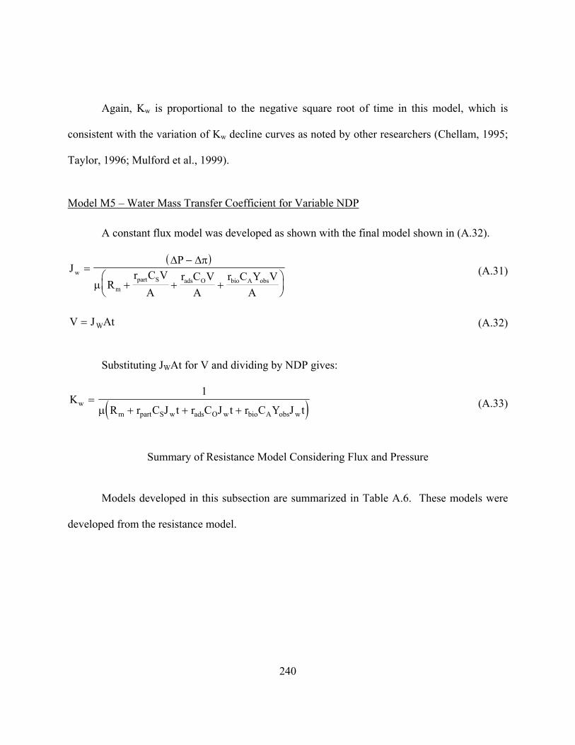
240
Again, Kw is proportional to the negative square root of time in this model, which is
consistent with the variation of Kw decline curves as noted by other researchers (Chellam, 1995;
Taylor, 1996; Mulford et al., 1999).
Model M5 – Water Mass Transfer Coefficient for Variable NDP
A constant flux model was developed as shown with the final model shown in (A.32).
( )J
P
Rr C V
Ar C V
Ar C Y V
A
w
mpart S ads O bio A obs
=−
+ + +⎛⎝⎜
⎞⎠⎟
∆ ∆π
µ (A.31)
t (A.32)
Substituting JWAt for V and dividing by NDP gives:
V J AW=
( )KR r C J t r C J t r C Y J t
wm part S w ads O w bio A obs w
=+ + +
1
µ (A.33)
Summary of Resistance Model Considering Flux and Pressure
Models developed in this subsection are summarized in Table A.6. These models were
developed from the resistance model.
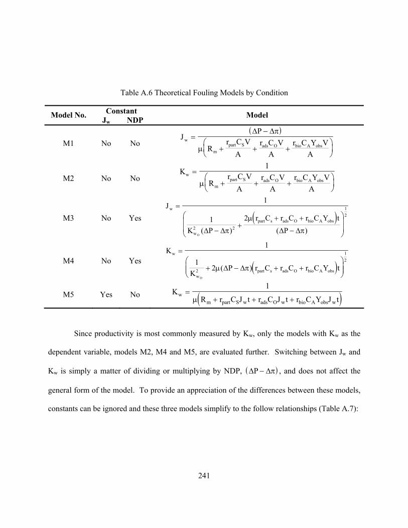
241
Table A.6 Theoretical Fouling Models by Condition
Constant Model No. Jw NDP Model
M1 No No ( )
JP
Rr C V
Ar C V
Ar C Y V
A
w
mpart S ads O bio A obs
=−
+ + +⎛⎝⎜
⎞⎠⎟
∆ ∆π
µ
M2 No No K
Rr C V
Ar C V
Ar C Y V
A
w
mpart S ads O bio A obs
=+ + +
⎛⎝⎜
⎞⎠⎟
1
µ
M3 No Yes ( )J
K Pr C r C r C Y t
P
w
w
part s ads O bio A obs
O
=
−+
+ +
−
⎛
⎝
⎜⎜
⎞
⎠
⎟⎟
1
1 22 2
12
( ) ( )∆ ∆π ∆ ∆π
µ
M4 No Yes ( )K
KP r C r C r C Y t
w
wpart s ads O bio A obs
O
=
+ − + +⎛
⎝⎜⎜
⎞
⎠⎟⎟
1
122
12
µ( )∆ ∆π
( )KR r C J t r C J t r C Y J t
wm part S w ads O w bio A obs w
=+ + +
1
µ M5 Yes No
Since productivity is most commonly measured by Kw, only the models with Kw as the
dependent variable, models M2, M4 and M5, are evaluated further. Switching between Jw and
Kw is simply a matter of dividing or multiplying by NDP, ( )∆ ∆πP − , and does not affect the
general form of the model. To provide an appr odels,
constants can be ignored and these three models simplify to the follow relationships (Table A.7):
eciation of the differences between these m

242
Table A.7 Theoretical Fouling Models – Relationship to Independent Variables
Constant Model No. Jw NDP Proportionality
M2 No No KCVw ∝1
M4 No Yes ( )
KCt
w ∝1
12
KCtw ∝1
M5 Yes No
The original assumption that drove the development of these models was that fouling was
a function of cumulative volume of water produced. Model M2 still is in this form. Kw will be
lower in Model 5 (constant flux) than in Model 4 (constant pressure) over the same period of
operation. This is logical since the flux in Model M4 (constant pressure) is declining with time
and the cumulative volume at time t will be less than with Model M5, which has a constant flux.
For a given period of time, more water will be processed through a system operating at constant
flux than constant pressure, therefore more foulant would be deposited. This would coorespond
to a lower Kw.
The most flexible of the three models is M2, which is valid for varying flux and varying
pressure. Many membrane systems operate at fixed flux or fixed pressure. Over the thousands of
hours of pilot operation conducted as part of this research, flux and/or pressure varied
periodically. Therefore, Model M2 is the best model and is uised for assessment of pilot results .
Models M4 and M5 would be of interest to researchers evaluating controlled conditions of flux
or pressure.

243
MEMBRANE SELECTION STUDY RESULTS
The membrane selection study was conducted to identify nanofiltration membranes that
best meet the water quality objectives of the project. Water quality goals were established prior
to testing and are presented in Table A.8. These water quality goals represent the overall goals
for all systems tested in this project.
Table A.8 Water Quality Goals
Parameter Units Goal Absolutes pH units 7-9 -
temperature degrees C - - alkalinity mg/L as CaCO3 20-100 -
total hardness mg/L as CaCO3 20-100 - turbidity ntu < 0.1 < 0.2
particle counts #/ml < 150 - color cpu 0 < 1 TOC mg/L < 0.5 < 2 Br- µg/L < 0.1 -
UV-254 cm-1 - - iron mg/L < 0.01 < 0.05
manganese mg/L < 0.01 < 0.05 nitrate mg/L < 5 < 10
Silt Density Index units < 1 < 5 SDS-THM µg/L - < 40 SDS-HAA µg/L < 25 < 30 SDS-TOX mg/L < 100 -
The experimental plan developed for the selection study called for flat sheet laboratory-
scale comparison of multiple membrane films. Two separate sets of tests were conducted to
select a composite thin film (CTF) membrane and a cellulose acetate membrane for use at
Tampa. Results are presented in the following sections.

Treatme
membrane experim
reservoir water and were analy
Table A
reservoir and settled w
parameters, designated Set B.
experim
244
Composite Thin Film Results
Reservoir and settled water samples collected from the Hillsborough River Water
nt Plant in September 1996 and were transported to UCF for the composite thin film
ents. An initial set of experiments, designated Set A, were conducted using
zed for a limited group of water quality parameters as shown in
.9. Based on this initial screening, four membranes were selected and retested using
aters, which was analyzed for an expanded group of water quality
In addition, flow and pressure were recorded during the
ents.
Set A Composite Thin Film Results
In September 1996, experiments were conducted using reservoir water and ten composite
thin film (CTF) membrane films. The ten films tested are shown in Table A.10. Results are
presented in Table A.11. Based on these results, four membranes were selected for additional
testing and designated Set B. Selection of the four Set B membranes involved evaluation of the
Set A results as described herein.
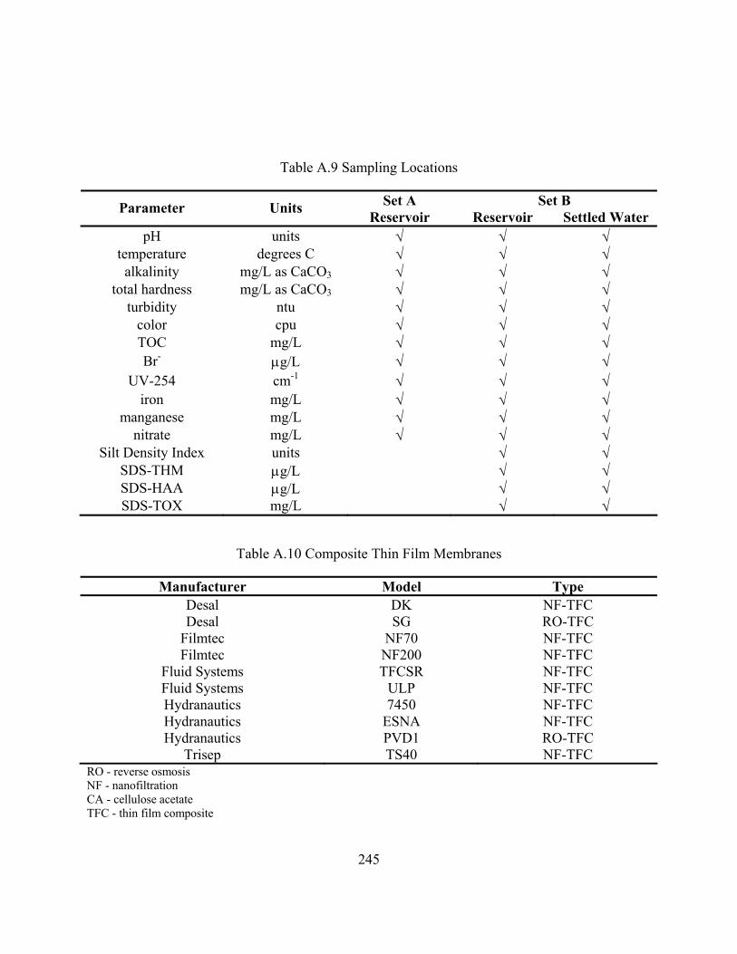
Paramete
temalkalinity
245
Table A.9 Sampling Locations
Set A Set B r Units Reservoir Reservoir Settled Water pH units √ √ √
perature degrees C √ √ √ mg/L as CaCO3 √ √ √
total hardness mg/L as CaCO3 √ √ √ turbidity ntu √ √ √
color cpu √ √ √ TOC mg/L √ √ √ Br- µg/L √ √ √
UV-254 cm-1 √ √ √ iron mg/L √ √ √
manganese mg/L √ √ √ nitrate mg/L √ √ √
Silt Density Index units √ √ SDS-THM µg/L √ √ SDS-HAA µg/L √ √ SDS-TOX mg/L √ √
Table A.10 Composite Thin Film Membranes
Manufacturer Model Type Desal DK NF-TFC Desal SG RO-TFC
Filmtec NF70 NF-TFC Filmtec NF200 NF-TFC
Fluid Systems TFCSR NF-TFC Fluid Systems ULP NF-TFC Hydranautics 7450 NF-TFC Hydranautics ESNA NF-TFC Hydranautics PVD1 RO-TFC
Trisep TS40 NF-TFC RO - reverse osmosis NF - nanofiltration CA - cellulose acetate TFC - thin film composite

Table A.11 Set A Composite Thin Film Results
Press. Kw TH (mg/L) Alk (mg/L) Br UV-254 Color Fe Mn Turbidity TOC Nitrate Membrane
(psi) (gfd/psi) (as CaCO3) (as CaCO3) (mg/L) (cm-1) (cpu) (µg/L) (µg/L) (NTU) (mg/L) (mg/L) Goal 20-100 20-100 < 0.1 - 0 < 10 < 10 < 0.1 < 0.5 < 5
Absolute Goal - - - - < 1 < 50 < 50 < 0.2 < 2.0 < 10 Reservoir 155 112 1.573 0.3831 59 12 6.4 4.4 8.9 1.9
Filmtec NF70 60 0.28 10 14 <0.05 0.0807 2 < 1 <0.05 0.06 1 <0.05 Filmtec NF200 60 0.28 74 26 <0.05 0.088 2 < 1 0.1 0.02 0.9 0.10
Hydra 7450 70 0.25 110 99 <0.05 0.06285 5 < 1 3.5 0.10 2 0.10 Trisep TS40 70 0.24 94 64 0.05 0.03045 3 < 1 2.9 0.02 1 0.10
Fluid Sys TFCSR 70 0.22 53 59 <0.05 0.0287 1 < 1 1.4 0.05 0.5 0.10 Fluid Sys ULP 75 0.22 4 45 <0.05 0.0051 1 < 1 <0.05 0.12 0.2 <0.05
Desal DK 80 0.21 109 94 1.555 0.12905 4 < 1 0.8 0.08 1.6 1.7 Hydra ESNA 80 0.19 15 15 <0.05 0.0227 1 < 1 <0.05 0.02 0.5 <0.05 Hydra PVD1 140 0.12 0 <5 <0.05 0.0077 2 < 1 <0.05 0.11 0.4 4.4*
Desal SG 200 0.06 0 <5 <0.05 0.0075 2 < 1 <0.05 0.15 0.4 <0.05

As shown in Table A.11, only the Desal DK and Hydranautics 7450 produced water of
significantly lesser quality than desired. Four membranes out of the eight eligible membranes
were selected for further evaluation using the following methodology. 1) membranes requiring
lower operating pressure be selected over those requiring higher pressures; and 2) that, all other
factors being equal, each manufacturer have one membrane tested in Set B. The four membranes
selected for Set B analysis were the Fluid Systems ULP, the Filmtec NF200, the Trisep TS40,
and the Hydranautics ESNA.
Set B Composite Thin Film Results
Set B experiments consisted of testing the four selected membranes using both reservoir
and settled waters. These experiments were completed in October 1996 and results are presented
in Table A.12. As shown, the Trisep TS40 was generally a lower rejection membrane and
resulted in higher color, manganese, NPDOC, SDS-THM, and SDS-HAA levels than was
desirable. The Filmtec NF200 produced water with slightly higher than desirable manganese,
SDS-THM and SDS-HAA concentrations. The Fluid Systems ULP and the Hydranautics ESNA
meet all water quality goals and produced a superior water to other membranes tested. Both
membranes were acceptable for evaluation at Tampa. The Hydranautics ESNA was ultimately
selected for Tampa since the cellulose acetate testing (described below) resulted in selection of a
Fluid Systems membrane. This allowed representation of two manufacturers at the Tampa site.

Table A.12 Set B Composite Thin Film Results
Press. Kw TH (mg/L) Alk (mg/L) Br UV-254 Color Fe Mn Turbidity TOC Nitrate Membrane
(psi) (gfd/psi) (as CaCO3) (as CaCO3) (mg/L) (cm-1) (cpu) (µg/L) (µg/L) (NTU) (mg/L) (mg/L) Goal 20-100 20-100 < 0.1 - 0 < 10 < 10 < 0.1 < 0.5 < 5
Absolute Goal - - - - < 1 < 50 < 50 < 0.2 < 2.0 < 10 Reservoir 142 116 na 0.382 58 21 5.7 3 5 na
Filmtec NF200 53 0.34 92 75 na 0.015 1 <1 3 0.1 0.5 na Fluid Sys ULP 90 0.18 1 7 na 0.005 2 <1 <0.05 0.11 0.3 na Trisep TS40 97 0.17 102 64 na 0.047 4 <1 2.6 0.09 1.3 na Hydra ESNA 80 0.23 14 11 na 0.019 1 <1 1 0.02 0.5 na
Settled 146 38 na 0.088 4 <1 255 0.84 3.3 na Filmtec NF200 60 0.30 53 28 na 0.021 2 <1 78 0.01 0.6 na Fluid Sys ULP 70 0.27 1 <5 na 0.005 1 <1 1 0.12 0.3 na Trisep TS40 97 0.18 60 24 na 0.039 2 <1 102 0.04 1 na Hydra ESNA 69 0.24 5 <5 na 0.019 2 <1 9 0.02 0.5 na

250
SDI5 THM HAA TOX Total Pesticides Membrane (units) (µg/L) (µg/L) (µg/L) (µg/L)
Goal < 1 < 30 < 25 < 100 < 0.1 total Absolute Goal < 5 < 40 < 30 - < 0.5 total
Reservoir 194 82 632 < 0.1 Filmtec NF200 32 16 103 na Fluid Sys ULP 7 17 53 na Trisep TS40 93 36 213 na Hydra ESNA 20 29 415 na
Settled 188 106 127 na Filmtec NF200 44 na 107 na Fluid Sys ULP 5 14 38 na Trisep TS40 80 26 197 na Hydra ESNA 33 31 119 na
Cellulose Acetate Results
In addition to a composite thin film membrane, A cellulose acetate was selected as it was
purportedly more resistant to fouling. Four cellulose acetate membranes were tested on raw
water from the Hillsborough River. These were the Hydranautics CAB1, Hydranautics CAB4,
Desal CA/CE and Fluid Systems CALP. Testing occurred in March and April 1997 and results
are presented in Table A.13. Due to time limitations, the cellulose acetate membranes were
analyzed for fewer parameters than the composite thin film membranes. As shown, the Fluid
Systems CALP required the least pressure and was able to meet all water quality goals except
TOC. Given its ability to meet the THM and HAA goals, the Fluid Systems CALP was selected
for pilot testing. Thus, the Fluid Systems CALP and the Hydranautics ESNA were chosen for
evaluation at pilot-scale.

Table A.13 Flat Sheet Testing Results for Cellulose Acetate Membranes
Pressure Kw TDS TH Particle Counts UV-254 TOC Cl2 dose Cl2
residual THM HAA Sample
psi gsfd/psi mg/l mg/l as CaCO3
#/ml (>0.5um) cm-1 mg/L mg/l mg/l µg/l µg/l
Raw 210 206 167,000 0.15 5.9 8 1.5 263 163.6
CA/CE 195 0.072 0 0 1,200 0.0037 0.8 1.5 1.2 8 19.4
CAB1 170 0.102 10 6 4,600 0.0045 1 1.5 1.2 10 18.2
CALP 100 0.173 40 35 2,200 0.0091 1 1.5 1 12 22.7
CAB4 170 0.083 10 6 3,900 0.0063 0.6 1.5 1.1 9 10.1 Desal CACE Hydranautics CAB1 and CAB4 Fluid Systems CALP
252
PILOT STUDY RESULTS
Pilot testing of the integrated membrane systems began in May 1997 and lasted through
October 1998. This section presents an overview of the nanofilter operational data collected
during that time. In addition, cleaning cycles are estimated using linear regression of Kw with
time, as this is the most common method of assessing fouling rates. Matching the operational
results to the resistance models presented above is presented later in this document. Finally,
although the nanofilters were operated in conjunction with a pretreatment system, these systems
are only discussed in relation to their impact on nanofilter performance.
As described in the sections below, three nanofilters were ultimately tested at the Tampa
site. The Fluid Systems CALP and the Hydranautics ESNA were chosen as a result of the
Membrane Selection Study. During the course of testing, it was determined that the ESNA
membrane was not suitable for treating the Hillsborough River, as discussed later in this Chapter.
The Hydranautics LFC1 nanofilter was recommended by the manufacturer and replaced the
ESNA. The characteristics of these three nanofilters, as reported by the manufacturers, are
presented in Table A.14.
All productivity data presented in this dissertation have been temperature corrected to 20°
Celsius. All projections of chemical cleaning cycles are based on a linear regression of water
mass transfer coefficient with time, the initial Kw, and a 15 percent decline in productivity. The
linear regression provides a slope (dKw/dt) as shown in Equation (A.34) is the most common
model in the membrane industry and is used here to present the pilot results. Following this

253
presentation, the multivariate nonlinear model developed as part of this dissertation (Model M2)
will be compared to the linear model and assessed for its applicability to these data.
tdt
dKKK WWw O
×±= (A.34)
Where
Kw = water mass transfer coefficient
= initial water mass transfer coefficient
dKw/dt = rate of Kw decline over time, or slope
t = operational time
In this section, each linear regression includes calculation of the 95% confidence limits
for the slope. Based on these limits, a range was defined for the cleaning cycle. Specifically, the
lower limit for the slope is a conservative characterization of the worst-case (shortest) cleaning
cycle. The upper limit for the slope is a best-case (longest) estimate of the cleaning cycle. This
assessment is especially important since experiments were no more than 2-weeks in length,
which resulted in relatively more data variability. This duration may not be sufficient for
prediction of very shallow declines in Kw with time that are associated with minor fouling and
long cleaning cycles. However, the 95% confidence level limits for Kw decline provide a range
for the estimated cleaning cycle and is a convenient means of conveying the variability and
limitations of the data.
KWO
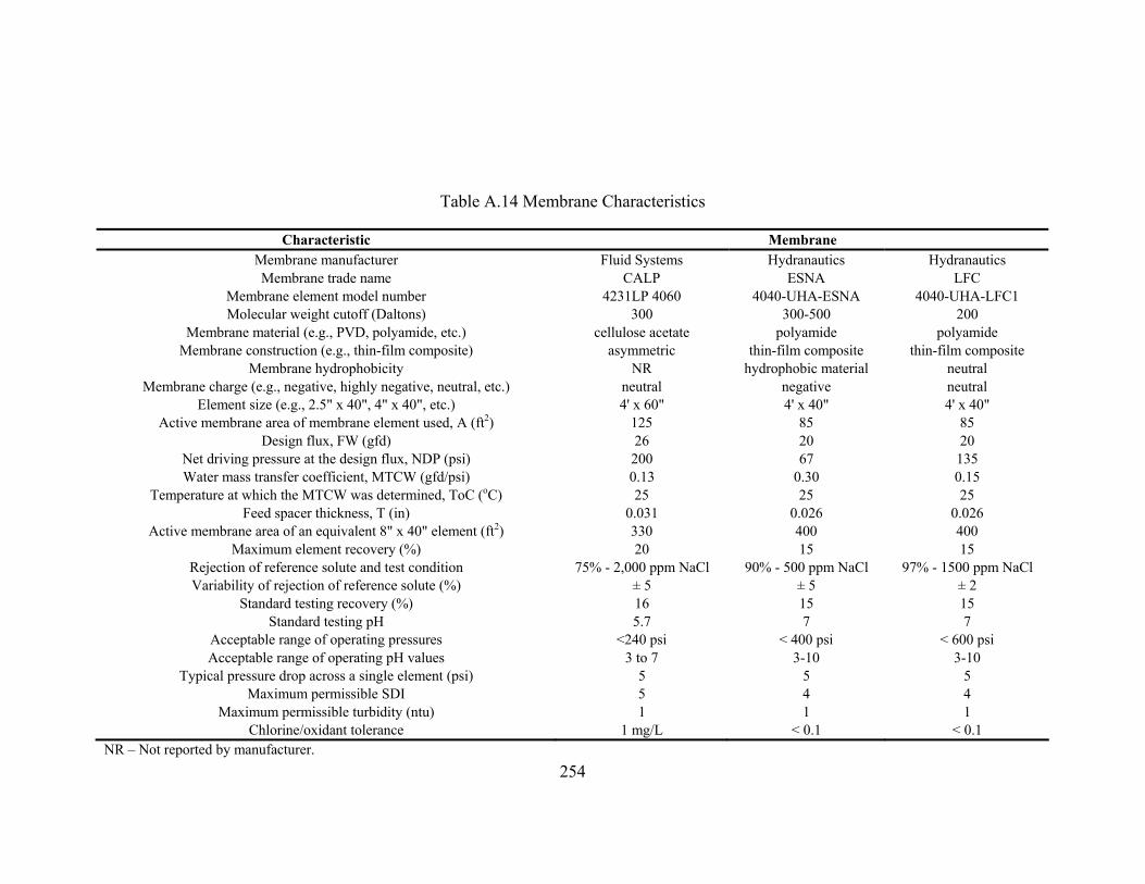
254
Table A.14 Membrane Characteristics
Characteristic Membrane Membrane manufacturer Fluid Systems Hydranautics Hydranautics Membrane trade name CALP ESNA LFC
Membrane element model number 4231LP 4060 4040-UHA-ESNA 4040-UHA-LFMolecular weight cutoff (Daltons) 300 300-500 200
Membrane material (e.g., PVD, polyamide, etc.) cellulose acetate polyamide polyamide Membrane construction (e.g., thin-film composite) asymmetric thin-film composite thin-film com
Membrane hydrophobicity NR hydrophobic material neutral Membrane charge (e.g., negative, highly negative, neutral, etc.) neutral negative neutral
Element size (e.g., 2.5" x 40", 4" x 40", etc.) 4' x 60" 4' x 40" 4' x 40" Active membrane area of membrane element used, A (ft2) 125 85 85
Design flux, FW (gfd) 26 20 20 Net driving pressure at the design flux, NDP (psi) 200 67 135 Water mass transfer coefficient, MTCW (gfd/psi) 0.13 0.30 0.15
Temperature at which the MTCW was determined, ToC (oC) 25 25 25 Feed spacer thickness, T (in) 0.031 0.026 0.026
Active membrane area of an equivalent 8" x 40" element (ft2) 330 400 400 Maximum element recovery (%) 20 15 15
Rejection of reference solute and test condition 75% - 2,000 ppm NaCl 90% - 500 ppm NaCl 97% - 1500 ppm NaCl Variability of rejection of reference solute (%) ± 5 ± 5 ± 2
Standard testing recovery (%) 16 15 15 Standard testing pH 5.7 7 7
Acceptable range of operating pressures <240 psi < 400 psi < 600 psi Acceptable range of operating pH values 3 to 7 3-10 3-10
Typical pressure drop across a single element (psi) 5 5 5 Maximum permissible SDI 5 4 4
Maximum permissible turbidity (ntu) 1 1 1 Chlorine/oxidant tolerance 1 mg/L < 0.1 < 0.1
C1
posite
NR – Not reported by manufacturer.

255
Hydranautics ESNA Nanofilter
The Hydranautics ESNA nanofilter was evaluated using CSF and UF pretreated feed
waters. Nanofilter productivity and water quality testing results are presented in the following
sections.
Hydranautics ESNA Productivity
The CSF-ESNA and UF-ESNA process trains used different sets of ESNA elements in
two different NF pilot units. The CSF-ESNA system used nine ESNA 4-inch diameter x 40-inch
long elements in a 2-1 array system. The UF-ESNA system used one ESNA 4-inch diameter x
40-inch long element. Therefore separate productivity plots are provided by system. Turbidity
and TOC in the nanofilter feed is presented as these are primary factors for particle fouling and
organic adsorption and biogrowth, respectively. Later experiments included assessment of
biogrowth via heterotrophic plate counts (HPCs), which was not collected for the ESNA
experiments.
Coagulation, Sedimentation, Filtration Pretreatment
CSF-ESNA productivity plots of flux, recovery, feed-side differential pressure, and water
mass transfer coefficient are presented in Figure A.5, Figure A.6, Figure A.7, and Figure A.8,
respectively. As shown, flux was set at 7 or 14 gfd. Recovery was set at 65 or 85 percent. The
first experiment evaluated a flux and recovery of 7 gfd and 65 percent, respectively. At
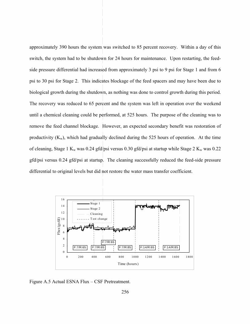
256
approximately 390 hours the system was switched to 85 percent recovery. Within a day of this
switch, the system had to be shutdown for 24 hours for maintenance. Upon restarting, the feed-
side pressure differential had increased from approximately 3 psi to 9 psi for Stage 1 and from 6
psi to 30 psi for Stage 2. This indicates blockage of the feed spacers and may have been due to
biological growth during the shutdown, as nothing was done to control growth during this period.
The recovery was reduced to 65 percent and the system was left in operation over the weekend
until a chemical cleaning could be performed, at 525 hours. The purpose of the cleaning was to
remove the feed channel blockage. However, an expected secondary benefit was restoration of
productivity (Kw), which had gradually declined during the 525 hours of operation. At the time
of cleaning, Stage 1 Kw was 0.24 gfd/psi versus 0.30 gfd/psi at startup while Stage 2 Kw was 0.22
gfd/psi versus 0.24 gfd/psi at startup. The cleaning successfully reduced the feed-side pressure
differential to original levels but did not restore the water mass transfer coefficient.
0
2
4
6
8
10
12
14
16
0 200 400 600 800 1000 1200 1400 1600 1800
Time (hours )
Flux
(gsf
d)
St age 1
St age 2
Clean ingT est change
F:7/R:65 F:7/R:65
F:7/R:65
F:7/R:85 F:14/R:65 F:14/R:85
Figure A.5 Actual ESNA Flux – CSF Pretreatment.

257
0
10
20
30
40
50
60
70
80
90
100
0 200 400 600 800 1000 1200 1400 1600 1800Time (hours)
Rec
over
y (%
)
S ys te m R e c o ve ry
C le a ning
Te s t c ha nge
F:7/R:65 F:7/R:65
F:7/R:65
F:7/R:85 F:14/R:65 F:14/R:85
Figure A.6 ESNA Recovery – CSF Pretreatment.
0
10
20
30
40
50
60
0 200 400 600 800 1000 1200 1
Time (hours)
Feed
-Sid
e P
(psi
)
400 1600 1800
S ta ge 1 S ta ge 2
C le a n ing T e s t c ha nge
F:7/R:65 F:7/R:65
F:7/R:65
F:7/R:85 F:14/R:65 F:14/R:85
ent. Figure A.7 Actual ESNA Feed-Side Differential Pressure – CSF Pretreatm
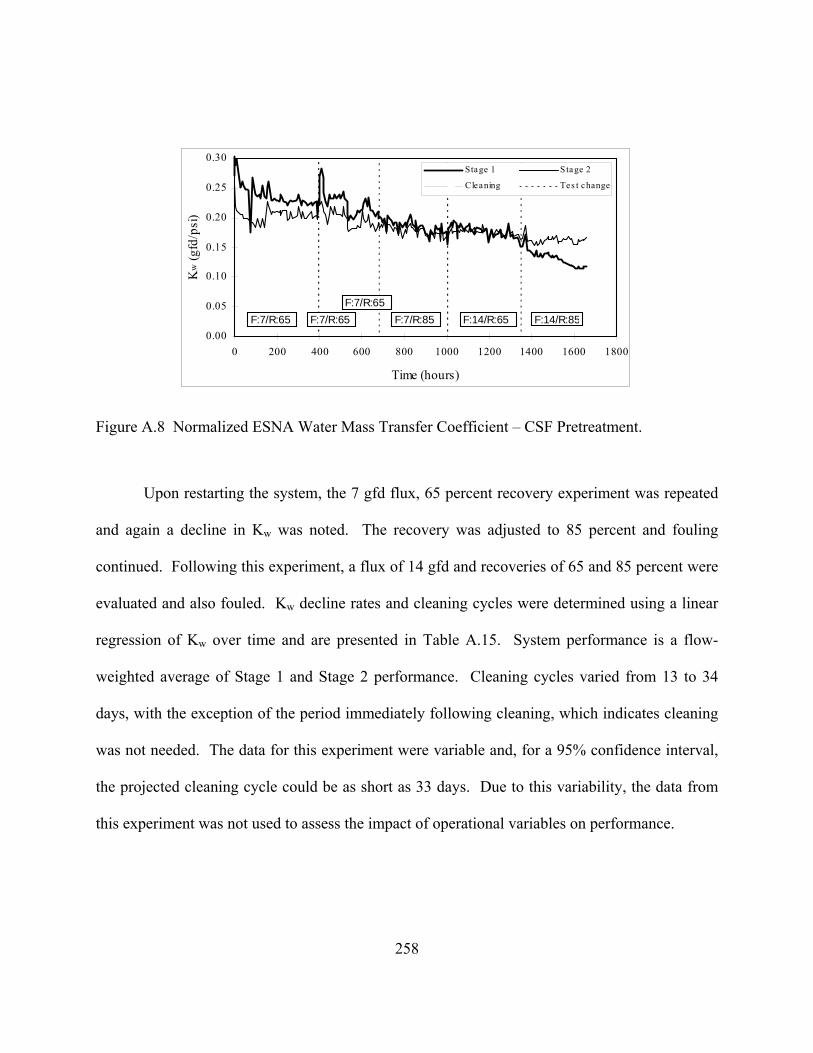
0.00
0.05
0.10
0.15
0.20
0.25
0.30
0 200 400 600 800 1000 1200 1400 1600 1800
Time (hours)
Kw
(gfd
/psi
)
S tage 1 Stage 2
Cleaning Tes t change
F:7/R:65 F:7/R:65F:7/R:65
F:7/R:85 F:14/R:65 F:14/R:85
Figure A.8 Normalized ESNA Water Mass Transfer Coefficient – CSF Pretreatment.
Upon restarting the system, the 7 gfd flux, 65 percent recovery experiment was repeated
and again a decline in Kw was noted. The recovery was adjusted to 85 percent and fouling
continued. Following this experiment, a flux of 14 gfd and recoveries of 65 and 85 percent were
evaluated and also fouled. Kw decline rates and cleaning cycles were determined using a linear
regression of Kw over time and are presented in Table A.15. System performance is a flow-
weighted average of Stage 1 and Stage 2 performance. Cleaning cycles varied from 13 to 34
days, with the exception of the period immediately following cleaning, which indicates cleaning
was not needed. The data for this experiment were variable and, for a 95% confidence interval,
the projected cleaning cycle could be as short as 33 days. Due to this variability, the data from
this experiment was not used to assess the impact of operational variables on performance.
258
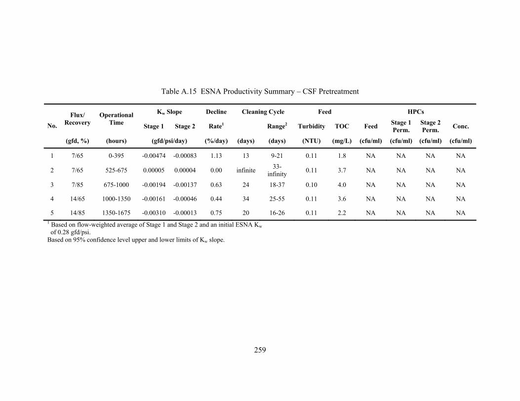
259
Table A.15 ESNA Productivity Summary – CSF Pretreatment
Kw Slope Decline Cleaning Cycle Feed HPCs Flux/ Recovery
Operational Time Stage 1 Stage 2 Rate1 Range2 Turbidity TOC Feed Stage 1
Perm. Stage 2 Perm. Conc. No.
(gfd, %) (hours) (gfd/psi/day) (%/day) (days) (days) (NTU) (mg/L) (cfu/ml) (cfu/ml) (cfu/ml) (cfu/ml)
1 7/65 0-395 -0.00474 -0.00083 1.13 13 9-21 0.11 1.8 NA NA NA NA
2 7/65 525-675 0.00005 0.00004 0.00 infinite 33-infinity 0.11 3.7 NA NA NA NA
3 7/85 675-1000 -0.00194 -0.00137 0.63 24 18-37 0.10 4.0 NA NA NA NA
4 14/65 1000-1350 -0.00161 -0.00046 0.44 34 25-55 0.11 3.6 NA NA NA NA
5 14/85 1350-1675 -0.00310 -0.00013 0.75 20 16-26 0.11 2.2 NA NA NA NA 1 Based on flow-weighted average of Stage 1 and Stage 2 and an initial ESNA Kw of 0.28 gfd/psi. Based on 95% confidence level upper and lower limits of Kw slope.
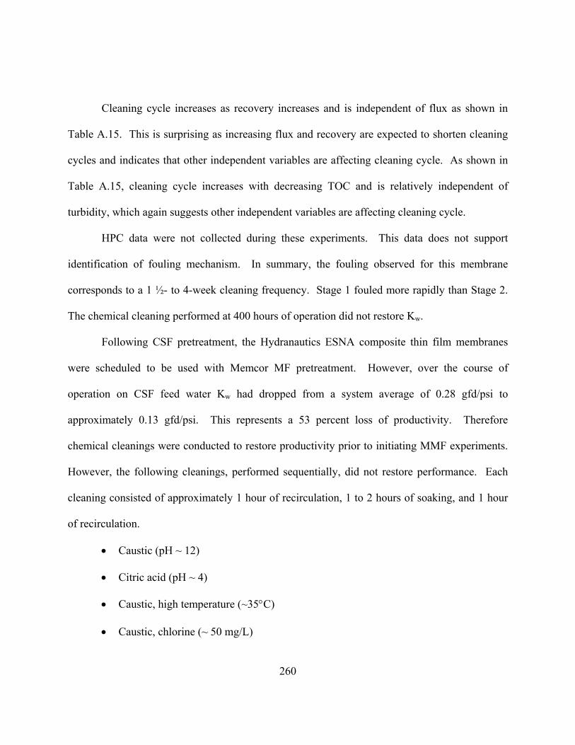
260
Cleaning cycle increases as recovery increases and is independent of flux as shown in
Table A.15. This is surprising as increasing flux and recovery are expected to shorten cleaning
cycles and indicates that other independent variables are affecting cleaning cycle. As shown in
Table A.15, cleaning cycle increases with decreasing TOC and is relatively independent of
turbidity, which again suggests other independent variables are affecting cleaning cycle.
HPC data were not collected during these experiments. This data does not support
identification of fouling mechanism. In summary, the fouling observed for this membrane
corresponds to a 1 ½- to 4-week cleaning frequency. Stage 1 fouled more rapidly than Stage 2.
The chemical cleaning performed at 400 hours of operation did not restore Kw.
Following CSF pretreatment, the Hydranautics ESNA composite thin film membranes
were scheduled to be used with Memcor MF pretreatment. However, over the course of
operation on CSF feed water Kw had dropped from a system average of 0.28 gfd/psi to
approximately 0.13 gfd/psi. This represents a 53 percent loss of productivity. Therefore
chemical cleanings were conducted to restore productivity prior to initiating MMF experiments.
However, the following cleanings, performed sequentially, did not restore performance. Each
cleaning consisted of approximately 1 hour of recirculation, 1 to 2 hours of soaking, and 1 hour
of recirculation.
• Caustic (pH ~ 12)
• Citric acid (pH ~ 4)
• Caustic, high temperature (~35°C)
• Caustic, chlorine (~ 50 mg/L)

261
• Caustic, high temperature, EDTA (~ 0.25%), Biz detergent (~ 0.25%)
• Citric acid, high temperature
• Citric acid
• Caustic, chlorine, EDTA
• Caustic, chlorine, EDTA
• Caustic, EDTA, overnight soak
• Caustic, EDTA, chlorine
These cleanings were coordinated with the manufacturer and represented the most
promising and most aggressive solutions known to be available. Following this extensive
cleaning effort, it was determined that the ESNA membrane, for this site, could not be cleaned.
Regardless of the rate of productivity decline during the course of normal operation, the ESNA is
not a viable membrane since ESNA fouling is permanent. The ESNA membrane was replaced
by the Hydranautics LFC1.
UF Pretreatment
ConcurrConcurrent to the CSF-ENSA experiments, UF-ESNA performance was
evaluated using the single element nanofiltration system and the Aquasource ultrafiltration unit.
Nanofilter productivity plots for flux, recovery, feed-side differential pressure, and water mass
transfer coefficient are presented in Figure A.9, Figure A.10, Figure A.11 and Figure A.12,
respectively. Flux was set at 7 or 14 gfd. Recovery was set at 65 or 85 percent. As shown in
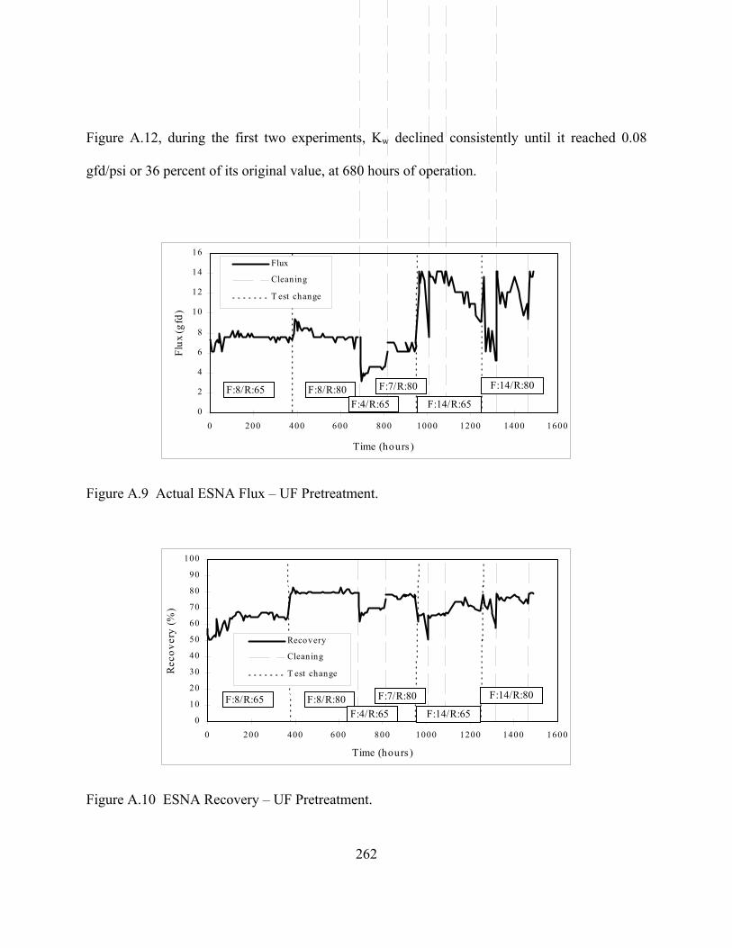
262
Figure A.12, during the first two experiments, Kw declined consistently until it reached 0.08
gfd/psi or 36 percent of its original value, at 680 hours of operation.
0
2
4
6
8
10
12
14
16
0 200 400 600 800 1000 1200 1400 1600
Time (hours )
Flux
(gfd
)
Flux
Cleaning
T est change
F:8/R:65 F:8/R:80F:4/R:65
F:7/R:80
F:14/R:65
F:14/R:80
Figure A.9 Actual ESNA Flux – UF Pretreatment.
0
10
20
30
40
50
60
70
80
0 200 400 600 800 1000 1200 1400 1600
Time (hours )
Rec
over
y (%
)
90
100
Recovery
Cleaning
T est change
F:8/R:65 F:8/R:80F:4/R:65
F:7/R:80
F:14/R:65
F:14/R:80
Figure A.10 ESNA Recovery – UF Pretreatment.
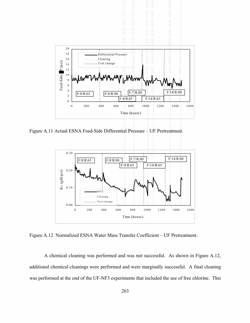
Figur
263
0
2
4
6
8
1 0
1 2
1 4
1 6
1 8
2 0
0 200 400 600 800 1000 1200 1400 1600
Time (hours )
Feed
-Sid
e P
(psi
)
Different ial P ressureCleaningT est change
F:8/R:65 F:8/R:80F:4/R:65
F:7/R:80
F:14/R:65
F:14/R:80
ntial Pressure – UF Pretreatme A.11 Actual ESNA Feed-Side Differe ent.
0.00
0.10
0.20
0.30
0 200 400 600 800 1000 1200
Time (hours )
Kw
(gfd
/psi
)
1400 1600
M T C
C le a ning
T e s t c ha nge
F:8/R:65 F:8/R:80F:4/R:65
F:7/R:80
F:14/R:65
F:14/R:80
cient – UF Pretreatment.
t successful. As shown in Figure A.12,
successful. A final cleaning
Figure A.12 Normalized ESNA Water Mass Transfer Coeffi
A chemical cleaning was performed and was no
additional chemical cleanings were performed and were marginally
was performed at the end of the UF-NF3 experiments that included the use of free chlorine. This
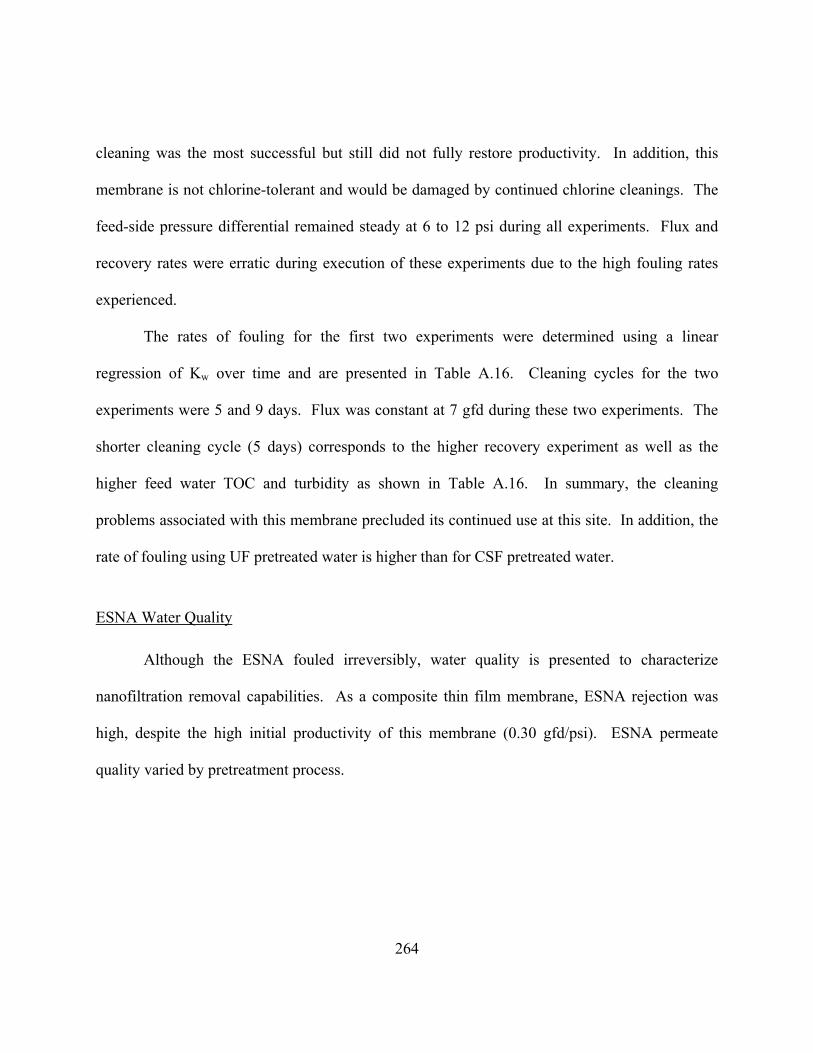
264
cleaning was the most successful but still did not fully restore productivity. In addition, this
membrane is not chlorine-tolerant and would be damaged by continued chlorine cleanings. The
feed-side pressure differential remained steady at 6 to 12 psi during all experiments. Flux and
recovery rates were erratic during execution of these experiments due to the high fouling rates
experienced.
The rates of fouling for the first two experiments were determined using a linear
regression of Kw over time and are presented in Table A.16. Cleaning cycles for the two
experiments were 5 and 9 days. Flux was constant at 7 gfd during these two experiments. The
shorter cleaning cycle (5 days) corresponds to the higher recovery experiment as well as the
higher feed water TOC and turbidity as shown in Table A.16. In summary, the cleaning
problems associated with this membrane precluded its continued use at this site. In addition, the
rate of fouling using UF pretreated water is higher than for CSF pretreated water.
ESNA Water Quality
Although the ESNA fouled irreversibly, water quality is presented to characterize
nanofiltration removal capabilities. As a composite thin film membrane, ESNA rejection was
high, despite the high initial productivity of this membrane (0.30 gfd/psi). ESNA permeate
quality varied by pretreatment process.

265
Table A.16 ESNA Productivity Summary – UF Pretreatment
Decline Cleaning Cycle Feed HPCs No. Flux/
Recovery Operational
Time Kw Slope Rate1 Range2 Turbidity TOC Feed Perm. Conc.
(gfd, %) (hours) (gfd/psi/day) (%/day) (days) (days) (NTU) (mg/L) (cfu/ml) (cfu/ml) (cfu/ml)
1 7/65 0-365 -0.00373 1.69 9 7-11 0.12 17.4 NA NA NA
2 7/85 365-695 -0.00600 2.73 5 5-6 0.14 25.4 NA NA NA
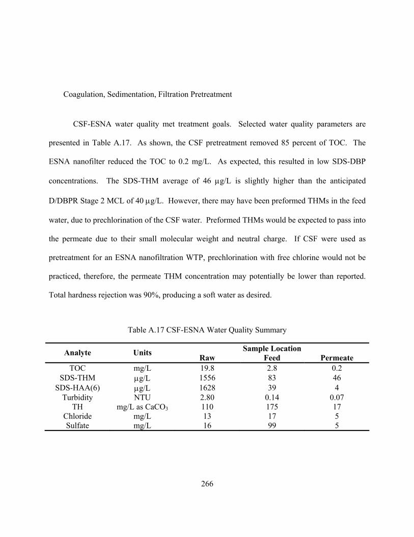
266
Coagulation, Sedimentation, Filtration Pretreatment
CSF-ESNA water quality met treatment goals. Selected water quality parameters are
presented in Table A.17. As shown, the CSF pretreatment removed 85 percent of TOC. The
ESNA nanofilter reduced the TOC to 0.2 mg/L. As expected, this resulted in low SDS-DBP
concentrations. The SDS-THM average of 46 µg/L is slightly higher than the anticipated
D/DBPR Stage 2 MCL of 40 µg/L. However, there may have been preformed THMs in the feed
water, due to prechlorination of the CSF water. Preformed THMs would be expected to pass into
the permeate due to their small molecular weight and neutral charge. If CSF were used as
pretreatment for an ESNA nanofiltration WTP, prechlorination with free chlorine would not be
practiced, therefore, the permeate THM concentration may potentially be lower than reported.
Total hardness rejection was 90%, producing a soft water as desired.
Table A.17 CSF-ESNA Water Quality Summary
Sample Location Analyte Units Raw Feed Permeate TOC mg/L 19.8 2.8 0.2
SDS-THM µg/L 1556 83 46 SDS-HAA(6) µg/L 1628 39 4
Turbidity NTU 2.80 0.14 0.07 TH mg/L as CaCO3 110 175 17
Chloride mg/L 13 17 5 Sulfate mg/L 16 99 5

267
UF Pretreatment
Selected water quality UF-ESNA parameters are presented in Table A.18. As shown, the
UF pretreatment removed no TOC, as expected from a size-exclusion process. The ESNA
nanofilter reduced the 20.8 mg/L TOC feed to 0.5 mg/L, or 97% rejection. SDS-DBP
concentrations were lower for the UF-ESNA system than the CSF-ESNA system; less than 12
µg/L for THMs and HAAs. These levels will meet the anticipated D/DBPR Stage 2 MCLs of 40
and 30 µg/L for THMs and HAAs, respectively. Total hardness rejection was 94%, producing a
soft water as desired.
Table A.18 UF-ESNA Water Quality Summary
Sample Location Analyte Units Raw Feed Permeate TOC mg/L 20.7 20.8 0.5
SDS-THM µg/L 1556 1479 12 SDS-HAA(6) µg/L 1628 1721 6
Turbidity NTU 2.80 0.14 0.08 TH mg/L as CaCO3 110 100 7
Chloride mg/L 13 12 2 Sulfate mg/L 16 13 1
Hydranautics LFC1 Nanofilter
The LFC1 nanofilter was evaluated using MMF, ZMF, CSF, and C/MMF pretreated feed
waters. Productivity and water quality results are presented in the following sections.

268
LFC1 Productivity
The LFC1 was tested using four advanced pretreatment processes. The sequence of
testing was as follows: MMF, ZMF, CSF, ZMF, C/MMF, MMF. As shown, MMF and ZMF
were tested twice. Operational results for flux, recovery, feed-side differential pressure, and
water mass transfer coefficient are presented in Figure A.13, Figure A.14, Figure A.15 and
Figure A.15, respectively. Results are discussed in the chronological order in which
pretreatment processes were evaluated.
0
2
4
6
8
10
12
14
16
18
0 1000 2000 3000 4000 5000Time (hours)
Flux
(gf
d)
Stage 1 Flux Stage 2 FluxCleaning Tes t Change
Z M FCSFZ M F C/M M F M M FM M F
7/8514 /657/65
14/857 /65 7 /85 14 /75
14 /857 /65 14 /85 7 /65 14 /85
7 /6514 /85
14/85
14 /85 14 /85
Figure A.13 Actual LFC1 Flux.
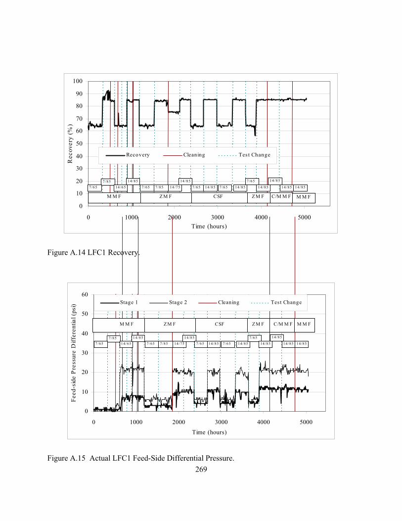
0
10
20
30
40
50
60
70
80
90
100
0 1000 2000 3000 4000 5000Time (hours)
Rec
over
y (%
)
Recovery Cleaning Tes t Change
Z M FCSFZ M F C/M M F M M FM M F
7/8514/657 /65
14/857/65 7/85 14/75
14/857/65 14 /85 7 /65 14/85
7/6514 /85
14/85
14/85 14 /85
Figure A.14 LFC1 Recovery.
0
10
20
30
40
50
0 1000 2000 3000 4000 5000Time (hours)
Feed
-sid
e P
ress
ure
Diff
eren
tial (
psi)
60Stage 1 Stage 2 Cleaning Tes t Change
M M F Z M FCSFZ M F C/M M F M M F
7/8514/657 /65
14/857/65 7/85 14/75
14/857/65 14/85 7/65 14/85
7/6514/85
14 /85
14/85 14/85
Figure A.15 Actual LFC1 Feed-Side Differential Pressure. 269

270
0.00
0.05
0 1000 2000 3000Time (hours)
0.10
0.15
0.20
0.25
0.30
4000 5000
Kw
(gf
d/ps
i)
Stage 1 Kw Stage 2 KwCleaning T est Change
M M F Z M FCSFZ M F C/M M F M M F
7/8514 /657 /65
14 /857 /65 7 /85 14 /75
14 /857 /65 14 /85 7 /65 14 /85
7/6514 /85
14 /85
14 /85 14 /85
ilter during two periods, for nine
experim d and 65%, respectively. This and
ore than a 15 day cleaning
tion (Table A.19). At this
Biological growth was possibley the primary
e waters are highly. Upon consultation with the
ma is capable of withstanding monochloramine, a
oramine injection system was
Figure A.16 Normalized LFC1 Water Mass Transfer Coefficient.
Memcor Microfiltration Pretreatment
MMF pretreatment was tested with the LFC1 nanof
ents. Flux and recovery were initially set at 7 gf
subsequent experiments incurred severe fouling, resulting in no m
cycle for the first seven experiments, through 1,025 hours of opera
point, continued use of the LFC1 was in doubt.
cause of fouling as biocide was used, and surfac
nufacturer, it was determined that the LFC1
disinfectant capable of controlling biological growth. A monochl

271
installed and initiated for the next experiment, at 1,025 hours of operation. Flux and recovery
were set at 14 gfd and 85%, respectively, to replicate the previous experiment. Fouling
mechanism related water quality results are shown in Table A.19. As shown in Table A.19,
fouling was reduced by a factor of 2. As shown in Figure A.16, Kw decline was reduced from
6.4% per day to 3.2% per day. However, the average feed water TOC had dropped from 17.2
mg/L to 6.1 mg/L for the experiment with monochloramine. Therefore, the improvement could
be attributed to the monochloramine or the reduction in TOC. In addition, a decline rate of 3.2%
per day still only represents a 5-day cleaning cycle. These results suggest that the
monochloramine dose of 0.9 mg/L was not adequate for control of biological growth, that
another fouling mechanism was responsible for the observed productivity decline, or both. Thus,
a third replicate experiment was performed at 4,725 hours of operation, using an average
monochloramine dose of 4.9 mg/L. In addition, HPC measurements were taken to ensure control
of biological growth. As shown, HPCs were effectively controlled with monochloramine, TOC
was high (19.1 mg/L) and the estimated cleaning cycle was 5 days, indicating a continued issue
with fouling. These results point to a mechanism other than biogrowth, such as organic
adsorption or particle fouling. An additional possibility is intolerance to monochloramine,
resulting in breakdown and degradation of the membrane film. The effects of flux and recovery
on cleaning cycle in the MMF-LCF 1 IMS are shown in Table A.19, which indicates cleaning
cycle decreases as recovery increases and is independent of flux for the conditions of this work.
The effects of TOC and turbidity on cleaning cycle in the MMF-LCF 1 IMS are shown in Table
A.19, which indicates cleaning cycle increases as as TOC increases and is relatively independent
of turbidity for the conditions of this work.
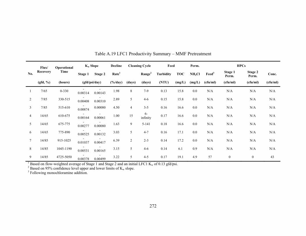
Table A.19 LFC1 Productivity Summary – MMF Pretreatment
Kw Slope Decline Cleaning Cycle Feed Perm. HPCs Flux/ Recovery
Operational Time
Stage 1 Stage 2 Rate1 Range2 Turbidity TOC NH2Cl Feed3 Stage 1 Perm.
Stage 2 Perm. Conc. No.
(gfd, %) (hours) (gfd/psi/day) (%/day) (days) (days) (NTU) (mg/L) (mg/L) (cfu/ml) (cfu/ml) (cfu/ml) (cfu/ml)
1 7/65 0-330 -0.00314
-0.00143 1.98 8 7-9 0.13 15.8 0.0 N/A N/A N/A N/A
2 7/85 330-515 -0.00408
-0.00310 2.89 5 4-6 0.15 15.8 0.0 N/A N/A N/A N/A
3 7/85 515-610 -0.00874 0.00080 4.50 4 3-5 0.16 16.6 0.0 N/A N/A N/A N/A
4 14/65 610-675 -0.00164
-0.00061 1.00 15 6-
infinity 0.17 16.6 0.0 N/A N/A N/A N/A
5 14/65 675-775 -0.00277
-0.00080 1.63 9 5-141 0.18 16.6 0.0 N/A N/A N/A N/A
6 14/65 775-890 -0.00525
-0.00132 3.03 5 4-7 0.16 17.1 0.0 N/A N/A N/A N/A
7 14/85 915-1025 -0.01037
-0.00417 6.39 2 2-3 0.14 17.2 0.0 N/A N/A N/A N/A
8 14/85 1045-1190 -0.00531
-0.00165 3.15 5 4-6 0.14 6.1 0.9 N/A N/A N/A N/A
9 14/85 4725-5050 -0.00378
-0.00499 3.22 5 4-5 0.17 19.1 4.9 57 0 0 43
1 Based on flow-weighted average of Stage 1 and Stage 2 and an initial LFC1 Kw of 0.13 gfd/psi. 2 Based on 95% confidence level upper and lower limits of Kw slope. 3 Following monochloramine addition.
272
273
Zenon Microfiltration Pretreatment
ZMF pretreatment was tested on two occasions with the LFC1 nanofilter in six
experiments. During the first four experiments, monochloramine was applied for control of
biological growth. Fouling and water quality results are presented in Table A.20. As shown, all
experiments with recovery of 65 or 75% (No. 1, 3 and 5) resulted in no observed fouling. The
three experiments at 85% recovery resulted in cleaning cycles ranging from 3 to 21 days.
Permeate HPCs were high for two of the three 85% recovery experiments (No. 1 and 3),
suggesting permeate-side biological growth. It is possible that growth occurring on the permeate
side of a membrane could result in resistance to flow, as is expected for feed-side growth.
Though TOC levels are low in nanofilter permeate, it is possible that small molecular weight
assimilable organic carbon (AOC) could pass through to the permeate and provide a source of
substrate for microbiological growth.
Fouling does not appear related to feed water TOC, as experiment No. 4 resulted in only
a 5 day cleaning cycle yet had the lowest TOC of the six experiments (3.8 mg/L). For
comparison, experiment No. 5 had an average TOC of 16.7 mg/L and resulted in no fouling.

Table A.20 LFC1 Productivity Summary – ZMF Pretreatment
Kw Slope Decline Cleaning Cycle Feed Perm. HPCs Flux/
Recovery Operational
Time Stage 1 Stage 2 Rate1 Range2 Turbidity TOC NH2Cl Feed3 Stage 1
Perm.
Stage 2
Perm. Conc. No.
(gfd, %) (hours) (gfd/psi/day) (%/day) (days) (days) (NTU) (mg/L) (mg/L) (cfu/ml) (cfu/ml) (cfu/ml) (cfu/ml)
1 7/65 1190-1525 0.00096 0.00052 0.00 ∞ Infinity 0.15 10.2 0.9 39,000 1,000 519 6,000
2 7/85 1525-1850 -0.00133
-0.00011 0.71 21 14-47 0.19 9.9 0.5 73,000 341,000 318,000 44,000
3 14/75 1850-2115 0.00192 0.00096 0.00 ∞ Infinity 0.16 4.6 0.6 na na na na
4 14/85 2115-2360 -0.00192
-0.00862 3.19 5 4-6 0.16 3.8 2.2 6,400 <100 10,700 1,650
5 7/65 3640-3890 0.00225 0.00157 0 infinite Infinity 0.15 16.7 0.0 37,050 1,413 1,540 90,200
6 14/85 3890-4145 -0.00536
-0.00630 4.4 3 3-4 0.13 18.0 0.0 6,940 603 1,900 10,675
1 Based on flow-weighted average of Stage 1 and Stage 2 and an initial LFC1 Kw of 0.13 gfd/psi. 2 Based on 95% confidence level upper and lower limits of Kw slope. 3 Following monochloramine addition.
274

275
Finally, monochloramine did not appear to control biogrowth, as evidenced by higher
permeate HPC levels in experiments No. 2 and 4 despite residuals of 0.5 and 2.2 mg/L,
respectively. The effects of flux and recovery, and TOC and turbidity on cleaning cycle are
shown in Table A.20. The observed trends are the same as previously shown on other IMSs.
Cleaning cycle increases as recovery and TOC increases, is independent of flux, is relatively of
turbidity. Although repetitive, the relationship between cleaning cycle and TOC or recovery is
counter institutive and indicates other factors are affecting cleaning cycle.
Coagulation, Sedimentation, Filtration Pretreatment
CSF-LFC1 testing was performed with and without monochloramine addition for a total
of four experiments and as shown in Table A.21. As shown in Table A.21 below, the first two
experiments did not include monochloramine addition and resulted in no observed fouling at 7
gfd flux and 65% recovery versus a 20 day estimated cleaning cycle at 14 gfd flux and 85%
recovery. During this second experiment, HPC counts were high in Stage 1 permeate and in the
concentrate, suggesting biological growth was occurring. These results can be compared to the
third and fourth experiments, in which monochloramine was added. A ninety-nine day cleaning
cycle was estimated for the 7 gfd flux, 65% recovery experiment. No fouling was observed for
the 14 gfd flux, 85% recovery experiment. As shown in Table A.21, there are fewer data points
but the effects of flux, recovery, TOC and turbidity on cleaning cycle are not different than has
been previously shown.
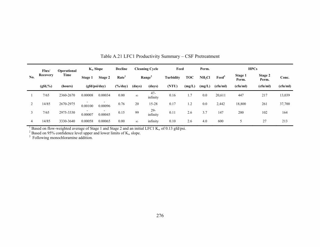
Table A.21 LFC1 Productivity Summary – CSF Pretreatment
Kw Slope Decline Cleaning Cycle Feed Perm. HPCs Flux/ Recovery
Operational Time
Stage 1 Stage 2 Rate1 Range2 Turbidity TOC NH2Cl Feed3 Stage 1 Perm.
Stage 2 Perm. Conc. No.
(gfd,%) (hours) (gfd/psi/day) (%/day) (days) (days) (NTU) (mg/L) (mg/L) (cfu/ml) (cfu/ml) (cfu/ml) (cfu/ml)
1 7/65 2360-2670 0.00008 0.00034 0.00 ∞ 47-infinity 0.16 1.7 0.0 20,611 447 217 13,039
2 14/85 2670-2975 -0.00100
-0.00096 0.76 20 15-28 0.17 1.2 0.0 2,442 18,800 261 37,700
3 7/65 2975-3330 -0.00007
-0.00045 0.15 99 29-
infinity 0.11 2.6 3.7 147 200 102 164
4 14/85 3330-3640 0.00058 0.00065 0.00 ∞ infinity 0.10 2.6 4.0 600 5 27 213 1 Based on flow-weighted average of Stage 1 and Stage 2 and an initial LFC1 Kw of 0.13 gfd/psi. 2 Based on 95% confidence level upper and lower limits of Kw slope. 3 Following monochloramine addition.
276

277
Coagulation-Memcor Microfiltration Pretreatment
C/MMF-LFC1 treatment was evaluated during two experiments, one with and one
without monochloramine addition. As shown in Table A.22, the first experiment without
monochloramine addition resulted in an 80 day cleaning cycle, though HPC levels were elevated
in the Stage 2 permeate and concentrate. Surprisingly, the next experiment using
monochloramine performed poorly with only an 8 day cleaning cycle. Possible reasons for the
degradation in performance are:
• Oxidation and damage to the membrane from monochloramine addition;
• Particle fouling (though feed water turbidity only increased 21%, from 0.14 to 0.17
NTU, for the second test);
• Organic adsorption (though feed water TOC only increased 6%, from 17.3 to 18.3
mg/L, for the second test)
The cause of fouling is not clear, however, long term use of monochloramine with this
polymeric membrane had not been documented prior to this study. The LFC1 membrane was
developed concurrent to this project and this site was the first long term testing with
monochloramine addition. Generally polymeric membranes are oxidant-intolerant but the LFC1
was purportedly developed with enhanced monochloramine tolerance.

278
Table A.22 LFC1 Productivity Summary – C/MMF Pretreatment
Kw Slope Decline Cleaning Cycle Feed Perm. HPCs Flux/ Recovery
Operational Time
Stage 1 Stage 2 Rate1 Range2 Turbidity TOC NH2Cl Feed3 Stage 1 Perm.
Stage 2 Perm. Conc. No.
(gfd, %) (hours) (gfd/psi/day) (%/day) (days) (days) (NTU) (mg/L) (mg/L) (cfu/ml) (cfu/ml) (cfu/ml) (cfu/ml)
1 14/85 4145-4415 -0.00009
-0.00054 0.19 80 19-
infinity 0.14 17.3 0.0 1,600 450 1,330 14,100
2 14/85 4415-4725 -0.00229
-0.00274 1.88 8 7-10 0.17 18.3 5.5 142 0 4 140
1 Based on flow-weighted average of Stage 1 and Stage 2 and an initial LFC1 Kw of 0.13 gfd/psi. 2 Based on 95% confidence level upper and lower limits of Kw slope. 3 Following monochloramine addition.

279
LFC1 Productivity Summary
As described above, estimates of cleaning cycles have been determined for each
individual experiment via linear regression of Kw with operational time and generally showed a
decline in Kw for most experiments. However, review of the LFC1 Kw over the entire 5,000
hours of testing shows a general upward trend. The LFC1 appears to have “loosened” with time.
The initial Kw values following cleaning as well as during operation increased. Initial Kw
values, following cleaning, show degradation of the membrane as the cleaned membrane Kw
values increased above the new membrane Kw of 0.12-0.13 gfd/psi. Following the final cleaning
at 4,700 hours, the Kw was 0.22 gfd/psi, almost doubling productivity. Additionally, during the
period from 1,900 to 4,100 hours, Kw increased from 0.13 gfd/psi to a high of 0.19 gfd/psi
although no cleanings were done. The LFC1 may have suffered from oxidation and degradation
due to monochloramine addition or other unknown cause.
If damage occurred both solute rejection and resistance to water mass transfer would
decrease. TDS and Kw during this period are plotted in Figure A.17. TDS was measured by
probe in increments of 10 mg/L, therefore a reading of 0 mg/L represents values from 0-5 mg/L.
Stage 1 blended feed TDS concentrations ranged from 90 to 790 mg/L over the period of
operation. Stage 2 feed TDS ranged from 130 to 1,050 mg/L. As shown, during the first 1,400
hours of operation, TDS rejection was 100%, representing complete removal and a permeate
measurement of 0 mg/L. Following this, TDS rejection decreased to 85% and varied with the
inverse of Kw. This also indicates degradation of the membrane. Assessing TDS rejection for

individual experim
four experim
pore size of the fouling layer/m
Efforts to develop a chlorine-resistance m
This data supports the need fo
280
ents, it appears that rejection increased as the system fouled, during the final
ents. This suggests that accumulating foulants effectively reduced the molecular
embrane surface and allowed less TDS to pass into the permeate.
embrane are well documented (Glater et al., 1994).
r oxidant-tolerant membranes.
0.00
0.05
0.10
0.15
0.20
0.25
0.30
0.35
0.40
0 1000 2000
Kw (g
fd/p
si)
110
3000 4000 5000Time (hours)
50
60
70
80
90
100
Rej
ectio
n (%
)
Stage 1 Kw Stage 2 Kw CleaningTest Change S1 TDS Rejection S2 TDS Rejection
MMF ZMFCSFZMF C/MMF MMF
nd TDS Rejection. Figure A.17 Normalized LFC1 Kw a
LFC1 Water Quality
LFC1 water quality met all trea nt process.
Selected water quality parame
TOC to less than the detection limit of es IMSs such as
MMF-LFC1 with an average feed concentration of 16 mg/L to the nanofilter. As expected, this
tment goals, independent of pretreatme
ters are presented in Table A.23. As shown, the LFC1 reduced
0.5 mg/L for all systems. This includ
281
resulted in low SDS-DBP concentrations. SDS-THMs averaged less than 10 µg/L thus are well
below the anticipated D/DBPR Stage 2 MCL of 40 µg/L. SDS-HAA concentrations averaged
less than 27 µg/L for all systems. Turbidity was reduced to less than 0.1 NTU and the water was
softened to less than a total hardness of 16 mg/L as CaCO3. As a tight (Kw < 0.15 gfd/psi)
polymeric membrane, the LFC1 met water quality goals. In contrast, cellulose acetate
membranes with similar water mass transfer coefficients were not as effective for contaminant
removal.

282
Table A.23 LFC1 Water Quality Summary
MMF Pretreatment ZMF Pretreatment CSF Pretreatment C/MMF Pretreatment Perm. <0.5
7 5
0.10
Analyte Units Raw Feed Perm. Raw Feed Perm. Raw Feed Perm. Raw Feed TOC mg/L 16.4 16.0 < 0.5 11.1 10.8 <0.5 12.6 2.0 <0.5 22.2 17.8
SDS-THM µg/L 1,270 1,067 4 873 696 6 1,070 43 3 1,347 1,017 SDS-HAA(6) µg/L 2,036 2,085 27 1,897 696 6 1,124 40 4 2,930 2,122
Turbidity NTU 2.20 0.17 0.08 1.61 0.14 0.09 2.10 0.23 0.09 2.08 0.19 TH mg/L as CaCO3 86 84 1 144 138 16 137 172 16 75 70 8
Chloride mg/L 10 10 1 14.6 14.0 5.1 14.1 16.2 6.0 10.0 11.0 7.7 Sulfate mg/L 11 11 <0.6 25.4 32.8 <0.6 30.3 94.7 <0.6 9.5 7.0 <0.6

283
Fluid Systems CALP Nanofilter
The CALP nanofilter was evaluated using CSF, ZMF, MMF, C/ZMF and C/MMF
pretreated feed waters. Productivity and water quality results are presented in the following
sections.
CALP Productivity
The CALP was tested in a 2-1 array using five advanced pretreatment processes. A total
of three sets of CALP elements were tested. The first two sets were tested without the addition
of monochloramine and were used for treatment of CSF and ZMF feed waters. The final set was
used with monochloramine addition to evaluate ZMF, MMF, C/ZMF and C/MMF feed waters.
The actual flux, recovery, actual feed-side differential pressure and normalize water mass
transfer coefficient for CSF-CALP IMS are presented in Figure A.18, Figure A.19, Figure A.20
and Figure A.21 for these two periods of operation.

0
2
4
6
8
10
12
14
16
18
0 200 400 600 800 1000 1200Operational Time (hours)
Flux
(gfd
)Stage 1 Stage 2 Tes t Change
CSF Feed ZMF Feed
NewM embranes
7/65 7/85 14/65 14/75 7/65
Figure A.18 Actual Flux for CALP Without Monochloramine.
0
10
20
30
40
50
60
70
80
0 200 400 600 800 1000 1200Operational Time (hours)
Rec
over
y (%
)
90
100
Recovery Tes t Change
CSF Feed ZMF Feed
NewM embranes
7/65 7/85 14/65 14/75 7/65
Figure A.19 Recovery for CALP Without Monochloramine.
284

285
0
10
20
30
40
50
60
0 200 400 600 800 1000Operational Time (hours)
Feed
-sid
e Pr
essu
re D
iffer
entia
l (ps
i)
1200
Stage 1 Stage 2 Tes t Change
CSF Feed ZMF Feed
NewM embranes
7/65 7/85 14/65 14/75 7/65
Figure A.20 Actual Feed-Side Pressure Differential for CALP Without M
onochloramine.
0.00
0.05
0.10
0.15
0.20
0.25
0.30
0 200 400 600 800 1000Operational Time (hours)
Kw (g
fd/p
si)
1200
Stage 1 Stage 2 Tes t Change
CSF Feed ZMF Feed
NewM embranes
7/65 7/85 14/65 14/75 7/65
Figure A.21 Normalized Water Mass Transfer Coefficient for CALP W
ithout Monochloramine.
286
Coagulation, Sedimentation, Filtration Pretreatment
During the 820 hours of operation with CSF pretreatment, the CALP system did not foul.
Operational results are shown in Table A.24. The system operated at 7 or 14 gfd flux and 65 or
85 percent recovery; these settings did not appear to affect performance. Although regression of
Kw indicated cleaning cycles of at least 156 days based on data from individual experiments, the
95% confidence intervals showed that cleaning cycles could be as low as 16 days due to data
variability. However, given the long (820 hour) overall operation with no observed fouling, the
estimates for the individual 2-week experiments appear valid. Note that CSF treatment
effectively reduced TOC to no more than 3.8 mg/L and turbidity to less than 0.22 NTU.
Therefore, CSF provided protection from organic adsorption, particle fouling, and possibly
biological fouling if the removal of microorganisms or microorganism substrate was sufficient to
reduce bacterial fouling. However, substrate measurements such as assimilable organic carbon
(AOC) or biologically degradable organic carbon (BDOC) were not obtained to quantify
removal.
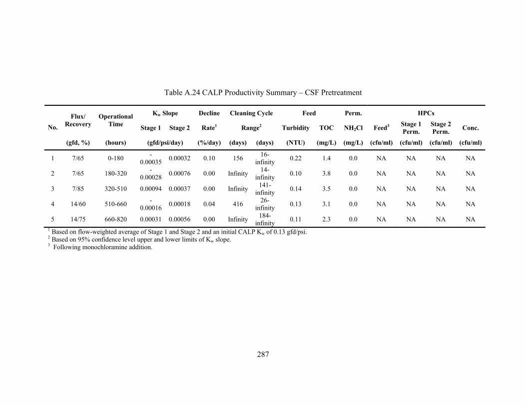
Table A.24 CALP Productivity Summary – CSF Pretreatment
Kw Slope Decline Cleaning Cycle Feed Perm. HPCs Flux/ Recovery
Operational Time Stage 1 Stage 2 Rate1 Range2 Turbidity TOC NH2Cl Feed3 Stage 1
Perm. Stage 2 Perm. Conc. No.
(gfd, %) (hours) (gfd/psi/day) (%/day) (days) (days) (NTU) (mg/L) (mg/L) (cfu/ml) (cfu/ml) (cfu/ml) (cfu/ml)
1 7/65 0-180 -0.00035 0.00032 0.10 156 16-
infinity 0.22 1.4 0.0 NA NA NA NA
2 7/65 180-320 -0.00028 0.00076 0.00 Infinity 14-
infinity 0.10 3.8 0.0 NA NA NA NA
3 7/85 320-510 0.00094 0.00037 0.00 Infinity 141-infinity 0.14 3.5 0.0 NA NA NA NA
4 14/60 510-660 -0.00016 0.00018 0.04 416 26-
infinity 0.13 3.1 0.0 NA NA NA NA
5 14/75 660-820 0.00031 0.00056 0.00 Infinity 184-infinity 0.11 2.3 0.0 NA NA NA NA
1 Based on flow-weighted average of Stage 1 and Stage 2 and an initial CALP Kw of 0.13 gfd/psi. 2 Based on 95% confidence level upper and lower limits of Kw slope. 3 Following monochloramine addition.
287
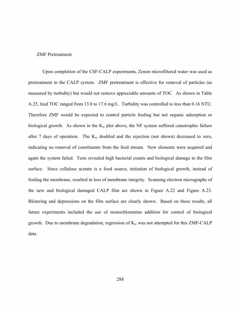
288
ZMF Pretreatment
Upon completion of the CSF-CALP experiments, Zenon microfiltered water was used as
pretreatment to the CALP system. ZMF pretreatment is effective for removal of particles (as
measured by turbidity) but would not remove appreciable amounts of TOC. As shown in Table
A.25, feed TOC ranged from 13.8 to 17.6 mg/L. Turbidity was controlled to less than 0.16 NTU.
Therefore ZMF would be expected to control particle fouling but not organic adsorption or
biological growth. As shown in the Kw plot above, the NF system suffered catastrophic failure
after 7 days of operation. The Kw doubled and the rejection (not shown) decreased to zero,
indicating no removal of constituents from the feed stream. New elements were acquired and
again the system failed. Tests revealed high bacterial counts and biological damage to the film
surface. Since cellulose acetate is a food source, initiation of biological growth, instead of
fouling the membrane, resulted in loss of membrane integrity. Scanning electron micrographs of
the new and biological damaged CALP film are shown in Figure A.22 and Figure A.23.
Blistering and depressions on the film surface are clearly shown. Based on these results, all
future experiments included the use of monochloramine addition for control of biological
growth. Due to membrane degradation, regression of Kw was not attempted for this ZMF-CALP
data.

289
Table A.25 CALP Productivity Summary – ZMF Pretreatment
Kw Slope Decline Cleaning Cycle Feed Perm. HPCs Flux/ Recovery
Operational Time Stage
1 Stage
2 Rate1 Range2 Turbidity TOC NH2Cl Feed3 Stage 1 Perm.
Stage 2 Perm. Conc. No.
(gfd, %) (hours) (gfd/psi/day) (%/day) (days) (days) (NTU) (mg/L) (mg/L) (cfu/ml) (cfu/ml) (cfu/ml) (cfu/ml)
1 7/65 820-985 na na na na na 0.15 13.8 0.0 na na na na
2 7/65 985-1125 na na na na na 0.16 17.6 0.0 na na na na 1 Based on flow-weighted average of Stage 1 and Stage 2 and an initial CALP Kw of 0.13 gfd/psi. 2 Based on 95% confidence level upper and lower limits of Kw slope. 3 Following monochloramine addition.
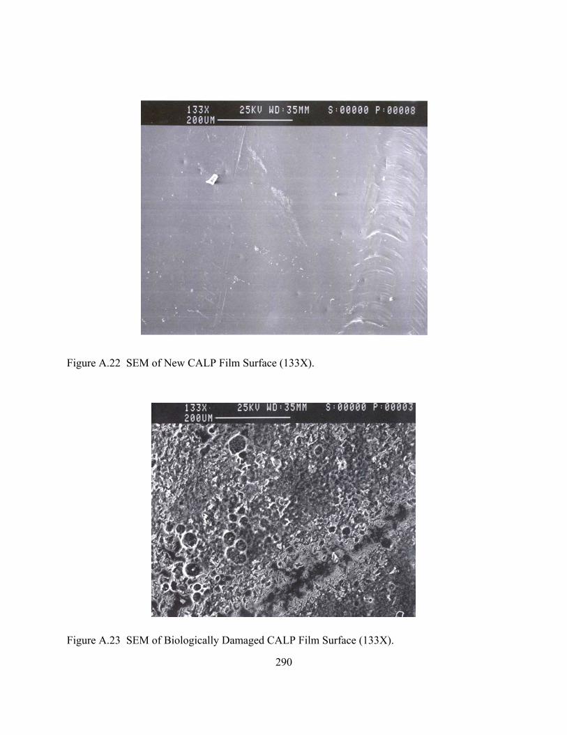
Figure A.22 SEM of New CALP Film Surface (133X).
Figure A.23 SEM of Biologically Damaged CALP Film Surface (133X).
290
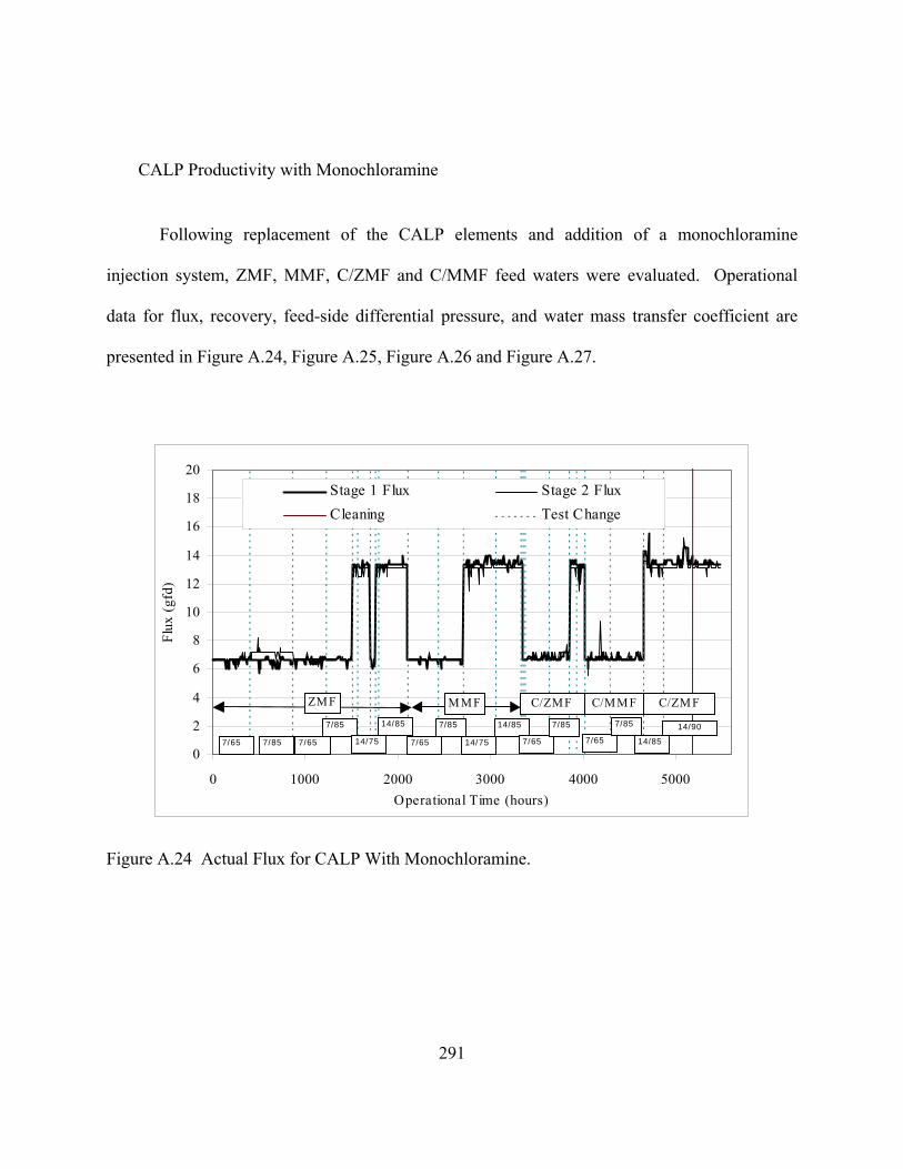
291
CALP Productivity with Monochloramine
Following replacement of the CALP elements and addition of a monochloramine
injection system, ZMF, MMF, C/ZMF and C/MMF feed waters were evaluated. Operational
data for flux, recovery, feed-side differential pressure, and water mass transfer coefficient are
presented in Figure A.24, Figure A.25, Figure A.26 and Figure A.27.
0
2
4
6
8
10
12
14
16
18
20
0 1000 2000 3000 4000 5000Operational Time (hours)
Flux
(gf
d)
Stage 1 Flux Stage 2 FluxCleaning Test Change
ZM F M M F C/M M F C/ZM FC/ZM F
7/65 7/85 7/65
7/85
14/75
14/85
7/65
7/85
14/75
14/85
7/65
7/85
7/65
7/85
14/85
14/90
Figure A.24 Actual Flux for CALP With Monochloramine.

0
10
20
30
40
50
60
70
80
90
100
0 1000 2000 3000 4000 5000Operational Time (hours)
Rec
over
y (%
)
Recovery Cleaning Tes t Change
ZM F M M F C/M M F C/ZM FC/ZMF
7/65 7/85 7/65
7/85
14/75
14/85
7/65
7/85
14/75
14/85
7/65
7/85
7/65
7/85
14/85
14/90
Figure A.25 Recovery for CALP With Monochloramine.
292
0
10
20
30
40
50
0 1000 2000 3000 4000 5000Operational Time (hours)
Feed
-sid
e P
ress
ure
Diff
eren
tial (
psi)
60
Stage 1 Stage 2 Cleaning Tes t Change
ZM F M M F C/M M F C/ZM FC/ZM F
7/65 7/85 7/65
7/85
14/75
14/85
7/65
7/85
14/75
14/85
7/65
7/85
7/65
7/85
14/85
14/90
Figure A.26 Actual Feed-Side Pressure Differential for CALP With Monochloramine.
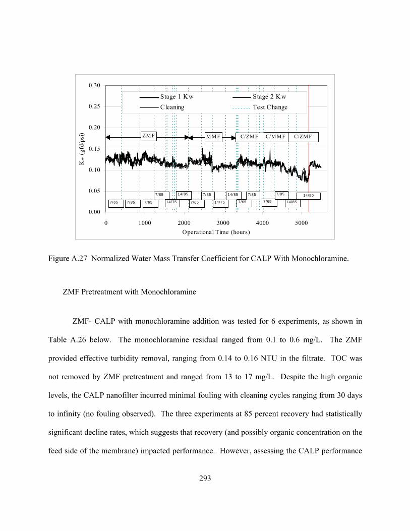
293
0.00
0 1000 2000 3000Operational Time (hour
0.05
0.10
0.15
0.20
0.25
0.30
4000 5000s)
Kw
(gf
d/ps
i)
Stage 1 Kw Stage 2 KwCleaning Test Change
ZM F M M F C/ZM FC/M M FC/ZM F
7/65 7/85 7/65
7/85
14/75
14/85
7/65
7/85
14/75
14/85
7/65
7/85
7/65
7/85
14/85
14/90
Coefficient for CALP With Monochloramine.
s tested for 6 experiments, as shown in
0.1 to 0.6 mg/L. The ZMF
0.14 to 0.16 NTU in the filtrate. TOC was
not rem g/L. Despite the high organic
levels, the C aning cycles ranging from 30 days
nts at 85 percent recovery had statistically
nic concentration on the
r, assessing the CALP performance
Figure A.27 Normalized Water Mass Transfer
ZMF Pretreatment with Monochloramine
ZMF- CALP with monochloramine addition wa
Table A.26 below. The monochloramine residual ranged from
provided effective turbidity removal, ranging from
oved by ZMF pretreatment and ranged from 13 to 17 m
ALP nanofilter incurred minimal fouling with cle
to infinity (no fouling observed). The three experime
significant decline rates, which suggests that recovery (and possibly orga
feed side of the membrane) impacted performance. Howeve

294
over the entire period of operation, it appears that the Kw was stable. Therefore, any decreases in
productivity appear to have been offset by slight increases in subsequent, lower recovery
experiments.
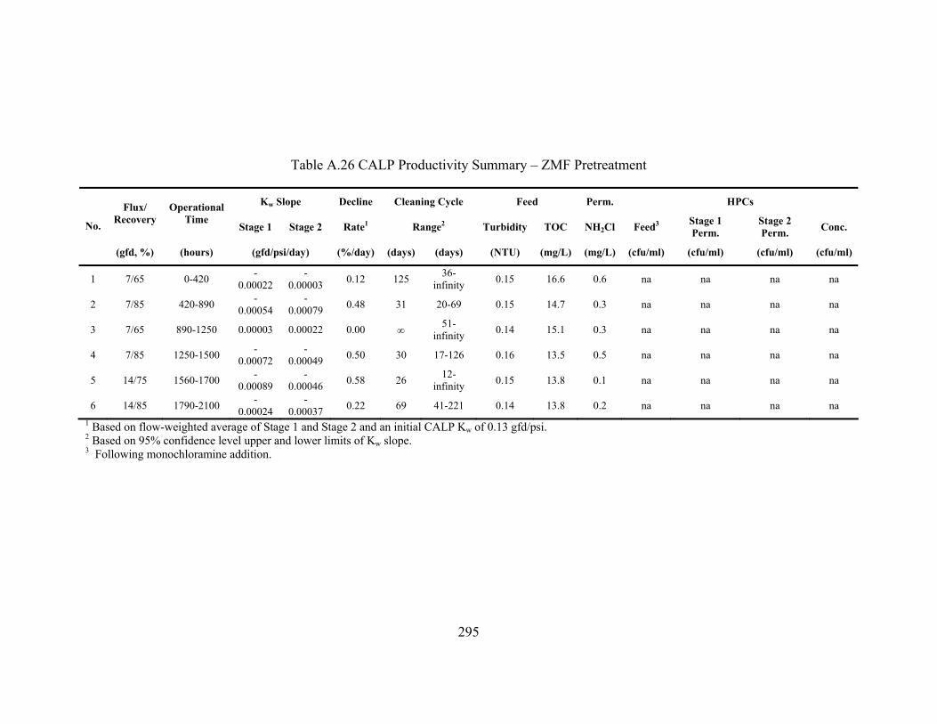
Table A.26 CALP Productivity Summary – ZMF Pretreatment
Kw Slope Decline Cleaning Cycle Feed Perm. HPCs Flux/ Recovery
Operational Time
Stage 1 Stage 2 Rate1 Range2 Turbidity TOC NH2Cl Feed3 Stage 1 Perm.
Stage 2 Perm. Conc. No.
(gfd, %) (hours) (gfd/psi/day) (%/day) (days) (days) (NTU) (mg/L) (mg/L) (cfu/ml) (cfu/ml) (cfu/ml) (cfu/ml)
1 7/65 0-420 -0.00022
-0.00003 0.12 125 36-
infinity 0.15 16.6 0.6 na na na na
2 7/85 420-890 -0.00054
-0.00079 0.48 31 20-69 0.15 14.7 0.3 na na na na
3 7/65 890-1250 0.00003 0.00022 0.00 ∞ 51-infinity 0.14 15.1 0.3 na na na na
4 7/85 1250-1500 -0.00072
-0.00049 0.50 30 17-126 0.16 13.5 0.5 na na na na
5 14/75 1560-1700 -0.00089
-0.00046 0.58 26 12-
infinity 0.15 13.8 0.1 na na na na
6 14/85 1790-2100 -0.00024
-0.00037 0.22 69 41-221 0.14 13.8 0.2 na na na na
1 Based on flow-weighted average of Stage 1 and Stage 2 and an initial CALP Kw of 0.13 gfd/psi. 2 Based on 95% confidence level upper and lower limits of Kw slope. 3 Following monochloramine addition.
295

296
MMF Pretreatment with Monochloramine
MMF pretreatment was tested with the CALP nanofilter for a total of four experiments.
Results are presented in Table A.27. Monochloramine residual in the permeate ranged from 0.7
to 1.0 mg/L. Heterotrophic plate counts were obtained for the first and last experiments.
Turbidity was effectively controlled by MMF pretreatment and ranged from 0.13 to 0.15 NTU.
TOC concentrations in the NF feed ranged from 4.1 to 12.1 mg/L. As shown, the first
experiment at 7 gfd flux and 65% recovery incurred a statistically significant decline in Kw that
resulted in an estimated cleaning cycle of 54 days. This system had the highest feed TOC
concentration, 12.1 mg/L, of the four experiments. The HPC counts in the concentrate (180,000
cfu/ml) were 2 log orders higher than expected, based on a feed concentration of 2,000 cfu/ml
and a concentration factor of 2.2. Therefore the monochloramine addition may not have been
effective for biological control and the system may have suffered from slight fouling. Damage to
the membrane did not appear to occur but sustained operation with high levels of HPCs in the
permeate could have resulted in membrane failure. This experiment can be compared to the last
experiment, at 14 gfd flux and 85% recovery, which did not incur statistically significant fouling
even at these higher settings. However, feed TOC was only 4.1 mg/L and HPCs were low in all
samples. In summary, MMF-CALP productivity appeared steady at all settings with the
exception of slight fouling at low flux and recovery that may have been due to biological growth.
Given the susceptibility of cellulose acetate membranes to biological degradation, this is of
concern and warrants consideration of higher monochloramine concentrations in future research.

Table A.27 CALP Productivity Summary – MMF Pretreatment
Kw Slope Decline Cleaning Cycle Feed Perm. HPCs Flux/ Recovery
Operational Time
Stage 1 Stage 2 Rate1 Range2 Turbidity TOC NH2Cl Feed3 Stage 1 Perm.
Stage 2 Perm. Conc. No.
(gfd, %) (hours) (gfd/psi/day) (%/day) (days) (days) (NTU) (mg/L) (mg/L) (cfu/ml) (cfu/ml) (cfu/ml) (cfu/ml)
1 7/65 2100-2430 -0.00039
-0.00032 0.28 54 30-228 0.14 12.1 0.7 2,000 1,000 1,000 180,000
2 7/85 2430-2710 0.00029 -0.00057 0.00 ∞ 27-
infinity 0.15 8.6 1.0 na na na na
3 14/75 2710-3050 0.00069 0.00037 0.00 ∞ Infinity 0.13 5.7 1.0 na na na na
4 14/85 3050-3325 -0.00018
-0.00012 0.12 123 40-
infinity 0.14 4.1 0.8 12,600 39 8 9,650 1 Based on flow-weighted average of Stage 1 and Stage 2 and an initial CALP Kw of 0.13 gfd/psi. 2 Based on 95% confidence level upper and lower limits of Kw slope. 3 Following monochloramine addition.
297

298
C/ZMF Pretreatment with Monochloramine
C/ZMF pretreatment was evaluated during two periods of operation for a total of seven
experiments, as shown in Table A.28. C/ZMF was effective for both particle and TOC removal.
Feed turbidity ranged from 0.10 to 0.15 NTU and TOC from 3.0 to 5.3 mg/L. Permeate
monochloramine concentration ranged from 0.7 to 1.8 mg/L. Estimated cleaning cycles ranged
from 22 days to infinity (no fouling observed). Three of the seven experiments showed fouling.
However, due to data variability, the upper and lower 95% confidence limits indicated a broad
range of possible cleaning cycles for most experiments. For example, none of the slopes for the
seven experiments were statistically different from zero (which would indicate no fouling).
Conversely, the lower limit of the 95% confidence level indicated cleaning cycles could be as
short as 6 days or less, for four of the seven experiments. This suggests that limited
interpretation of the individual experiments is possible.
HPC values suggested possible biogrowth in the sixth experiment, with a concentrate
level of 2,510 cfu/ml compared to 2 cfu/ml in the feed. However, feed levels of 1,000 – 5,000
cfu/ml were common in other experiments using the CALP membrane and monochloramine
therefore the concentrate value of 2,510 cfu/ml may not be indicative of attached bacterial
growth on the membrane film.

Table A.28 CALP Productivity Summary – C/ZMF Pretreatment
Kw Slope Decline Cleaning Cycle Feed Perm. HPCs Flux/ Recovery
Operational Time
Stage 1 Stage 2 Rate1 Range2 Turbidity TOC NH2Cl Feed3 Stage 1 Perm.
Stage 2 Perm. Conc. No.
(gfd, %) (hours) (gfd/psi/day) (%/day) (days) (days) (NTU) (mg/L) (mg/L) (cfu/ml) (cfu/ml) (cfu/ml) (cfu/ml)
1 7/65 3375-3635 -0.00036
-0.00028 0.25 59 21-
infinity 0.11 3.1 1.2 4,500 11 122 170
2 7/85 3635-3855 -0.00047 0.00040 0.14 107 26-
infinity 0.14 3.0 1.2 na na na na
3 14/75 3855-3925 -0.00050
-0.00160 0.67 22 5-infinity 0.13 3.1 0.7 na na na na
4 14/85 3925-4025 0.00142 0.00200 0.00 ∞ 53-infinity 0.15 3.5 0.7 5 201 125 285
5 14/85 4650-4870 0.00362 0.00528 0.00 infinite 6-infinity 0.10 5.1 1.8 na na na na
6 14/90 4870-5185 0.00154 0.00216 0.00 infinite 3-infinity 0.13 5.0 1.1 2 32 33 2,510
7 14/90 5185-5485 0.00231 0.00163 0.00 infinite 5-infinity 0.11 5.3 1.3 na na na na 1 Based on flow-weighted average of Stage 1 and Stage 2 and an initial CALP Kw of 0.13 gfd/psi. 2 Based on 95% confidence level upper and lower limits of Kw slope. 3 Following monochloramine addition.
299

300
C/MMF Pretreatment
C/MMF pretreatment was evaluated during two experiments, as shown in Table A.29, at
7 gfd flux and 65 and 85 percent recovery. C/MMF reduced turbidity to less than 0.14 NTU.
However, low coagulant doses resulted in minimal reduction in TOC values. Feed TOC ranged
from 15.3 to 18.3 mg/L. Permeate monochloramine concentration ranged from 0.8 to 1.2 mg/L.
Estimated cleaning cycles ranged from 13 to 56 days with the shorter run time associated with
the higher recovery experiment. The first experiment, at 7 gfd flux and 65 percent recovery,
suffered from biological growth as shown by HPC counts in the permeate and concentrate well
above the feed level. Additionally, results were variable for this experiment and the 95%
confidence level cleaning cycle ranged from 19 days to infinity, limiting the interpretation of this
experiment. The second experiment, at 7 gfd flux and 85 percent recovery, resulted in more
stable data and a more reliable range of cleaning cycles of 11 to 17 days. Therefore it appears
that the higher recovery may have resulted a shorter run time. The impact of biological growth
on fouling rate could not be determined since HPC measurements were not obtained for the
second experiment.

301
Table A.29 CALP Productivity Summary – C/MMF Pretreatment
Kw Slope Decline Cleaning Cycle Feed Perm. HPCs Flux/ Recovery
Operational Time
Stage 1 Stage 2 Rate1 Range2 Turbidity TOC NH2Cl Feed3 Stage 1 Perm.
Stage 2 Perm. Conc. No.
(gfd, %) (hours) (gfd/psi/day) (%/day) (days) (days) (NTU) (mg/L) (mg/L) (cfu/ml) (cfu/ml) (cfu/ml) (cfu/ml)
1 7/65 4025-4295 -0.00016
-0.00073 0.27 56 19-infinity 0.14 15.3 0.8 805 2,085 388 25,400
2 7/85 4295-4650 -0.00143
-0.00160 1.14 13 11-17 0.12 18.3 1.2 na na na na
1 Based on flow-weighted average of Stage 1 and Stage 2 and an initial CALP Kw of 0.13 gfd/psi. 2 Based on 95% confidence level upper and lower limits of Kw slope. 3 Following monochloramine addition.
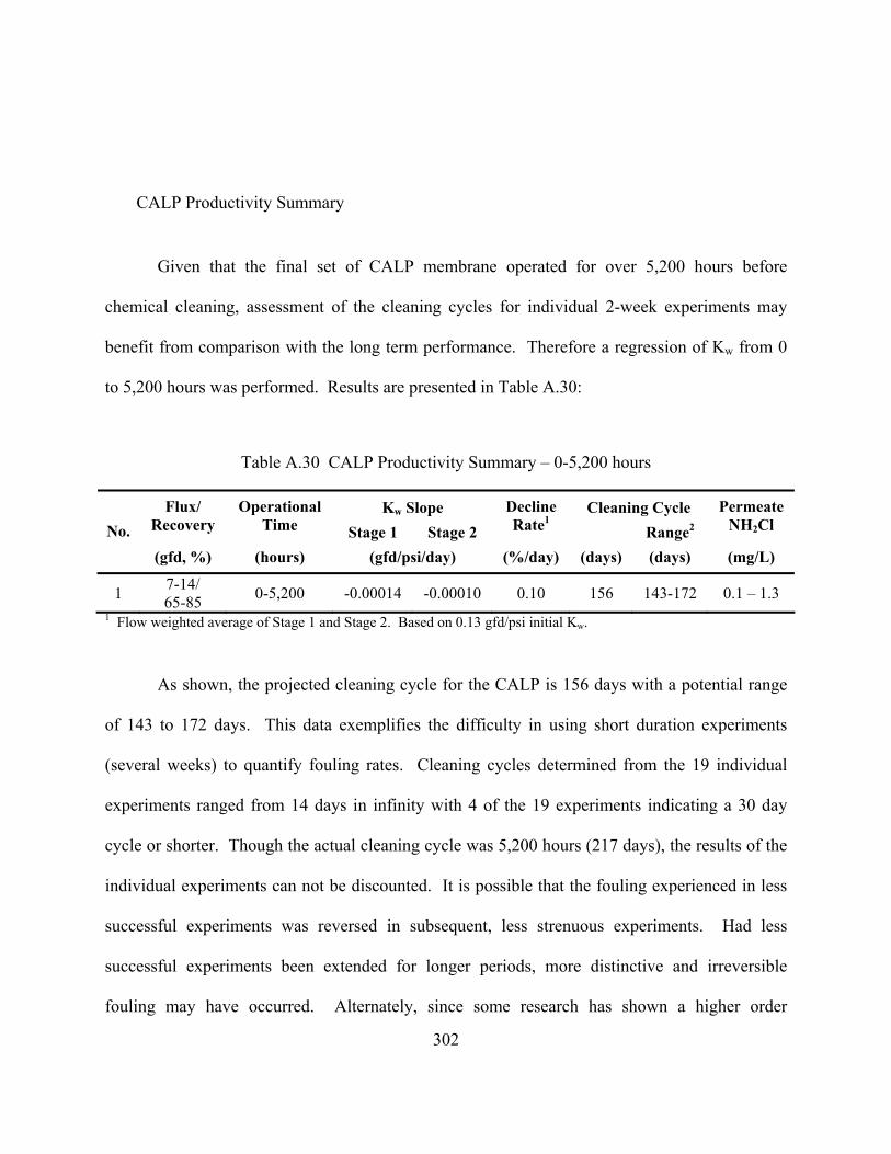
302
CALP Productivity Summary
Given that the final set of CALP membrane operated for over 5,200 hours before
chemical cleaning, assessment of the cleaning cycles for individual 2-week experiments may
benefit from comparison with the long term performance. Therefore a regression of Kw from 0
to 5,200 hours was performed. Results are presented in Table A.30:
Table A.30 CALP Productivity Summary – 0-5,200 hours
Kw Slope Cleaning Cycle Flux/ Recovery
Operational Time Stage 1 Stage 2
Decline Rate1
Range2
Permeate NH2Cl No.
(gfd, %) (hours) (gfd/psi/day) (%/day) (days) (days) (mg/L)
1 7-14/ 65-85 0-5,200 -0.00014 -0.00010 0.10 156 143-172 0.1 – 1.3
1 Flow weighted average of Stage 1 and Stage 2. Based on 0.13 gfd/psi initial Kw.
As shown, the projected cleaning cycle for the CALP is 156 days with a potential range
of 143 to 172 days. This data exemplifies the difficulty in using short duration experiments
(several weeks) to quantify fouling rates. Cleaning cycles determined from the 19 individual
experiments ranged from 14 days in infinity with 4 of the 19 experiments indicating a 30 day
cycle or shorter. Though the actual cleaning cycle was 5,200 hours (217 days), the results of the
individual experiments can not be discounted. It is possible that the fouling experienced in less
successful experiments was reversed in subsequent, less strenuous experiments. Had less
successful experiments been extended for longer periods, more distinctive and irreversible
fouling may have occurred. Alternately, since some research has shown a higher order
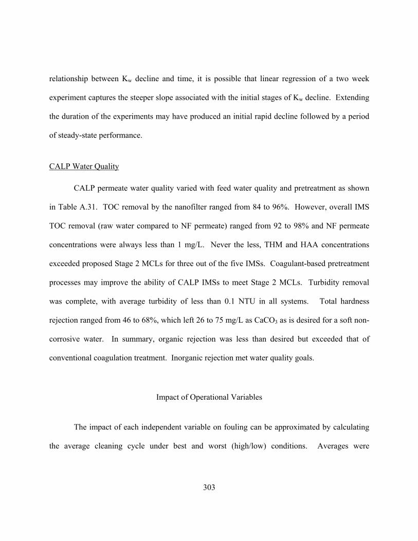
relationsh
303
ip between Kw decline and time, it is possible that linear regression of a two week
experiment captures the steeper slope associated with the initial stages of Kw decline. Extending
the duration of the experiments may have produced an initial rapid decline followed by a period
of steady-state performance.
CALP Water Quality
CALP permeate water quality varied with feed water quality and pretreatment as shown
in Table A.31. TOC removal by the nanofilter ranged from 84 to 96%. However, overall IMS
TOC removal (raw water compared to NF permeate) ranged from 92 to 98% and NF permeate
concentrations were always less than 1 mg/L. Never the less, THM and HAA concentrations
exceeded proposed Stage 2 MCLs for three out of the five IMSs. Coagulant-based pretreatment
processes may improve the ability of CALP IMSs to meet Stage 2 MCLs. Turbidity removal
was complete, with average turbidity of less than 0.1 NTU in all systems. Total hardness
rejection ranged from 46 to 68%, which left 26 to 75 mg/L as CaCO3 as is desired for a soft non-
corrosive water. In summary, organic rejection was less than desired but exceeded that of
conventional coagulation treatment. Inorganic rejection met water quality goals.
Impact of Operational Variables
The impact of each independent variable on fouling can be approximated by calculating
the average cleaning cycle under best and worst (high/low) conditions. Averages were

calculated from
the resu
•
improving perform
limited and the la
was unexpected and suggests that flux m
independent variables. However, statistic
304
the cleaning cycles determined using the linear model, presented previously in
lts section. Results are presented in Table A.32. As shown, fouling was minimized with:
Use of coagulant-based pretreatment processes (CSF, C/ZMF, and C/MMF);
• Lower recovery;
• Use of monochloramine; and
• Lower TOC.
The impacts of flux and turbidity were inconsistent by membrane, with lower values
ance in some cases and but not others. The range of turbidity observed was
ck of consistency was expected. The lack of consistency in the impact of flux
ay not be as critical a factor in fouling that the other
al regression may provide more insight.

F Perm.
0.7 65 47
0.08
305
Table A.31 CALP Water Quality Summary
CSF ZMF MMF C/ZMF C/MM
Analyte Units Raw Feed Perm. Raw Feed Perm. Raw Feed Perm. Raw Feed Perm. Raw Feed
TOC mg/L 20.7 3.2 0.5 17.4 15.0 0.8 6.2 5.5 0.5 15.5 4.2 0.8 19.2 16.3 SDS-THM µg/L 1556 124 57 1352 1037 60 469 443 34 1032 152 35 1545 1244
SDS-HAA(6) µg/L 1628 51 19 2313 1868 57 591 362 23 1467 683 21 4073 1756 Turbidity NTU 2.55 0.14 0.08 2.39 0.16 0.09 1.61 0.15 0.09 2.0 0.14 0.09 1.72 0.13
TH mg/L as CaCO3 114 181 61 81 78 26 168 163 75 116 116 50 103 101 51 Chloride mg/L 13 16 14 10 36 25 16 64 45 13 46 38 13 96 64 Sulfate mg/L 15 109 14 10 11 1 35 34 4 18 111 14 10 10 <1

306
Table A.32 Estimated Effects of Operating Conditions and Feed Water Quality on Nanof leaning Cycle.
Cleaning Cycle (days)
ilter C
Coagulant-based Pretreatment?
Flux (gfd)
Recovery (%) Biocide? Feed Turbidity
(NTU) Feed TOC
(mg/L) NF
Yes No 7 14 65 85 Yes No < median > median < median > medianCALP 80 65 59 101 103 57 NA NA 81 59 135 50 ESNA 25 6 25 25 28 22 NA NA 25 6 26 9 LFC1 30 6 13 7 16 7 12 7 7 10 13 6
Experiments that combined the favorable conditions for each factor (coagulant addition, biocide addition, and low flux, recovery, turbidity, and TOC) experienced no fouling.

MODELING OF PILOT RESULTS
Based on the resistance models presented previously, model M2 is appropriate for this
pilot data, in which both flux and pressure varied. Model M2 was used for regression and
evaluation of pilot results:
KR
r C VA
r C VA
r C Y VA
w
mpart S ads O bio A obs
=+ + +
⎛⎝⎜
⎞⎠⎟
1
µ
(A.35)
Turbidity was used as a measure of Cs,, the particle loading. For CO, the measure of
organic concentration, two parameters were measured, TOC and UV-254. UV-254 is reported to
measure the aromatic fraction of organic matter, which is reportedly more likely to cause organic
adsorptive fouling. Therefore, these two parameters were compared for modeling of organic
adsorptive fouling. For CAYobs, the measure of biological growth, parameters such as
assimilable organic carbon (AOC) organic carbon (BDOC) were
desired but were not obtainable monochloramine concentration is
available and would have an inverse relationship with biological growth. Additionally,
heterotrophic plate counts are av on of the data. HPCs can be a measure of the
attached bacteria growth since releas attached colonies is expected to occur and
would increase HPC levels in the concentrate.
A summary of data from own in Table A.33 below. As shown,
turbidity data is available for approximately one out of every four Kw data points. TOC and UV-
or biologically degradable
during pilot testing. However,
ailable for a porti
e of bacteria from
the pilot testing is sh
307

308
254 data were only collected once every two weeks compared to Kw data that was collected three
times per day. TOC and UV-254 were linearly extrapolated with time, for the periods between
sampling events. This was acceptable given the relatively slow changes in feed water TOC and
UV-254 with time. Though abrupt changes occasionally occur due to significant rain events,
Figure A.28 shows the pilot raw water TOC data compared to raw water TOC obtained by the
water treatment plant. Changes in raw water TOC were linear within the two-week periods
between pilot water quality sampling events.
For monochloramine addition, as shown in Table A.33, significant data are available for
the LFC1 and CALP. However, monochloramine was not used for the ESNA and was always
used for the CALP, following the biological degradation of the first set of CALP elements.
Therefore regressions designed to determine the effect of monochloramine addition are only
applicable to the LFC1. HPC data were not collected for the ESNA and were only collected six
times for the CALP. Given that monochloramine addition was continuous for the CALP and loss
of integrity would have occurred if biological growth were present, as happened with the first set
of CALP membranes, biological fouling was not considered a factor for the CALP. HPC data
for the LFC1 were collected 22 times and should be sufficient for modeling.

309
Table A.33 Pilot Data Summary
Turbidity TOC UV-254 Monochloramine HPC NF No. Kw Obs. No. Obs. (NTU) No. Obs. (mg/L) No. Obs. (cm-1) No. Obs. (mg/L) No. Obs. (cfu/ml) ESNA 213 45 0.11 5 3.0 5 0.0383 NA NA1 NA NA LFC1 672 152 0.15 17 15.6 17 0.6947 160 1.0 22 CALP 828 172 0.14 24 9.7 24 0.3850 195 1.5 6 1 – monochloramine not used with ESNA.
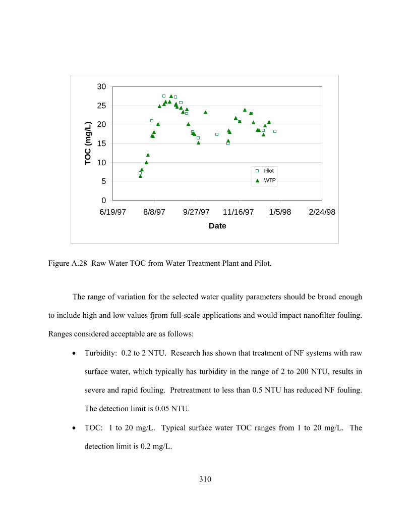
0
5
10
15
20
25
30
6/19/97 8/8/97 9/27/97 11/16/97 1/5/98 2/24/98
Date
TOC
(mg/
L)
Pilot
WTP
Figure A.28 Raw Water TOC from Water Treatment Plant and Pilot.
The range of variation for the selected water quality parameters should be broad enough
to include high and low values fjrom full-scale applications and would impact nanofilter fouling.
Ranges considered acceptable are as follows:
• Turbidity: 0.2 to 2 NTU. Research has shown that treatment of NF systems with raw
surface water, which typically has turbidity in the range of 2 to 200 NTU, results in
severe and rapid fouling. Pretreatment to less than 0.5 NTU has reduced NF fouling.
The detection limit is 0.05 NTU.
• TOC: 1 to 20 mg/L. Typical surface water TOC ranges from 1 to 20 mg/L. The
detection limit is 0.2 mg/L.
310
311
• UV-254: 0.1 to 1.0 cm-1. Typical surface water UV-254 ranges from 0.1 to 1.0 cm-1.
The detection limit is 0.0001 cm-1.
• Monochloramine: 0 to 4 mg/L. Absence of a monochloramine residual would allow
for biological growth while 4 mg/L represents the Maximum Residual Disinfectant
Level acceptable in drinking water. The detection limit is 0.1 mg/L.
• Heterotrophic Plate Counts: 0 to 103 cfu/mL. Absence of positive HPC
measurements would indicate full control of biogrowth whereas large populations, on
the order of 103-105 cfu/mL, have been observed in NF systems suffering from
biological growth.
A histogram for raw water TOC, feed turbidity. feed TOC, feed UV254, stage 1 HPCs,
stage 2 HPCs and NH2Cl dose is presented in Figure A.29, Figure A.30, Figure A.31, Figure
A.32, Figure A.33 and Figure A.34 respectively.

Turbidity (NTU)
.30.28.25.23.20.17.15.13.10.08
No. o
f Obs
erva
tions
600
500
400
300
200
100
0
Std. Dev = .04 Mean = .14
N = 1713.00
Figure A.29 Nanofilter Feed Turbidity.
TOC (mg/L)
191715131197531
No. o
f Obs
erva
tions
300
200
100
0
Std. Dev = 6.23 Mean = 9
N = 1713.00
Figure A.30 Nanofilter Feed TOC.
312

UV-254 (1/cm)
1.00.90.80.70.60.50.40.30.20.100.00
No. o
f Obs
erva
tions
300
200
100
0
Std. Dev = .32 Mean = .38
N = 1713.00
400
Figure A.31 Nanofilter Feed UV-254.
313
Average Feed-Side HPC Concentration (cfu/ml)
100,00080,00060,00040,00020,0000
No.
of O
bser
vatio
ns
300
200
100
0
Std. Dev = 27342.68 Mean = 21473
N = 524.00
Figure A.32 Nanofilter Average Stage 1 HPC.

Average Feed-Side HPC Concentration
120000100000800006000040000200000
No.
of O
bser
vatio
ns 200
100
0
Std. Dev = 26656.00 Mean = 18991
N = 524.00
300
Figure A.33 Nanofilter Average Stage 2 HPC.
314
Monochloramine (mg/L)
9.08.07.06.05.04.03.02.01.00.0
No. o
f Obs
erva
tions
700
600
500
400
300
200
100
0
Std. Dev = 1.61 Mean = 1.4
N = 1713.00
Figure A.34 Nanofilter Monochloramine Dose.
315
Pretreatment systems reduced feed water turbidity to less than 0.3 NTU in all cases. At
this low level, particle fouling is expected to have been fully controlled in the pilot tests
conducted for this research. Previous research by Taylor et al.. (1992) has shown that
operational times can be extended from 2 days to as much as 20 days when feed turbidity is
reduced from 2 NTU to less than 0.5 NTU, as shown in Figure A.35. This previous research
attributed the remaining productivity decline to organic adsorption and/or biofouling but
eliminated particle plugging below 0.5 NTU turbidity. Research by Elemelich et al.. (1997)
utilized 90 mg/L of silica colloids to produce particle fouling in bench applications. Finally,
industry standards, including manufacturer warranty specifications, require that nanofilter feed
turbidity be less than 1 NTU, indicating that the levels of turbidity feed to the pilot units in this
study (< 0.3 NTU) would be sufficiently low that particle fouling would not be expected to
occur.
Therefore it is believed that the range in turbidity observed in these field tests may not be
adequate for reliable assessment of particle fouling. However, the effective removal of tubidity
by the pretreatment processes is a desired outcome that supports use of these pretreatment
processes in Integrated Membrane Systems and precludes the need for quantification of the
effect of varying turbidity on NF fouling. The ranges observed for the remaining parameters are
considered sufficiently broad to quantify fouling effects.

316
ACSF-EACSF-F
BAC-E
MF-E
BAC-F
0.0
0.5
1.0
1.5
2.0
0 5 10 15 20 25
Cleaning Cycle (days)
Turb
idity
(NTU
)
BAC-F: biologically active carbon filtration – nanofiltration membrane F BAC-E: biologically active carbon filtration – nanofiltration membrane E MF-E: microfiltration – nanofiltration membrane E ACSF-E: alum coagulation, sedimentation, filtration – nanofiltration membrane E ACSF-F: alum coagulation, sedimentation, filtration – nanofiltration membrane F
Figure A.35 Effect of Feed Water Turbidity on Cleaning Cycle (Taylor 1992).
Based on these assessments, data for each NF membrane were first regressed to fit the
linear and resistance models, based on operational time. Results are summarized in Table A.34.
As shown, the linear model with time produced a higher coefficient of determination in all cases
except were time was not statistically significant. The sign of the coefficient for the linear model
was negative in all cases, as expected, indicating Kw decreased with time. The sign of the
coefficient for the resistance model was positive for all cases except Stage 2 LFC1, again
indicating that Kw decreased with time. The LFC1 Kw increased with time as described
previously, due to film degradation. It is expected that regression based on time for the LFC1
will produce limited results, due to the degradation and loosening of the membrane film, as is
shown by two of the four LFC1 permutations being statistically insignificant in Table A.34.

Given that m
oxidation, as occurred with the LF
be as applic
summary, these resu
this data. Tim
317
embrane water treatment facilities are not designed for film damage due to
C1 during monochloramine addition, modeling results will not
able to the engineering community as will results for the ESNA and CALP. In
lts indicate that, with respect to time, the linear model is more applicable to
e is not an adequate factor for modeling of the LFC1 performance.
Table A.34 Modeling Results for Operational Time
Linear Model KβK W1w O
tβ 2+=
Resistance Model
tR1K
2M1w β+β
= NF Stage
R2 R2 β2
1 0.91 0.84 6.94E-02 β2
-0.00218 ESNA 2 0.76 0.75 1.78E-02 1 0.75 -0.00045 0.73 NS LFC1 2 0.57 NS 0.57 -3.57E-03 1 0.50 -0.00016 0.47 1.18E-02 CALP 2 0.44 -0.00011 0.43 8.86E-03
Though the range for the turbidity data is na wer than desired, the original multivariate
model for particle, organic, and biological fouling was regressed as shown in Table A.35. Again
the linear regression was found to fit the data better, in terms of the coefficient of determination.
Turbidity was not statistically significant in most cases, as expected. Additionally, the sign on
the turbidity coefficient indicated increased fouling with decrease turbidity, which is contrary to
logic and past research. Thus turbidity was not evaluated further in this regression effort. Total
organic carbon concentration was statistically significant and indicated increasing fouling with
increasing mass of TOC, in all cases. Therefore organic adsorption and/or substrate-limited
-0.00057
rro

318
biological growth appear to be significant for all systems. Monochloramine mass was significant
in all cases where data were available (CALP and LFC1). For the LFC1, Kw increased with
increasing monochloramine mass. This result supports the film degradation discussed previously
and indicates the LFC1 is not monochloramine tolerant. For the CALP, Kw decreased with
increasing monochloramine mass.
The significance of TOC versus UV-254 as an organic parameter was assessed since
TOC has historical precedence but UV-254 is a quicker and less expensive analysis.
Additionally, UV-254 measures the aromatic fraction of organic carbon. Only the linear model
was evaluated, with monochloramine mass, as shown in Table A.36. Organic concentrations
were shown to be significant and cause a decline in Kw, for both TOC and UV-254. Comparison
between NF membranes and stages shows the same ranking, based on the coefficients for UV-
254 or for TOC. Therefore UV-254 appears to follow TOC such that similar conclusions can be
drawn using either parameter.

319
Table A.35 Modeling Results for Particle, Organic, and Biological Fouling
Linear Model Cl4TOC3P2W1w MMMKK
Oβ+β+β+β=
Resistance Model
Cl4TOC3P2M1w MM
1MR
1Kβ+β+β+β
=
NF Stage
R2 β2 β3 β4 R2 β2 β3 β4
1 0.94 NS -1.11E-04 NA 0.92 -0.154 7.05E-03 NA ESNA 2 0.77 NS -2.83E-05 NA 0.77 NS 9.88E-04 NA 1 0.92 NS -4.87E-05 5.41E-04 0.79 NS 2.09E-03 -2.18E-02 LFC1 2 0.75 7.79E-04 -2.30E-05 1.56E-04 0.72 -3.93E-02 1.10E-03 -6.78E-03 1 0.67 5.15E-03 -1.39E-05 -6.51E-04 0.61 -3.94E-01 9.94E-04 5.16E-02 CALP 2 0.56 2.90E-03 -9.45E-06 -4.28E-04 0.53 -0.228 7.17E-04 3.44E-02
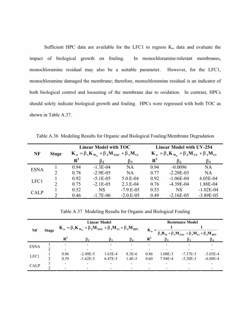
Sufficient HPC data are available for the LFC1 to regress Kw data and evaluate the
impact of biological growth on fouling. In monochloramine-tolerant membranes,
monochloramine residual may also be a suitable parameter. However, for the LFC1,
monochloramine damaged the membrane; therefore, monochloramine residual is an indicator of
both biological control and loosening of the membrane due to oxidation. In contrast, HPCs
should solely indicate biological growth and fouling. HPCs were regressed with both TOC as
shown in Table A.37.
Table A.36 Modeling Results for Organic and Biological Fouling/Membrane Degradation
Linear Model with TOC Linear Model with UV-254 Cl3TOC2W1w MMKK
Oβ+β+β= Cl3UV2W1w MMKK
Oβ+β+β= NF Stage
R2 β2 β3 R β2 β3
1 0.94 -1.3E-04 NA 0.94 -0.0096 NA
2
ESNA 2 0.78 -2.9E-05 NA 0.77 -2.20E-03 NA 1 0.92 -5.1E-05 5.0.E-04 0.92 -1.06E-04 4.05E-04 LFC1 2 0.75 -2.1E-05 2.3.E-04 0.76 -4.39E-04 1.88E-04 1 0.52 NS -7.9.E-05 0.53 NS -1.02E-04 CALP 2 0.46 -1.7E-06 -2.0.E-05 0.49 -2.16E-05 -3.89E-05
Table A.37 Modeling Results for Organic and Biological Fouling
Linear Model HPC4Cl3TOC2W1w MMMKK
Oβ+β+β+β=
Resistance Model
HPC4Cl3TOC2M1w MM
1MR
1K
β+β+β+β= NF Stage
R2 β2 β3 β4 R β2 β3 β4
1 - - - - - - - -
2
ESNA 2 - - - - - - - - 1 0.86 -2.49E-5 1.63E-4 8.3E-6 0.86 1.08E-3 -7.37E-3 -3.03E-4 LFC1 2 0.59 -1.62E-5 6.47E-5 1.4E-5 0.60 7.94E-4 -3.20E-3 -6.88E-4 1 - - - - - - - - CALP 2 - - - - - - - -
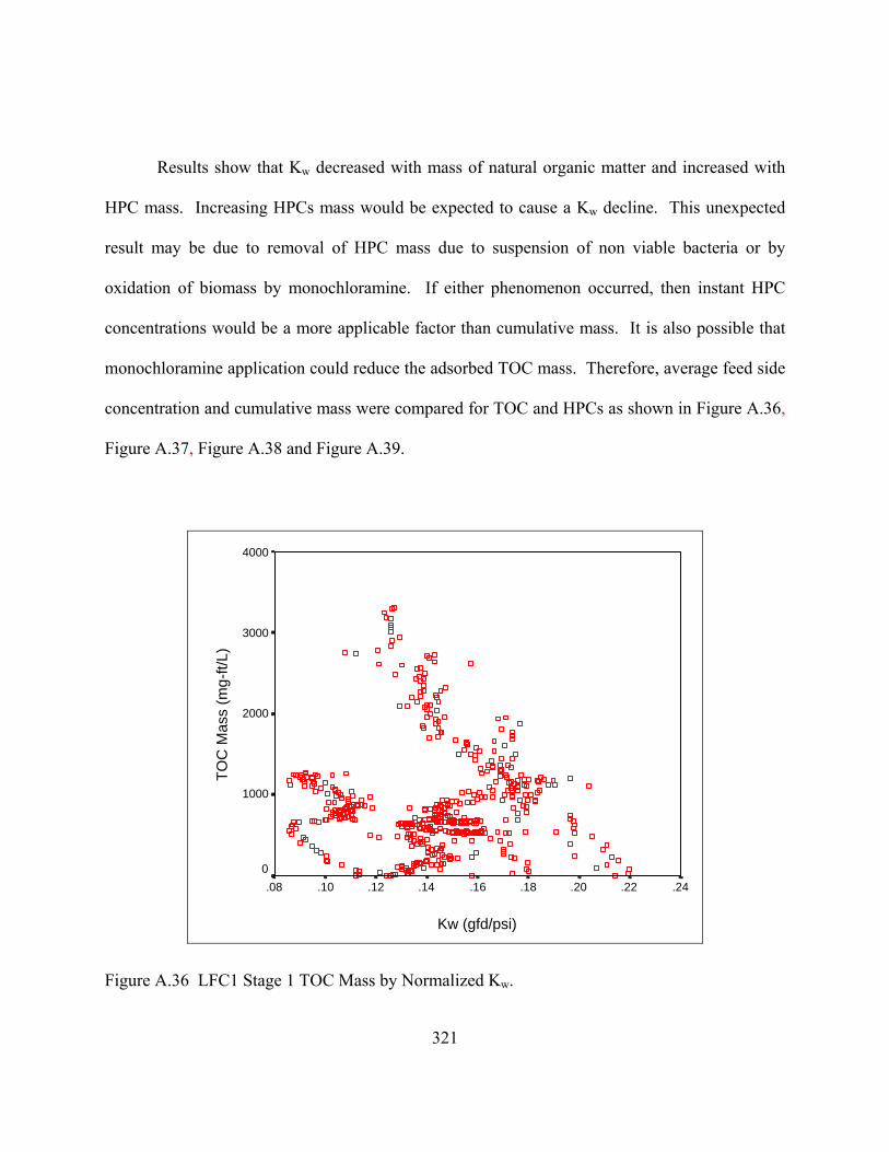
321
Results show that Kw decreased with mass of natural organic matter and increased with
HPC mass. Increasing HPCs mass would be expected to cause a Kw decline. This unexpected
result may be due to removal of HPC mass due to suspension of non viable bacteria or by
oxidation of biomass by monochloramine. If either phenomenon occurred, then instant HPC
concentrations would be a more applicable factor than cumulative mass. It is also possible that
monochloramine application could reduce the adsorbed TOC mass. Therefore, average feed side
concentration and cumulative mass were compared for TOC and HPCs as shown in Figure A.36,
Figure A.37, Figure A.38 and Figure A.39.
Kw (gfd/psi)
.24.22.20.18.16.14.12.10.08
TOC
Mas
s (m
g-ft/
L)
4000
3000
2000
1000
0
Figure A.36 LFC1 Stage 1 TOC Mass by Normalized Kw.
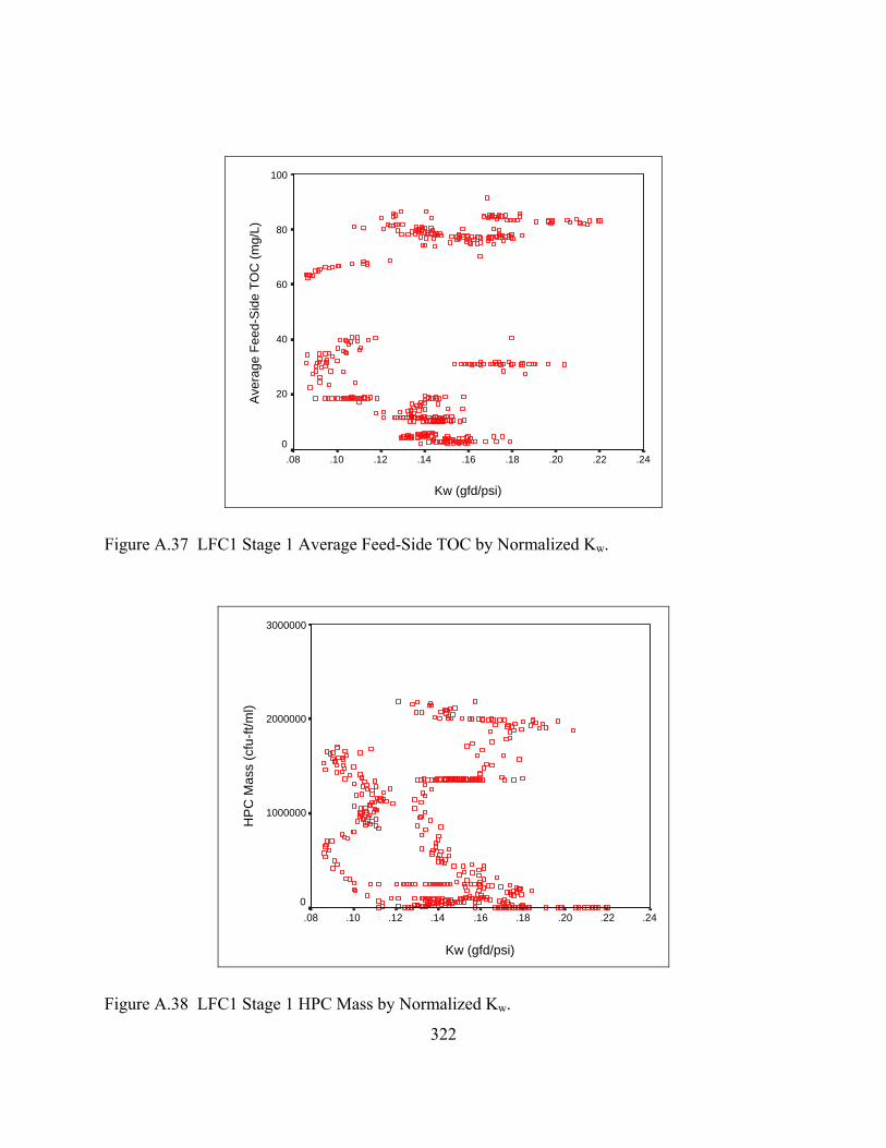
Kw (gfd/psi)
.24.22.20.18.16.14.12.10.08
Ave
rage
Fee
d-S
ide
TOC
(mg/
L)
100
80
60
40
20
0
Figure A.37 LFC1 Stage 1 Average Feed-Side TOC by Normalized Kw.
Kw (gfd/psi)
.24.22.20.18.16.14.12.10.08
HP
C M
ass
(cfu
-ft/m
l)
3000000
2000000
1000000
0
Figure A.38 LFC1 Stage 1 HPC Mass by Normalized Kw.
322
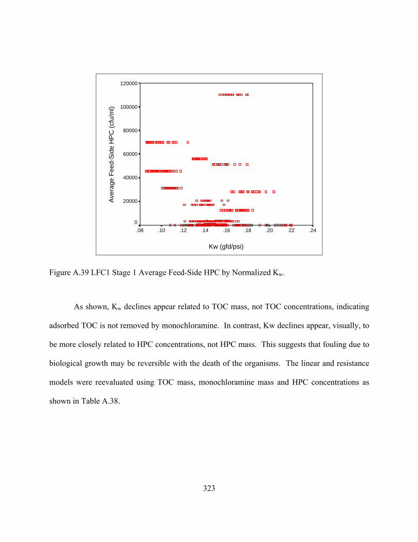
Kw (gfd/psi)
.24.22.20.18.16.14.12.10.08
Ave
rage
Fee
d-S
ide
HP
C (c
fu/m
l) 100000
80000
60000
40000
20000
0
120000
As shown, Kw declines appear related to TOC mass, not TOC concentrations, indicating
adsorbed TOC is not removed by monochloramine. In contrast, Kw declines appear, visually, to
be more closely related to HPC concentrations, not HPC mass. This suggests that fouling due to
biological growth may be reversible with the death of the organisms. The linear and resistance
models were reevaluated using TOC mass, monochloramine mass and HPC concentrations as
shown in Table A.38.
Figure A.39 LFC1 Stage 1 Average Feed-Side HPC by Normalized Kw.
323
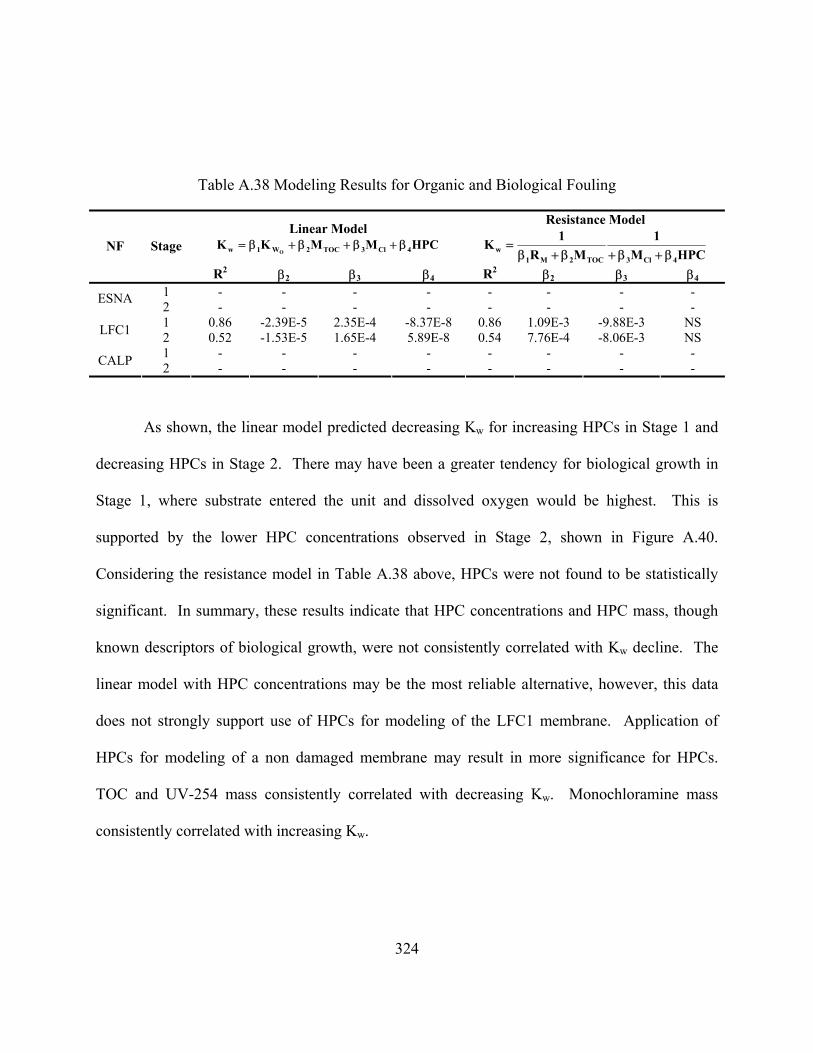
324
Table A.38 Modeling Results for Organic and Biological Fouling
Linear Model Resistance Model
HPCM1
MR1K
4Cl3TOC2M1w β+β+β+β
= HPCMMKK 4Cl3TOC2W1w Oβ+β+β+β= NF Stage
R2 β2 β3 β4 R β2 β3 β4
1 - - - - - - - -
2
ESNA 2 - - - - - - - - 1 0.86 -2.39E-5 2.35E-4 -8.37E-8 0.86 1.09E-3 -9.88E-3 NS LFC1 2 0.52 -1.53E-5 1.65E-4 5.89E-8 0.54 7.76E-4 -8.06E-3 NS 1 - - - - - - - - CALP 2 - - - - - - - -
As shown, the linear model predicted decreasing Kw for increasing HPCs in Stage 1 and
decreasing HPCs in Stage 2. There may have been a greater tendency for biological growth in
Stage 1, where substrate entered the unit and dissolved oxygen would be highest. This is
supported by the lower HPC concentrations observed in Stage 2, shown in Figure A.40.
Considering the resistance model in Table A.38 above, HPCs were not found to be statistically
significant. In summary, these results indicate that HPC concentrations and HPC mass, though
known descriptors of biological growth, were not consistently correlated with Kw decline. The
linear model with HPC concentrations may be the most reliable alternative, however, this data
does not strongly support use of HPCs for modeling of the LFC1 membrane. Application of
HPCs for modeling of a non damaged membrane may result in more significance for HPCs.
TOC and UV-254 mass consistently correlated with decreasing Kw. Monochloramine mass
consistently correlated with increasing Kw.
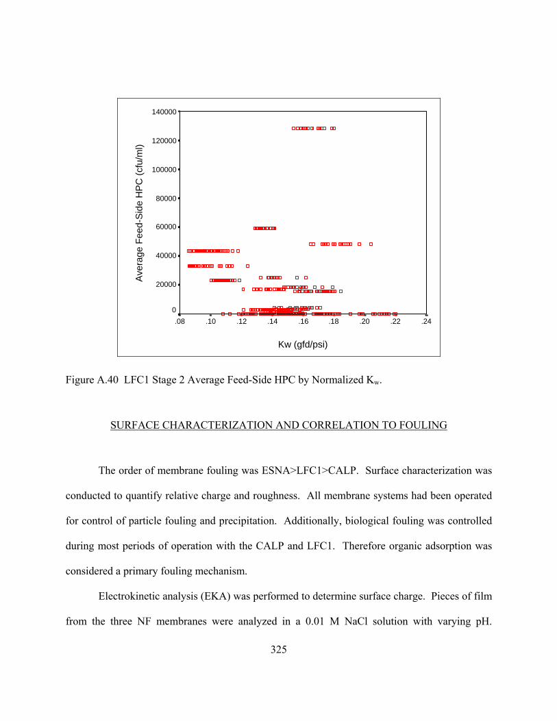
Kw (gfd/psi)
.24.22.20.18.16.14.12.10.08
Ave
rage
Fee
d-S
ide
HP
C (c
fu/m
l)
140000
120000
100000
80000
60000
40000
20000
0
Figure A.40 LFC1 Stage 2 Average Feed-Side HPC by Normalized Kw.
SURFACE CHARACTERIZATION AND CORRELATION TO FOULING
The order of membrane fouling was ESNA>LFC1>CALP. Surface characterization was
conducted to quantify relative charge and roughness. All membrane systems had been operated
for control of particle fouling and precipitation. Additionally, biological fouling was controlled
during most periods of operation with the CALP and LFC1. Therefore organic adsorption was
considered a primary fouling mechanism.
Electrokinetic analysis (EKA) was performed to determine surface charge. Pieces of film
from the three NF membranes were analyzed in a 0.01 M NaCl solution with varying pH.
325
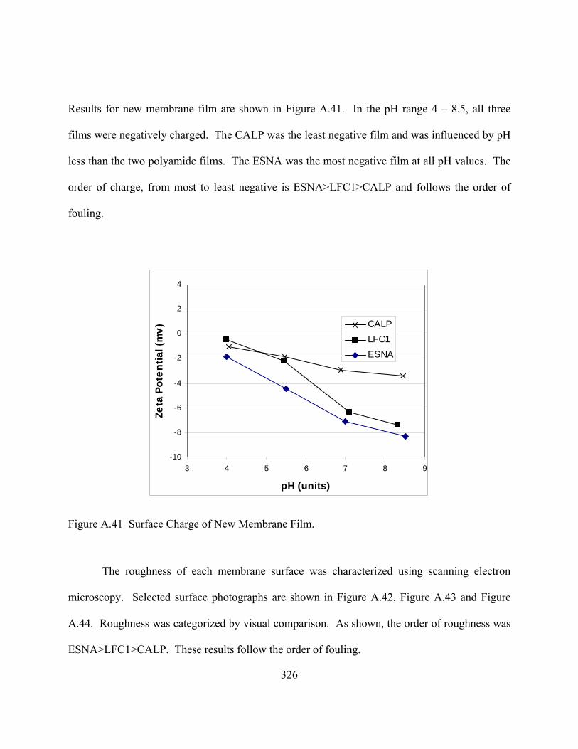
326
Results for new membrane film are shown in Figure A.41. In the pH range 4 – 8.5, all three
films were negatively charged. The CALP was the least negative film and was influenced by pH
less than the two polyamide films. The ESNA was the most negative film at all pH values. The
order of charge, from most to least negative is ESNA>LFC1>CALP and follows the order of
fouling.
-10
-8
-6
-4
-2
0
2
4
3 4 5 6 7 8
pH (units)
Zeta
Pot
entia
l (m
v)
9
CALPLFC1ESNA
Figure A.41 Surface Charge of New Membrane Film.
The roughness of each membrane surface was characterized using scanning electron
microscopy. Selected surface photographs are shown in Figure A.42, Figure A.43 and Figure
A.44. Roughness was categorized by visual comparison. As shown, the order of roughness was
ESNA>LFC1>CALP. These results follow the order of fouling.
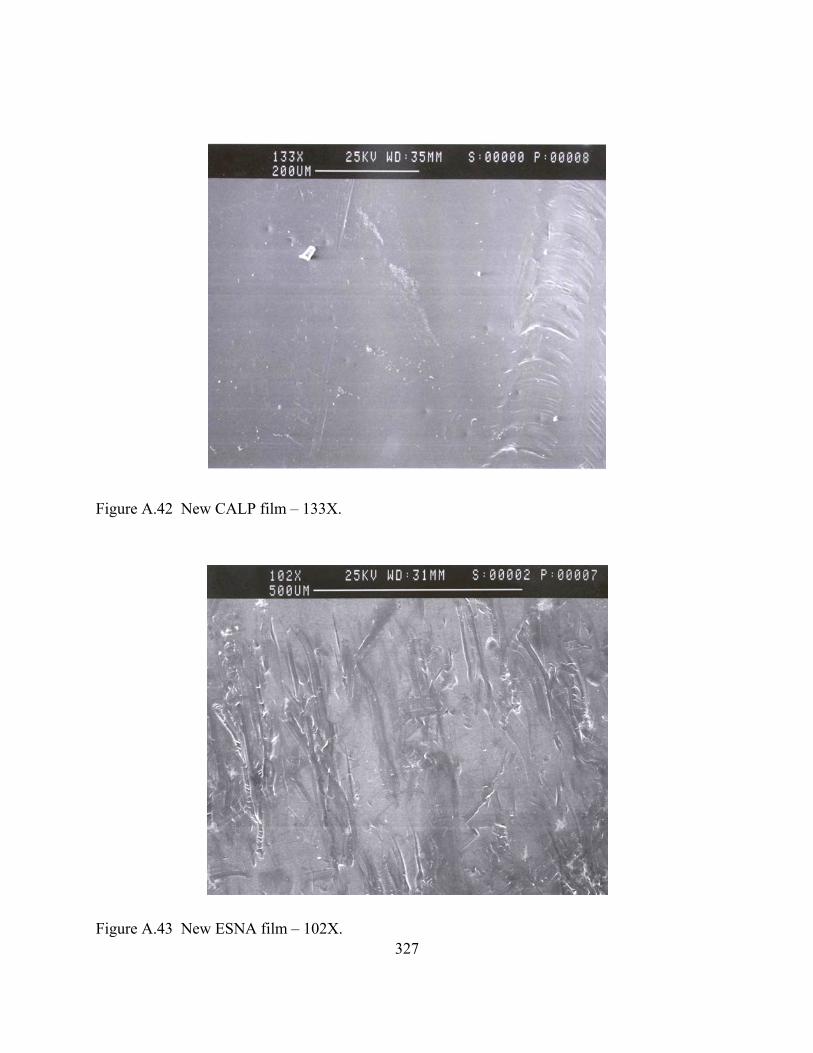
Figure A.42 New CALP film – 133X.
327
– 102X. Figure A.43 New ESNA film

Figure A.44 New LFC1 film – 100X.
The data above indicate fouling increased with increasing roughness and increasingly
negative charge. The ability of more negatively charged polyamide membranes to better reject
natural organic matter has been explained by charge repulsion (Marinas and Selleck, 1992). The
negatively-charged polymeric surface repels like-charged solutes and has a high affinity for
water (hydrophilicity) which also explains the higher productivity of these membranes (Bitter,
1991; Gregor 1976). Additionally, the rejection of a greater quantity of natural organic matter is
expected to reduce adsorptive fouling (Nystrom et al.., 1991, Jucker and Clark, 1994). In fact,
the results of this field study show greater adsorptive fouling for the more negatively charged
polyamide membranes. These results do not support a charge-repulsion mechanism for fouling
control. Other research has found similar results at bench-scale, with less organic fouling for
328

329
cellulose acetate over polyamide membranes (Nilson and DiGiano, 1996). One possible
explanation is a difference in surface area, due to surface roughness. A rougher film will have a
greater number of sites for adsorption or ion exchange. Polymeric membranes are typically
weak ion-exchange membranes with fixed charge groups commonly provided by sulfonic (SO3-)
and carboxylic (COO-) functional groups (Marinas and Selleck, 1992; Demish and Pusch, 1976).
Regardless of the cause, charge-repulsion by the more negatively charged membranes did not
mitigate fouling but instead these membranes experienced higher fouling rates than less
negatively charged membranes, for this research. Surface roughness correlates with fouling and
may be due to the associated increase in surface area and organic adsorption, as opposed to
increased particle fouling.
CONCLUSIONS
• A cellulose acetate nanofilter (CALP) was less susceptible to fouling than two
polyamide nanofilters (ESNA and LFC1). The cellulose acetate nanofilter incurred
less than a 10 percent decline in productivity over 6 months of operation and is a
viable nanofilter for surface water treatment.
• The cellulose acetate nanofilter was susceptible to biological degradation and
required use of a biocide to preserve membrane integrity. Cellulose acetate is a
known biological substrate and use of CA membranes requires more diligent
oversight to ensure integrity is not lost, compared to more chemically stable
polyamide membranes.

330
• One polyamide nanofilter (ESNA) fouled irreversibly and could not be used for this
site. Measures of biological activity were not obtained however biological growth
and organic adsorption are suspected contributors to fouling.
• One polyamide nanofilter (LFC1) suffered from biological fouling; cleaning cycles
were improved with the addition of monochloramine.
• The LFC1 polyamide nanofilter suffered damage due to oxidation from
monochloramine and would need a non oxidative biocide for use at this site. Damage
was quantified via increasing Kw and decreasing TDS rejection.
• Advanced pretreatment processes (CSF, MF, and C/MF) reduced turbidity to less
than 0.3 NTU in the nanofilter feed, which eliminated particle fouling.
• Acid and antiscalent addition controlled precipitation fouling.
• Biological growth and organic adsorption were primary factors that contributed to
nanofilter productivity decline.
• The resistance model for NF productivity was expanded to include terms for
biological, adsorptive, and particle fouling. The model was integrated for a condition
of constant flux and for a condition of constant pressure. For constant flux, NF
productivity is proportional to one over time. For constant pressure, productivity is
proportional to one over the square root of time.
• Regression of the pilot-scale data showed that the linear model fit this data better than
the resistance model.

331
• Due to effective removal of particles by the pretreatment processes, NF particle
plugging did not occur and was not a consistent modeling factor.
• Regression of TOC and UV-254 mass corresponded to decreasing Kw indicating
organic adsorption and/or substrate-limited biological growth were significant factors
in productivity decline. Continued Kw decline in the presence of monochloramine
confirms that organic adsorption was a factor. HPC mass and concentration did not
consistently correlate with Kw decline. However, non-statistical comparisons showed
biological growth to be an important factor; data limitations may have reduced to
significance of the statistical regressions.
• Regression of TOC and UV-254 mass resulted in common conclusions which
indicates UV-254 may be a reliable substitute for the more costly and time consuming
analytical technique associated with TOC.
• The order of membrane fouling, from most to least fouling, was
ESNA>LFC1>CALP.
• The order of membrane surface charge, from most to least negative, as well as surface
roughness, from most to least rough, was ESNA>LFC1>CALP, which followed the
order of fouling.
• A more negatively charged membrane surface correlated with increased fouling,
indicating electrostatic repulsion was not effect for fouling control. Increased surface
area, due to greater surface roughness, for the more negatively charged membranes
may have contributed to organic adsorption fouling. Therefore, with respect to
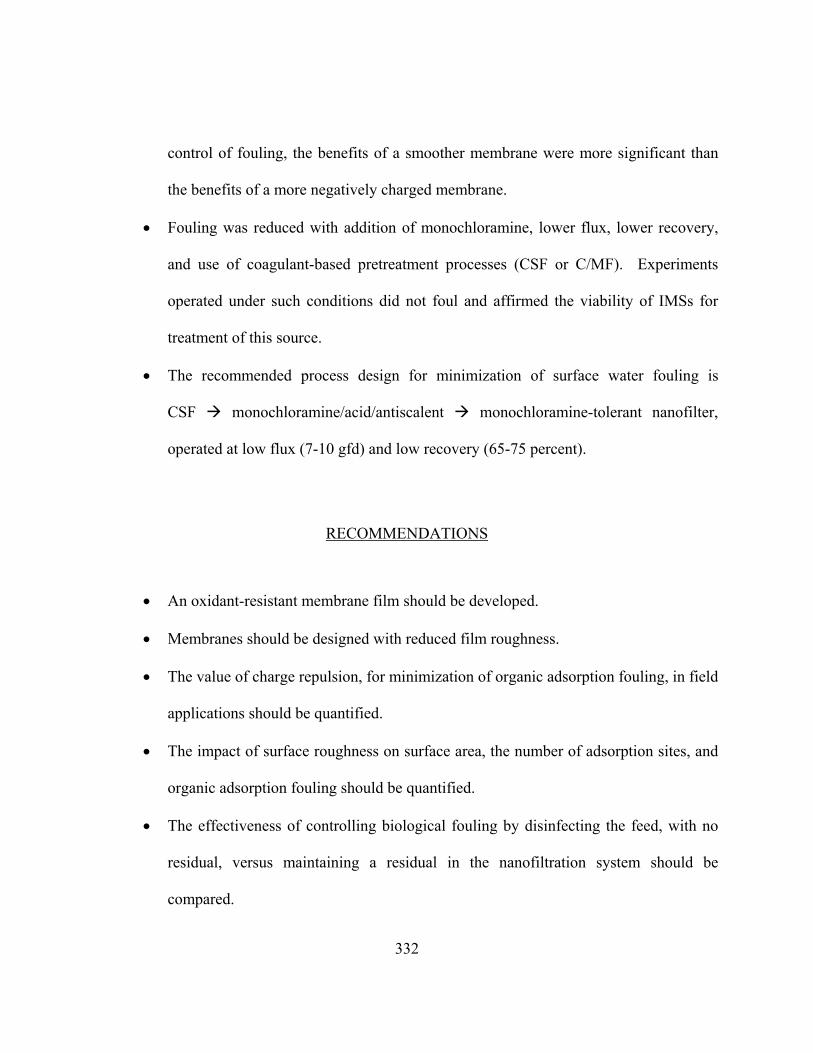
332
control of fouling, the benefits of a smoother membrane were more significant than
the benefits of a more negatively charged membrane.
• Fouling was reduced with addition of monochloramine, lower flux, lower recovery,
and use of coagulant-based pretreatment processes (CSF or C/MF). Experiments
operated under such conditions did not foul and affirmed the viability of IMSs for
treatment of this source.
• The recommended process design for minimization of surface water fouling is
CSF monochloramine/acid/antiscalent monochloramine-tolerant nanofilter,
operated at low flux (7-10 gfd) and low recovery (65-75 percent).
RECOMMENDATIONS
• An oxidant-resistant membrane film should be developed.
• Membranes should be designed with reduced film roughness.
• The value of charge repulsion, for minimization of organic adsorption fouling, in field
applications should be quantified.
• The impact of surface roughness on surface area, the number of adsorption sites, and
organic adsorption fouling should be quantified.
• The effectiveness of controlling biological fouling by disinfecting the feed, with no
residual, versus maintaining a residual in the nanofiltration system should be
compared.

333
• The potential for fouling of the CALP membrane at higher recoveries and in the
presence of high organic concentrations should be investigated by extended
operation, to ensure sufficient productivity decline is observed and reliable fouling
rates are obtained.
• Given the susceptibility of cellulose acetate membranes to biological degradation and
the high HPC counts observed at low monochloramine levels (<1.0 mg/L), higher
(>1.0 mg/L) monochloramine residuals should be utilized for future research.
REFERENCES
Chellam, S., 1995. Laminar Fluid Flow, Particle Transport and Permeate Flux Behavior in Crossflow Membrane Filters, Ph.D. Dissertation, Rice University, Houston, TX.
Chellam, S., Jacangelo, J.G., Bonacquisti, T.P., and Long, B.W., 1997. Effect of Operating Conditions and Pretreatment on Nanofiltration of Surface Water, Proceedings of the Membrane Technology Conference, American Water Works Association, New Orleans, LA, 215-231.
Elimelech, M., Zhu, X., Childress, A.E., and Hong, S., 1997. Role of Membrane Surface Morphology in Colloidal Fouling of Cellulose Acetate and Composite Aromatic Polyamide Reverse Osmosis Membranes, Journal of Membrane Science, 127, 101-109.
Faust, S.D. and Aly, O.M., 1983. Chemistry of Water Treatment, Butterworth Publishers, Stoneham, MA.
Green G. and Belfort G., 1980. Fouling of Ultrafiltration Membranes: Lateral Migration and the Particle Trajectory Model, Desalination, 35.
Mulford, L.A., Tram, Q., and Taylor, J.S., Feb. 1999. “Modeling and Performance Evaluation of a Groundwater Nanofiltration Plant”, Proceedings of the AWWA Membrane Technology Conference, Long Beach, CA.

334
Reiss, C.R. Robert, C. and Taylor, J.S., Feb. 1997. Multi-Contaminant Removal by Integrated Membrane Systems, Proceedings of the Membrane Technology Conference, American Water Works Association, New Orleans, LA, 289-306.
Speth, T.F., Fromme W.R., Summers, R.S., Aug. 1995. Evaluation of Membrane Performance and Fouling by Pyrolysis-GC/MS, Proceedings of the Membrane Technology Conference, American Water Works Association, Reno, NV, 641-663.
Taylor, J.S., 1996. Reverse Osmosis and Nanofiltration, in Water Treatment Membrane Processes, ed. P. Jacobs, et al., McGraw-Hill, NY.
Taylor, J.S., Reiss, C.R., Morris, K.E., Jones, P.S., Smith, D.K., Lyn, T.L. and Duranceau, S.J., Feb. 1992. Reduction of Disinfection By-Product Precursors by Nanofiltration, USEPA Report No. EPA/ 600/ R-92/023.
Weber, W.J. Jr., 1972. Physicochemical Processes for Water Quality Control, John Wiley and Sons, New York, NY.
Top Related