


Languages
Pages
Legal


Mass transfer equation
Migration
Mixed migration & diffusion near an electrodeMass transfer during electrolysisEffect of excess electrolyte
Diffusion Microscopic viewFick’s lawsBoundary conditions in electrochemical problemsSolution of diffusion equations
Mass transfer by migration & diffusion (Ch. 4)

Mass transfer equationMass transfer by diffusion, migration, convection- Diffusion & migration result from a gradient in electrochemical potential, μ- Convection results from an imbalance of forces on the solution
Two points in solution; r & s→ difference of μjdue to conc. & electric field (φ) differences
Flux Jj∝ gradμj or Jj∝∇μj
1-D: ∇ = i(∂/∂x)3-D: ∇ = i(∂/∂x) + j(∂/∂y) + k(∂/∂z)
Jj = -(CjDj/RT)∇μjMinus sign: flux direction opposite the direction of increasing μj
If solution moving with a velocity vJj = -(CjDj/RT)∇μj + Cjv

Nernst-Planck equations
Jj(x) = -Dj(∂Cj(x)/∂x) –(zjF/RT)DjCj(∂φ(x)/∂x) + Cjv(x)
In generalJj = -Dj∇Cj – (zjF/RT)DjCj∇φ + Cjv
diffusion migration convection
Convection absent in this Chapter (Ch.9 for convection)→ in an unstirred or stagnant solution
For linear system-Jj (mols-1cm-2) = ij/zjFA [C/s per (Cmol-1cm2)] = id,j/zjFA + im,j/zjFA
With id,j/zjFA = Dj(∂Cj/∂x)im,j/zjFA = (zjFDj/RT)Cj(∂φ/∂x)
Id,j & im,j: diffusion & migration currents of species j
Total current i = ∑ij

Migration
In the bulk soln (away from the electrode), conc gradient small: migrationij = (zj
2F2ADjCj/RT)(∂φ/∂x)
Einstein-Smoluchowski equationmobility uj FDj/RT׀ zj׀ =
ij FAujCj(∂φ/∂x)׀zj׀ =For a linear electric field
∂φ/∂x = ΔE/l
ij FAujCjΔE/l׀zj׀ =
Total current i = ∑ij = (FAΔE/l)∑ ׀zj ׀ujCj
Conductance (L) L = 1/R = i/ΔE = (FA/l)∑ ׀zj ׀ujCj = Aκ/lκ: conductivity (Ω-1cm-1)
κ = F∑ ׀zj ׀ujCjResistivity ρ = 1/κ
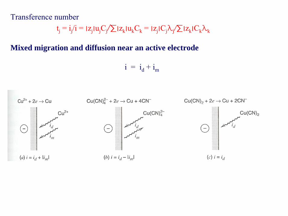
Transference numbertj = ij/i ukCk׀ zk׀ ∑/ujCj׀ zj׀ = Ckλk׀ zk׀ ∑/Cjλj׀ zj׀ =
Mixed migration and diffusion near an active electrode
i = id + im

Balance sheets for mass transfer during electrolysise.g., 4.1. Electrolysis of a solution of HCl at Pt electrode
λ+ (conductance of H+), λ- (conductance of Cl-): λ+ ~ 4λ-→ t+ = 0.8, t- = 0.2Assume total current of 10e/unit time producing 5H2 (cathode) & 5Cl2 (anode)Total current in bulk soln: 8H+ + 2Cl-
→ diffusion of 2 additional H+ to cathode with 2Cl- for electroneutralitydiffusion of 8Cl- with 8H+
For H+: id = 2, im = 8, for Cl-: id = 8, im =2 → total current i = id + im = 10(same direction of id & im)

For mixture of charged species, current by jth species ij = tji→ # of moles of jth species migrating per sec = tji/zjF→ # of moles arriving at the electrode per sec by migration = ±im/nF
(positive sign for reduction of j, negative sign for oxidation)
±im/nF = tji/zjF
im = ±(n/zj)tji
id = i – im = i(1 -/+ ntj/zj)
Negative sign for cathodic current, positive sign for anodic current)

e.g., 4.2. Electrolysis of a solution of 10-3 M Cu(NH3)42+, 10-3 M Cu(NH3)2
+, 3 x 10⁻³ M Cl- in 0.1 M NH3 at two Hg electrodes
Assume λCu(II) = λCu(I) = λCl- = λ
tCu(II) = 1/3, tCu(I) = 1/6, tCl- = 1/2Assume total current of 6e/unit time, i = 6, n = 1 For Cu(II) at cathode: ׀im ׀ = (1/2)(1/3)(6) = 1, id = 6 - 1 = 5, for Cu(I) at anode: ׀im ׀ = (1/1)(1/6)(6) = 1, id = 6 + 1 = 7
From tj = ij/i ukCk׀ zk׀ ∑/ujCj׀ zj׀ = Ckλk׀ zk׀∑/Cjλj׀ zj׀ =
Effect of adding excess electrolytee.g., 4.3. Electrolysis of a solution of 10-3 M Cu(NH3)4
2+, 10-3 M Cu(NH3)2+,
3 x 10⁻³ M Cl- in 0.1 M NH3 + 0.1 M NaClO4 (as excess electrolyte) at two Hg electrodes
Assume λNa+ = λClO4- = λ→ tNa+ = tClO4- = 0.485, tCu(II) = 0.0097, tCu(I) = 0.00485, tCl- = 0.0146*Na+ & ClO4
- do not participate in e-transfer rxns, but because their conc are high, they carry 97% of the current in the bulk solution
→Most of Cu(II) reaches the cathode by diffusion & 0.5% flux by migration
Addition of an excess of nonelectroactive ions (a supporting electrolyte):1. nearly eliminates the contribution of migration to the mass transfer of the electroactive species → eliminate ∇φ or ∂φ/∂x in mass transfer equations
2. Decreases the solution resistance, improve the accuracy of WE potential
Disadvantage: impurities, altered medium


DiffusionA microscopic view-discontinuous source model
Diffusion occurs by a “random walk” process
Probability, P(m, r) after m time units (m = t/τ)
P(m, r) = (m!/r!(m – r)!)(1/2)m
where x = (-m + 2r)l with r = 0, 1,…m

Mean square displacement of the molecule
Δ2 = ml2 =(t/τ)l2 = 2DtD: diffusion coefficient (= l2/2τ), cm2/s (Einstein in 1905)
Root-mean square displacementΔ = √2Dt
→ estimating the thickness of diffusion layere.g., D = 5 x 10⁻⁵ cm2/s: diffusion layer thickness 10-4 cm in 1 ms, 10-3 cm in 0.1
s, 10-2 cm in 10 s

For N0 molecules at the original position at t = 0 → Gaussian distribution laterN(x, t) in a segment Δx wide on x
N(x, t)/N0 = (Δx/2√πDt)exp(-x2/4Dt)
2-D: Δ = √4Dt, 3-D: Δ = √6Dt
Diffusional velocity (vd)vd = Δ/t = (2D/t)1/2
Migration (v = uiE) vs. diffusion (vd)
Einstein-Smoluchowski equationmobility uj FDj/RT׀ zj׀ =
v = ׀zj ׀FDjE/RT (E: electric field strength)
v << vd DiE/(RT/ ׀zi ׀F) << (2Di/t)1/2
rearrange (2Dit)1/2E << 2RT/ ׀zi ׀F
→ voltage drop over length scale of diffusion << 2RT/ ׀zi ׀F : migration negligible

Fick’s laws of diffusionFick’s 1st law: flux ∝ conc gradient
-JO(x, t) = DO(∂CO(x, t)/∂x)
Fick’s 2nd law: change in concentration of O with time∂CO(x, t)/∂t = DO(∂2CO(x, t)/∂x2)
→ solution gives concentration profiles, CO(x, t)

General formulation of Fick’s 2nd law
∂CO/∂t = DO∇2CO

Fig. (a): Planar electrode (linear diffusion equation)∂CO(x, t)/∂t = DO(∂2CO(x, t)/∂x2)
Fig. (b): spherical electrode (hanging Hg drop)∂CO(r, t)/∂t = DO[(∂2CO(r, t)/∂x2) + (2/r)(∂CO(r, t)/∂r)]
Consider O transported purely by diffusion to an electrodeO + ne = R
-JO(0, t) = i/nFA = DO[∂CO(x, t)/∂x]x = 0
Top Related