


Languages
Pages
Legal


. . . . . .
Statement of the problemThe mass at zero case
Strict local martingales
Martingale information of the implied volatility smile
Antoine Jacquier
Department of Mathematics, Imperial College London
Workshop Mathematical Finance Beyond Classical Models
ETH Zurich, September 2015Based on joint works with S. de Marco, C. Hillairet and M. Keller-Ressel.
Antoine Jacquier Martingale information of the implied volatility smile

. . . . . .
Statement of the problemThe mass at zero case
Strict local martingales
Statement of the problem
Consider an (arbitrage-free) implied volatility smile for a given maturity.There exists an underlying stock price process S that generates it.
We wish to answer the following two questions:
(I) Can S describe a defaultable asset?
(II) Is S a true martingale?
ANSWER:
this can ONLY be detected in
(I) the left wing of the smile (small strikes).
(II) the right wing of the smile (large strikes).
Antoine Jacquier Martingale information of the implied volatility smile

. . . . . .
Statement of the problemThe mass at zero case
Strict local martingales
Statement of the problem
Consider an (arbitrage-free) implied volatility smile for a given maturity.There exists an underlying stock price process S that generates it.
We wish to answer the following two questions:
(I) Can S describe a defaultable asset?
(II) Is S a true martingale?
ANSWER: this can ONLY be detected in
(I) the left wing of the smile (small strikes).
(II) the right wing of the smile (large strikes).
Antoine Jacquier Martingale information of the implied volatility smile

. . . . . .
Statement of the problemThe mass at zero case
Strict local martingales
Review of the literatureMain resultsFinancial implications
PART I: MASS AT THE ORIGIN
Joint work with C. Hillairet and S. De Marco
Antoine Jacquier Martingale information of the implied volatility smile
. . . . . .
Statement of the problemThe mass at zero case
Strict local martingales
Review of the literatureMain resultsFinancial implications
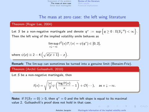
The mass at zero case: the left wing literature.Theorem (Roger Lee, 2004)..
......
Let S be a non-negative martingale and denote q∗ := sup{q ≥ 0 : E(S−q
T ) <∞}
.
Then the left wing of the implied volatility smile behaves as
lim supx↓−∞
I 2(x)T/|x | = ψ(q∗) ∈ [0, 2],
where ψ(z) ≡ 2 − 4(√
z(z + 1) − z)
.
Remark: The lim sup can sometimes be turned into a genuine limit (Benaim-Friz)..Theorem (Archil Gulisashvili, 2010)..
......
Let S be a non-negative martingale, then
I (x) =
√|x |Tψ
(log P(x)
x− 1
)+ O(· · · ), as x ↓ −∞.
Note: if P(ST = 0) > 0, then q∗ = 0 and the left slope is equal to its maximalvalue 2. Gulisashvili’s proof does not hold in that case.
Antoine Jacquier Martingale information of the implied volatility smile
. . . . . .
Statement of the problemThe mass at zero case
Strict local martingales
Review of the literatureMain resultsFinancial implications
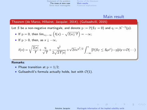
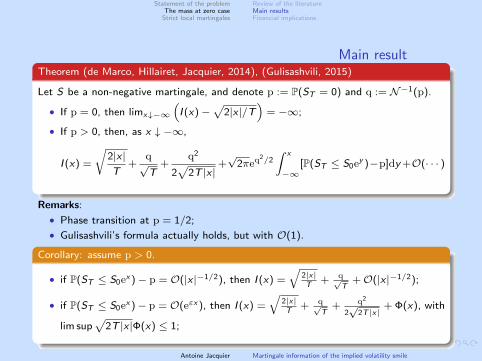
Main result.Theorem (de Marco, Hillairet, Jacquier, 2014), (Gulisashvili, 2015)..
......
Let S be a non-negative martingale, and denote p := P(ST = 0) and q := N−1(p).
• If p = 0, then limx↓−∞
(I (x) −
√2|x |/T
)= −∞;
• If p > 0, then, as x ↓ −∞,
I (x) =
√2|x |T
+q
√T
+q2
2√
2T |x |+√
2πeq2/2∫ x
−∞[P(ST ≤ S0e
y )−p]dy +O(· · · )
Remarks:
• Phase transition at p = 1/2;
• Gulisashvili’s formula actually holds, but with O(1).
.Corollary: assume p > 0...
......
• if P(ST ≤ S0ex ) − p = O(|x |−1/2), then I (x) =
√2|x|T
+ q√T
+ O(|x |−1/2);
• if P(ST ≤ S0ex ) − p = O(eεx ), then I (x) =
√2|x|T
+ q√T
+ q2
2√
2T |x|+ Φ(x), with
lim sup√
2T |x |Φ(x) ≤ 1;
Antoine Jacquier Martingale information of the implied volatility smile
. . . . . .
Statement of the problemThe mass at zero case
Strict local martingales
Review of the literatureMain resultsFinancial implications
Main result.Theorem (de Marco, Hillairet, Jacquier, 2014), (Gulisashvili, 2015)..
......
Let S be a non-negative martingale, and denote p := P(ST = 0) and q := N−1(p).
• If p = 0, then limx↓−∞
(I (x) −
√2|x |/T
)= −∞;
• If p > 0, then, as x ↓ −∞,
I (x) =
√2|x |T
+q
√T
+q2
2√
2T |x |+√
2πeq2/2∫ x
−∞[P(ST ≤ S0e
y )−p]dy +O(· · · )
Remarks:
• Phase transition at p = 1/2;
• Gulisashvili’s formula actually holds, but with O(1)..Corollary: assume p > 0...
......
• if P(ST ≤ S0ex ) − p = O(|x |−1/2), then I (x) =
√2|x|T
+ q√T
+ O(|x |−1/2);
• if P(ST ≤ S0ex ) − p = O(eεx ), then I (x) =
√2|x|T
+ q√T
+ q2
2√
2T |x|+ Φ(x), with
lim sup√
2T |x |Φ(x) ≤ 1;
Antoine Jacquier Martingale information of the implied volatility smile
. . . . . .
Statement of the problemThe mass at zero case
Strict local martingales
Review of the literatureMain resultsFinancial implications
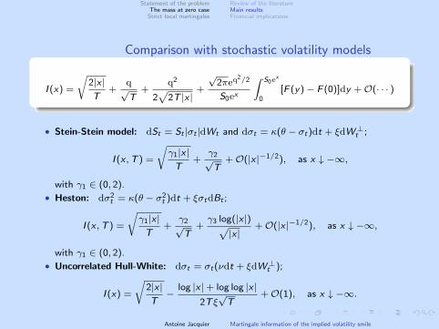
Comparison with stochastic volatility models.
......I (x) =
√2|x |T
+q
√T
+q2
2√
2T |x |+
√2πeq
2/2
S0ex
∫ S0ex
0[F (y) − F (0)]dy + O(· · · )
• Stein-Stein model: dSt = St |σt |dWt and dσt = κ(θ − σt)dt + ξdW⊥t ;
I (x ,T ) =
√γ1|x |T
+γ2√T
+ O(|x |−1/2), as x ↓ −∞,
with γ1 ∈ (0, 2).
• Heston: dσ2t = κ(θ − σ2
t )dt + ξσtdBt ;
I (x ,T ) =
√γ1|x |T
+γ2√T
+γ3 log(|x |)√
|x |+ O(|x |−1/2), as x ↓ −∞,
with γ1 ∈ (0, 2).
• Uncorrelated Hull-White: dσt = σt(νdt + ξdW⊥t );
I (x) =
√2|x |T
−log |x | + log log |x |
2Tξ√T
+ O(1), as x ↓ −∞.
Antoine Jacquier Martingale information of the implied volatility smile
. . . . . .
Statement of the problemThe mass at zero case
Strict local martingales
Review of the literatureMain resultsFinancial implications
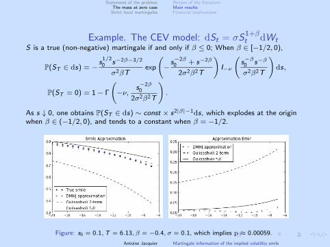
Example. The CEV model: dSt = σS1+βt dWt
S is a true (non-negative) martingale if and only if β ≤ 0; When β ∈ [−1/2, 0),
P(ST ∈ ds) = −s
1/20 s−2β−3/2
σ2βTexp
(−s−2β
0 + s−2β
2σ2β2T
)I−ν
(s−β
0 s−β
σ2β2T
)ds,
P(ST = 0) = 1 − Γ
(−ν,
s−2β0
2σ2β2T
).
As s ↓ 0, one obtains P(ST ∈ ds) ∼ const × s2|β|−1ds, which explodes at the originwhen β ∈ (−1/2, 0), and tends to a constant when β = −1/2.
Figure: s0 = 0.1,T = 6.13, β = −0.4, σ = 0.1, which implies p ≈ 0.00059.
Antoine Jacquier Martingale information of the implied volatility smile
. . . . . .
Statement of the problemThe mass at zero case
Strict local martingales
Review of the literatureMain resultsFinancial implications
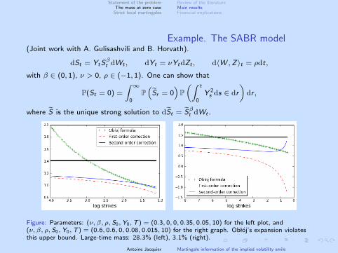
Example. The SABR model(Joint work with A. Gulisashvili and B. Horvath).
dSt = YtSβt dWt , dYt = νYtdZt , d⟨W ,Z⟩t = ρdt,
with β ∈ (0, 1), ν > 0, ρ ∈ (−1, 1). One can show that
P(St = 0) =
∫ ∞
0P(Sr = 0
)P(∫ t
0Y 2s ds ∈ dr
)dr ,
where S is the unique strong solution to dSt = Sβt dWt .
Figure: Parameters: (ν, β, ρ, S0,Y0,T ) = (0.3, 0, 0, 0.35, 0.05, 10) for the left plot, and(ν, β, ρ, S0,Y0,T ) = (0.6, 0.6, 0, 0.08, 0.015, 10) for the right graph. Ob loj’s expansion violatesthis upper bound. Large-time mass: 28.3% (left), 3.1% (right).
Antoine Jacquier Martingale information of the implied volatility smile
. . . . . .
Statement of the problemThe mass at zero case
Strict local martingales
Review of the literatureMain resultsFinancial implications
Financial implications: smile symmetries
• Absence of symmetry: If p = 0, then the smile cannot be symmetric.
• Variance swap prices are infinite: using
1
2E (⟨log(S)⟩T ) =
∫ S0
0
P(K)
K2dK +
∫ ∞
S0
C(K)
K2dK
and limK↓0
P(K)
K= P(ST = 0).
• Gamma swap prices are not impacted (to that extent) by potential default.
Antoine Jacquier Martingale information of the implied volatility smile

. . . . . .
Statement of the problemThe mass at zero case
Strict local martingales
ObservationsPricing and dualityImplied volatility
PART II: STRICT LOCAL MARTINGALES ANDDUALITY
Joint work with M. Keller-Ressel
Antoine Jacquier Martingale information of the implied volatility smile

. . . . . .
Statement of the problemThe mass at zero case
Strict local martingales
ObservationsPricing and dualityImplied volatility
Detecting strict local martingales
Consider a one-dimensional diffusion
dSt = σ(St)dWt , S0 > 0.
.Proposition (Engelbert et al., Mijatovic-Urusov...)..
......
(i) St > 0 almost surely for all t > 0 if and only if
∫ 1
0
z2dz
σ2(z)= ∞;
(ii) S is a strict local martingale if and only if
∫ ∞
1
z2dz
σ2(z)<∞.
Jarrow, Kchia and Protter used (ii) to test whether a given underlying (LinkedIn andgold) was a true martingale or exhibited a bubble. Their approach was based ondevising a statistical procedure to estimate σ() from time series.
Goal here: develop an alternative test, based on the observed implied volatility smile.
Antoine Jacquier Martingale information of the implied volatility smile
. . . . . .
Statement of the problemThe mass at zero case
Strict local martingales
ObservationsPricing and dualityImplied volatility
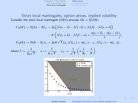
Strict local martingales, option prices, implied volatilityConsider the strict local martingale (CEV) process dSt = S2
t dWt .
CS (K) := E(ST − K)+ = S0
(N (κ− δ) −N (−δ) + N (δ) −N (κ + δ)
)− K
(N (κ + δ) −N (δ − κ) +
n(κ+ δ) − n(κ− δ)
δ
),
PS (K) := E(K − ST )+ = S0K√T (ζ+N (ζ+) + n(ζ+) − ζ−N (ζ−) − n(ζ−)) ,
where δ :=1
S0
√T, κ :=
1
K√T, ζ± :=
1√T
(±
1
S0−
1
K
).
Antoine Jacquier Martingale information of the implied volatility smile
. . . . . .
Statement of the problemThe mass at zero case
Strict local martingales
ObservationsPricing and dualityImplied volatility
Set-up: (S,Q): market model without arbitrage opportunities (NFLVR). S0 = 1.
Notations: K = ex .
Consequences and remarks:
• Martingale defect: m := 1 − EQ(ST ) > 0.
• Put-Call parity fails, in particular CS (x) − PS (x) = 1 − ex −m
• Bounds for CS : (1 − ex −m)+ ≤ CS (x) ≤ 1 −m.
Link with no-arbitrage theory:
• Consider a Call option valued at (1 − ex −m)+. Choose x ≤ log(1 −m), andconstruct the portfolio Long Call, short Stock and m + ex cash.Payoff: m + (ex − ST )+ > 0.Resolution of the ‘paradox’: the short position in S implies that the portfolio isunbounded from below, and hence not admissible in the sense of NFLVR.
Antoine Jacquier Martingale information of the implied volatility smile
. . . . . .
Statement of the problemThe mass at zero case
Strict local martingales
ObservationsPricing and dualityImplied volatility
Pricing with collateral
.Theorem: Cox-Hobson (2005)—simplified..
......
Let G be a positive convex function satisfying lim sups↑∞ s−1G(s) = α and G(s) ≤(s − ex )+. The fair price of a European Call option is EQ(ST − ex )+ + αm =: Cα
S (x).
Note: α represents the amount of collateral the option seller needs to post.Furthermore, limx↑∞ Cα
S (x) = αm and limx↑∞(PαS (x) − ex ) = m− 1.
.Theorem: Madan-Yor (2006)—fully collateralised price α = 1..
......
For any sequence of stopping times (τn)n≥0,
CMYS (x) := lim
n↑∞EQ (ST∧τn − ex )+ = (1 − ex )+ +
1
2EQ(Lx
T ) = CS (x) + πST ,
where (Lxt )t≥0 denotes the local time of S at level ex , and where the penalty term reads
πST = lim
z↑∞zQ
(sup
0≤u≤TSu ≥ z
)= 1 − EQ(ST ) = m.
Antoine Jacquier Martingale information of the implied volatility smile
. . . . . .
Statement of the problemThe mass at zero case
Strict local martingales
ObservationsPricing and dualityImplied volatility
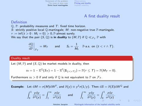
A first duality result
DefinitionQ, P: probability measures and T : fixed time horizon.S: strictly positive local Q-martingale; M: non-negative true P-martingale.τ := inf{t > 0 : Mt = 0} > 0,P-almost surely.We say that the pair (S,Q) is in duality to (M,P) if Q ≪FT
P with
dQdP
∣∣∣∣FT
= MT and St =1
MtP-a.s. on {t < τ ∧ T}.
.Duality result..
......
Let (M,P) and (S,Q) be market models in duality, then
m = 1 − EQ(ST ) = 1 − EP(11{τ>T}) = P(τ ≤ T ) = P(MT = 0).
Furthermore m > 0 if and only if Q is not equivalent to P on FT .
Example: Let dM = σ(M)dW P, and σ(y) ≡ y2σ(1/y). Then dS = σ(S)dWQ and∫ 1
0
ydy
σ2(y)=
∫ ∞
1
zdz
σ2(z)and
∫ ∞
1
ydy
σ2(y)=
∫ 1
0
zdz
σ2(z).
Antoine Jacquier Martingale information of the implied volatility smile

. . . . . .
Statement of the problemThe mass at zero case
Strict local martingales
ObservationsPricing and dualityImplied volatility
Put-Call Duality
.Proposition: Call-Put relationships..
......
Define PM(x) := EP(ex −MT )+ and CM(x) := EP(MT − ex )+. Let (M,P) and (S,Q)be market models in duality. For any α ∈ [0, 1],
CαS (x) = exPM(−x) + (α− 1)m and PS (x) = exCM(−x).
Antoine Jacquier Martingale information of the implied volatility smile
. . . . . .
Statement of the problemThe mass at zero case
Strict local martingales
ObservationsPricing and dualityImplied volatility
Implied volatility: existence
IPS : implied volatility corresponding to the Put price on S (under Q).
IαS : implied volatility corresponding to the α-collateralised Call price on S (under Q).
.Theorem: Existence of implied volatilities..
......
• IPS is well defined on R.
• I 1S ≡ IPS .
• For α ∈ [0, 1), there exists x∗α such that IαS is not well defined on (−∞, x∗α).
• Whenever IαS (x) is well defined, IαS (x) < IPS (x).
Antoine Jacquier Martingale information of the implied volatility smile
. . . . . .
Statement of the problemThe mass at zero case
Strict local martingales
ObservationsPricing and dualityImplied volatility
Implied volatility: asymptotic behaviour
.Theorem: Asymptotic behaviour of the smile (not using duality)..
......
Let S be a strict Q-local martingale with m ∈ (0, 1) and α ∈ (0, 1). As x ↑ ∞,
IαS (x) =
√2x
T+
N−1(αm)√T
+ o(1), and IPS (x) =
√2x
T+
N−1(m)√T
+ o(1).
.Corollary..
......
• If α = 0, then limx↑∞
(I 0S (x) −
√2x
T
)= −∞;
• if m = 0, for α ∈ [0, 1], limx↑∞
(I pS (x) −
√2x
T
)= lim
x↑∞
(IαS (x) −
√2x
T
)= −∞.
Link with Benaim-Friz-Lee: dS = S2dW . p∗ := sup{p ≥ 0 : E(S1+pT ) <∞} = 3, so
that lim sup I (x)2T/x = ψ(p∗) < 2. Benaim-Friz-Lee does not hold in the strict localmartingale case.
Antoine Jacquier Martingale information of the implied volatility smile
. . . . . .
Statement of the problemThe mass at zero case
Strict local martingales
ObservationsPricing and dualityImplied volatility
Duality and implied volatility symmetry.Theorem: Smile symmetry..
......
Let S be a positive strict local Q-martingale in duality with the true P-martingale Mwith mass at zero. Then, for all x ∈ R, I pS (x) = I 1
S (x) = IM(−x). Furthermore, for anyα ∈ (0, 1), IαS cannot be symmetric.
.Theorem: Smile asymptotics refined..
......
S: positive strict local Q-martingale. G(x) := EQ(ST 11{ST≥ex}) and n := N−1(m).
(i) If G(x) = o(x−1/2) as x tends to ∞, then, with 0 ≤ lim supx↑∞ Ψ(x) ≤ 1
I pS (x) = I 1S (x) =
√2x
T+
n√T
+n2
2√
2Tx+
exp( 12n2)
√2Tx
Ψ(x), as x ↑ ∞.
(ii) If G(x) = O(e−εx ) as x tends to ∞, for some ε > 0, then
I pS (x) = I 1S (x) =
√2x
T+
n√T
+n2
2√
2Tx+ Φ(x), as x ↑ ∞,
where lim supx↑∞√
2Tx |Φ(x)| ≤ 1.
Antoine Jacquier Martingale information of the implied volatility smile
. . . . . .
Statement of the problemThe mass at zero case
Strict local martingales
ObservationsPricing and dualityImplied volatility
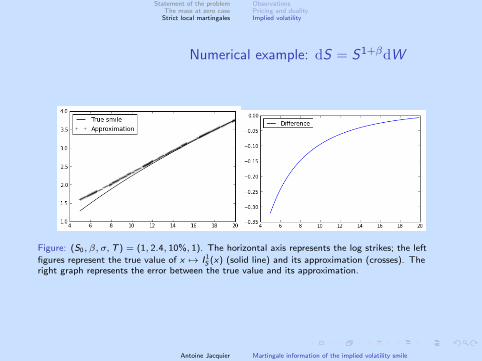
Numerical example: dS = S1+βdW
Figure: (S0, β, σ,T ) = (1, 2.4, 10%, 1). The horizontal axis represents the log strikes; the left
figures represent the true value of x 7→ I 1S (x) (solid line) and its approximation (crosses). The
right graph represents the error between the true value and its approximation.
Antoine Jacquier Martingale information of the implied volatility smile

. . . . . .
Statement of the problemThe mass at zero case
Strict local martingales
ObservationsPricing and dualityImplied volatility
Numerical and practical considerations
• Q: Given observed data, can we construct a rigorous ‘local martingale test’?
• A: Highly dependent on the number of points used to compute the right slope(also liquidity issue...).
• Q: Boundary condition for uniqueness of the corresponding Cauchy problem?
• A: in progress..., see also Ekstrom-Tysk.
• In fact, any test aimed at detecting the strict local martingale property has to beasymptotic; let RT ,x := [0,T ] × (−∞, x), then
sup(t,x)∈RT,x
|PS (x)−PSn (x)| = sup(t,x)∈RT,x
|EQ(ex−ST )+−EQ(ex−SnT )+| ≤ exQ(τn ≥ T ),
where Sn is the stopped true martingale (along the localising sequence).
• Still...warning tool for extrapolation issues: for local-stochastic volatility models(Guyon-Henry-Labordere), arbitrage-free regularisation of SABR..
Antoine Jacquier Martingale information of the implied volatility smile
Top Related