


Languages
Pages
Legal

HAL Id: halshs-00846679https://halshs.archives-ouvertes.fr/halshs-00846679
Submitted on 30 Apr 2015
HAL is a multi-disciplinary open accessarchive for the deposit and dissemination of sci-entific research documents, whether they are pub-lished or not. The documents may come fromteaching and research institutions in France orabroad, or from public or private research centers.
L’archive ouverte pluridisciplinaire HAL, estdestinée au dépôt et à la diffusion de documentsscientifiques de niveau recherche, publiés ou non,émanant des établissements d’enseignement et derecherche français ou étrangers, des laboratoirespublics ou privés.
Market efficiency in the European carbon marketsAmélie Charles, Olivier Darné, Jessica Fouilloux
To cite this version:Amélie Charles, Olivier Darné, Jessica Fouilloux. Market efficiency in the European carbon markets.Energy Policy, Elsevier, 2013, 60, pp.785-792. �10.1016/j.enpol.2013.05.036�. �halshs-00846679�

Market Efficiency in the European Carbon
Markets
Amélie CHARLES∗
Audencia Nantes, School of Management
Olivier DARNɆ
LEMNA, University of Nantes
Jessica FOUILLOUX‡
CREM, University of Rennes 1
∗Audencia Nantes, School of Management, 8 route de la JoneliÃlre, 44312 Nantes, France. Email:
[email protected].†Corresponding author: LEMNA, University of Nantes, IEMN–IAE, Chemin de la Censive du
Tertre, BP 52231, 44322 Nantes, France. Tel: +33 (0)2 40 14 17 33. Fax: +33 (0)2 40 14 16 50.
Email: [email protected].‡University of Rennes 1, 11 rue Jean MacÃl’, CS 70803, 35708 Rennes Cedex 7, France. Email:
1
Abstract
In this paper, we study the relationship between futures and spot prices in
the European carbon markets from the cost-of-carry hypothesis. The aim is to
investigate the extent of efficiency market. The three main European markets
(BlueNext, EEX and ECX) are analyzed during Phase II, covering the period
from March 13, 2009 to January, 17, 2012. Futures contracts are found to be
cointegrated with spot prices and interest rates for several maturities in the three
CO2 markets. Results are similar when structural breaks are taken into account.
According to individual and joint tests, the cost-of-carry model is rejected for all
maturities and CO2 markets, implying that neither contract is priced according
to the cost-of-carry model. The absence of the cost-of-carry relationship can be
interpreted as an indicator of market inefficiency and may bring arbitrage oppor-
tunities in the CO2 market.
Keywords: CO2 emission allowances; Cost-of-carry model; Spot and futures
prices; Market efficiency.
JEL Classification: G13; G14; Q50; C32.
2

Market Efficiency in the European Carbon Markets
Abstract : In this paper, we study the relationship between futures and spot prices in
the European carbon markets from the cost-of-carry hypothesis. The aim is to inves-
tigate the extent of efficiency market. The three main European markets (BlueNext,
EEX and ECX) are analyzed during Phase II, covering the period from March 13, 2009
to January, 17, 2012. Futures contracts are found to be cointegrated with spot prices
and interest rates for several maturities in the three CO2 markets. Results are similar
when structural breaks are taken into account. According to individual and joint tests,
the cost-of-carry model is rejected for all maturities and CO2 markets, implying that
neither contract is priced according to the cost-of-carry model. The absence of the
cost-of-carry relationship can be interpreted as an indicator of market inefficiency and
may bring arbitrage opportunities in the CO2 market.
Keywords: CO2 emission allowances; Cost-of-carry model; Spot and futures prices;
Market efficiency.
JEL Classification: G13; G14; Q50; C32.
3

1 Introduction
The European Union Emission Trading Scheme (EU ETS) went into effect on January
2005, considering the EU Directive 2003/87/EC. The EU ETS is one of the most
important initiatives taken to reduce the greenhouse gas (GHG) emissions (primarily
CO2) that cause climate change (Kyoto protocol). The inclusion of the aviation sector
from January 1st 2012 onwards represents a new step in the implementation of the EU
ETS.1 Following the steady expansion of the EU ETS’ scope to new Member States
since 2005, the European Commission is now adding around 5,000 European airline
companies and foreign companies that do business in Europe to the 11 500 industrial
and manufacturing participating installations. In 2010, it is estimated that the sources
to which the trading scheme applies account for 45 per cent of CO2 emissions and a
little less than 40 per cent of total GHG emissions in that year.
The EU ETS introduces a cap-and-trade system, which operates through the
creation and distribution of tradable rights to emit, usually called EU allowances
(EUAs)2 to installations. Since a constraining cap creates a scarcity rent, these EUAs
have value. The distribution of these rights for free is called free allocation and is the
unique feature of this cap-and-trade system. The cap-and-trade scheme operates over
discrete periods, with the first or pilot period (Phase I, 2005-2007) and with the second
period corresponding to the first commitment period of the Kyoto Protocol. This period
extends from 2008 to 2012 (Phase II) and will be followed by a third period from
1To improve the fluidity of the EU ETS, organized allowance trading has been segmented across
trading platforms: Nordic Power Exchange (Nord Pool) in Norway began in February 2005, European
Energy Exchange (EEX) in Germany began in March 2005, European Climate Exchange (ECX) based
in London and Amsterdam started in April 2005, BlueNext in France and Energy Exchange Austria
(EEA) in Austria began in June 2005, and SendeCO2 in Spain started at the end of 2005.2In fact, the EUAs are the conversion of Assigned Amount Units (AAUs), which are the permits
allocated to Annex B of the Kyoto Protocol. See Convery (2009) and Chevallier (2012) for a discussion
of the EU ETS.
4

2013 to 2020 (Phase III). Phase II represents the fundamental regulatory tool allowing
Member States to reach their Kyoto target. The EU target is a reduction of 8 per
cent below 1990 emissions in the 2008-2012 period.3 To help countries in achieving
their reduction objectives, the Protocol includes three flexibility mechanisms: The
creation of an International Emission Trading, Joint Implementation and the Clean
Development Mechanism.4
The EU ETS includes spot, futures, and option markets with a total market value
of e72 billion in 2010. Futures contracts account for a wide part of this value (about
87% in 2010). Understanding the relationship between spot and futures prices is thus
of crucial importance for all participants in the carbon market. Carbon trading works
only if markets for carbon provide enough liquidity and pricing accuracy, i.e., markets
provide prices that are useful for hedgers and other users of carbon markets. The
efficiency of the CO2 market is particularly important for emission intensive firms,
policy makers, risk managers and for investors in the emerging class of energy and
carbon hedge funds (see Krishnamurti and Hoque, 2011).
Although relevant papers have been published on the behavior of emission
allowance spot and futures prices (see, e.g., Alberola et al., 2008; Daskalakis and
3Phase III is set to help meet the European target of 20 per cent GHG emission reduction in 2020
compared to 1990, in line with the objective of the Climate Energy Package approved in December
2008.4The Joint Implementation (JI) mechanism consists of the realization of an emission reduction
project by a developed country (Annex I country) in another developed country (Annex I). JI projects
provide for Emission Reduction Units (ERUs) that may be utilized by an Annex I country promoting
the project to meet its emission targets under the Kyoto Protocol. The Clean Development Mechanism
(CDM) provides for a similar mechanism for an Annex I country to achieve its emissions target when
the project is implemented in a developing country. The units arising from such projects are termed
Certified Emission Reduction units (CERs). In 2011, the volume of transactions amounted to 6,053
million EUAs, 1,418 million CERs and 62.8 million ERUs (up 20%, 53% and 1,406%, respectively,
compared with 2010).
5

Markellos, 2008; Paolella and Taschini, 2008; Seifert et al., 2008; Benz and Trück,
2009), studies on CO2 market efficiency between futures and spot prices are rather
sparse (Daskalakis et al., 2009; Uhrig-Homburg and Wagner, 2009; Joyeux and
Milunovich, 2010). These studies examine the extent of market efficiency in the
CO2 futures market by conducting empirical tests of the cost-of-carry model, which
allow to ascertain the degree to which carbon futures prices reflect their theoretical
(no arbitrage) values. This approach is especially useful in the context of examining
whether futures contracts are efficiently priced with respect to the underlying emission
rights allowances. If these contracts are efficiently priced then participating countries
and covered installations in them can achieve environmental compliance in a cost-
effective and optimal manner (Krishnamurti and Hoque, 2011).
The aim of this paper is to investigate the efficiency hypothesis between spot
and futures prices negotiated on European markets from a cost-of-carry model,
by extending the previous studies in three ways: (i) we study the three main
European markets, BlueNext, European Energy Exchange (EEX), and European
Climate Exchange (ECX); (ii) we consider the second trading period (Phase II)
from March 13, 2009 to January, 17, 2012; and (iii) we test the cost-of-carry model
using four futures contracts (December 2009, December 2010, December 2011
and December 2012 maturities). This study should give a more complete picture
of the relationships between spot and futures prices in the EU ETS. We apply the
cointegration methodology developed by Johansen (1988, 1991) to test for multivariate
cointegration between the series (futures prices, spot prices and interest rate) before
estimating the cost-of-carry relationship. Indeed, the theoretical connection between
spot and futures prices is a long-run, rather than short-run, concept. In the short-
run, there might be deviations between spot prices and futures prices, that can be
induced by, for example, thin trading or lags in information transmission (Maslyuk
and Smyth, 2009). The visual inspection of the data in Figures 1-3 reveals a sharp
6
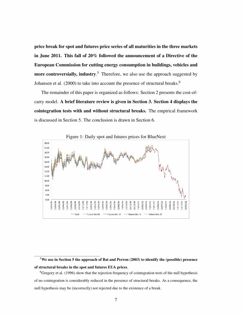
price break for spot and futures price series of all maturities in the three markets
in June 2011. This fall of 20% followed the announcement of a Directive of the
European Commission for cutting energy consumption in buildings, vehicles and
more controversially, industry.5 Therefore, we also use the approach suggested by
Johansen et al. (2000) to take into account the presence of structural breaks.6
The remainder of this paper is organized as follows: Section 2 presents the cost-of-
carry model. A brief literature review is given in Section 3. Section 4 displays the
cointegration tests with and without structural breaks. The empirical framework
is discussed in Section 5. The conclusion is drawn in Section 6.
Figure 1: Daily spot and futures prices for BlueNext
5We use in Section 5 the approach of Bai and Perron (2003) to identify the (possible) presence
of structural breaks in the spot and futures EUA prices.6Gregory et al. (1996) show that the rejection frequency of cointegration tests of the null hypothesis
of no cointegration is considerably reduced in the presence of structural breaks. As a consequence, the
null hypothesis may be (incorrectly) not rejected due to the existence of a break.
7

Figure 2: Daily spot and futures prices for EEX
Figure 3: Daily spot and futures prices for ECX
2 The cost-of-carry model
Theoretically, if spot and futures markets operate efficiently and are frictionless,
futures contracts should be traded at a price known as the fair value (the Law of One
8

Price). The starting point of most studies is the arbitrage free or cost-of-carry model
in which the futures price is represented as
Ft = Ste(r+u−y)(T−t) (1)
where Ft is the futures price at time t; St is the spot price at time t; r is the risk-free
interest rate; u is the storage cost ; y is either a dividend yield in the case of a dividend
paying stock or a convenience yield in the case of commodity; and T is the expiration
date of the futures contract, and (T − t) is the time to expiry of the futures contract.
The storage costs for CO2 allowances are nil because they only exist on a companies’
balance sheet. Taking logarithms of both sides of Equation (1) gives
Ln(Ft) = Ln(St)+(r− y)(T − t) (2)
Various approaches are possible to determine term structure by using alternative model
specifications for the convenience yield term. Nevertheless, there is no consensus
about the state of futures prices (backwardation, normal backwardation, contango and
normal contango).7 The different possible states of the CO2 emissions market for
each maturity is given in Table 1. As in Borak et al. (2006), the futures of the three
markets appear to be in contango, whatever the maturity. Considering Kaldor (1939),
the convenience yield appears as a way to explain backwardation, a situation where the
7The futures market is said to exhibit backwardation when the futures price Ft,T is less or
equal the current spot price St , it exhibits normal backwardation when the futures price is less or
equal the expected spot price Et(ST ) in T . On the other hand the term (normal) contango is used
to describe the opposite situation, when the futures price Ft,T exceeds the (expected) spot price
in T (Borak et al., 2006). In others words, backwardation and contango are used to describe the
relationship between current spot prices and futures prices whereas normal backwardation and
normal contango are used for the relationship between expected spot prices and futures price.
The idea of normal backwardation and normal contango was initially suggested by Keynes (1930)
and Hicks (1946).
9

futures price is lower than the spot price. Consequently, in this paper we will consider
a cost and carry model with zero convenience yield
Ln(Ft) = Ln(St)+ r(T − t) (3)
This equation suggests a long-term relationship between the series.8 The term (T − t)
in the brackets represents a reverse time trend that starts at T years to contract maturity,
and ends at zero as t approaches T .
In order to test the cost-of-carry model empirically, we re-specify Equation (3) as
Ln(Ft) = αLn(St)+βr(T − t)+ εt (4)
where εt is a white noise error term. Simple empirical tests of the efficiency hypothesis
are based on the following single and joint hypothesis tests: H0 : α = 1, H0 : β = 1, and
H0 : α = β = 1, meaning the restrictions implied by the cost-of-carry model.9 Failure
to reject the joint hypothesis implies that the cost-of-carry hypothesis is not rejected,
suggesting an efficiency of the market. In a perfectly efficient and frictionless market,
the pricing relationship expressed in Equation (2) should hold at every instant over a
futures contract life (Stoll and Whaley, 1990). However, as underlined by Joyeux and
Milunovich (2010), in the presence of market frictions, such as transaction costs and
order execution lags, the no-arbitrage condition should hold in the long run but not
necessarily in the short term.
3 Brief literature survey
Few studies examine the extent of market efficiency in the CO2 futures market by
conducting empirical tests of the cost-of-carry model, which allow to ascertain the
degree to which carbon futures prices reflect their theoretical (no arbitrage) values.8Asymptotic inference concerning just identified cointegrating vectors can be conducted as if they
were Gaussian, provided parameters are estimated by the maximum likelihood procedure.9The joint test is more powerful than the individual tests.
10

Tabl
e1:
Futu
res
mar
kets
ituat
ions B
lueN
ext
Dec
09D
ec10
Dec
11D
ec12
Bac
kwar
datio
nF t
,T≤
S t19
190
0
Nor
mal
back
war
datio
nF t
,T≤
S ter(
T−
t)30
646
0
Con
tang
oF t
,T>
S t16
442
455
655
6
Nor
mal
cont
ango
F t,T>
S ter(
T−
t)15
537
955
055
6
EE
X
Dec
09D
ec10
Dec
11D
ec12
Bac
kwar
datio
nF t
,T≤
S t15
234
0
Nor
mal
back
war
datio
nF t
,T≤
S ter(
T−
t)23
5418
0
Con
tang
oF t
,T>
S t17
142
169
973
6
Nor
mal
cont
ango
F t,T>
S ter(
T−
t)16
339
068
573
6
EC
X
Dec
09D
ec10
Dec
11D
ec12
Bac
kwar
datio
nF t
,T≤
S t42
11
0
Nor
mal
back
war
datio
nF t
,T≤
S ter(
T−
t)47
111
32
Con
tang
oF t
,T>
S t15
445
771
573
6
Nor
mal
cont
ango
F t,T>
S ter(
T−
t)14
944
771
570
4
Not
es:
fore
ach
poss
ible
stat
es,w
eco
mpu
te(i
)the
num
bero
ftim
esw
here
futu
res
pric
esar
ebe
low
oreq
ualt
oth
esp
otpr
ices
and
(ii)
the
num
bero
ftim
esw
here
futu
res
pric
esis
high
erth
anth
e
spot
pric
es.
11

Daskalakis et al. (2009) developed an empirically and theoretically valid framework
for the pricing and hedging of intra-phase and inter-phase futures and options on
futures, respectively, on ECX and Nordpool. In the case of EUA futures, only
intra-phase contracts (December 2006 and December 2007) are found to be well
described by the cost-of-carry model with zero convenience yields. For interphase
futures (December 2008 and December 2009), although the cost-of-carry model is
still applicable, a stochastic, mean reverting convenience yield is needed for accurate
pricing. Uhrig-Homburg and Wagner (2009) use a cost-of-carry model with implied
yields for spot prices on Bluenext, and December 2006, December 2007 and
December 2008 futures prices on ECX. They find obvious arbitrage possibilities
in the market during the year 2005. Empirical evidence suggests that after December
2005, spot and futures prices are linked by the cost-of-carry approach within the first
trading period. Temporary deviations from this linkage may exist but generally vanish
after only a few days. Moreover, these authors show that the CO2 futures market leads
the price discovery process. Joyeux and Milunovich (2010) investigate the relationship
between spot prices on Bluenext, and December 2006 and December 2007 futures
prices on ECX during Phase I over the period of June 2005 to December 2007. They
reject the cost-of-carry hypothesis (without costs of storage and without convenience
yield) for the entire period but find some evidence of improvement in market efficiency
over the period using recursive estimates of the cost-of-carry parameters.
4 Econometric methodology
As the test of cost-of-carry model involves estimation of the cointegrating regression
(i.e. a long-term relationship between the series), it is first relevant to test for
cointegration between the series (futures prices, spot prices and interest rate) before
estimating the cost-of-carry relationship.
12

4.1 Cointegration tests
In order to conduct cointegration tests, we first estimate a vector-autoregressive (VAR)
model on log series. The VAR(p) model is defined as
Yt = A1Yt−1 + · · ·+ApYt−p + εt
where Yt is a vector of non-stationary variables, εt is innovation vector. The lag length,
noted p, of the VAR(p) is determined from the criteria discussed in Lütkepohl (1991)
to determine the lag length.10 Then, we implement the Johansen maximum likelihood
procedure (Johansen, 1988, 1991). This approach consists in estimating a Vector
Error Correction Model (VECM) by maximum likelihood, under various assumptions
about the trend or intercept parameters and the number r of cointegrating vectors, then
conducting likelihood ratio tests. We re-write a p-dimensional VECM as follows
∆Yt =p−1
∑i=1
Γi∆Yt−i +ΠYt−1 + εt (5)
where ∆ is a difference operator, Π = ∑pi=1 Ai− Im, the matrices Γi = −∑
pj=i+1 A j
contain information on the short-run adjustment coefficients of the lagged differenced
variables, the expression ΠYt−1 indicates the error correction term, i.e. it includes the
long-run relationships between the time series.
Johansen (1995) considers five restrictions on the deterministic components. In model
1 the level data Yt have no deterministic trends and the cointegrating equations do not
have intercepts, giving the most restrictive specification. In model 2 the level data Yt
have no deterministic trends and the cointegrating equations have intercepts. In model
3 the level data Yt have linear trends but the cointegrating equations have only inter-
cepts. In model 4 the level data Yt and the cointegrating equations have linear trends.
In model 5 the level data Yt have quadratic trends and the cointegrating equations have
linear trends, giving the least restrictive specification. These five cases are nested from10Results are not given to save space but they are available from the authors upon request.
13

the most restrictive (model 1) to the least restrictive (model 5).
Since it is rare that the deterministic specification is well known a priori, Johansen
(1995) suggests a procedure to determine jointly the co-integration rank and the de-
terministic components of the model. The procedure is based on the so-called Pantula
(1989) principle:11 Start from the most restrictive model and then compare the rank
test statistic with the chosen quantile of the corresponding table. If the model is re-
jected, continue to the model that restricts the constant to the cointegration space. If
this model is also rejected, go to the model with an unrestricted constant. In the case of
rejection, proceed to the model with linear trends in the variables and the cointegration
space. If this is also rejected, repeat the procedure for the next rank. Continue until the
null hypothesis cannot be rejected for the first time.
Johansen (1988, 1991) proposes to use the trace test 12 which is based on the log-
likelihood ratio
LR(r|k) = −Tk
∑i=r+1
ln(1−λi)
where λi is the eigenvalue ranked at the i order, k is the number of endogenous
variables, and r = k− 1, . . . ,1,0. This LR statistic tests the null hypothesis of r
cointegrating relations against the alternative of k cointegrating relations, where k is
the number of endogenous variables, for r = 0,1, . . . ,k−1.
11We suggest the use of the Pantula (1989) principle as a simple and practical way to simultaneously
determine the co-integration rank and the deterministic components of a co-integration model.12Based on simulation experiences, Lutkepohl et al. (2001) show that the trace test display better
properties that the maximum eigenvalue test.
14

4.2 Cointegration tests with structural breaks
One way for testing the multivariate cointegration in the presence of structural breaks
is the approach developed by Johansen et al. (2000) which generalized the Johansen
(1988) maximum likelihood cointegration test in order to include up to two known
breaks. These authors extend the standard VECM with a number of additional
variables in order to account for q exogenous breaks in the levels and trends of the
deterministic components of a vector-valued stochastic process. Specifically, Johansen
et al. (2000) describe the model as follows
∆Yt = α
(β
γ
)′+
(Yt−1
tEt
)+µEt +
p−1
∑i=1
Γi∆Yt−i +p
∑i=1
q
∑ν=1
κν,iDν,t−i + εt (6)
where Yt is a vector of non-stationary variables, ∆ is a difference operator, t = 1, . . . ,T
represents the number of sample periods being q with, as an example, a length
Tν−Tν−1; µ = (µ1 . . .µq); γ = (γ′1 . . .γ′q)′; Dν,t equals 1 for t = Tν−1 and 0 otherwise;
Et =(E1t . . .Eqt)′ for Eνt =∑
Tν−Tν−1i=p+1 Dν,t−1 which is equal to 1 for Tν−1+ p+16 t 6 Tν
and 0 otherwise. Dν,t−1 can be considered as an indicator function for the ith
observation in the νth period while Eνt covers the sample for the νth period.
5 Empirical results
The study sample consists of the daily closing prices of spot EUA prices and futures
EUA prices of maturity December 2009, December 2010, December 2011 and
December 2012, covering the period March 13, 2009 to January 17, 2012, both prices
negotiated on BlueNext, ECX and EEX.13 The data on Euribor zero curve swap interest
rates are obtained from Thomson Financial Datastream. In order to match the interest13Data are available on www.bluenext.fr, www.eex.com and www.theice.com.
15
rate maturity to the maturity of the futures contracts effectively, that is, track the futures
contracts through time, we interpolate the interest rates to monthly maturities within
the data sample. The formula used is the Taylor Young formula at the first order for an
x horizon time, t < x < t +1, and rx the corresponding interest rate
rx = rt+1 +(x− t)(rt+1− rt)/(t +1− t)
Table 2 presents summary statistics for the returns calculated as the first differ-
ences in the logs of the EUA spot prices, futures prices and interest rate, for the three
markets. All the returns are highly non-normal, i.e. showing evidence of significant
negative skewness and excess kurtosis, as might be expected from daily log-returns,
except for the spot and futures log-returns relative to the December 2009 maturity.
The kurtosis coefficient is significant, implying that the distribution of the log-returns
is leptokurtic (i.e., fat-tailed distribution) and thus the variance of the CO2 prices is
principally due to infrequent but extreme deviations. The skewness coefficient is neg-
ative and significant for the spot and futures log-returns, implying that there is more
negative log-returns than positive log-returns. This result means that the distribution of
the spot and futures price changes is asymmetric. The Lagrange Multiplier test for the
presence of the ARCH effect clearly indicates that the log-returns show strong condi-
tional heteroscedasticity, which is a common feature of financial data. In other words,
there are quiet periods with small price changes and turbulent periods with large oscil-
lations.
Prior to testing for cointegration, non-stationarity must be established. We apply
various unit root tests with and without structural breaks on all the series and find that
all of them are characterized by a unit root. When tests are applied on series in first-
difference, they are found to be stationary.14 In other words, all series are integrated
14All results are available upon request to the authors.
16

Table 2: Statistical analysis of log-returns seriesData Obs. Mean (%) SD Skewness Kurtosis ARCH(10)
Bluenext
Spot09 data 184 0.0583 0.0245 -0.2165∗ 3.0680 18.99∗
Dec09 Futures data 184 0.0347 0.0237 -0.1596∗ 2.9140 23.60∗
Interest rate (matching Dec09) 184 -1.1873 0.01884 -0.6548∗ 7.9922∗ 95.15∗
Spot10 data 442 0.0526 0.0210 -0.3201∗ 3.8876∗ 39.75∗
Dec10 Futures data 442 0.0330 0.0203 -0.3123∗ 4.1396∗ 36.52∗
Interest rate (matching Dec10) 442 -0.8847 0.0209 -0.1956 7.3153∗ 50.52∗
Spot11 data 555 0.0628 0.0196 -0.2694∗ 4.4260∗ 56.58∗
Dec11 Futures data 555 0.0385 0.0186 -0.2953∗ 4.6521∗ 52.81∗
Interest rate (matching Dec11) 555 -0.3077 0.0191 0.4021∗ 4.5059∗ 20.65∗
Spot12 data 555 0.0628 0.0196 -0.2694∗ 4.4260∗ 56.58∗
Dec12 Futures data 555 0.0331 0.0182 -0.3066∗∗ 4.7308∗ 49.03∗
Interest rate (matching Dec12) 555 -0.3077 0.0191 0.4022∗ 4.5059∗ 20.65∗
EEX
Spot09 data 185 0.0536 0.0239 -0.2456∗ 3.1821 27.14∗
Dec09 Futures data 185 0.0367 0.0233 -0.1798∗ 3.0061 21.82∗
Interest rate (matching Dec09) 185 -1.9061 0.0337 -2.6590∗ 13.8539∗ 114.80∗
Spot10 data 443 0.0471 0.0202 -0.3899∗ 4.4963∗ 45.00∗
Dec10 Futures data 443 0.0314 0.0200 -0.3620∗ 4.1987∗ 30.47∗
Interest rate (matching Dec10) 443 -0.8805 0.0239 -0.8368∗ 7.3997∗ 113.72∗
Spot11 data 702 -0.0512 0.0201 -0.3443∗ 4.8755∗ 55.79∗
Dec11 Futures data 702 -0.0716 0.0204 -0.4661∗ 4.9856∗ 77.60∗
Interest rate (matching Dec11) 702 -0.5817 0.0195 0.0209 5.7731∗ 96.62∗
Spot12 data 735 -0.0829 0.0231 0.3547∗∗ 9.9074∗ 62.47∗
Dec12 Futures data 735 -0.1084 0.0225 0.2245∗ 10.3895∗ 62.10∗
Interest rate (matching Dec12) 735 -0.2775 0.0206 -0.0470 4.7737∗ 49.15∗
ECX
Spot09 data 195 0.0903 0.0242 -0.1812∗ 3.1521 15.16
Dec09 Futures data 195 0.0802 0.0241 -0.1637∗ 2.9240 13.28
Interest rate (matching Dec09) 195 -2.1639 0.0472 -4.5357∗ 31.0675∗ 124.59∗
Spot10 data 457 0.0313 0.0209 -0.2723∗ 4.0796∗ 39.86∗∗
Dec10 Futures data 457 0.0148 0.0208 -0.2329∗ 3.8193∗ 38.41∗
Interest rate (matching Dec10) 457 -1.1079 0.0261 -2.4570 22.8679 310.78∗
Spot11 data 715 -0.0764 0.0223 -0.4494∗ 4.7731∗ 90.89∗
Dec11 Futures data 715 -0.0963 0.0219 -0.4567∗ 4.6820∗ 96.50∗
Interest rate (matching Dec11) 715 -0.7444 0.0243 -2.6032∗ -2.6032∗ 567.70∗
Spot12 data 735 -0.0848 0.0241 0.2777∗ 10.5063∗ 70.04∗
Dec12 Futures data 735 -0.1095 0.0233 0.2155∗ 10.2357∗ 76.14∗
Interest rate (matching Dec12) 735 -0.2775 0.0206 -0.0377 4.7582∗ 49.22∗
Notes: The skewness and kurtosis statistics are standard-normally distributed under the null of normality distributed returns.
ARCH(10) indicates the Lagrange multiplier test for conditional heteroscedasticity with 10 lags. ∗ means significant at the 5%
level.
17
of order 1.
To identify the (possible) presence of structural breaks in the spot and futures EUA
prices, we use the approach of Bai and Perron (2003). Two breaks are identified in
December 21, 2009, and in June 24, 2011. The first break can be explained by the
correlation between the natural gas and carbon markets. Since October 2009, the re-
lationship between natural gas, coal and carbon prices seems to have returned. With
prices of coal rising (by 4% in December) more than those of natural gas, the CO2
switch price dipped further below CO2 market price, providing an incentive for power
producers to switch from coal to gas. Lower demand for CO2 allowance resulting
from this switch (burning gas emits half as much carbon as burning coal) might have
contributed to lower carbon prices. The second break is due to the reaction to the
announcement of a Directive of the European Commission involving a 20% drop in
prices. The European CO2 allowance prices fell sharply (-20%) between June 24 and
June 26, 2011, before stabilizing between e13 and e14 per tonne, compared with a
business-as-usual price ofe25. The EU’s upcoming "energy efficiency directive," pre-
sented the 22th of June 2011, propose a new contract with member states for cutting
energy consumption in buildings, vehicles and more controversially, industry. This
overlying mandate for energy efficiency put a further layer of regulation on top of the
EU’s main tool for reducing greenhouse gas emissions. This will reduce demand for
permits – by about 400 million tonnes in 2013-2020, EU sources say – leaving them
in the market and applying downward pressure on prices.
To test between the models used in Johansen (1995) and Johansen et al. (2000), the
Pantula principle is used to test the joint hypothesis of both rank and the components.15
The test procedure moves from the most restrictive model to the least restrictive model
15For the Johansen test, we consider the five specifications. For the Johansen et al. test, we only
consider the models 2 and 3.
18

comparing the trace statistic at each stage to its critical value and stopping when the
null is not rejected.16
Results of the cointegration tests are given in Table 3.17 The null hypothesis of
none cointegrating vector is rejected, and there is one cointegrating vector at the
5% significance level from the cointegration tests with and without structural breaks.
Therefore, futures contracts, whatever the maturity, are cointegrated with spot prices
and interest rates for the three CO2 markets.
As the series are I(1) and cointegrated, we may estimate Equation (4) to test the
efficiency hypothesis. Results are presented in Table 4. The cost-of-carry relationship
between the futures and spot prices further implies that since price movements in
both prices are subject to common information set(s), therefore, law of one price
must hold (Hasbrouck, 1995) and any deviation between two price series must be
subject to transaction cost (Protopapadakis and Stoll, 1983). Firstly, we can see that
the coefficient α on the CO2 spot price variable is strongly different to its theoretical
value of one in futures price equations, whatever the maturity and the CO2 market.
Similarly, we reject the null that the coefficient β on the interest rate variable is equal
to one. Thus, according to the individual tests, the cost-of-carry model is rejected for
all maturities and CO2 markets. Secondly, these findings are confirmed by the rejection
of the joint hypothesis on α and β, implying significant violations of law of one price,
and that neither contract is priced according to the cost-of-carry model. Indeed, even
if stable long-run relationship is observed between the futures and spot prices, during
short-run, both price series significantly deviate from each other and offer exploitable
arbitrage opportunities (Cox et al., 1981). In the presence of market frictions, such as
transaction costs and order execution lags, the no-arbitrage condition should hold in
the long run but not necessarily in the short term (Joyeux and Milunovich, 2010).
16Results are not given to save space but they are available from the authors upon request.17We have specified the order lags of the VAR models from the criteria discussed in Lükepohl (1991).
19

Table 3: Cointegration tests for BlueNext, EEX and ECXDec09 Dec10 Dec11 Dec12
t-stat p-value t-stat p-value t-stat p-value t-stat p-value
Johansen (1995) test
Bluenext
r ≤ 0 76.75∗ 0.00 63.50∗ 0.00 60.01∗ 0.00 56.57∗ 0.00
r ≤ 1 25.13 0.06 21.67 0.15 21.43 0.16 18.58 0.31
r ≤ 2 9.60 0.15 8.12 0.25 7.31 0.32 4.64 0.65
EEX
r ≤ 0 77.85∗ 0.00 77.17∗ 0.00 69.84∗ 0.00 57.81∗ 0.00
r ≤ 1 25.19 0.06 21.41 0.16 19.21 0.07 15.75 0.19
r ≤ 2 9.28 0.17 7.94 0.26 3.05 0.58 2.81 0.62
ECX
r ≤ 0 40.62∗ 0.04 42.03∗ 0.04 49.08∗ 0.01 54.69∗ 0.00
r ≤ 1 17.19 0.41 23.48 0.10 18.72 0.30 17.15 0.13
r ≤ 2 6.66 0.39 9.45 0.16 5.69 0.51 3.08 0.57
Johansen et al. (2000) test
Bluenext
r ≤ 0 - - 79.72∗ 0.00 71.92∗ 0.00 70.97∗ 0.00
r ≤ 1 - - 22.75 0.21 27.22 0.07 24.14 0.16
r ≤ 2 - - 8.68 0.30 11.66 0.12 8.64 0.32
EEX
r ≤ 0 - - 94.89∗ 0.00 89.20∗ 0.00 82.72∗ 0.00
r ≤ 1 - - 22.69 0.21 30.43 0.06 27.19 0.14
r ≤ 2 - - 8.41 0.32 11.10 0.22 9.39 0.37
ECX
r ≤ 0 - - 75.01∗ 0.01 61.64∗ 0.03 60.41∗ 0.03
r ≤ 1 - - 5.45 0.83 30.68 0.20 22.39 0.65
r ≤ 2 - - 0.04 0.99 8.68 0.66 7.54 0.77
∗ means significant at the 5% level.
20

Table 4: The cointegrating vectors
Hypotheses Dec09 Dec10 Dec11 Dec12
Bluenext
α=1 −0.001∗(0.00)
−0.003∗(0.00)
0.105∗(0.00)
0.008∗(0.00)
β=1 2.028∗(0.00)
1.561∗(0.00)
−0.939∗(0.00)
1.760∗(0.00)
α = β −2.029∗(0.00)
−1.564∗(0.00)
1.044∗(0.00)
−1.752∗(0.00)
EEX
α=1 −0.001∗(0.00)
−0.002∗(0.00)
−0.001∗(0.00)
0.002∗(0.00)
β=1 −2.019∗(0.00)
1.544∗(0.00)
0.981∗(0.00)
0.807∗(0.00)
α = β −2.018∗(0.00)
−1.546∗(0.00)
−0.982∗(0.00)
−0.805∗(0.00)
ECX
α=1 −0.0011∗(0.00)
−0.0022∗(0.00)
−0.0024∗(0.00)
0.0005∗(0.00)
β=1 1.8117∗(0.00)
1.4497∗(0.00)
1.0386∗(0.00)
0.8474∗(0.00)
α = β −1.8128∗(0.00)
−1.4519∗(0.00)
−1.0410∗(0.00)
−0.8469∗(0.00)
Notes: The individual hypothesis are H0 : α = 1 and H0 : β = 1. The joint hypothesis is α = β = 1. ∗ means significant at the 5%
level. The p-value are given in brackets.
21

6 Discussion and Conclusion
Understanding the relationship between spot and futures prices is thus of crucial
importance for all participants in the carbon market. Carbon trading works only if
markets for carbon provide enough liquidity and pricing accuracy, i.e., markets provide
prices that are useful for hedgers and other users of carbon markets. The efficiency of
the CO2 market is particularly important for emission intensive firms, policy makers,
risk managers and for investors in the emerging class of energy and carbon hedge
funds.
Newberry (1992) suggests that futures markets provide opportunities for market
manipulation. According to this view, the futures market can be manipulated either by
the better informed at the expense of the less informed or by the larger at the expense
of the smaller (Maslyuk and Smyth, 2009). If carbon markets are inefficient the policy
implications are that there is a greater role for regulation to improve information flows
and reduce market manipulation (Stout, 1995). It is imperative that policy makers
address these issues during the eminent reviewing process, to ensure that the EU ETS
evolves into a mature, efficient and internationally competitive market.
Recently, Krishnamurti and Hoque (2011) suggest four propositions to improve the
efficiency of the CO2 markets: (i) emission permits should not be freely allocated; (ii)
intertemporal use of permits should be allowed; (iii) international linkage and trading
of permits must be fully explored; and (iv) an independent administrator must be set
up to administer all issues pertaining to emissions allocation and trading.
We modeled the relationship between futures and spot prices in the European carbon
markets from the cost-of-carry hypothesis to investigate the extent of efficiency market.
We studied the three main European markets (BlueNext, EEX and ECX), and four
futures contracts (December 2009, December 2010, December 2011, and December
2012) during Phase II, covering the period from March 13, 2009 to January, 17, 2012.
22

We found that futures contracts, whatever the maturity, were cointegrated with spot
prices and interest rates for the three CO22 markets from cointegration tests with
and without structural breaks. According to individual and joint tests, the cost-of-
carry model was rejected for all maturities and CO2 markets, implying that neither
contract was priced according to the cost-of-carry model. The absence of the cost-
of-carry relationship can be interpreted as an indicator of market inefficiency and
may bring arbitrage opportunities in the CO2 market. If the cost of carry model is
not observed, arbitrage opportunities can happened. An investor can benefit from an
arbitrage opportunity when the cost of buying the right of carbon emission, is lower
than the price at which the said emission can be sold in the future, and where such sale
price can be locked-in by the investor by means of selling a futures contract. On the
specified date in the futures contract, the investor will deliver the physical or financial
asset and crystallize the arbitrage profit. Thanks to arbitrage, all prices for a given
asset are equal at a given point in time. Arbitrage ensures fluidity between markets
and contributes to their liquidity. It is the basic behavior that guarantees the efficient
market (Vernimmen, 2011).
23

References
[1] Alberola, E., Chevallier, J., Chze, B. (2008). Price drivers and structural breaks
in European carbon prices 2005–2007. Energy Policy, 36, 787–797.
[2] Bai, J., Perron, P. (2003). Computation and analysis of multiple structural change
models. Journal of Applied Econometrics, 18, 1-22.
[3] Benz, E., Trück, S. (2009). Modeling the price dynamics of CO2 emission
allowances. Energy Economic, 31, 4–15.
[4] Borak, S., Härdle, W., Trück, S., Weron, R. (2006). Convenience yields for CO2
emission allowance futures contracts. SFB 649 Discussion Paper No 2006-076,
Humboldt University.
[5] Chevallier, J. (2012). Banking and borrowing in the EU ETS: A review of
economic modelling, current provisions and prospects for future design. Journal
of Economic Surveys, 26, 157-176.
[6] Convery, F.J. (2009). Origins and development of the EU ETS. Environmental
and Resource Economics, 43, 391-412.
[7] Cox, J.C., Ingersoll, J.E., Ross, S.A. (1981). The relation between forward prices
and futures prices. Journal of Financial Economics, 9, 321-346.
[8] Daskalakis, G., Markellos, R.N. (2008). Are the European carbon markets
efficient? Review of Futures Markets, 17, 103-128.
[9] Daskalakis G., Psychoyios, D., Markellos, R.N. (2009). Modeling CO2 emission
allowance prices and derivative: Evidence from the European trading scheme.
Journal of Banking and Finance, 33, 1230–1240.
24

[10] Gregory, A.W., Nason, J.M., Watt, D.G. (1996). Testing for structural breaks in
cointegrated relationships. Journal of Econometrics, 71, 321-341.
[11] Hasbrouck, J. (1995). One security, many markets: Determining the contributions
to price discovery. Journal of Finance, 50, 1175-1199.
[12] Hicks, J. (1946). Value and Capital, 2nd Edition. London: Oxford University
Press.
[13] Johansen, S. (1988). Statistical analysis of cointegration vectors. Journal of
Economic Dynamics and Control, 12, 231-54.
[14] Johansen, S. (1991). Estimation and hypothesis testing of cointegration vectors
in Gaussian vector autoregressive models. Econometrica, 59, 1551-1580.
[15] Johansen, S. (1995). Likelihood-based Inference in Cointegrated Vector Autore-
gressive Models. Oxford University Press, Oxford.
[16] Johansen, S., Mosconi, R., Nielsen, B. (2000). Cointegration analysis in the
presence of structural breaks in the deterministic trend. Econometrics Journal,
3, 216-249.
[17] Joyeux, R., Milunovich, G. (2010). Testing market efficiency in the EU carbon
futures market. Applied Financial Economics, 20, 803-809.
[18] Kaldor, N. (1939). A note on the theory of the forward market, Review of
Economic Studies, 8, 196-201.
[19] Keynes, J. (1930). A Treatise on Money, Vol 2. London: Macmillan.
[20] Krishnamurti, C., Hoque, A. (2011). Efficiency of European emissions markets:
Lessons and implications. Energy Policy, 39, 6575-6582.
25
[21] Levy, D., Bergen, M., Dutta, S., Venable, R. (1997). Magnitude of menu costs:
Direct evidence from large U.S. supermarket chains. The Quarterly Journal of
Economics, 112, 791-825.
[22] Lütkepohl, H. (1991). Introduction to Multiple Time Series. Springer-Verlag,
New York.
[23] Lütkepohl, H., Saikkonen, P., Trenkler, C. (2001). Maximum eigenvalue versus
trace test for the cointegrating rank of a VAR process. Econometrics Journal, 4,
287-310.
[24] Maslyuk, S., Smyth R. (2009). Cointegration between oil spot and future prices
of the same and different grades in the presence of structural change. Energy
Policy, 37, 1687-1693.
[25] Newberry, D.M. (1992). Futures markets: Hedging and speculation. In Newman,
P., Milgate, M., Eatwell, J. (Eds.), The New Palgrave Dictionary of Money and
Finance (vol.2), Macmillan, London.
[26] Pantula, S.G. (1989). Testing for unit roots in time series data. Econometric
Theory, 5, 256–271.
[27] Paolella, M.S., Taschini, L. (2008). An econometric analysis of emission
allowance prices. Journal of Banking and Finance, 32, 2022–2032.
[28] Protopapadakis, A., Stoll, H.R. (1983). Spot and futures prices and the law of one
price. Journal of Finance, 38, 1431-1455.
[29] Stigler, M. (2010). Threshold cointegration: Overview and implementation in R.
Working Paper.
[30] Stoll, H.R., Whaley, R.E. (1990). The dynamics of stock index and stock index
futures returns. Journal of Financial Quantitative and Analysis, 25, 441-468.
26

[31] Stout, L.A. (1995). Are stock markets costly casinos? Disagreement, market
failure and securities regulation. Virginia Law Review, 81, 611-712.
[32] Uhrig-Homburg, M., Wagner, M. (2009). Futures price dynamics of CO2
emission certificates – An empirical analysis. The Journal of Derivatives, 17,
73-88.
[33] Vernimmen, P. (2011) Corporate Finance, Theory and Practice. John Wiley &
Sons; 3rd Edition, 1024 pages.
[34] Ward, R. (1982). Asymmetry in retail, wholesale and shipping point pricing for
fresh vegetables. American Journal of Agricultural Economics, 64, 205-212.
27
Top Related