


Languages
Pages
Legal


Error analysis for a sinh transformation used in evaluatingnearly singular boundary element integrals
Author
Elliott, David, Johnston, Peter R
Published
2007
Journal Title
Journal of Computational and Applied Mathematics
DOI
https://doi.org/10.1016/j.cam.2006.03.012
Copyright Statement
© 2007 Elsevier. This is the author-manuscript version of this paper. Reproduced in accordancewith the copyright policy of the publisher. Please refer to the journal's website for access to thedefinitive, published version.
Downloaded from
http://hdl.handle.net/10072/17635
Link to published version
http://www.elsevier.com/wps/find/journaldescription.cws_home/505613/description#description
Griffith Research Online
https://research-repository.griffith.edu.au

Elsevier Editorial System(tm) for Journal of Computational and Applied Mathematics Manuscript Draft Manuscript Number: CAM-D-05-00443R1 Title: Error Analysis for a sinh Transformation used in Evaluating Nearly Singular Boundary Element Integrals Article Type: Research Paper Section/Category: 65N Except 65N06, 65N12, 65N15, 65N40 Keywords: Numerical Integration; Boundary Element Method; Nearly Singular Integrals; Nonlinear Coordinate Transformation; Sinh Function Corresponding Author: Dr Peter Rex Johnston, PhD Corresponding Author's Institution: Griffith University First Author: David Elliott, PhD Order of Authors: David Elliott, PhD; Peter Rex Johnston, PhD Manuscript Region of Origin:
Error Analysis for a sinh Transformation used
in Evaluating Nearly Singular Boundary
Element Integrals
David Elliott
School of Mathematics and Physics, University of Tasmania, Private Bag 37,
Hobart, Tasmania 7001, Australia
Peter R. Johnston ∗
School of Science, Griffith University, Kessels Road, Nathan, Queensland 4111,
Australia
Preprint submitted to Elsevier Science 7 March 2006
Revised Manuscript

Abstract
In the two-dimensional boundary element method, one often needs to evaluate nu-
merically integrals of the form∫ 1−1 g(x)j(x)f((x−a)2+b2) dx where j2 is a quadratic,
g is a polynomial and f is a rational, logarithmic or algebraic function with a sin-
gularity at zero. The constants a and b are such that −1 ≤ a ≤ 1 and 0 < b � 1 so
that the singularities of f will be close to the interval of integration. In this case the
direct application of Gauss–Legendre quadrature can give large truncation errors.
By making the transformation x = a + b sinh(µu − η), where the constants µ and
η are chosen so that the interval of integration is again [−1, 1], it is found that
the truncation errors arising, when the same Gauss-Legendre quadrature is applied
to the transformed integral, are much reduced. The asymptotic error analysis for
Gauss–Legendre quadrature, as given by Donaldson and Elliott [1], is then used to
explain this phenomenon and justify the transformation.
Key words: Numerical Integration, Boundary Element Method, Nearly Sin-
gular Integrals, Nonlinear Coordinate Transformation, Sinh Function.
∗ Corresponding author.
2

1 Introduction
The boundary element method in two dimensions requires the numerical eval-
uation of many line integrals. For integrals which are non–singular (the source
point is well removed from the element over which the integration is required),
a straightforward application of Gaussian quadrature is sufficient to obtain
accurate numerical values for these integrals; see, for example, Brebbia and
Dominguez [2]. For integrals which are singular (the source point being on the
element), several transformation methods have been devised to improve the
accuracy of the numerical evaluation of the integrals. These transformation
methods use either standard Gaussian quadrature points which are clustered
near the singular point by means of a polynomial transformation [3–10], or
split the interval of integration at the singular point, and then cluster the
integration points towards the end-points of the intervals [11–14].
A class of integrals which lies between the two types of integrals mentioned
above is that of “nearly singular” integrals where the source point is close to
the interval of integration, but not on it. To be more explicit we shall consider
for k = 1, 2, and 3 the integrals Ik(g; j) where
Ik(g; j) :=∫ 1
−1g(x)j(x)hk(x) dx. (1.1)
The functions hk will be defined for z ∈ C as
3

h1(z) :=1
2log((z − a)2 + b2) = 1
2log((z − z0)(z − z0)), (1.2)
h2(z) :=1
(z − a)2 + b2 =1
(z − z0)(z − z0) , (1.3)
h3(z) := ((z − a)2 + b2)λ = ((z − z0)(z − z0))λ , (1.4)
where λ is not an integer. The point z0 is defined to be
z0 := a+ ib, (1.5)
where a ∈ R and, without loss of generality, we shall henceforth assume that
b > 0. Thus the functions hk have either branch points or poles at the points
a ± ib. We shall assume that these points are “close” to the basic interval
[−1, 1] and, in §2, we shall define what we mean by “close”.
Returning to (1.1), we shall assume that g is a real polynomial which does not
have zeros at z0, z0. Finally, the function j will be considered to have arisen
from the Jacobian of the transformation, from the original, possibly curved,
element over which the integral was taken, on to the interval [−1, 1]. We shall
assume either that j is constant or of the form
j(z) :=√(z − c)2 + d2 = ((z − z1)(z − z1))1/2 , (1.6)
where z1 = c+id. Furthermore, we assume that z1 �= z0 and that z1 is “further
away” from the interval [−1, 1] than is z0, (see §2).
In Johnston and Elliott [15] we have considered some numerical examples of
these integrals. Firstly, we have used 10 and 20 point Gauss–Legendre quadra-
ture to evaluate numerically some specific integrals Ik(g; j) with k = 1, 2 and 3.
4

Then we have made a transformation of the variable of integration by writing
x = a + b sinh(µu− η), (1.7)
where µ and η are chosen so that the interval −1 ≤ x ≤ 1 is mapped onto
the interval −1 ≤ u ≤ 1 with x = ±1 corresponding to u = ±1, respectively.
We have then applied 10 and 20 point Gauss–Legendre quadrature to the
transformed integrals. From the examples considered in Johnston and Elliott
[15] we have found that, at all times, the use of transformation (1.7) can lead
to a dramatic reduction in the truncation errors. In this paper we shall make
use of the asymptotic error analysis for Gauss–Legendre quadrature, as given
by Donaldson and Elliott [1], in order to estimate the errors for both the
transformed and untransformed integrals. As we shall see in §6, this analysis
gives excellent estimates for the truncation errors in both cases and, from the
analytic forms of the remainders, we can see why the transformed integrals
have considerably smaller truncation errors. To this end we need to consider
the family of confocal ellipses with foci at the points (−1, 0) and (1, 0). It turns
out that the singularities in the transformed integrals lie on “larger” ellipses
than do the singularities of the untransformed integrals. For large n, this has
a profound effect on the size of the truncation errors.
In the next section, we shall consider the geometry of the family of confocal
ellipses with foci at (±1, 0). In §3 we shall consider what happens to the point
(a, b) under the transformation (1.7). In §4 we shall obtain asymptotic esti-
5

mates for the truncation errors when Gauss–Legendre quadrature is applied to
the untransformed integrals. In §5 we shall consider corresponding estimates
for the transformed integrals. A comparison of the asymptotic estimates of
the truncation errors with the computed truncation errors will be given in §6,
for four examples.
2 A Family of Confocal Ellipses
It is well known, see, for example Kitchen [16, Chapter 12], that if α > 1 then
x2
α2+
y2
α2 − 1 = 1 (2.1)
is the equation of an ellipse in the (x, y) plane with foci at (±1, 0) and semi-
axes given by α and√α2 − 1 > 0.
Consider now the complex z–plane, where z = x+ iy, and points such that
|z +√z2 − 1| = ρ > 1. (2.2)
From (2.2) we have
z +√z2 − 1 = ρeiφ (2.3)
say, where 0 ≤ φ ≤ 2π. Then, trivially,
z −√z2 − 1 = 1
ρe−iφ, (2.4)
6

so that on adding (2.3) and (2.4) we find
z = x+ iy =1
2
(ρ+
1
ρ
)cosφ+
i
2
(ρ− 1
ρ
)sinφ. (2.5)
On equating real and imaginary parts in (2.5) and eliminating φ we obtain
x2(12(ρ+ 1/ρ)
)2 +y2(
12(ρ− 1/ρ)
)2 = 1. (2.6)
On comparing (2.1) with (2.6) we see that points satisfying (2.2) lie on an
ellipse with semi-major axis α = 12(ρ+ 1/ρ) > 1, semi-minor axis given by
12(ρ− 1/ρ) = √
α2 − 1 > 0 and with foci at (±1, 0).
Let Cρ denote the ellipse given by (2.2) and throughout we shall assume that
Cρ is described in the positive (i.e. anticlockwise) direction. As we vary ρ > 1,
we obtain a family of confocal ellipses.
The integrands of Ik(g; j) all have singularities in the complex plane at the
points z0, z0 where z0 = a + ib for a ∈ R and b > 0. Having fixed z0, we wish
to determine on which ellipse Cρ this point lies. It is well known that if P (a, b)
lies on the ellipse (2.1) with semi-major axis α then the sum of the distances
from P to the foci is equal to 2α. (Kitchen calls this the “string property” of
the ellipse, see [16, p.534].) Since the foci are at the points (±1, 0) we have at
once that α = α(a, b) is given by
α(a, b) =1
2
{√(a + 1)2 + b2 +
√(a− 1)2 + b2
}. (2.7)
Thus given the point (a, b), equation (2.7) gives α from which ρ = ρ(a, b) is
7
given by
ρ(a, b) = α(a, b) +√α2(a, b)− 1. (2.8)
Suppose (a1, b1) with b1 > 0 is another point in the plane. We shall have one
of the following
a21
α2 +b21
α2−1= 1,
a21
α2 +b21
α2−1> 1,
a21
α2 +b21
α2−1< 1.
(2.9)
In the first case, the points (a, b) and (a1, b1) lie on the same ellipse Cρ and we
shall say that they are at the “same distance” from the interval [−1, 1] which,
incidentally, corresponds to the degenerate ellipse with ρ = 1. In the second
case, the point (a1, b1) lies outside the ellipse Cρ and will lie on the ellipse
Cρ1 say, with ρ1 > ρ. We shall say the point (a1, b1) is “further away” from
[−1, 1] than is the point (a, b). In the third case, the point (a1, b1) lies inside
the ellipse Cρ and we shall say that (a1, b1) is “closer” to [−1, 1] than is the
point (a, b).
Some elementary properties of the function α are given in the following lemma.
Lemma 2.1(i) For all a ∈ R and b > 0
α(−a, b) = α(a, b).
8

(ii) For a given b > 0 and a ≥ 0, α(·, b) is a monotonic increasing function with
α(a, b) ≥ α(0, b) =√1 + b2. (2.10)
Proof: (i) This follows immediately from (2.7).
(ii) From (2.7) we have at once that α(0, b) =√1 + b2. Again, from (2.7),
∂α
∂a=1
2
a + 1√
(a+ 1)2 + b2+
a− 1√(a− 1)2 + b2
. (2.11)
If a ≥ 1, we see that both terms are non–negative so that ∂α∂a
≥ 0 and α(a, b)
is monotonic increasing for a ≥ 1.
For 0 ≤ a ≤ 1 we have from (2.11) that
∂α
∂a=(1 + a)
√(a− 1)2 + b2 − (1− a)
√(a + 1)2 + b2
2√(a+ 1)2 + b2
√(a− 1)2 + b2
=4ab2
2√(a+ 1)2 + b2
√(a− 1)2 + b2
(2.12)
× 1
{(1 + a)√(a− 1)2 + b2 + (1− a)
√(a+ 1)2 + b2}
.
From (2.12) we see that ∂α∂a
≥ 0 for 0 ≤ a ≤ 1 so that α(a, b) is also monotonic
increasing for 0 ≤ a ≤ 1. This proves (ii). ✷
We shall now consider the transformation (1.7).
9

3 The sinh Transformation
For the integrals Ik(g; j), see (1.1), we make a transformation of the variable
of integration by writing
x = a + b sinh(µ(a, b)u− η(a, b)) (3.1)
where µ and η are chosen so that the interval of integration −1 ≤ x ≤ 1 cor-
responds to −1 ≤ u ≤ 1 with u = ±1 corresponding to x = ±1, respectively.
This gives
µ(a, b) :=1
2
{arcsinh
(1 + a
b
)+ arcsinh
(1− ab
)}(3.2)
and
η(a, b) :=1
2
{arcsinh
(1 + a
b
)− arcsinh
(1− ab
)}. (3.3)
Note that although µ and η depend upon a and b, we shall at times suppress
these arguments when it is not necessary to emphasise this dependence.
With the transformation (3.1) we find from (1.1) — (1.4) that
Ik(g; j) =∫ 1
−1G(u)J(u)Hk(u) du (3.4)
say, where we define
G(u) :=µg(a+ b sinh(µu− η)), (3.5)
J(u) := j(a+ b sinh(µu− η)), (3.6)
H1(u) := b cosh(µu− η) log(b cosh(µu− η)), (3.7)
H2(u) := 1/(b cosh(µu− η)), (3.8)
H3(u) := (b cosh(µu− η))2λ+1. (3.9)
10

As shown by examples in Johnston and Elliott [15], the truncation errors aris-
ing when n–point Gauss–Legendre quadrature is applied to Ik(g; j) as defined
by (3.4)–(3.9) are considerably less than the truncation errors arising when
the same quadrature rule is applied to Ik(g; j) as defined by (1.1) et seq. In
this paper we shall obtain asymptotic estimates, assuming n is large, for these
truncation errors so that we can compare them analytically. In order to do
this we shall use the complex variable techniques as given in Donaldson and
Elliott [1]. As noted in [1], although we assume that n is “large”, very often the
asymptotic error estimates are good (i.e. giving one correct significant figure)
even for “modest” values of n. To that end we rewrite (3.1) as
z = a + b sinh(µ(a, b)w − η(a, b)) (3.10)
where z = x+iy and w = u+iv. The untransformed integrals, (1.1) et seq. are
such that the integrand has singularities at the points a ± ib in the z–plane.
For the transformed integrals (3.4) et seq, the integrands have singularities in
the complex w–plane at points where
cosh(µ(a, b)w − η(a, b)) = 0, (3.11)
or at the points wk, k ∈ Z, where
wk =η(a, b)
µ(a, b)+ i(k + 1
2)π
µ(a, b). (3.12)
In particular we shall consider the points s± it, say, which are closest to the
11

interval [−1, 1]. That is, we have
s(a, b)± it(a, b) = η(a, b)µ(a, b)
± i π
2µ(a, b). (3.13)
If, in the z–plane, the points a± ib lie on the ellipse Cρ and if, in the w–plane,
the points s± it lie on the ellipse Cρ1 , we wish to compare ρ1 with ρ in order
to see which of the points is furthest away from the basic interval [−1, 1]. To
do this we need some preliminary results.
Lemma 3.1 Suppose b > 0. Then
(i) µ(·, b) is a continuous, positive and even function on R;
(ii) µ(·, b) is monotonic decreasing on R+;
(iii)
µ(a, b) ≤
1/b, if 0 ≤ a ≤ 1,
1/√b2 + (a− 1)2, if a ≥ 1.
(3.14)
Proof: (i) Since the arcsinh function is continuous on R, it follows from (3.2)
that, for a fixed b > 0, µ(·, b) is continuous on R. From (3.2) it follows at
once that µ(−a, b) = µ(a, b) so that µ(·, b) is an even function. From the
definition of the arcsinh function as an integral, see, for example, Abramowitz
and Stegun [17, §4.6.1] and recalling that it is an odd function we have from
(3.2) that
12

µ(a, b)=1
2
{arcsinh
(a + 1
b
)− arcsinh
(a− 1b
)}
=1
2
∫ (a+1)/b
(a−1)/b
dt√1 + t2
=1
2
∫ a+1
a−1
dξ√b2 + ξ2
, (3.15)
on writing t = ξ/b. Since the integrand is positive and since a− 1 < a+ 1, it
follows that µ(·, b) is positive.
(ii) From (3.15) we have
∂µ(a, b)
∂a=1
2
1√
b2 + (a+ 1)2− 1√
b2 + (a− 1)2
(3.16)
and this is negative for all a > 0. Hence µ(·, b) is monotonic decreasing on R+.
(iii) If 0 ≤ a ≤ 1 we see that the interval of integration in (3.15) includes
the origin at which the integrand takes its maximum value of 1/b. Since the
interval of integration is of length 2, independent of a, it follows at once that
µ(a, b) ≤ 1/b, for 0 ≤ a ≤ 1.
If a ≥ 1 the integrand in (3.15) takes its maximum value of 1/√b2 + (a− 1)2,
at the point (a− 1). The second inequality in (3.14) then follows at once. ✷
We have a similar set of results for the function η(·, b).
Lemma 3.2 Suppose b > 0. Then
(i) η(·, b) is a continuous, odd and monotonic increasing function on R;
(ii) η(·, b) is positive on R+.
13

Proof: (i) Since b > 0 and the arcsinh function is continuous on R, the conti-
nuity of η(·, b) on R follows from (3.3). The fact that η(−a, b) = −η(a, b) for
all a ∈ R again follows from (3.3). Finally from (3.3) we have that
∂η(a, b)
∂a=1
2
1√
b2 + (1 + a)2+
1√b2 + (1− a)2
(3.17)
which is positive for all a ∈ R so that η(·, b) is monotonic increasing on R.
(ii) This follows immediately from (i). Since η(·, b) is odd then η(0, b) = 0 and
since it is monotonic increasing it must be positive on R+. ✷
There is one further inequality which is worth noting.
Lemma 3.3 Suppose b > 0. Then
η(a, b) ≥ aµ(a, b) if a ≥ 1, (3.18)
and
η(a, b) ≤ aµ(a, b) if 0 ≤ a ≤ 1. (3.19)
Proof: Suppose first that a ≥ 1 and define
F (a, b) := η(a, b)− aµ(a, b). (3.20)
From (3.2) and (3.3) we have at once that F (1, b) = 0. Now
∂F (a, b)
∂a=∂η(a, b)
∂a− a∂µ(a, b)
∂a− µ(a, b) (3.21)
14

so that from (3.16) and (3.17) we find
∂F (a, b)
∂a=a+ 1
2
1√b2 + (a− 1)2
− a− 12
1√b2 + (a + 1)2
− µ(a, b). (3.22)
From (3.14) and (3.22) we have that for a ≥ 1
∂F (a, b)
∂a≥ a− 1
2
1√
b2 + (a− 1)2− 1√
b2 + (a+ 1)2
≥ 0. (3.23)
Hence for a given b > 0, the function F (·, b) is monotonic increasing on [1,∞)
and since F (1, b) = 0 we have F (a, b) ≥ 0 for all a ≥ 1. This proves (3.18).
Suppose now that 0 < a ≤ 1. From (3.2) and (3.3) we have
µ(1/a, b/a) = η(a, b)
and
η(1/a, b/a) = µ(a, b). (3.24)
Since 1/a ≥ 1 and b/a > 0 we have by (3.18) that
η(1/a, b/a) ≥ (1/a)µ(1/a, b/a). (3.25)
From (3.24) again we have aµ(a, b) ≥ η(a, b) which is (3.19) for 0 < a ≤ 1.
Since, from (3.3), (3.19) is trivially true when a = 0, the lemma is proved. ✷
We are now in a position to compare the proximity of the points (a, b) and
(s, t) to the basic interval [−1, 1]. Because of the symmetry of the confocal
ellipses we shall assume (a, b) is such that a ≥ 0 and b > 0.
Theorem 3.4 Suppose a ≥ 0 and b > 0 are given. The point (a, b) in the
15

z–plane is closer to the basic interval [−1, 1] than is the point (s, t), as defined
in (3.13), in the w–plane.
Proof: From (2.7) we have that the point (a, b) lies on an ellipse with semi-
major axis α(a, b) whereas (s, t) lies on an ellipse with semi-major axis α(s, t).
The theorem is proved if we can show that α(s, t) > α(a, b).
First, suppose that a ≥ 1. From the definition of s as given in (3.13) and from
(3.18) we have that s ≥ a. It follows from (2.7) and Lemma 2.1(ii) that
α(s, t) ≥ 1
2
{√(a+ 1)2 + t2(a, b) +
√(a− 1)2 + t2(a, b)
}, (3.26)
and the theorem will be proved if t(a, b) > b. From (3.13), we need to show
that
bµ(a, b) <π
2(3.27)
But from Lemma 3.1(iii) we have that
bµ(a, b) ≤ b√b2 + (a− 1)2
≤ 1 <π
2. (3.28)
Thus for a ≥ 1 and b > 0 we have that the point (s, t) is further away from
the interval [−1, 1] than is (a, b).
Suppose now that 0 ≤ a ≤ 1 with b > 0. From Lemma 2.1(ii) and (2.7) we have
that α(s(a, b), t(a, b)) ≥ α(0, t(a, b)) =√1 + t2(a, b). Again, since 0 ≤ a ≤ 1,
we have that α(a, b) ≤ α(1, b) = (b+√4 + b2)/2. If for 0 ≤ a ≤ 1 and b > 0 we
can show that√1 + t2(a, b) > (b+
√4 + b2)/2 then we shall have the required
16

result since
α(s(a, b), t(a, b)) ≥ α(0, t(a, b)) =√1 + t2(a, b) > (b+
√4 + b2)/2 = α(1, b) ≥ α(a, b).
(3.29)
Now from (3.13), t(a, b) = π/(2µ(a, b)) and since, from Lemma 3.1(ii) µ(·, b)
is monotonic decreasing on [0, 1] it follows that t(a, b) ≥ π/(2µ(0, b)) =
π/(2 arcsinh(1/b)), from (3.2). From (3.29) we need to show that
√√√√1 + π2
4 arcsinh2(1/b)>b+
√4 + b2
2, (3.30)
for all b > 0. On squaring (3.30) and then taking the square root we need to
show that
√2√b√b+
√4 + b2 arcsinh(1/b) < π (3.31)
for all b > 0. On writing b = 1/x, (3.31) is equivalent to showing that
√2√1 +
√1 + 4x2
xarcsinh x < π (3.32)
for all x > 0. To prove this inequality let us consider 0 < x ≤ 1 and x ≥ 1
separately.
On the interval 0 < x ≤ 1 let us write
f1(x) :=√2√1 +
√1 + 4x2,
f2(x) := (arcsinh x)/x.
(3.33)
If we define f2(0) by limx→0+ f2(x) then f2(0) = 1. Now for 0 ≤ x ≤ 1 we have
max0≤x≤1 f1(x) =√2√1 +
√5 and max0≤x≤1 f2(x) = 1 so that from (3.32) we
17

have
√2√1 +
√1 + 4x2 arcsinh(x)/x ≤
√2√1 +
√5 < π. (3.34)
On the interval 1 ≤ x <∞, let us write
f3(x) :=√2√1 +
√1 + 4x2/
√x,
f4(x) := (arcsinh x)/√x.
(3.35)
Since x ≥ 1, it readily follows that f3(x) ≤ f3(1) =√2√1 +
√5. For x ≥ 1,
since x+√1 + x2 ≤ (
√2+1)x it follows that f4(x) = log(x+
√1 + x2)/
√x ≤
f5(x) say, where
f5(x) := log((√2 + 1)x)/
√x. (3.36)
Elementary calculus shows that f5 has a maximum at the point x0, say where
x0 = e2/(
√2 + 1). (3.37)
From (3.35)–(3.37) we have, for 1 ≤ x <∞, that
f4(x) ≤ f5(x0) = 2(1 +√2)/e, (3.38)
so that
√2√1 +
√1 + 4x2
xarcsinh x ≤ 23/2
√1 +
√2√1 +
√5
e< 2.91 < π, (3.39)
as required.
This establishes the inequality (3.31) for all b > 0 and the theorem is proved.
✷
18

Theorem 3.4 is as much as we have been able to prove regarding the relative
positions of the points (a, b) and (s(a, b), t(a, b)). In the light of the truncation
error estimates to be discussed in the next section, it would useful to have an
estimate for ρ(s(a, b), t(a, b))/ρ(a, b), ρ being defined by equations (2.7) and
(2.8). After some numerical experiments we are led to conjecture that
ρ(s(a, b), t(a, b))
ρ(a, b)≥ ρ(0, t(0, b))
ρ(0, b)
=π/2 +
√π2/4 + arcsinh2(1/b)
(b+√1 + b2) arcsinh(1/b)
,
(3.40)
for all a ∈ R and b > 0. In Table 1 we have considered this lower bound for
various values of b.
The significance of these results will become apparent in the next three sec-
tions when we consider the truncation errors which arise when n-point Gauss–
Legendre quadrature is applied to both the original and the transformed in-
tegrals.
4 Truncation Error Estimates for the Untransformed Integrals
In order to obtain estimates for the truncation errors we apply the analysis
given by Donaldson and Elliott [1]. This may be summarised as follows. To
evaluate∫ 1−1 f(x) dx we write
∫ 1
−1f(x) dx = Qnf + Enf, (4.1)
19
where Qnf denotes the n–point Gauss–Legendre quadrature sum and Enf is
the truncation error which we shall attempt to estimate for n � 1. If the
definition of the function f can be continued from the interval [−1, 1] into the
complex plane then we have
Enf =1
2πi
∫Cρ
kn(z)f(z) dz. (4.2)
As before, the contour Cρ with ρ > 1 denotes a member of the family of
confocal ellipses with foci at (−1, 0) and (1, 0) described in the positive (i.e.
anticlockwise) direction with ρ being chosen so that f is analytic on and within
Cρ. The function kn is independent of f and depends only upon the fact that
we are using n–point Gauss–Legendre quadrature. It is analytic in C\[−1, 1].
From Donaldson and Elliott [1] we have that
kn(z) =2Qn(z)
Pn(z), (4.3)
where Pn denotes the Legendre polynomial of degree n and Qn is the Legendre
function of the second kind defined, for z ∈ C\[−1, 1], by
Qn(z) =1
2
∫ 1
−1
Pn(t) dt
z − t . (4.4)
The function kn is a fairly intractable one to do much with and it is useful
to replace it by an asymptotic approximation which is valid for large n. From
Donaldson and Elliott [1] we have that for n� 1 and z ∈ C\[−1, 1]
kn(z) =cn
(z +√z2 − 1)2n+1
(4.5)
20
where we choose that branch of√z2 − 1 such that |z +√
z2 − 1| > 1 and
cn :=2π(Γ(n+ 1))2
Γ(n+ 12)Γ(n+ 3
2). (4.6)
Although for n very large we see that cn is approximately 2π we shall, in our
numerical examples, leave cn as defined by (4.6). To evaluate Enf , we let the
contour Cρ go to infinity so that it becomes as illustrated in Figure 1. The
function knf remains analytic within this contour. However, we are able to
exploit the singularities of f and/or the integrals along the branch cuts in
order to evaluate Enf . We shall describe this in future by saying simply that
we “let ρ→ ∞”.
Let us now consider the integrals Ik(g; j) for k = 1, 2 and 3 as defined in (1.1)
– (1.6). From (1.1) and (4.2) we have
EnIk(g; j) =1
2πi
∫Cρ
kn(z)g(z)j(z)hk(z) dz (4.7)
where initially ρ(> 1) is chosen so that j(z)hk(z) is analytic on and within
Cρ (recall that g is a polynomial). Recall also that we are assuming that the
singularities of the Jacobian function j at z1, z1 are further away from the
interval [−1, 1] than are the singularities z0, z0 of the functions hk, k = 1, 2
and 3.
Returning to (4.7), if z∗ denotes a singular point of the integrand kngjhk, we
shall write EnIk(g; j)(z∗) to denote the contribution to the truncation error
EnIk(g; j) from the neighbourhood of that singularity.
21

Let us illustrate these ideas with the simplest example which corresponds to
k = 2. From (1.3) we see that h2 has a simple pole at z0 with residue given
by 1/(z0 − z0). On letting ρ→ ∞ in (4.7) we find that
EnI2(g; j)(z0) = −g(z0)j(z0)kn(z0)
z0 − z0 . (4.8)
Since the contribution to EnI2(g; j) from the pole at z0 will be the complex
conjugate of this we find, on using the asymptotic estimate for kn as given in
(4.5) and (4.6), that
EnI2(g; j)(z0 ∪ z0)=EnI2(g; j)(z0) + EnI2(g; j)(z0) (4.9)
=−2cn� g(z0)j(z0)
(z0 − z0)(z0 +√z20 − 1)2n+1
,
for n� 1.
If the Jacobian function j is a constant then (4.9) gives the required asymptotic
estimate of the truncation error. However, if j is of the form given by (1.6)
then we must add to (4.9) the contribution to the truncation error from the
algebraic singularities at the points z1 and z1. From (4.7) we approximate to
EnIk(g; j)(z1) by
EnIk(g; j)(z1) =g(z1)(z1 − z1)1/2hk(z1)
2πi
∫Cρ
kn(z)(z − z1)1/2 dz. (4.10)
From the discussion in the Appendix, and from (A2) in particular, we find
EnIk(g; j)(z1)= g(z1)(z1 − z1)1/2hk(z1)Kn(z1;1
2) (4.11)
=cne
iπ/2(z1 − z1) 12 g(z1)hk(z1)(z
21 − 1)3/4
2√π(2n + 1)3/2(z1 +
√z21 − 1)2n+1
,
22
for n � 1. Since the contribution to EnIk(g; j) from the branch point at z1
will be the complex conjugate of this we shall have for n� 1 and k = 1, 2, 3
that
EnIk(g; j)(z1∪z1) = cn√π(2n+ 1)3/2
�e
iπ/2(z1 − z1)1/2g(z1)hk(z1)(z21 − 1)3/4
(z1 +√z21 − 1)2n+1
.
(4.12)
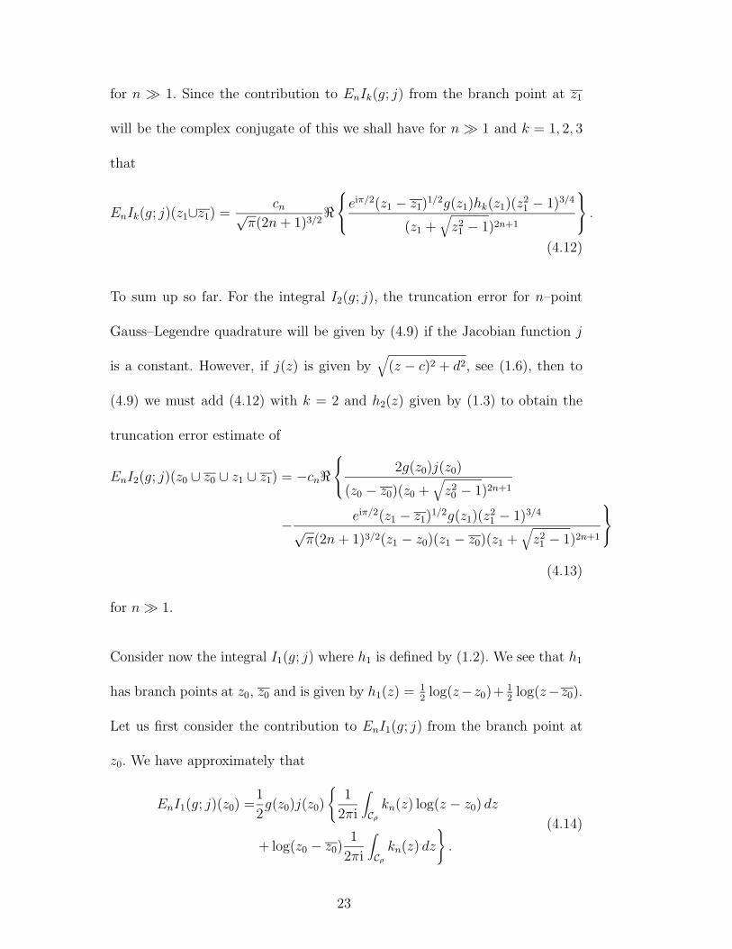
To sum up so far. For the integral I2(g; j), the truncation error for n–point
Gauss–Legendre quadrature will be given by (4.9) if the Jacobian function j
is a constant. However, if j(z) is given by√(z − c)2 + d2, see (1.6), then to
(4.9) we must add (4.12) with k = 2 and h2(z) given by (1.3) to obtain the
truncation error estimate of
EnI2(g; j)(z0 ∪ z0 ∪ z1 ∪ z1) = −cn� 2g(z0)j(z0)
(z0 − z0)(z0 +√z20 − 1)2n+1
− eiπ/2(z1 − z1)1/2g(z1)(z21 − 1)3/4
√π(2n + 1)3/2(z1 − z0)(z1 − z0)(z1 +
√z21 − 1)2n+1
(4.13)
for n� 1.
Consider now the integral I1(g; j) where h1 is defined by (1.2). We see that h1
has branch points at z0, z0 and is given by h1(z) =12log(z−z0)+ 1
2log(z−z0).
Let us first consider the contribution to EnI1(g; j) from the branch point at
z0. We have approximately that
EnI1(g; j)(z0) =1
2g(z0)j(z0)
{1
2πi
∫Cρ
kn(z) log(z − z0) dz
+ log(z0 − z0) 12πi
∫Cρ
kn(z) dz
}.
(4.14)
23

From (A1) and (A3) we may rewrite this as
EnI1(g; j)(z0) =1
2g(z0)j(z0) {Ln(z0; 0) + log(z0 − z0)Kn(0)} . (4.15)
Since Kn(0) = 0 we find from (A3) that for n� 1
EnI1(g; j)(z0) = − cng(z0)j(z0)(z20 − 1)1/2
2(2n+ 1)(z0 +√z20 − 1)2n+1
. (4.16)
Again, since the contribution from the branch point at z0 will be the complex
conjugate of this we have
EnI1(g; j)(z0 ∪ z0) = − cn2n + 1
�g(z0)j(z0)(z
20 − 1)1/2
(z0 +√z20 − 1)2n+1
, (4.17)
for n � 1. If j is a constant then this is the required estimate for EnI1(g; j).
If, however, j is given by (1.6) then to (4.17) we must add the contribution to
the error as given by (4.12) with k = 1, and h1(z) given by (1.2), to give the
overall truncation error estimate
EnI1(g; j)(z0 ∪ z0 ∪ z1 ∪ z1) = − cn2n+ 1
�g(z0)j(z0)(z
20 − 1)1/2
(z0 +√z20 − 1)2n+1
+
eiπ/2(z1 − z1)1/2g(z1) log((z1 − z0)(z1 − z0))(z21 − 1)3/4
2√π(2n+ 1)1/2(z1 +
√z21 − 1)2n+1
(4.18)
for n� 1.
Finally, we must consider the truncation error for the integral I3(g; j) where
h3 is defined in (1.4). Again the function h3 has branch points at z0, z0. In
estimating the truncation error from the branch point at z0 we have, from
24

(1.4), (4.7) and (A2), that approximately
EnI3(g; j)(z0) = (z0 − z0)λg(z0)j(z0)Kn(z0;λ). (4.19)
From (A2) we have that for n� 1
EnI3(g; j)(z0) =cne
−iπλ(z0 − z0)λg(z0)j(z0)(z20 − 1)(λ+1)/2
Γ(−λ)(2n+ 1)λ+1(z0 +√z20 − 1)2n+1
. (4.20)
Again, since EnI3(g; j)(z0) will be the complex conjugate of this we have
EnI3(g; j)(z0∪z0) = 2cnΓ(−λ)(2n + 1)λ+1
�e
−iπλ(z0 − z0)λg(z0)j(z0)(z20 − 1)(λ+1)/2
(z0 +√z20 − 1)2n+1
(4.21)
for n � 1. If j is a constant then this is the required estimate for EnI3(g; j).
If, however, j is given by (1.6) then to (4.21) we must add the contribution
to the error as given by (4.12) with k = 3, and h3(z) given by (1.4), to obtain
the overall truncation error estimate
EnI3(g; j)(z0 ∪ z0 ∪ z1 ∪ z1) = cn2n+ 1
�2e
−iπλ(z0 − z0)λg(z0)j(z0)(z20 − 1)(λ+1)/2
Γ(−λ)(2n + 1)λ(z0 +√z20 − 1)2n+1
+eiπ/2(z1 − z1)1/2g(z1) ((z1 − z0)(z1 − z0))λ (z21 − 1)3/4
√π(2n+ 1)1/2(z1 +
√z21 − 1)2n+1
(4.22)
for n� 1.
Before considering a similar analysis of the truncation errors when n–point
Gauss–Legendre quadrature is applied to the transformed integrals, let us
summarise the results of this section in Table 2.
25
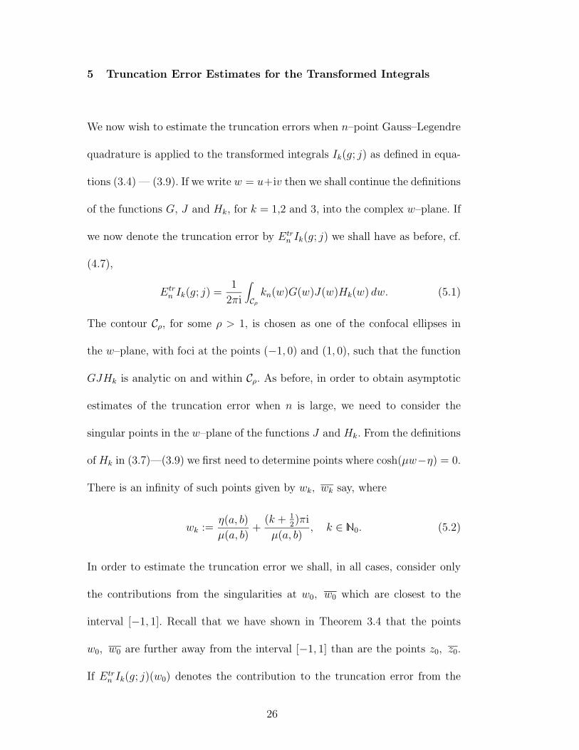
5 Truncation Error Estimates for the Transformed Integrals
We now wish to estimate the truncation errors when n–point Gauss–Legendre
quadrature is applied to the transformed integrals Ik(g; j) as defined in equa-
tions (3.4) — (3.9). If we write w = u+iv then we shall continue the definitions
of the functions G, J and Hk, for k = 1,2 and 3, into the complex w–plane. If
we now denote the truncation error by Etrn Ik(g; j) we shall have as before, cf.
(4.7),
Etrn Ik(g; j) =
1
2πi
∫Cρ
kn(w)G(w)J(w)Hk(w) dw. (5.1)
The contour Cρ, for some ρ > 1, is chosen as one of the confocal ellipses in
the w–plane, with foci at the points (−1, 0) and (1, 0), such that the function
GJHk is analytic on and within Cρ. As before, in order to obtain asymptotic
estimates of the truncation error when n is large, we need to consider the
singular points in the w–plane of the functions J and Hk. From the definitions
ofHk in (3.7)—(3.9) we first need to determine points where cosh(µw−η) = 0.
There is an infinity of such points given by wk, wk say, where
wk :=η(a, b)
µ(a, b)+(k + 1
2)πi
µ(a, b), k ∈ N0. (5.2)
In order to estimate the truncation error we shall, in all cases, consider only
the contributions from the singularities at w0, w0 which are closest to the
interval [−1, 1]. Recall that we have shown in Theorem 3.4 that the points
w0, w0 are further away from the interval [−1, 1] than are the points z0, z0.
If Etrn Ik(g; j)(w0) denotes the contribution to the truncation error from the
26

singularity at w0 then we shall, as a first step, write
Etrn Ik(g; j)(w0) =
G(w0)J(w0)
2πi
∫Cρ
kn(w)Hk(w) dw, (5.3)
approximately. From (3.5), (3.6), the definition of w0 and recalling that z0 =
a+ ib we have
Etrn Ik(g; j)(w0) =
µg(z0)j(z0)
2πi
∫Cρ
kn(w)Hk(w) dw. (5.4)
Let us evaluate this integral in the simplest case, when k = 2. Then H2 has a
simple pole at w0 and we find from (3.8) that its residue is 2/(µ(z0 − z0)). On
letting ρ→ ∞ in (5.4) we find
Etrn I2(g; j)(w0) = −2g(z0)j(z0)kn(w0)
(z0 − z0) . (5.5)
Since Etrn I2(g; j)(w0) will be the complex conjugate of this we find, on using
(4.5), that
Etrn I2(g; j)(w0 ∪ w0) = −4cn�
g(z0)j(z0)
(z0 − z0)(w0 +√w2
0 − 1)2n+1
, (5.6)
for n� 1. If j is a constant then this is the required asymptotic estimate for
EnI2(g; j). On comparing (5.6) with (4.9) we see explicitly for the first time the
advantage of the transformation. In the untransformed case, we see from (4.9)
that the error tends to zero like
O(1/|z0+√z20 − 1|2n+1) whereas from (5.6) the transformed error tends to zero
like
O(1/|w0 +√w2
0 − 1|2n+1). From the discussion in §3 we know that
27

|w0+√w2
0 − 1| > |z0+√z20 − 1| so that the rate of convergence to zero in the
transformed case will be better that in the untransformed case. We shall show
some numerical results for specific examples in §6.
Suppose now that j is given by (1.6) so that from (3.6) we have
J(w) = (a+ b sinh(µw − η)− z1)1/2(a + b sinh(µw − η)− z1)1/2. (5.7)
This function will have branch points where a + b sinh(µw − η) = z1 and
a + b sinh(µw − η) = z1. Again there will be an infinity of such points in the
w–plane. Let w∗1 and w1
∗ be the points closest to [−1, 1] such that
a+ b sinh(µw∗1 − η) = z1; (5.8)
that is
w∗1 =
η
µ+1
µarcsinh
(z1 − ab
). (5.9)
Let us consider Etrn Ik(g; j)(w
∗1) where k may be 1, 2 or 3. From (5.1) we have,
first of all, that this is given approximately by
Etrn Ik(g; j)(w
∗1) =
G(w∗1)Hk(w
∗1)
2πi
∫Cρ
kn(w)J(w) dw. (5.10)
Now, near w∗1, we have from (5.7) that
J(w) = (z1 − z1)1/2 (b(sinh(µw − η)− sinh(µw∗1 − η)))1/2 (5.11)
approximately. On approximating sinh(µw − η) − sinh(µw∗1 − η)) by µ(w −
w∗1) cosh(µw
∗1−η) and observing from (5.8) that b cosh(µw∗
1−η) = ((z1 − z0)(z1 − z0))1/2
28

we find that
J(w) = µ1/2(z1 − z1)1/2 ((z1 − z0)(z1 − z0))1/4 (w − w∗1)
1/2 (5.12)
approximately, in the neighbourhood of w∗1. Since G(w
∗1) = µg(z1) we find
from (5.10), (5.12) and (A2) that
Etrn Ik(g; j)(w
∗1) = µ
3/2g(z1)(z1−z1)1/2 ((z1 − z0)(z1 − z0))1/4Hk(w∗1)Kn(w
∗1;1
2),
(5.13)
for n � 1. From (A2) again we will obtain the required asymptotic estimate
for Etrn Ik(g; j)(w
∗1). Since the contribution to E
trn Ik(g; j) from the singularity
at w1∗ will be the complex conjugate of this we find on addition that
Etrn Ik(g; j)(w
∗1 ∪ w1
∗) =cnµ
3/2
π1/2(2n+ 1)3/2× (5.14)
�e
iπ/2g(z1)(z1 − z1)1/2 ((z1 − z0)(z1 − z0))1/4 (w∗12 − 1)3/4Hk(w
∗1)
(w∗1 +
√w∗
12 − 1)2n+1
for n� 1. We note here that from (3.7)–(3.9) and (5.8) we have
H1(w∗1)=
1
2((z1 − z0)(z1 − z0))1/2 log ((z1 − z0)(z1 − z0)) , (5.15)
H2(w∗1)= ((z1 − z0)(z1 − z0))−1/2 , (5.16)
H3(w∗1)= ((z1 − z0)(z1 − z0))λ+1/2 . (5.17)
29

On recalling (5.6), if j is given by (1.6) then from (5.14) and (5.16)we find
Etrn I2(g; j)(w0 ∪ w0 ∪ w∗
1 ∪ w1∗) =
cn�e
iπ/2µ3/2g(z1)(z1 − z1)1/2 ((z1 − z0)(z1 − z0))−1/4 (w∗12 − 1)3/4
√π(2n+ 1)3/2(w∗
1 +√w∗
12 − 1)2n+1
− 4g(z0)j(z0)
(z0 − z0)(w0 +√w2
0 − 1)2n+1
(5.18)
We must now consider the estimates for Etrn Ik(g; j)(w0 ∪w0) when k = 1 and
3; recall that the estimate for k = 2 has been given in (5.6). From (5.4) we
have
Etrn I1(g; j)(w0) =
µg(z0)j(z0)
2πi
∫Cρ
kn(w)H1(w) dw (5.19)
approximately, where H1(w) is defined by (3.7). We are interested in H1(w)
near w0. Since cosh(µw0 − η) = 0 and sinh(µw0 − η) = eiπ/2 it follows that
near w0
b cosh(µw − η)= b cosh((µw0 − η) + µ(w − w0))
= eiπ/2b sinh(µ(w − w0))
= eiπ/2bµ(w − w0), (5.20)
approximately.
On substituting (5.20) into (3.7) we have that for w close to w0
H1(w) = eiπ/2bµ
[log(bµeiπ/2)(w − w0) + (w − w0) log(w − w0)
]. (5.21)
Substituting this for H1(w) into (5.19) and recalling the definitions of Kn(m)
30

and Ln(z∗;m) from (A1) and (A3) respectively we find
Etrn I1(g; j)(w0) = e
iπ/2bµ2g(z0)j(z0){log(bµeiπ/2)[Kn(1)− w0Kn(0)] + Ln(w0; 1)
}.
(5.22)
For all n ∈ N we know that Kn(0) = Kn(1) = 0 so that from (A3) we find for
n� 1 that
Etrn I1(g; j)(w0) = − cnµ
2
2(2n+ 1)2(z0 − z0)g(z0)j(z0)(w2
0 − 1)(w0 +
√w2
0 − 1)2n+1, (5.23)
on recalling (1.5). Since the contribution from the singularity at w0 will be
the complex conjugate of this we find
Etrn I1(g; j)(w0 ∪ w0) = − cnµ
2
(2n+ 1)2�(z0 − z0)g(z0)j(z0)(w
20 − 1)
(w0 +√w2
0 − 1)2n+1
, (5.24)
for n � 1. When the Jacobian j is a constant this is the estimate for the
truncation error in this case. When j is given by (1.6) we must add to this the
contribution from the singularities at w∗1 and w1
∗ as given by (5.14) together
with (5.15); this gives
Etrn I1(g; j)(w0 ∪ w0 ∪ w∗
1 ∪ w1∗) =
cnµ3/2
(2n+ 1)3/2×
�e
iπ/2g(z1)(z1 − z1)1/2 ((z1 − z0)(z1 − z0))3/4 (w∗12 − 1)3/4 log ((z1 − z0)(z1 − z0))
2√π(w∗
1 +√w∗
12 − 1)2n+1
−√µ(z0 − z0)g(z0)j(z0)(w2
0 − 1)√2n+ 1(w0 +
√w2
0 − 1)2n+1
.
(5.25)
It remains to consider the estimate for Etrn I3(g; j)(w0 ∪ w0). From (3.9) and
31
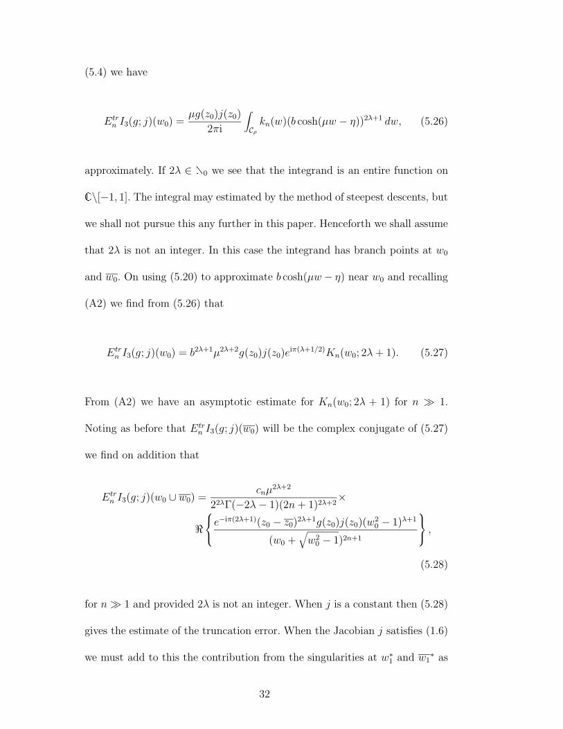
(5.4) we have
Etrn I3(g; j)(w0) =
µg(z0)j(z0)
2πi
∫Cρ
kn(w)(b cosh(µw − η))2λ+1 dw, (5.26)
approximately. If 2λ ∈ N0 we see that the integrand is an entire function on
C\[−1, 1]. The integral may estimated by the method of steepest descents, but
we shall not pursue this any further in this paper. Henceforth we shall assume
that 2λ is not an integer. In this case the integrand has branch points at w0
and w0. On using (5.20) to approximate b cosh(µw− η) near w0 and recalling
(A2) we find from (5.26) that
Etrn I3(g; j)(w0) = b
2λ+1µ2λ+2g(z0)j(z0)eiπ(λ+1/2)Kn(w0; 2λ+ 1). (5.27)
From (A2) we have an asymptotic estimate for Kn(w0; 2λ + 1) for n � 1.
Noting as before that Etrn I3(g; j)(w0) will be the complex conjugate of (5.27)
we find on addition that
Etrn I3(g; j)(w0 ∪ w0) =
cnµ2λ+2
22λΓ(−2λ− 1)(2n+ 1)2λ+2×
�e
−iπ(2λ+1)(z0 − z0)2λ+1g(z0)j(z0)(w20 − 1)λ+1
(w0 +√w2
0 − 1)2n+1
,
(5.28)
for n� 1 and provided 2λ is not an integer. When j is a constant then (5.28)
gives the estimate of the truncation error. When the Jacobian j satisfies (1.6)
we must add to this the contribution from the singularities at w∗1 and w1
∗ as
32

given in (5.14) where H3(w∗1) is given by (5.17). We find
Etrn I3(g; j)(w0 ∪ w0 ∪ w∗
1 ∪ w1∗) =
cnµ3/2
(2n+ 1)3/2�e
iπ/2g(z1)(z1 − z1)1/2 ((z1 − z0)(z1 − z0))λ+3/4 (w∗12 − 1)3/4
√π(w∗
1 +√w∗
12 − 1)2n+1
+µ2λ+1/2e−iπ(2λ+1)(z0 − z0)2λ+1g(z0)j(z0)(w
20 − 1)λ+1
22λΓ(−2λ− 1)(2n+ 1)2λ+1/2(w0 +√w2
0 − 1)2n+1
.
(5.29)
We have summarised these results for the transformed integrals in Table 3.
6 Some Numerical Examples
Having obtained asymptotic estimates of the truncation errors in the quadra-
ture formulae, let us now see how good they are. In Johnston and Elliott [15], it
has been demonstrated at length how effective the transformation (1.7) can be.
Here we shall consider just four examples which, in addition to demonstrating
again the effectiveness of the transformation, also compares the asymptotic
estimates with the actual truncation errors. Although these estimates can be
excellent we shall also see that there may be limitations.
Example 1
Consider the integral I1 where
I1 :=1
2
∫ 1
−1
x
2(x− 1) log((x− a)2 + b2) dx. (6.1)
33
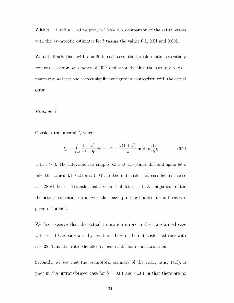
With a = 12and n = 20 we give, in Table 4, a comparison of the actual errors
with the asymptotic estimates for b taking the values 0.1, 0.01 and 0.001.
We note firstly that, with n = 20 in each case, the transformation essentially
reduces the error by a factor of 10−6 and secondly, that the asymptotic esti-
mates give at least one correct significant figure in comparison with the actual
error.
Example 2
Consider the integral I2 where
I2 :=∫ 1
−1
1− x2
x2 + b2dx = −2 + 2(1 + b2)
barctan(
1
b), (6.2)
with b > 0. The integrand has simple poles at the points ±ib and again let b
take the values 0.1, 0.01 and 0.001. In the untransformed case let us choose
n = 28 while in the transformed case we shall let n = 10. A comparison of the
the actual truncation errors with their asymptotic estimates for both cases is
given in Table 5.
We first observe that the actual truncation errors in the transformed case
with n = 10 are substantially less than those in the untransformed case with
n = 28. This illustrates the effectiveness of the sinh transformation.
Secondly, we see that the asymptotic estimate of the error, using (4.9), is
poor in the untransformed case for b = 0.01 and 0.001 in that there are no
34

correct significant digits. This suggests that the asymptotic estimate for kn,
as given by (4.5) and (4.6), is not good enough for such small values of b. In
Elliott [18], alternative asymptotic estimates for kn are given which will be
more appropriate in this case. From equations (2.13) and (2.14) of [18] we find
on taking the first terms only in these expansions that an alternative estimate
for kn when n� 1 is given by
kn(z) =2K0((n+ 1/2) arccosh z)
I0((n+ 1/2) arccosh z). (6.3)
With this estimate for kn we find (cf. (4.9))
EnI2 =2(1 + b2)
b�{iK0((n+ 1/2) arccosh(ib))
I0((n+ 1/2) arccosh(ib))
}. (6.4)
In Table 6 we compare this asymptotic estimate with the actual errors when
n = 28 and b = 0.1, 0.01 and 0.001. We see that the new asymptotic estimates
are better than those given in Table 5 when b = 0.01 and 0.001. However,
this comes at a cost of using modified Bessel functions rather than elementary
functions.
Example 3
Consider the integral I3 where
I3 :=∫ 1
−1
x
2(x+ 1)((x− a)2 + b2)−0.4 dx. (6.5)
35

In this example we shall choose a = 0.25 and again let b take the values 0.1,
0.01, 0.001. The actual and asymptotic errors in the untransformed integral
with n = 25 and in the transformed integral with n = 15, are displayed in
Table 7.
Again, it is interesting to note that 15 point Gauss–Legendre quadrature ap-
plied to the transformed integral gives considerably smaller truncation er-
rors than 25 point Gauss-Legendre quadrature in the untransformed case.
Although most of the asymptotic estimates are good it should be noted that
in the untransformed case when b = 0.001 the asymptotic estimate is about
twice that of the actual error.
Example 4
In the final example we shall consider an integral where the Jacobian function j
is not constant on the interval of integration. The Jacobian we have introduced
arises when a curved quadratic boundary element is interpolated between the
points (1, 1), (2, 12) and (3, 1). Consider the integral
I4 :=∫ 1
−1
√1 + x2
(x− a)2 + b2 dx. (6.6)
On writing z0 = a+ib it may be shown, on splitting the integrand into partial
fractions, that
I4 = 2 arcsinh 1− 1
b�√z20 + 1 log
√2z0 +
√z20 + 1√
2z0 −√z20 + 1
. (6.7)
36

In this example we shall choose a = 0.75 and let b take the values 0.1, 0.01
and 0.001. For the untransformed integral we shall choose n = 30 and, for the
transformed integral, n = 15. The results are given in Table 8.
From Table 8 we note that 15 point Gauss-Legendre quadrature on the trans-
formed integral gives a truncation error which is two or three orders of mag-
nitude smaller than that for 30 point Gauss-Legendre quadrature on the un-
transformed integral. Although the asymptotic estimates compare well with
the actual truncation errors in the transformed case, they are not as good in
the untransformed case even though the value of n has doubled. In Table 9 we
give the ratios of the actual to the asymptotic estimates arising from Table 8.
Since, as we have shown in §3, the transformation takes the singularities fur-
ther away from the interval of integration [−1, 1], it is perhaps not surprising
that in the transformed case the estimates are within about 1% of the actual
errors.
In conclusion, we have illustrated by considering four example how, in many
cases, the asymptotic estimate of the truncation error in the quadrature rule
gives a good approximation to the actual error. However, it should be noted
that the asymptotic estimates may not be good when the singularities of
the integrand are very close to the interval of integration and n is not taken
large enough. In all cases we have illustrated that the truncation error is
reduced, at times dramatically, when Gauss-Legendre quadrature is applied
37

to the transformed integral.
Appendix: Evaluation of Three Contour Integrals
It is convenient to consider here the evaluation of three contour integrals which
arise in the analysis of §§4 and 5. Firstly, we will show that the function
Kn(m) :=1
2πi
∫Cρ
kn(z)zm dz = 0, (A1)
where m ∈ N0 with m ≤ 2n− 1 and the contour Cρ is any ellipse with ρ > 1.
We will also show that
Kn(z∗;λ) :=1
2πi
∫Cρ
kn(z)(z−z∗)λ dz = cne−iπλ(z2∗ − 1)(λ+1)/2
Γ(−λ)(2n+ 1)λ+1(z∗ +√z2∗ − 1)2n+1
,
(A2)
and that
Ln(z∗;m) :=1
2πi
∫Cρ
kn(z)(z − z∗)m log(z − z∗) dz
=− cnm!(z2∗ − 1)(m+1)/2
(2n+ 1)m+1(z∗ +√z2∗ − 1)2n+1
,
(A3)
for n� 1. In these equations z∗ is a point in the upper–half plane such that
z∗ = r∗eiα where r∗ > 0 and 0 < α < π; λ in (A2) is not an integer and is
such that −1 < λ < 2n − 1. Finally, in (A3), m ∈ N0 with 0 ≤ m ≤ 2n − 1.
In both cases Cρ is an ellipse with ρ chosen so that the point z∗ is outside Cρ.
To begin, recall from (4.1) and (4.2) that Kn(m) is simply the truncation error
arising when n–point Gauss–Legendre quadrature is applied to the function
xm. It is well known, since we are assuming m ≤ 2n−1, that the error is zero.
38

We can also show this by observing first of all from (4.5), that if z ∈ Cρ for any
ρ > 1 then |kn(z)| ≤ cn/ρ2n+1, when n � 1. Since the length of the contour
Cρ is less that π(ρ + 1/ρ), the circumference of the circle with centre at the
origin and radius the semi–major axis of Cρ, and since |z| ≤ |z+√z2 − 1| = ρ
for z ∈ Cρ it follows from (A1) that
|Kn(m)| ≤ c/ρ2n−m (A4)
for some c independent of ρ. On letting ρ→ ∞ and recalling that kn(z)zm is
analytic for z ∈ C\[−1, 1], we have that |Kn(m)| = 0 since we have assumed
m ≤ 2n− 1. Thus Kn(m) = 0.
In order to evaluate Kn and Ln we shall cut the z–plane from z∗ = r∗eiα to
∞eiα and then let ρ → ∞. In order that the contour is deformed only over
regions in the z–plane where the integrand is analytic, the contour Cρ becomes
AB ∪CD ∪ C′ρ′ , see Figure 1. Along AB we have z = z∗ + reiα with r from∞
to 0; along CD, z = z∗+ rei(α−2π) with r from 0 to∞. The contour C′ρ′ is that
part of the ellipse Cρ′ from D to A, where ρ′ is “large”. From the conditions
put on λ and m above we see that the integrals around C′ρ′ will tend to zero
in both cases as ρ′ → ∞. Thus we may rewrite Kn(z∗;λ) and Ln(z∗;m) as
Kn(z∗;λ) = −1πe−iπλ sin(πλ)Jn(z∗;λ) (A5)
and
Ln(z∗;m) = −Jn(z∗;m) (A6)
39

respectively, where Jn(z∗;µ) for −1 ≤ µ ≤ 2n− 1 is defined by
Jn(z∗;µ) := limR→∞
∫ R
0kn((r∗ + r)eiα)(reiα)µeiα dr, (A7)
where µ may be an integer. We shall estimate Jn(z∗;µ) for large n by using
the asymptotic form of kn as given by (4.5) and (4.6). We find
Jn(z∗;µ) = cn limR→∞
∫ R
0
(reiα)µeiα dr
((r∗ + r)eiα +√((r∗ + r)eiα)2 − 1)2n+1
. (A8)
To evaluate this integral, let us first write
(r∗ + r)eiα = cosh θ, r∗eiα = cosh θ∗, eiα dr = sinh θ dθ. (A9)
On recalling, see Abramowitz and Stegun [17, §4.6.32], that for R � 1,
arccosh(Reiα) = log(2R) + iα +O(1/R2) we find from (A8) and (A9) that
Jn(z∗;µ) = cn limR→∞
∫ log(2R)+iα
θ∗e−(2n+1)θ sinh θ(cosh θ − cosh θ∗)µ dθ. (A10)
For n� 1, the major contribution to this integral will come from the neigh-
bourhood of θ∗. On replacing sinh θ by sinh θ∗ and cosh θ − cosh θ∗ by (θ −
θ∗) sinh θ∗ we find
Jn(z∗;µ) = cn(sinh θ∗)µ+1e−(2n+1)θ∗ limR→∞
∫ log(2R)+iα
θ∗e−(2n+1)(θ−θ∗)(θ − θ∗)µ dθ.
(A11)
Now from (A9) we have z∗ = cosh θ∗ so that sinh θ∗ =√z2∗ − 1 and e−θ∗ =
1/(z∗ +√z2∗ − 1). On writing θ − θ∗ = φ, dθ = dφ we have
40

limR→∞
∫ log(2R)+iα
θ∗e−(2n+1)(θ−θ∗)(θ − θ∗)µ dθ
= limR→∞
∫ log(2R)+iα−arccosh(z∗)
0e−(2n+1)φφµ dφ
=∫ ∞
0e−(2n+1)φφµ dφ, by Cauchy′s theorem,
=Γ(µ+ 1)/(2n+ 1)µ+1, (A12)
since µ > −1; see, for example, Erdelyi [19, §4.3(1)]. From (A11) and (A12)
we have for n� 1
Jn(z∗;µ) =cnΓ(µ+ 1)(z
2∗ − 1)(µ+1)/2
(2n+ 1)µ+1(z∗ +√z2∗ − 1)2n+1
. (A13)
We can now give the required asymptotic estimates for the integrals. From
(A5) and (A13) and the reflection formula for the gamma function [17, §6.1.17]
we obtain (A2) and from (A6) and (A13) we get (A3).
References
[1] J. D. Donaldson, D. Elliott, A unified approach to quadrature rules with
asymptotic estimates of their remainders, SIAM Journal of Numerical Analysis
9 (1972) 573–602.
[2] C. A. Brebbia, J. Dominguez, Boundary Elements An Introductory Course, 2nd
Edition, Computational Mechanics Publications, Southampton, 1992.
[3] J. C. F. Telles, A self–adaptive co–ordinate transformation for efficient
numerical evaluation of general boundary element integrals, International
Journal for Numerical Methods in Engineering 24 (1987) 959–973.
41
[4] J. Sanz-Serna, M. Doblare, E. Alarcon, Remarks on methods for the
computation of boundary-element integrals by co-ordinate transformation,
Communications in Numerical Methods in Engineering. 6 (1990) 121–123.
[5] J. C. F. Telles, R. F. Oliveira, Third degree polynomial transformation for
boundary element integrals: Further improvements, Engineering Analysis with
Boundary Elements 13 (1994) 135–141.
[6] P. R. Johnston, D. Elliott, A generalisation of Telles’ method for evaluating
weakly singular boundary element integrals, Journal of Computational and
Applied Mathematics 131 (1–2) (2001) 223–241.
[7] B. I. Yun, P. Kim, A new sigmoidal transformation for weakly singular integrals
in the boundary element method, SIAM Journal for Scientific Computing 24 (4)
(2003) 1203–1217.
[8] B. I. Yun, A composite transformation for numerical integration of singular
integrals in the bem, International Journal for Numerical Methods in
Engineering 57 (13) (2003) 1883–1898.
[9] B. I. Yun, An extended sigmoidal transformation technique for evaluating
weakly singular integrals without splitting the integration interval, SIAM
Journal for Scientific Computing 25 (1) (2003) 284–301.
[10] B. I. Yun, A non-linear co-ordinate transformation for accurate numerical
evaluation of weakly singular integrals, Communications in Numerical Methods
in Engineering 20 (2003) 401–417.
[11] P. R. Johnston, Application of sigmoidal transformations to weakly singular and
42

near-singular boundary element integrals, International Journal for Numerical
Methods in Engineering 45 (10) (1999) 1333–1348.
[12] P. R. Johnston, Semi–sigmoidal transformations for evaluating weakly singular
boundary element integrals, International Journal for Numerical Methods in
Engineering 47 (10) (2000) 1709–1730.
[13] P. R. Johnston, D. Elliott, Error estimation of quadrature rules for evaluating
singular integrals in boundary element problems, International Journal for
Numerical Methods in Engineering. 48 (7) (2000) 949–962.
[14] P. R. Johnston, D. Elliott, Transformations for evaluating singular boundary
element integrals, Journal of Computational and Applied Mathematics 146 (2)
(2002) 231–251.
[15] P. R. Johnston, D. Elliott, A sinh transformation for evaluating nearly singular
boundary element integrals, International Journal for Numerical Methods in
Engineering 62 (4) (2005) 564–578.
[16] J. W. Kitchen, Calculus of One Variable, Addison–Wesley, Reading, Mass.,
1968.
[17] M. Abramowitz, I. A. Stegun, Handbook of Mathematical Functions, Dover,
New York, 1972.
[18] D. Elliott, Uniform asymptotic expansions of the Jacobi polynomials and an
associated function, Mathematics of Computation 25 (1971) 309–315.
[19] A. Erdelyi (Ed.), Tables of Integral Transforms, Vol. 1, McGraw–Hill, New
York, 1954.
43

Captions
Table 1: Values of ρ(0, t(0, b))/ρ(0, b).
Table 2: Truncation error EnIk(g; j) for n� 1.
Table 3: Truncation error Etrn Ik(g; j) for n� 1.
Table 4: Actual errors and asymptotic estimates for errors in the evaluation
of the integral I1 for various values of b. For both the untransformed and
transformed integrals with n = 20.
Table 5: Actual errors and asymptotic estimates for errors in the evaluation
of the integral I2 for various values of b. For the untransformed integral with
n = 28 and for the transformed integral with n = 10.
Table 6: Actual errors and asymptotic estimates for errors in the evaluation
of the integral I2 for various values of b for the untransformed integral with
n = 28.
Table 7: Actual errors and asymptotic estimates for errors in the evaluation
of the integral I3 for various values of b. For the untransformed integral with
n = 25 and for the transformed integral with n = 15.
Table 8: Actual errors and asymptotic estimates for errors in the evaluation
of the integral I4 for various values of b. For the untransformed integral with
n = 30 and for the transformed integral with n = 15.
44

Table 9: Ratio of the actual and asymptotic error estimates for evaluation
of the integral I4. For the untransformed integral with n = 30 and for the
transformed integral with n = 15.
Figure 1: z–plane
45

b ρ(0, t(0, b))/ρ(0, b)
1 1.5847
0.1 1.4958
0.01 1.3262
0.001 1.2266
0.0001 1.1710
Table 1
k = 1 k = 2 k = 3
j a constant (4.17) (4.9) (4.21)
j given by (1.6) (4.18) (4.13) (4.22)
Table 2
k = 1 k = 2 k = 3
j a constant (5.24) (5.6) (5.28)
j given by (1.6) (5.25) (5.18) (5.29)
Table 3
46

Untransformed integral, n = 20 Transformed integral, n = 20
b Actual Error Asymp. Est. (4.17) Actual Error Asymp. Est. (5.24)
0.1 −1.6678 × 10⁻⁴ −1.1371 × 10⁻⁴ −6.4210 × 10⁻¹³ −6.1832 × 10⁻¹³
0.01 −9.7186 × 10⁻³ −8.8025 × 10⁻³ +1.2757 × 10⁻⁹ +1.2498 × 10⁻⁹
0.001 −1.1320 × 10⁻² −1.3531 × 10⁻² +1.9104 × 10⁻⁸ +1.9278 × 10⁻⁸
Table 4
Untransformed integral, n = 28 Transformed integral, n = 10
b Actual Error Asymp. Est. (4.9) Actual Error Asymp. Est. (5.6)
0.1 2.55 × 10⁻¹ 2.12 × 10⁻¹ +3.2802 × 10⁻³ +3.2386 × 10⁻³
0.01 1.574 × 10² 3.523 × 10² +2.6894 × 100 +2.6496 × 100
0.001 3.132 × 10³ 5.883 × 10³ 1.6581 × 10² +1.6492 × 10²
Table 5
47

Untransformed integral, n = 28
b Actual Error Asymp. Est. (6.4)
0.1 2.55 × 10⁻¹ 2.14 × 10⁻¹
0.01 1.574 × 10² 2.270 × 10²
0.001 3.132 × 10³ 3.052 × 10³
Table 6
Untransformed integral, n = 25 Transformed integral, n = 15
b Actual Error Asymp. Est. (4.21) Actual Error Asymp. Est. (5.28)
0.1 −6.5044 × 10⁻⁴ −6.7175 × 10⁻⁴ −2.1043 × 10⁻⁹ −2.0584 × 10⁻⁹
0.01 −2.6430 × 10⁻¹ −2.1443 × 10⁻¹ +1.8532 × 10⁻⁷ +1.7603 × 10⁻⁷
0.001 −4.8955 × 10⁻¹ −8.7740 × 10⁻¹ +1.4016 × 10⁻⁵ +1.3770 × 10⁻⁵
Table 7
48

Untransformed integral, n = 30 Transformed integral, n = 15
b Actual Error Asymp. Est. (4.13) Actual Error Asymp. Est. (5.18)
0.1 +6.5008 × 10⁻³ +6.5187 × 10⁻³ +1.2636 × 10⁻⁶ +1.2501 × 10⁻⁶
0.01 +1.2485 × 10² +3.3268 × 101 −6.7516 × 10⁻² −6.6706 × 10⁻²
0.001 +3.5953 × 10³ +7.3809 × 10² +1.0042 × 101 +9.9387 × 100
Table 8
49

Untransformed integral, n = 30 Transformed integral, n = 15
b Actual/Asymptotic Actual/Asymptotic
0.1 0.9970 1.0108
0.01 3.7530 1.0121
0.001 4.8710 1.0104
Table 9
50

b b
b
α-10
1
C′ρ′
x
y
A
B
C
D
z∗
r∗
Fig. 1.
51

Replies to Reviewer’s Comments:CAM-D-05-00443
Title: Error Analysis for a sinh Transformation used inEvaluating Nearly Singular Boundary Element Integrals
Authors: David Elliott and Peter R. Johnston
Reviewer 1
1. We have added further explanation on page 17 (of the new version ofthe manuscript) to help explain the concept of “ρ → ∞”.
2. We have reworked Example 2 on pp 27–28 and hope that this is carriedout to the satisfaction of the reviewer.
3. We have split equation (2.12) over three lines.
4. The large gaps in the type setting on page 23 are due to the style filesupplied by the publisher. This should be addressed by the professionaltypesetters when and if the manuscript is published.
Reviewer 2
1. We cannot help the error analysis looking excessive. We have tried tokeep it as short as possible.
2. We have made a comment on ρ1/ρ after Theorem 3.4. Unfortunatelywe cannot prove it, but it is useful to leave as a conjecture.
3. Computing Galerkin double integrals is outside the brief for this paper.
4. Surely the inclusion of the function j in equation (1.1) is what you getwith curved boundaries. Please see Example 4 on pp 29–30.
5. Davis and Rabinowitz in chapter 4 of their book give either upperbounds on errors or the Donaldson/Elliott asymptotic analysis for Gauss–Legendre quadrature. Upper bounds are not as good for comparing er-rors as are asymptotic estimates. But of course the latter require morework.
1
Replies to Reviewers' Comments

6. The assumption around the old equation (4.8) was a bit too sweepingand not correct in all cases. We have modified the paragraph and in sodoing removed the old equation (4.8).
7. The reviewer seems to have missed the point. For “close” singularitiesa quadrature rule with a low number of nodes does not give a goodresult. We have demonstrated this. The last two sentences do notmake much sense to us and therefore we cannot respond.
Major Changes
Please note that in the revised manuscript we have made two major changes:
1. We have given a simpler proof of Theorem 3.4
2. Example 2 and the corresponding Tables have been completely re-worked.
2
Top Related