


Languages
Pages
Legal


S1
Magnetic Levitation to Characterize the Kinetics of Free-Radical
Polymerization
Supporting Information
Shencheng Ge1, Sergey N. Semenov1, Amit A. Nagarkar1, Jonathan Milette1, Dionysios
C. Christodouleas1, Li Yuan1, and George M. Whitesides1,2,3*
1 Department of Chemistry & Chemical Biology, Harvard University, 12 Oxford Street,
Cambridge, MA 02138, USA
2 Wyss Institute for Biologically Inspired Engineering, Harvard University, 60 Oxford
Street, Cambridge, MA 02138, USA
3 Kavli Institute for Bionano Science & Technology, Harvard University, 29 Oxford
Street Cambridge, MA 02138, USA
*Corresponding author: [email protected]

S2
Table of contents
Experimental procedures
Calibration of the MagLev device (S4)
Treatment of data (S4)
Preparation of monomers, initiators, solvents, and paramagnetic medium (S4)
Polymerization of PDMS prepolymers (S5)
Thermal polymerization including bulk and suspension polymerization (S6)
Photopolymerization (S7)
Measurement of fractional conversion of the monomer using 1H NMR (S7)
Measurement of temperature of a polymerizing drop (S8)
Polymerization in the presence of solid materials (S9)
Design of the device and alternative approaches (S9)
Correlation of the concentration and the fractional conversion of monomer (S12)
Theoretical model to describe the rate of polymerization of a spherical drop (S12)
Tables
Table S1 Organic liquids as density standards (S18)
Table S2 Calculating the density of a polymerizing sample (S19)
Figures
Figure S1 A MagLev device used in this study (S20)
Figure S2 Plots of calibration using organic solvents and monomers (S21)
Figure S3 MagLev to monitor suspension polymerization (S22)

S3
Figure S4 Spectra of absorption (S23)
Figure S5 Theoretical model to derive the rate of polymerization of a drop (S24)
Figure S6 Correction term and the average rate of polymerization of a drop (S25)
Figure S7 Comparison of MagLev and 1H NMR (S26)
Figure S8 Overlaid 1H NMR spectra (S27, individual spectrum appended)
Figure S9 Change in shape of polymerizing drops (S33)
Figure S10 Measurement of temperature of a polymerizing drop (S34)
Figure S11 Gel effect of polymerizing drops having different volumes (S35)

S4
Experimental procedures
Calibration of the MagLev device
We used small drops (1-5 L, ~1.2 - ~2.1 mm in diameter) of hydrophobic
organic solvents and liquids of low-molecular-weight monomers with known densities to
establish the calibration plots. Table S1 shows a list of suitable hydrophobic organic
liquids for the purpose of calibration. Large standard glass beads (~ 4 mm in diameter)
with precisely calibrated densities that we commonly used to establish the calibration
plots are not preferred owing to their relatively large sizes and often non-spherical
shapes, and thus a greater experimental uncertainties in determining the centroids of the
beads.1
Treatment of data
We used imageJ to analyze the images and manually determined the heights of
the sample drops. Briefly, we drew a line across the centroid of the drop on the image and
in parallel to the edge of the magnets, and read the height of the drop using the scale on
the ruler (where the line intersects the scale) with a precision of ±0.1 mm (one tenth of
the smallest division on the ruler). We did not read h to a higher precision (the ultimate
limit in this experiment is the size of a single pixel on the image, ±0.025 mm) because the
precision of the density values reported by the vendors is limited to ±~0.001, which
translates to an estimated uncertainty in h of ±0.1 mm (using an aqueous solution of 0.5
M MnCl2).
Preparation of monomers, initiators, solvents, and paramagnetic medium

S5
In general, inhibitors including 4-Methoxyphenol and O2 dissolved in the liquids
of monomers were removed by running the liquids of monomers through an Al2O3
column, and subsequently, performing freeze-and-thaw cycles (at least 3x). The purified
monomer was stored at -4 oC under Ar until use. Dissolved O2 in solvents and aqueous
paramagnetic solutions were removed by purging the solvents or aqueous solutions by Ar
for at least 30 min. All solvents and solutions were stored in a gloved box with a
regulated gas environment (N2 atmosphere, O2 <0.5%, v/v%) at room temperature. In
cases where the conversions of monomers at the endpoint (not kinetics) were concerned,
the liquids of monomers were used as received without removing the inhibitors because
the inhibitors would be consumed completely before polymerization initiates, and
therefore, would not affect the net conversions of monomers.
Thermal initiators (benzoyl peroxide, sigma #179981, and azobisisobutyronitrile,
sigma #441090) and photo-initiator (2,2-dimethoxy-2-phenylacetophenone, sigma
#196118) were used as received.
Procedures for polymerization of PDMS prepolymers
PDMS base and catalyst (Dow Corning, Sylgard® 184) were mixed at a weight
ratio of 10:1, and degassed using vacuum. A plastic pipette was used to transfer a small
quantity of the mixture, and held above the cuvette containing an aqueous solution of
MnCl2, until a small drop (~10 L) of the mixture dripped from the pipette tip. Once the
drop entered the solution (before it floated and became trapped at the interface between
the air and the aqueous medium), the cuvette was inserted immediately into the gap
between the two magnets. The levitation height was measured and recorded. The

S6
remaining mixture of the PDMS prepolymer and catalyst was allowed to crosslink at
room temperature for 24 h. A small piece was cut from the crosslinked PDMS slab and
placed into the same MnCl2 solution for measurement of density.
Procedures for thermal polymerization including bulk and suspension
polymerization
Bulk polymerization was performed in small, sealed glass vials (~2 mL). A
mixture including a liquid of a monomer and a thermal initiator was prepared in a glove
box (N2 atmosphere, O2 <0.5%, v/v%), and small aliquots (200 L) were sealed into
small glass vials. The sealed glass vials were removed from the glove box and transferred
to a chemical hood in which the samples were heated using a temperature-regulated oil
bath. At the end of a specified time, the vials were immediately placed on ice to stop the
reaction, and a small aliquot (~1 – 10 L) of the reaction mixture was transferred using a
laboratory pipettor to a MagLev device for density measurement. The sample drop
reached equilibrium in ~1 s or less in the MagLev device used for density measurement.
Suspension polymerization was performed in either sealed glass vials or an open
glass flask (50 – 200 mL, to facilitate continuous sampling and kinetic monitoring). To
simplify the procedure, we used the same aqueous MnCl2 solution both to suspend the
reaction mixture in the glass flask, and to measure the densities of the reacting mixtures
using MagLev. Aliquots of the reacting mixture (~0.5-1 mL) were periodically removed
using a pipettor and a large-bore tip (we simply cut 1-mL pipette tips to enlarge the size
the opening, and thus, to minimize clogging of drops at the pipette tips), cooled by a bath

S7
of the same MnCl2 solution used to suspend the reaction mixture, and measured in a
MagLev device.
Procedures for photopolymerization
Photopolymerization was performed directly in a MagLev device by levitating a
drop of reaction mixture containing a monomer and a photoinitiator in an aqueous MnCl2
solution, and irradiating it with a UV lamp (365 nm, Blak ray, model UVL-21).
Briefly, a reaction mixture of a monomer, a photoinitiator, and a solvent (if used)
was prepared in a glove box (N2 atmosphere, O2 <0.5%, v/v%), and a small aliquot (~1 -
~50 L) was levitated in an aqueous solution of MnCl2 (usually pre-saturated with the
monomer). The cuvette (a standard, disposable UV-grade cuvette cut to 25 mm in height
to fit the MagLev device, sigma #z188018) was then sealed using a double-side tape
(Adhesive Research, #ARSEAL®90880) by pushing the cuvette firmly against the top
magnet. The MagLev device along with the cuvette and the levitated drop of monomer
liquid was transferred, with care not to allow the drop to stick to the cuvette, from the
glove box to a chemical hood. A UV lamp (365 nm, Blak ray, model UVL-21) was
positioned at a distance of 9 cm from the central axis of the MagLev device and used to
initiate the photopolymerization. The airflow in the chemical hood helped stabilize the
temperature of the paramagnetic medium and the polymerizing drop while they were
continuously irradiated with a UV light.
Measurement of fractional conversion of the monomer using 1H NMR

S8
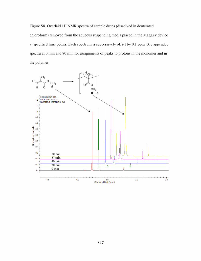
For this experiment of validation, we performed photopolymerization of methyl
methacrylate in the open air (without removing inhibitors such as oxygen) initiated by
2,2-dimethoxy-2-phenylacetophenone (5%, wt%) and UV irradiation at 365 nm (UVGL-
25, UVP LLC, Upland, CA) in the MagLev device. We repeated the same experiments
four times, and removed the sample drops from the MagLev device using a glass pipet at
the specified time points during the time course of photopolymerization (20, 40, 57, 80
min). We then dissolved the sample in deuterated chloroform (~0.5 mL), and recorded
the 1H NMR spectra on a 600 MHz NMR spectrometer. The characteristic shifts of
protons in the methyl ester in methyl methacrylate appear at 3.76 ppm, which are well
separated from the chemical shifts of the same protons in the polymer at 3.60 ppm. We
integrated the areas of these peaks, and estimated the fractional conversion of methyl
methacrylate during polymerization.
Measurement of temperature of a polymerizing drop
We inserted a small (diameter of the wire: 125 m) thermocouple (#CHAL-005,
Omega Engineering, CT) in the MagLev device to measure the temperature of a
polymerizing drop. The thermocouple has a specified response time of <0.1 sec in still
water, and the digital thermometer (#HH11C, Omega Engineering, CT) has a specified
precision of 0.1 oC. We placed a small drop containing methyl methacrylate and
photoinitiator, 2,2-dimethoxy-2-phenylacetophenone (5%, wt%) on the tip of the
thermocouple, and also added a second drop that levitated in the MagLev device without
physical contact. We initiated photopolymerization using 365 nm UV irradiation, and

S9
measured the levitation heights of the nonadherent drop, and the temperature of the
adherent drop over time.
Procedures for polymerization in the presence of solid materials
We performed all polymerizations in the presence of solid materials in a chemical
hood at ambient conditions, and used the chemicals as received (without further
purifications). The solid materials included the following three types in the form of thin,
non-woven veils: aramid (Aramid tissue, ACP composites, Livermore, CA), carbon fiber
(carbon-fiber tissue, ACP composites, Livermore, CA), and glass fiber (fiberglass tissue,
ACP composites, Livermore, CA). We used 3-mm biopsy punches to make discs of these
materials to facilitate the determination of the centers, and thus, the levitation heights, of
the samples during polymerization.
For a typical experiment, we first dissolved benzoyl peroxide (5%, wt%) in a
liquid of monomer methyl methacrylate, added 4,N,N-trimethylaniline (5 L) to a small
aliquot (95 L) of the mixture, immediately mixed it on a vortex (and recorded the
starting time of the polymerization), dipped a disc of a solid material in the reacting
mixture, and quickly transferred the disc to a MagLev device for density measurements.
Design of the device and alternative approaches
In this work, we assembled a MagLev device (Figure S1), rather than using the
approaches (i)-(iii) discussed below, to perform polymerizations for one practical reason:
to retain the operational simplicity of the standard configuration of MagLev to perform
density measurements—we simply add a drop of the monomer, and then monitor
polymerization (upon initiation), without requiring additional manipulations.

S10
The standard configuration of MagLev cannot directly levitate hydrophobic
organic liquids (including liquids of monomers, e.g. methyl methacrylate) having
densities less than water. This shortcoming arises because of its relatively narrow range
of accessible densities spanning from 1 to ~3 g/cm3 using aqueous solutions of simple
paramagnetic salts (e.g. MnCl2 and GdCl3).1
Three approaches we could (potentially) exploit based on the standard
configuration or its variants include: (i) Tilted MagLev.2 This variant of MagLev can
measure the entire range of densities observed in matter at ambient conditions (from ~ 0
g/cm3 to ~23 g/cm3); it, however, requires tilting the standard MagLev device with
respect to the vector of gravity, and rotating the sample container to minimize the impact
of friction on density measurements (the sample, in this configuration of MagLev, is in
physical contact with the sample container). The additional manipulations add
operational complexity to the experimental protocol of density measurements. (ii) The
use of dense solvents (or inert solids) to prepare the sample. We mix a light liquid with a
dense liquid (or an inert solid, such as a glass bead with known volume, density, and
mass) to tune the density of the mixture so that it falls in the accessible range of densities
of the standard configuration of MagLev. While this approach offers a simple option to
levitate light organic liquids, it uses additional components (i.e. solvents or solids) and
also dilutes the change in density associated with the target liquid during, for example,
polymerization. (iii) The use of light suspending medium. We prepare a light suspending
medium using alcohols and other polar organic solvents (e.g. N,N-dimethylformamide or
dimethylsulfoxide). While this approach works for solid samples of polymers,3 it may be

S11
sub-optimal to study polymerization because of the compatibility of the solubilities of the
participating components in polymerization with the suspending medium.
Given the shortcomings of these three approaches, we, therefore, developed a
separate MagLev device with improved performance; this device has an expanded range
of densities, and thus, can levitate—without additional manipulations—hydrophobic
liquids with densities lighter than water (including methyl methacrylate). In the standard
and other configurations that exploit the use of a linear magnetic field with the B=0 T in
the middle point of the field, the theoretical range of density in these configurations of
MagLev can be quantitatively described by eq S0:2
∆𝜌 =4∆𝜒𝐵𝑜
2
𝜇𝑜𝑔𝑑 (𝑆0)
In eq S0, ∆𝜒 (unitless) is the difference in magnetic susceptibility between the levitated
object and the suspending medium, 𝐵0 (T) is the magnitude of the magnetic field at the
center of the facing surfaces of the magnets, 𝜇𝑜 (4π x 10-7 N•A-2) is the magnetic
permeability of the free space, 𝑔 (9.8 m/s2) is the constant of gravitational acceleration,
and 𝑑 (m) is the distance of separation between the two magnets.
Eq S0 indicates that, for a given paramagnetic medium (e.g. an aqueous solution
of MnCl2) with a fixed ∆𝜒, the larger the ratio of 𝐵𝑜2/𝑑, the wider the range of density
∆𝜌. We, therefore, designed and assembled a MagLev that has a large ratio of 𝐵𝑜2/𝑑
(~0.010 T2/mm) than the standard configuration of MagLev (~0.003 T2/mm). Figure S2
shows that plots of calibration for this MagLev device, validating the expanded range of
densities using aqueous solutions of MnCl2.

S12
Correlation of the concentration and the fractional conversion of monomer in the
reacting mixture with the density of the mixture
For a typical polymerization experiment, we independently adjust the mass ratios
of the starting materials: the mass ratio of an initiator to the monomer, 𝑘2, and the mass
ratio of the solid material (if used) to the monomer, 𝑘3. The fractional conversion of the
monomer in the reacting mixture is denoted as 𝑥; the masses, densities, and the calculated
volumes of all participating components are given in Table S2.
We define 𝜌 as the density of the polymerizing mixture – the experimental parameter
we measure directly using MagLev (by measuring the levitation height of the
polymerizing drop). Eq S1 describes the fractional conversion of the monomer and eq S2
describes the concentration of the monomer in the polymerizing sample:
𝑥 =𝜌𝑚𝜌𝑝
𝜌𝑝 − 𝜌𝑚[(
1
𝜌𝑚+
𝑘2
𝜌2+
𝑘3
𝜌3) −
1 + 𝑘2 + 𝑘3
𝜌] (𝑆1)
[𝑀] =𝜌𝑚𝜌𝑝
𝑀𝑤(𝜌𝑝 − 𝜌𝑚)[1 −
1𝜌𝑝
+𝑘2
𝜌2+
𝑘3
𝜌3
1 + 𝑘2 + 𝑘3
𝜌
] (𝑆2)
In eq S2, 𝑀𝑤 (g/mol) is the molecular weight of the monomer (see Table S2 for
definitions of the rest of the parameters). When deriving these equations, we assumed
that the volumes of participating components, including the monomer and polymer, are
simply additive in the sample – i.e. no volume change occurs simply as a result of mixing
Theoretical model to calculate the average rate of polymerization of a spherical
drop
The general formula for the rate of polymerization of a radical polymerization system has
been established previously:4

S13
𝑅𝑝 = −𝑑[𝑀]
𝑑𝑡= 𝑘𝑝[𝑀] (
𝑅𝑖
2𝑘𝑡)
0.5
(𝑆3)
In eq S3, 𝑅𝑝 (mol L-1s-1) is the rate of propagation, [𝑀] (mol/L) is the concentration of
the monomer, 𝑘𝑝 (L mol-1 s-1) is the rate constant of radical propagation, 𝑅𝑖 (mol L-1s-1) is
the rate of initiation, and 𝑘𝑡 (L mol-1 s-1) is the rate constant of radical termination.
We will use eq S3 as the basis to derive the average rate of photopolymerization
of a polymerizing drop. We specifically made the following assumptions when deriving
the equations: (i) we did not account for the inhibitory effects of O2 (the residual amount
present in the aqueous solution and in the drop) or from other sources, such as the
presence of an aqueous phase surrounding the drop, and (ii) we assume that the incident
UV light did not refract at the interface of the aqueous solution and the drop.
The rate of photochemical initiation per unit volume is given by
𝑅𝑖 = 2𝜙𝐼𝑎 (𝑆4)
In eq S4, 𝜙 (unitless) is the quantum yield for initiation, and 𝐼𝑎 (mol L-1 s-1) is the
intensity of absorbed light. 𝐼𝑎 is derived using the Beer-Lambert law (Figure S5A) which
states:
𝐼
𝐼𝑜= 10−𝜀[𝐴]𝑥 (𝑆5)
In eq S5, 𝐼 (mol cm-2 s-1) is the intensity of light at the position 𝑥 (cm) into the light-
absorbing medium, 𝐼𝑜 (mol cm-2 s-1) is the intensity of the incident light, 𝜀 (L mol-1 cm-1)
is the molar absorptivity (or extinction coefficient), and [𝐴] (mole L-1) is the
concentration of the initiator. Rearranging the equation using the natural base (to
facilitate integration in ensuing steps), and defining 𝛼 = 𝑙𝑛10𝜀 = 2.3𝜀, we obtain eq S6:
S14
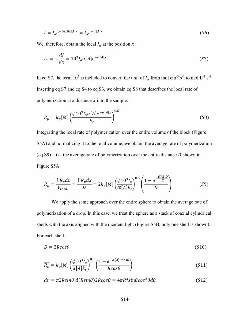
𝐼 = 𝐼𝑜𝑒−𝑙𝑛10𝜀[𝐴]𝑥 = 𝐼𝑜𝑒−𝛼[𝐴]𝑥 (𝑆6) We, therefore, obtain the local 𝐼𝑎 at the position 𝑥:
𝐼𝑎 = −𝑑𝐼
𝑑𝑥= 103𝐼𝑜𝛼[𝐴]𝑒−𝛼[𝐴]𝑥 (𝑆7)
In eq S7, the term 103 is included to convert the unit of 𝐼𝑎 from mol cm-3 s-1 to mol L-1 s-1.
Inserting eq S7 and eq S4 to eq S3, we obtain eq S8 that describes the local rate of
polymerization at a distance 𝑥 into the sample:
𝑅𝑝 = 𝑘𝑝[𝑀] (𝜙103𝐼𝑜𝛼[𝐴]𝑒−𝛼[𝐴]𝑥
𝑘𝑡)
0.5
(𝑆8)
Integrating the local rate of polymerization over the entire volume of the block (Figure
S5A) and normalizing it to the total volume, we obtain the average rate of polymerization
(eq S9) – i.e. the average rate of polymerization over the entire distance 𝐷 shown in
Figure S5A:
𝑅𝑝̅̅̅̅ =
∫ 𝑅𝑝𝑑𝑣
𝑉𝑡𝑜𝑡𝑎𝑙=
∫ 𝑅𝑝𝑑𝑥
𝐷= 2𝑘𝑝[𝑀] (
𝜙103𝐼𝑜
𝛼[𝐴]𝑘𝑡)
0.5
(1 − 𝑒−
𝛼[𝐴]𝐷2
𝐷) (𝑆9)
We apply the same approach over the entire sphere to obtain the average rate of
polymerization of a drop. In this case, we treat the sphere as a stack of coaxial cylindrical
shells with the axis aligned with the incident light (Figure S5B, only one shell is shown).
For each shell,
𝐷 = 2𝑅𝑐𝑜𝑠𝜃 (𝑆10)
𝑅𝑝̅̅̅̅ = 𝑘𝑝[𝑀] (
𝜙103𝐼𝑜
𝛼[𝐴]𝑘𝑡)
0.5
(1 − 𝑒−𝛼[𝐴]𝑅𝑐𝑜𝑠𝜃
𝑅𝑐𝑜𝑠𝜃) (𝑆11)
𝑑𝑣 = 𝜋2𝑅𝑠𝑖𝑛𝜃 𝑑(𝑅𝑠𝑖𝑛𝜃)2𝑅𝑐𝑜𝑠𝜃 = 4𝜋𝑅3𝑠𝑖𝑛𝜃𝑐𝑜𝑠2𝜃𝑑𝜃 (𝑆12)

S15
We, then, obtain Eq S13 that describes the average rate of polymerization of a
sphere:
𝑅𝑝𝑠̅̅ ̅̅ =
∫ 𝑅𝑝̅̅̅̅ 𝑑𝑣
𝑉𝑡𝑜𝑡𝑎𝑙
= 𝑘𝑝[𝑀] (𝜙103𝐼𝑜
𝛼[𝐴]𝑘𝑡)
0.53
𝑅∫ (1 − 𝑒−𝛼[𝐴]𝑅𝑐𝑜𝑠𝜃)𝑠𝑖𝑛𝜃𝑐𝑜𝑠𝜃𝑑𝜃
𝜋
20
= 𝑘𝑝[𝑀] (𝛼[𝐴]𝜙103𝐼𝑜
𝑘𝑡)
0.5
[3
𝛼[𝐴]𝑅(
1
2+
𝑒−𝛼[𝐴]𝑅
𝛼[𝐴]𝑅+
𝑒−𝛼[𝐴]𝑅 − 1
(𝛼[𝐴]𝑅)2)] (𝑆13)
In eq S13, superscript s to denote a sphere and 𝛼 is defined as 𝑙𝑛10𝜀. Eq S13 is an exact
equation to describe average rate of polymerization of a drop; it will – under certain
conditions as discussed below – reduce to a form that is independent on the radius of the
sample drop, R, and help simplify the experimental procedures with which to study the
kinetics of polymerization.
We define 𝐾′ as the term in the bracket in eq S13
𝐾′ =3
𝛼[𝐴]𝑅(
1
2+
𝑒−𝛼[𝐴]𝑅
𝛼[𝐴]𝑅+
𝑒−𝛼[𝐴]𝑅 − 1
(𝛼[𝐴]𝑅)2) (𝑆14)
We show that eq S14 will approach one when 𝛼[𝐴]𝑅 is sufficiently small. Let
𝑦 = 𝛼[𝐴]𝑅, we obtain Eq S15:
lim𝑦→0
3
𝑦(
1
2+
𝑒−𝑦
𝑦+
𝑒−𝑦 − 1
𝑦2) = lim
𝑦→0
3𝑦2 + 6𝑦𝑒−𝑦 + 6𝑒−𝑦 − 6
2𝑦3 (𝑆15)
Eq S15 is in an indeterminate form – i.e. 0/0 when y approaches zero; its limit can be
calculated following the L'Hospital's rule.
lim𝑦→0
(3𝑦2 + 6𝑦𝑒−𝑦 + 6𝑒−𝑦 − 6)′
(2𝑦3)′= lim
𝑦→0
(1 − 𝑒−𝑦)′
𝑦′= lim
𝑦→0𝑒−𝑦 = 1 (S16)
S16
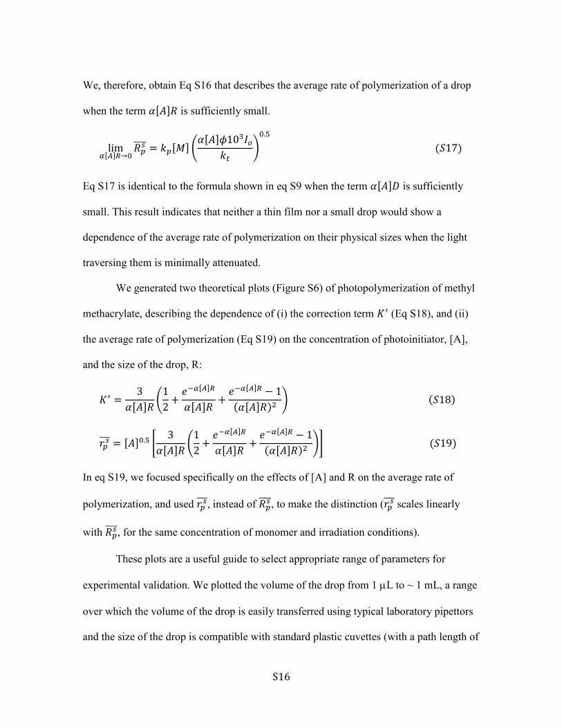
We, therefore, obtain Eq S16 that describes the average rate of polymerization of a drop
when the term 𝛼[𝐴]𝑅 is sufficiently small.
lim𝛼[𝐴]𝑅→0
𝑅𝑝𝑠̅̅̅̅ = 𝑘𝑝[𝑀] (
𝛼[𝐴]𝜙103𝐼𝑜
𝑘𝑡)
0.5
(𝑆17)
Eq S17 is identical to the formula shown in eq S9 when the term 𝛼[𝐴]𝐷 is sufficiently
small. This result indicates that neither a thin film nor a small drop would show a
dependence of the average rate of polymerization on their physical sizes when the light
traversing them is minimally attenuated.
We generated two theoretical plots (Figure S6) of photopolymerization of methyl
methacrylate, describing the dependence of (i) the correction term 𝐾′ (Eq S18), and (ii)
the average rate of polymerization (Eq S19) on the concentration of photoinitiator, [A],
and the size of the drop, R:
𝐾′ =3
𝛼[𝐴]𝑅(
1
2+
𝑒−𝛼[𝐴]𝑅
𝛼[𝐴]𝑅+
𝑒−𝛼[𝐴]𝑅 − 1
(𝛼[𝐴]𝑅)2) (𝑆18)
𝑟𝑝𝑠̅̅̅ = [𝐴]0.5 [
3
𝛼[𝐴]𝑅(
1
2+
𝑒−𝛼[𝐴]𝑅
𝛼[𝐴]𝑅+
𝑒−𝛼[𝐴]𝑅 − 1
(𝛼[𝐴]𝑅)2)] (𝑆19)
In eq S19, we focused specifically on the effects of [A] and R on the average rate of
polymerization, and used 𝑟𝑝𝑠̅̅̅, instead of 𝑅𝑝
𝑠̅̅̅̅ , to make the distinction (𝑟𝑝𝑠̅̅̅ scales linearly
with 𝑅𝑝𝑠̅̅̅̅ , for the same concentration of monomer and irradiation conditions).
These plots are a useful guide to select appropriate range of parameters for
experimental validation. We plotted the volume of the drop from 1 L to ~ 1 mL, a range
over which the volume of the drop is easily transferred using typical laboratory pipettors
and the size of the drop is compatible with standard plastic cuvettes (with a path length of

S17
1 cm) used for density measurements. We plotted the concentration of the photoinitiator
from ~mM to sub M, a range over which the kinetics of polymerization of a drop is not
too slow to be monitored or not overly complicated by nonlinear photoinitiations at high
concentrations of photoinitiators.

S18
Table S1 Hydrophobic organic solvents and monomers that could be used as density
standards
Name Density
reported by
the vendor or
in literature
Density
measured using
a balance and a
gas-tight syringe
Reference
hexyl methacrylate 0.863 0.878 sigmaaldrich.com n-octadecyl methacrylate 0.864 0.858 toluene 0.865 -- sigmaaldrich.com 1,2,3,4-tetramethylbenzene 0.9052 -- 5 methyl methacrylate 0.936 0.932 sigmaaldrich.com 4,N,N-Trimethylaniline 0.937 -- sigmaaldrich.com 4-methylanisole 0.969 -- sigmaaldrich.com anisole 0.993 -- sigmaaldrich.com fluorobenzene 1.025 -- sigmaaldrich.com 3-chlorotoluene 1.072 -- sigmaaldrich.com chlorobenzene 1.107 -- sigmaaldrich.com 2-nitrotoluene 1.163 -- sigmaaldrich.com nitrobenzene 1.196 -- sigmaaldrich.com dichloromethane 1.325 -- sigmaaldrich.com 1,1,2-trichlorotrifluoroethane 1.575
-- sigmaaldrich.com
1,2-dibromoethane 2.180 -- sigmaaldrich.com dibromomethane 2.477 -- sigmaaldrich.com tribromomethane 2.8910 -- 5

S19
Table S2 Calculating the density of a polymerizing sample
Component Density1 Mass2 Volume
Monomer 𝜌𝑚 (1 − 𝑥)𝑚1 (1 − 𝑥)𝑚1
𝜌𝑚
Polymer 𝜌𝑝 𝑥𝑚1 𝑥𝑚1
𝜌𝑝
Initiator 𝜌2 𝑘2𝑚1 𝑘2𝑚1
𝜌2
Solid3 𝜌3 𝑘3𝑚1 𝑘3𝑚1
𝜌3
1: For a given experiment, all density values are assumed to be known (on the basis of the
reported values in the literature or by the vendor, or the experimental values measured
independently using MagLev), and used for calculations.
2: 𝑚1 is the starting mass of the monomer. 𝑥 is the fractional conversion of the monomer
during polymerization. 𝑘2 and 𝑘3 are mass ratios of the corresponding component to the
monomer, and are experimentally adjustable.
3: Solid materials used in this study were aramid, glass fiber, and carbon fiber. This
calculation applies equally to solvents when used to dissolve the reactants. 𝑘3 = 0 for
polymerization in the absence of a solid material or a solvent.

S20
Figure S1 A MagLev device used in this study. A pair of like-poles facing magnets
(Length x Width x Height: 25.4 mm x 25.4 mm x 50 mm, face-to-face separation: 25.0
mm) were mechanically secured using 3D-printed plastic parts and stainless steel rods
and nuts (both interact weakly with magnets, and thus, minimally disturb the magnetic
field between the two like-poles). A drop of 3-chlorotoluene stably levitated in an
aqueous solution of 0.5 M MnCl2 , and did not physically touch the wall of the plastic
cuvette. A ruler with mm scale markings was placed on the side to measure the levitation
height of the drop.
S21
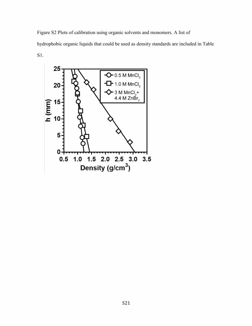
Figure S2 Plots of calibration using organic solvents and monomers. A list of
hydrophobic organic liquids that could be used as density standards are included in Table
S1.

S22
Figure S3 A demonstration of the use of MagLev to monitor the reaction progress of
suspension polymerization of benzyl methacrylate. We carried out suspension
polymerization in a 50-mL flask equipped with a magnetic stir bar and controlled the
reacting temperature using an oil bath. We used 1% (wt%) of poly(vinyl alcohol) in water
to help stabilize the monomer drops. To monitor the progress of reaction, a small aliquot
of the suspension (~500 L) was periodically removed (sample was carried out with a
laboratory pippetor), cooled, and transferred to a MagLev device for density
measurement. We used the standard MagLev device described in our previous studies1 to
perform this demonstration (two indistinguishable NdFeB magnets, Length x Width x
Height=50.8 mm x 50.8 mm x 25.4 mm, placed with like-poles facing at a distance of
45.0 mm). The density – and also the drop size – increased as polymerization reaction
proceeded. Occasionally, small air bubbles were trapped in the polymeric particles (e.g.
the particles towards the center of the cuvette at 25 min and 30 min), and thus, decreased
the apparent densities of these particles.

S23
Figure S4 (A) Spectrum of UV irradiation. (B-C) Spectra of absorption of the
paramagnetic medium, the liquid of monomer (methyl methacrylate, MMA), the
photoinitiator dissolved in the MMA (0.05%, wt%), anisole, and the photoinitiator
dissolved in anisole (0.05%, wt%). We performed the measurements using standard-sized
quartz cuvettes with a 10-mm light path in a UV/vis spectrometer.
A B C

S24
Figure S5: Theoretical model to derive the average rate of polymerization of a drop (A)
The geometry used to derive the average rate of photopolymerization for a block. (B) The
geometry used to derive the average rate of polymerization for a spherical drop.

S25
Figure S6 Dependence of the correction term (top panel) and the average rate of
polymerization (bottom panel) on the concentration of the monomer and the radius of the
drop. The exact equations used to generate the plots are given in eq S18 and eq S19. The
absorption coefficient α for the photoinitiator, 2,2-dimethoxy-2-phenylacetophenone, was
experimentally determined to be 1188 M-1 cm-1 in pure methyl methacrylate.
1.0
2.3
5.1
11
.4
25
.6
57
.7
12
9.7
29
1.9
65
6.8
14
77
.9
0 . 2 5 0
0 . 1 4 8
0 . 0 8 8
0 . 0 5 2
0 . 0 3 1
0 . 0 1 8
0 . 0 1 1
0 . 0 0 6
0 . 0 0 4
0 . 0 0 2
[A
] (
M)
V o l u m e o f t h e d r o p ( L )
0 . 2
0 . 4
0 . 6
0 . 8
1 . 0
1.0
2.3
5.1
11
.4
25
.6
57
.7
12
9.7
29
1.9
65
6.8
14
77
.9
0 . 2 5 0
0 . 1 4 8
0 . 0 8 8
0 . 0 5 2
0 . 0 3 1
0 . 0 1 8
0 . 0 1 1
0 . 0 0 6
0 . 0 0 4
0 . 0 0 2
[A
] (
M)
V o l u m e o f t h e d r o p ( L )
0
0 . 0 5
0 . 1 0
0 . 1 5
K’ from Eq S18
𝑟𝑝𝑠̅̅̅ from Eq S19

S26
Figure S7 Comparison of fractional conversions of methyl methacrylate in
photopolymerization using MagLev and 1H NMR.
S27
Figure S8. Overlaid 1H NMR spectra of sample drops (dissolved in deuterated
chloroform) removed from the aqueous suspending media placed in the MagLev device
at specified time points. Each spectrum is successively offset by 0.1 ppm. See appended
spectra at 0 min and 80 min for assignments of peaks to protons in the monomer and in
the polymer.

S28
1H NMR Spectra of polymerizing drops containing the monomer, methyl methacrylate,
and the photoinitiator, 2,2-dimethoxy-2-phenylacetophenone. See spectra at 0 min and 80
min for assignments of peaks.
Time t = 0 min

S29
Time t = 20 min
600Sch20min.espDate: Nov 18 2017Number of Transients: 100
9 8 7 6 5 4 3 2 1 0
Chemical Shift (ppm)
0
0.1
0.2
0.3
0.4
0.5
0.6
0.7
0.8
0.9
1.0
Norm
alized Inte
nsity
3.220.563.021.031.00
water
CDCl3
6.1
1
5.5
7
3.7
63.6
0 3.2
2
1.9
51.8
2
1.2
5
1.0
20.8
5

S30
Time t = 40 min
600Sch40min.espDate: Nov 18 2017Number of Transients: 100
9 8 7 6 5 4 3 2 1 0
Chemical Shift (ppm)
0
0.1
0.2
0.3
0.4
0.5
0.6
0.7
0.8
0.9
1.0
Norm
alized Inte
nsity
3.391.513.001.031.00
water
CDCl3
6.1
1
5.5
7
3.7
63.6
0
3.2
2
1.9
51.8
2
1.2
5
1.0
20.8
5
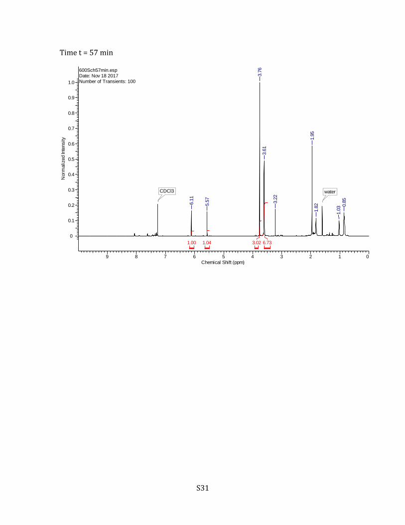
S31
Time t = 57 min
600Sch57min.espDate: Nov 18 2017Number of Transients: 100
9 8 7 6 5 4 3 2 1 0
Chemical Shift (ppm)
0
0.1
0.2
0.3
0.4
0.5
0.6
0.7
0.8
0.9
1.0
Norm
alized Inte
nsity
6.733.021.041.00
waterCDCl36.1
1
5.5
7
3.7
63.6
1
3.2
2
1.9
51.8
2
1.0
3 0.8
5

S32
Time t = 80 min

S33
Figure S9 Changes in shape of the polymerizing drops (A) A drop (43.3 L) of methyl
methacrylate with dissolved photoinitiator levitated in an aqueous solution of 0.5 M
MnCl2. (B-E) Changes in the ratio of width to height over time for polymerizing drops
having different volumes.

S34
Figure S10 Changes in temperature of a polymerizing drop in a MagLev device
monitored with a thermocouple. (A) A small drop (drop 2, ~3.7 L) of methyl
methacrylate containing photoinitiator (5%, wt%) was placed on the tip of a
thermocouple, and a second drop (drop 1, ~1.3 L) levitated in the suspending medium
(0.5 M MnCl2). The levitation heights of drop 1 were marked by the white arrows, and
the adherent drop 2 was marked by the black arrowhead. The UV lamp sat to the right
side of the cuvette. (B) Side view of the adherent drop supported on the tip of a
thermocouple. Drop 1 was not shown. (C) Fractional conversion of methyl methacrylate
in drop 1 (filled circles) indicates the progress of polymerization in drop 2. The
temperature of the polymerizing drop 2 (open circles) was plotted on y-axis on the right.

S35
Figure S11 Levitation heights of polymerizing drops (left) and fractional conversions of
monomer in polymerizing drops having different volumes (right).

S36
References
(1) Mirica, K. A.; Shevkoplyas, S. S.; Phillips, S. T.; Gupta, M.; Whitesides, G. M. J.
Am. Chem. Soc. 2009, 131, 10049-10058.
(2) Nemiroski, A.; Soh, S.; Kwok, S. W.; Yu, H. D.; Whitesides, G. M. J. Am. Chem.
Soc. 2016, 138, 1252-1257.
(3) Winkleman, A.; Perez-Castillejos, R.; Gudiksen, K. L.; Phillips, S. T.; Prentiss,
M.; Whitesides, G. M. Anal. Chem. 2007, 79, 6542-6550.
(4) Odian, G. Principles of polymerization; 4th ed.; John Wiley & Sons, Inc.,
Hoboken, New Jersey., 2004.
(5) Mackay, D.; Shiu, W.-Y. Handbook of Physical-Chemical Properties and
Environmental Fate for Organic Chemicals; 2nd ed.; CRC press, Taylor & Francis
Group, LLC: Boca Taton, FL, 2006.
Top Related