


Languages
Pages
Legal


MACROECONOMIC DETERMINANTS OF MANUFACTURED EXPORTS IN KENYA
M.A.
\
, 1RESEARCH PAPER
BY
U N I V E R S I T Y O F N A I R O B I EAST AFRICANA COLLECTION
MUNGA BOAZ OMORI
University of NAIROBI Library
0472824 2
Research Paper submitted to the Department of Economics, University of Nairobi, in Partial fulfillment of the requirements for the degree of Master of Arts in Economics.
November 2001

DECLARATION
This research paper is my original work and has not been presented for a degree in any other university.
Munga Boaz Omori
This research paper has been submitted for examination with our approval as university supervisors.
Dr. H. Ommeh
S'. il-2oo|

DEDICATION
I dedicate this work to my mum and dad
U N I V E R S I T Y O F N A I R O B I EAST AFRICANA COLLECTION
111

ACKNOWLEDGEMENTS
I would like to thank the African Economic Research Consortium (AERC) for its
financial and academic support. I benefited immensely from the Collaborative Master of
Arts Programme (CMAP), which to a large extent renewed the thought of studying
international trade issues.
I am grateful to my supervisors; Dr. H. Ommeh and D.O. Abala, for their incisive
comments that helped shape this paper. Other thanks go to Prof. F.M. Mwega who gave
thought provoking ideas in the initial stages of the paper. My colleagues (M.A class
2000) receive my thanks for their helpful comments and suggestions. Many thanks go to
my kith and kin who tolerated my aloofness.
As the author, I alone do bear the responsibility for this work, that is, its contents and
remaining errors.
Munga B. Omori
IV
TABLE OF CONTENTS
ACKNOWLEDGEMENTS--------------------------------- ivLIST OF ACRONYMS----------------------- ,-------------- viiABSTRACT------------------------ ,-------------- viiiCHAPTER ONE-------------------------------------- 1
INTRODUCTION------------------------------ 11.1 Historical overview of exports------------------ 21.2 Export policy issues------------ ,---------------- 51.3 Structure and composition of exports---------- 71.4 Statement of the problem------------------------- 81.5 Questions of the study---------------------------- ----------------- 101.6 Objectives of the study--------------------------- 101.7 Justification of the study ------------------------ ----------------- 111.8 Organization---------------------------------------------------- 11
CHAPTER TWO--------------------------------------- 12LITERATURE REVIEW — ----- 12
2.1 Theoretical aspects------------------------------------ 122.1.1 Changes in demand---------------------------- /•--------------- 142.1.2 Changes in supply----------------------------- 142.1.3 Dynamic effects--------- ----------------------- 16
2.2 Empirical literature—------------------------------ ---------------- 172.3 Overview of the literature---------------- 21
CHAPTER THREE----------------------------------- 22METHODOLOGY------------------------------ 22
3.1 Model specification--------------------------------- 223.1.1 Export supply----------------------------------- 223.1.2 Export demand---------------------------------- 253.1.3 Dynamic adjustment---------------------- .■--------- 26
3.2 Estimation strategy----------------------------------- ,-------------- 293.2.1 The small country' assumption--------------- 303.2.2 Structural estimates---------------------------- 30
3.3 Data requirements and sources------------------ — * -------------- 31
CHAPTER FOUR----------------------------------------------------33DATA ANALYSIS AND HYPOTHESES-----------------33
4.1 Graphical analysis of the data--------------------------------------334.2 Unit root tests-------------------------- 344.3 Cointegration and ECM modeling-------------------------------- 364.4 Hypothesis of the study---------------------------- 37
CHAPTER FIVE-----------------------------------------------------38PRESENTATION OF RESULTS & INTERPRETATIONS-------- 38
5.1 The small country assumption--------------------------------------405.1.1 The price equation--------------------------------------------- 405.1.2 The quantity equation------------------------------------------41
5.2 Structural estimate--------------------------------------------------- 435.2.1 Export demand estimates (model B)-------------------------435.2.2 Export supply estimates (model B)----------- 465.2.3 Export supply estimates (model A )--------------------------49
CHAPTER SIX--------------------------- 53CONCLUSIONS AND POLICY IMPLICATIONS---- 53
6.1 Conclusions----------------- 536.1.1 Small country assumption-------------------------------------536.1.2 Export demand estimates--------------------------------------536.1.3 Export supply estimates------ ----------------------------- —54
6.2 Policy implications and recommendations — -------------------586.2.1 The small country assumption----- --------------------------586.2.2 Export demand-------------------------------------------------- 586.2.3 Export supply--------------------------- 59
REFERENCES------------------------------------------------------- 61A P P E N D IC E S-— --------------------------- — -------65
VI
BOPsCOMESACPIDCsEACECFDIGDPIMFIPCKETALDCsNTXsOECDRERSALSAPsSDR /SITCSSATOTUKUNCTADWBWPI
LIST OF ACRONYMSBalance of PaymentsCommon Market for East and South African StatesConsumer Price IndexDeveloped CountriesEast African CommunityEuropean CommunityForeign Direct InvestmentGross Domestic ProductInternational Monetary FundInvestment Promotion CentreKenya External Trade AuthorityLess Developed CountriesNon-Traditional ExportsOrganization for Economic Co-operation and DevelopmentReal Exchange RateStructural Adjustment LoanStructural Adjustment ProgrammeSpecial Drawing RightStandard International Trade ClassificationSub-Saharan AfricaTerms of TradeUnited KingdomUnited Nations Conference on Trade and Development World Bank Wholesale Price Index
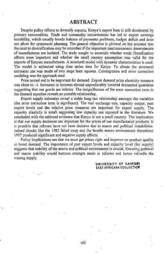
ABSTRACTDespite policy efforts to diversify exports, Kenya’s export base is still dominated by
primary commodities. Trade and commodity concentration has led to export earnings instability, which usually breeds balance of payments problems, budget deficit and does not allow for systematic planning. The general objective is pivoted on the premise that the road to diversification may be smoother if the important macroeconomic determinants of manufactures are isolated. The study sought to ascertain whether trade liberalization efforts were important and whether the small country assumption was valid for the exports of Kenyan manufactures. A structural model with dynamic characteristics is used. The model is estimated using time series data for Kenya. To obtain the structural estimates use was made of two stage least squares. Cointegration and error correction modeling was the approach used.
Price turned out to be important for demand. Export demand price elasticity measure was close to -1. Increases in incomes abroad unpredictably lowered demanded quantities suggesting that our goods are inferior. The insignificance of the error correction term in the demand equation reveals an unstable relationship.
Export supply estimates reveal a stable long run relationship amongst the variables (the error correction term is significant). The real exchange rate, capacity output, past export levels and the relative price measures are important for export supply. The capacity elasticity is small suggesting low capacity use reported in the literature. We concluded, with the adduced evidence that Kenya is not a small country. The implication is that our supply decisions are important for the prices of our manufactured products. It is possible that reforms have not been decisive due to macro and political instabilities. Indeed shocks like the 1982 failed coup and the hostile macro environment thereabout 1997 produced significant and negative supply effects.
Policy implications are that we must get prices right and improve on product quality to boost demand. The importance of past export levels and capacity level (for supply) suggests that stability of the macro and political environment is crucial. Ensuring political and macro stability would buttress attempts made at reforms and hence rekindle the waning supply.
U N I V E R S I T Y O F NAIROBII EAST AFRICANA COLLECTION
Vlll
CHAPTER ONE
INTRODUCTION
In this study manufactured products are as defined in the Standard International Trade Classification
(SITC). Manufactures comprise the commodities in SITC sections 5 (chemicals), 6 (basic
manufactures), 7 (machinery and transport equipment), and 8 (miscellaneous manufactured goods).
Appendix 1 gives a detailed classification of commodities by SITC sections.
Our study topic discriminates micro variables; however, both micro and macro determinants are
perhaps equally important in determining the level of exports of manufactured goods. Roberts, J.M. and
Tybout, J.R. (1997) suggest that the unpredictable effects of macroeconomic conditions and policy
variables on manufacturing exports - can be traced largely to ignored microeconomic characteristics of
manufacturing sectors. Elbadawi and Schmidt - Hebbel (1996) postulate that macroeconomic reforms
may be more important than micro and sectoral policies in terms of their effects on economic
performance in general and on whether countries can avoid development crisis especially following
external shocks. These views strengthen both micro and macro variables.
Less developed countries (LDCs) are generally characterized by a higher ratio of primary products
to manufactured goods in their export bundles than in their import bundles, which has relevance to
potential problems of export instability and terms of trade (TOT) behaviour that the LDCs face in
international trade.
Real prices of the chief agricultural primary commodities exported by developing countries have
fallen steadily since 1960, the fall accelerated in the 1980s.
1
Between 1982 and 1990 world market prices for coffee, cocoa and tea - then three of the developing
world’s major export crop earners fell at an average rate of 11% a year (UNCTAD, 1991). Obote (1981)
concludes that, “the problem is that the production and supply of primary commodities are generally
outpacing consumption and demand, which means that prices are likely to be low. Sizable reduction in
the output of commodities would be needed to raise prices.” This view has relevance today, World Bank
(1998) states that for many agricultural commodities large price declines since mid 1997 were a
reflection more of record world production than of the Asian financial crisis.
Sub-Saharan Africa’s (SSA) importance in global trade has declined substantially over time. In the
1960s the region accounted for 3 per cent of world trade - this has fallen to 1.2 percent today. In the
1980s exports expanded at a rate of 1.8 per cent compared to a world average of 5.3 per cent (World
Bank 1996). This poor performance is postulated to reflect (among others) the slow responsiveness of
exports to the substantial (and contagious) economic reforms that African countries have implemented
in the 1980s and 1990s.
1.1 Historical overview of exports in Kenya.
j
Kenya is also reliant on primary commodity exports and her trade deficit has been widening 1 with
the trend expected to continue (Economic Survey, 2000). The range of exported goods has all along
been narrow [Coffee, tea and petroleum remain by far the dominant commodity exports, (see table 1.1
below) accounting for 48.5 percent of total exports in 1998].
■ The balance of trade deficit increased from K£ 1378 million to K£ 2892 million in 1995. This was 10.2 and 14.9 per cent in relation to GDP at current
Prices, respectively National Development Plan (1997-2001). The trade deficit was put at K£ 3830.40 million in 1998 (Economic Survey, 2000).
2
Export diversification is a recommended policy virtue, but it is riddled with constraints. The constraints
are elaborated in the review of the literature.
Table 1.1: Top three exports as a proportion of Total Exports, %
SITC Item 1980-4 1985-9 1990-4 1995-6 1997 1998
~T\ Coffee 27.6 68.8 22.7 24.7 14.7 11.21A Tea and mate 2.2 1.8 5.1 6.0 21.1 28.8334 Petroleum products 16.3 5.4 4.8 3.4 9.0 8.5
Total 46.1 76 32.6 34.1 44.8 48.5Source: Kenya, Annual Trade Report, various issues.
The country’s manufactured exports may be divided into three groups (WB, 1987). The first group
comprises standardized products such as cement and paper, made in fairly large and modem plants. The
orientation of these goods has been more towards the East African area in recent times. The second
group - products sold mainly outside Africa - comprises exports based on distinctive natural resources.
These include leather, wattle bark extract and woodcarvings. The third group, which comprises about
two thirds of manufactured exports is sold almost entirely in Africa. Chemicals and iron and steel
products feature prominently in this group (World Bank, 1987).
In the 1960s, the manufacturing sector in Kenya saw rapid expansion with textiles and garments,
food, beverages and tobacco as the leading sectors. Import Substitution continued to be the main policy
emphasis. In the 1960s and 1970s, Kenya was classed as an outward industry- oriented country as it had
relatively high exports of manufactured goods. The share of manufactured exports has however declined
, over time, leading Syrquim (1992) to classify Kenya as a ‘balanced’ country as it did not fit easily into
the outward primary, outward industry or inward orientation categories.
Exports of manufactured products comprised only 11.7% of total exports in the 1980s (down from
40% in the 1960s). Except for beverages and tobacco, the proportion of manufactured output exported
by various industries declined in the 1980s. The decline in the share of manufactured exports in total
exports as well as in total output in the 1980s has been attributed to a decrease in exports to the
neighbouring countries, especially- Tanzania where the volume of imports from Kenya had not yet
reached the levels attained before the breakup of the East African Community in 1977; growth in
domestic demand for such products as paper; the anti export bias of the trade policies; and supply
constraints, especially the intermittent shortage of foreign exchange to purchase intermediate inputs
(Sharpley and Lewis 1988). Up to the early 1990s, the performance of manufactured exports had been
poor, their contribution to the country’s total exports having declined to thirteen percent in 1991 from
sixteen percent in 1975.
Manufactured exports have rebounded, however, in the 1990s and comprised 26.6% and 28% of
total exports in 1990-4 and 1995-6, respectively. Nearly all manufactured exports increased their shares
in the 1990s. The authorities attribute this to trade reforms and the depreciation of the Kenya shilling
achieved in the period. Another important source of manufactured export growth was rescue activities
arising from turmoil in neighbouring countries, particularly Somalia and Rwanda (Mwega,
forthcoming). During the period 1990-1999 manufacturing grew by 2.4 percent on average. In 1999
manufacturing grew by only 1.0 percent in real terms (see Economic Survey 2000). A look at the graph
of exports of manufactures (see appendix 2) reveals that the real dollar value of manufactures has been
on a general decline since 1997. A brief discussion of export related policy issues follows.
4
1.2 Export policy issues.
At independence the new Government inherited an industrial policy, which was based on import
substitution (IS). The colonists were preoccupied with the protection of the colony (Kenya) as a
producer of agricultural and other raw materials for England’s manufacturing sector and a ready market
for manufactured goods from Europe. The IS policy was a key influence on the development of the trade
regime of Kenya over the first ten years since independence (the strategies were largely motivated by the
Prebisch - Singer hypothesis of secularly declining TOT). The increasing resort to import licensing is
thought to have been a product of Kenya’s membership of a customs union (the East African
Community) with Tanzania and Uganda, making use of tariffs difficult (WB, 1987). By mid 1970s it
was clear that the IS strategy in Kenya was approaching its limits. Furthermore a major outlet for
Kenya’s manufactured goods, the East African Community (EAC) collapsed.
With the collapse of the regional markets, IS firms started operating at excess capacity and pressure
swelled on the Kenyan Government to increase protection of local manufacturing - many of which were
parastatals. As the import substitution regime progressed, a large bureaucracy was set to implement it,
supervising and implementing import bans and controls, allocating foreign exchange, issuing trade
licenses and such. By the end of 1970s the high cost of import substitution strategy to Kenya’s economy
was already evident. The evidence in Kenya was that manufactured exports were not performing well
and this was partly due to the relative unprofitability of manufactured exports vis -a -vis sale to the
domestically protected market. The fourth development plan (1979 - 83) confirming government’s
policy changes - acknowledged that ‘past industrial growth had been fostered by excessive protection,
^suiting in an industrial sector which was uncompetitive, overly capital intensive in relation to Kenya’s %actor endowments and a heavy net consumer of foreign exchange.’
5
Kenya attempted to transform trade policies (shifting from IS to an export promotion strategy) as
part of Structural Adjustment Programs (SAPs). The WB through the Structural Adjustment Loan (SAL)
facility supported various programs in Kenya. Important policy highlights include:
♦ Export Compensation Act (the first incentive to be enacted) was implemented in 1976. The
scheme (proposed in i974) was designed to provide compensation to offset the import duties paid
on inputs used in the production of exports. Delays in payments and whimsical Changes made to
the subsidy were decisive in making this promotional tool impotent.
♦ Kenya External Trade Authority (KETA) was established in 1976 to strengthen and reorganize
export promotion. The organization was to develop specialized committees in the fields of export
training, handicrafts, trade fairs and exhibitions, trade facilities and publicity. Other important
! institutional bodies include/included; Department of External Trade- established in the 1950s andiii Investment Promotion Centre (IPC)- established in 1982. The effectiveness of KETA and other1 ‘\
i institutional bodies was undermined by the level of resources - both financial and human -1
provided by the Government (Kenya Association of Manufacturers, 1989 p.48).
♦ Tariff reforms were implemented in the 1980s and 1990s. These had some impact in reducing
the effective tariffs (Mwega, 1995).f
♦ In 1983 the Central Bank imposed foreign exchange allocations (these were removed in 1993).
Restrictions were mainly administered through import licensing.
♦ Between 1980 and 1982, the Kenya shilling was devalued by about 20 percent in real terms
measured against the special drawing right (SDR). After this devaluation, the exchange rate
regime was changed to a crawling peg in real terms by the end of 1982. This regime lasted until
1990 when dual exchange rate system was adopted that lasted till October 1993. Kenya adopted
6
in October 1993, an exchange rate policy that allows the nominal exchange rate to fluctuate
freely in accordance with market/economic conditions (Amoko, 1996).
♦ There have been attempts made to strengthen government departments for export promotion
(e.g. the Export Promotion Council).
+ Manufacturing under bond was announced in the sessional paper No. 1 of 1986 and
implemented in 1988. Government officials and manufacturers viewed it as an important step
towards improving incentives for export-oriented manufacturing.
Glenday, G. and Ryan, T.C.I. (2000) comment that since independence Kenya has been through a
process of protecting and controlling its markets that went through a buildup that peaked in early 1980s.
Further it is argued that Kenya has only experienced a truly open trade and exchange rate policy since
the major liberalization of 1993 - 94.
1.3 Structure and composition of exports.
Kenya’s export profile reveals that there have been minimal attempts, or negligible success (or both)
to mutually diversify export markets and products (See table 1.1). Fresh horticultural exports have been
the only positive move towards diversification (Eliud M. and Kimuyu P. 1999).
Africa is currently the principal market for Kenya’s total exports (in 1998 Kenya exported 45 per cent of
its total exports to Africa). Although its share averaged 29% during the period 1987-92 this rose to 34%
in 1993 and has exceeded 43% since 1994. By 1995, the largest African importers of Kenyan goods
were Uganda (32%), Tanzania (25%), Rwanda (7%), Zaire (3%), and Sudan (3%). Apparently, the East
*nd Central African region where Kenya exploits economies of proximity has dominated Kenya’s export
trade within Africa. Exports to Uganda and Tanzania stood at 29.4 per cent of total exports in 1998.
7
Kenya’s second most important market is the European Community (EC). Up to 1993, the EC
dominated Kenya’s export trade, its share varying between 40% and 50% of the total. However by 1994,
this share had fallen to 34%. Between 1994 and 1998 the EC’s share has averaged about 32.4 per cent of
the total exports. Within the EC, United Kingdom (UK) has been the leading importer, followed by
West Germany and Netherlands. Since 1994, there has been a gradual shift from Western Europe as the
principal destination for Kenya’s exports to the African region [Mwega (forthcoming) notes that the
shift may suggest declining competitiveness]. The share of exports going to the Far East and Australia
remained torpid at about 10% of total export trade. Kenya’s share of the export market in W. Europe, E.
Europe, North and South America and Middle East has been stagnant.
1.4 Statement of the problem
Trade liberalization is a central plank of SAPs implemented in Africa and elsewhere. An important
objective of these programs has been to enhance economic growth by increasing exports of
manufactured items. The demand for manufactured commodities as compared to primary commodities
is steadier and less cyclical, so that primary exporters are more subject to terms of trade (TOT) losses
than exporters of manufactured items. Despite policy efforts to diversify exports, Kenya’s export base is
still dominated by primary commodities (see table 1.1). Although the possibility of short run price
increases cannot be ruled out, the long term prospects of rising international prices (for Kenya’s main
primary commodities) are poor given worldwide overproduction and existing stocks. As long as primary
> commodities dominate Kenya’s export sector, its performance is likely to be lacklustre. There is need
therefore for diversification into higher value exports, mainly manufactured products. The way to
diversification may be smoother if important determinants are isolated. Diversification of products and
8
markets is vital since commodity concentration and high trade concentration (revealed in the section
above) lead to export instability. Export instability usually breeds Balance of Payments (BOPs)
problems, budget deficit and does not allow for systematic planning.
In 1993 Kenya effected trade liberalization measures (removal of import licensing, quantitative
restrictions and foreign exchange controls) and the increase in the value of imports that resulted, was
(and is) not matched by a corresponding increase in export earnings {in the year 2000 exports and
imports grew at 9.8 and 20.1 percent respectively (economic survey, 2001)}. There is therefore a need to
have high value exports to provide adequate foreign exchange to stamp out foreign exchange
difficulties, or problems (National Development Plan 1997 - 2001). The government, aware of the
gravity of the problem has pursued liberal policies to promote exportdiversiflcation. However, there has
been little impact on the export trade. This suggests that there are serious constraints to export
development and diversification that need to be investigated with care.
Amongst the studies done so far none has attempted to look at the role of external demand on the
export of Kenyan manufactures. As an example, the real income of Tanzania (a major trading partner)
declined by a third between 1980 and 1985 (see WB, 1987). The ‘small country’ assumption is usually
; used to exclude demand conditions. However, to explain policy performance such changes in foreign!incomes should be taken into consideration.
9

1.5 Questions of the study
This study intends to answer the following questions.
1 .What macroeconomic aspects have impeded (or aided) the supply response of manufactured goods?
2. What is the likely impact of a change in external economic activities (measured by changes in the
incomes abroad) on manufactured export revenues?
3. Have trade liberalization measures been decisive in influencing export levels of manufactured items?
4. Does Kenya have monopoly power over the sale of its manufactures?
U N I V E R S I T Y O F N AI R O BI1.6 O bjectives o f the study east africana collection
The general objective of this study is to analyse the macroeconomic determinants of manufactured
exports from Kenya. The specific objectives of this study are:
1. Capture the effect of ‘external conditions’ on the exports of Kenyan manufactured products. Changes
in ‘external conditions’ will be captured using the weighted GDP of Kenya’s main trading partners.
2. Ascertain the importance of trade liberalization episodes in influencing the size of exports of
manufactured goods (e.g. the trade liberalization episode of 1993 -94).
3. Ascertain whether the small country assumption is appropriate for Kenya in as far as export ofI
manufactures is concerned. In the process the study will calculate multipliers relevant for policy
decisions. These include export volume, export price and export revenue multipliers (elasticities).
1.7 Justification of the study
Policies to diversify the export base have not produced visible difference in the export statistics.
This is in spite of the glorified newer and diverse opportunities brought about by globalization. This
suggests that there are serious constraints to export growth and diversification, which necessitate careful
investigation.
Exports of both primary goods and manufactured goods is an area replete with studies. However
hardly any studies have attempted to capture the effect of changes in external economic activities on
export revenues for developing economies (Kenya included). The findings of this study are expected to
illuminate the policy decisions.
.8 Organization//
The rest of the paper is structured as follows: chapter two reviews relevant literature (both
------ jeoretical and empirical) on the export, of manufactured products. An overview is attempted at the end
i this chapter. Chapter three discusses the model to be used and the estimation strategy. The data type
jd sources are discussed in this section too. The third chapter is concluded by giving the time frame of
| study. Chapter four begins with a graphical analysis of the data, presents the unit root tests and lastly
es the studies hypotheses. Presentation of results is done in the fifth chapter. We wind up the paper
is customary) by giving the conclusions and policy suggestions in chapter six.|f|
\ j
1iiiitf5
CHAPTER TWO
LITERATURE REVIEW
This chapter reviews the theoretical literature on the macroeconomic determinants of exports ii
general. The empirical literature essentially focuses on the literature related to this current study in th<
developing countries before focusing specifically on Kenyan literature.
2.1 Theoretical aspects
The Heckscher-Ohlin (HO) model (a neo-classical model) explains that a country will export thos< / *
commodities in which its most abundant factor is used relatively intensively and import thosf
commodities which incorporate the factors in which it is least endowed (Sodersten, 1995). The HO -
model can be used to explain why LDCs, including Kenya (thought to be capital poor and labour rich
export mainly primary commodities. The earlier Ricardian model of trade (dubbed as a classical model
was silent about why comparative cost ratios differed between countries. Ricardo argued that labou:
productivity differentials between countries brought about trade. The Ricardian theory was based on th<
labour theory of value, which became a subject of great controversy thereafter.
Modern textbook writers discuss exports when the economy is finally ‘opened’ (that is, when the foreigi
sector is introduced). The export function (x), is typically given as,
X = X(P, e)
i
12
The above function states that for a given level of aggregate foreign demand and prices, real exports (X)
will depend on the domestic price level (P) and the exchange rate (e). The relationship is such that real
exports are negatively related to both P and e. Whether the money value of exports (x) rises or falls
depends on the elasticity of foreign demand for exports. More recent works (see Roemer, 1996) analyse
exports as a function of real exchange rates i.e. X = X (pf/p), where:
p = domestic prices
p, = foreign prices.
The negative relationship between real exchange rates and exports is argued to be circumstantial if the
Marshall-Lerner conditions are invoked (effectively making theory ambiguous).
Originally, the theoretical interest was on what role export diversification could play in reducing the
variability of export earnings from the cyclical fluctuations in the International prices of primary
commodities (Mac Bean, 1966; Mac Bean et, al., 1980). Countries that specialized in a narrow range of
primary commodities are currently faced with declining export earnings and a loss in their share of the
International export markets (IMF, 1986).
The trend since 1970 has fashioned a theoretical response, which argues that in a world of changing
demand and supply conditions, international trade should be based on dynamic comparative advantage.
The dynamic elements focused upon are demand and supply changes; risk evasion given imperfect
foresight and changes in commercial policies.
13
2.1.1 Changes in demand
Engel’s law predicts that necessities are income inelastic. As income in the consuming countr
increases, the proportion spent on necessities declines. An exporter facing rising income in the importim
country has to diversify by increasing the proportion of commodities which are income elastic ant
reducing the proportion of necessities in order to realize rising export earnings.
Even if incomes in the importing countries are unvarying, tastes change, and indifference maps shif
over time, with changes in psychological preferences of different generations of customers. This call:
for diversification to generate new exports to cater for the changing, desires and needs. Both income:
and tastes have been changing over time in the European and African markets, which are the mail
destinations of Kenyan exports (IMF, 1987).
2.1.2 Changes in supply
Dynamic comparative advantage calls for diversification to develop new exports as the country
adjusts its productive structure to changes in domestic resource endowments such as new skills fron
education or better land utilization that nullifies diminishing returns, or changes in productior
\ technology and input mix, or changes in the availability of imported inputs in response to the foreigr1; exchange constraint. Even if resource base and inputs remained unchanged, a country’s internationa|j , .i competitiveness changes in response to the domestic macroeconomic environment, such as the rate oi! . 1 -
inflation and the competitiveness of other suppliers of identical commodities. Such changes will be
reflected in movements in the real effective exchange rate, which signals a reallocation of resources intcia new diversity of exports.j! Complete specialization, especially in primary commodities with long gestation periods such as treei
Cr°ps, creates an inflexible export structure in the short-run. Even if the price elasticities of supply oi
these commodities turn out to be large in the long run, a country cannot adjust to short-run booms oi
14
decline in international prices. More importantly, it is also difficult to predict whether such price
fluctuations are short-run and cyclical or whether they represent a secular trend that requires a re
allocation of resources.
Several well known theories explain the phenomenon of irreversibility in export supply
relationships, sometimes called export hysteresis. If incumbent exporters incur sunk start up costs - they
find it more profitable to continue selling abroad than do identical firms without exporting experience.
Firm level studies (among Kenyan exporters) find that sunk costs are important in determining firms
response to export incentives, implying that even if the exchange rate were to increase profitably the
response may be limited unless profitability crosses the threshold at which firms are willing to invest in
exporting (see Mwega forthcoming).
On the policy front this implies that a temporary devaluation, which induces new entry, may
permanently increase the number of exporters. Similarly temporary unfavourable conditions for
exporters can permanently reduce the export base (Baldwin 1988; Krugman 1989). Further the tendency
of producers to ‘stay put’ in the face of exchange rate fluctuations is likely to increase with uncertainty
about future exchange rates (Dixit 1989). Managers want to avoid repeatedly bearing start - up costs. So,
if they can learn something about the medium term future by waiting to see how events unfold, they may
do so.
Obstacles in the LDCs that prevent the appropriate supply response are related to deep-seated
development problems such as the lack of rapid transport to deliver these commodities fresh to the
markets, or lack of processing capacity to preserve them in the form that lengthens their shelf-life. The
association between industrial and export capacity becomes relevant in this case: as industrial capacity
grows, the evidence over the last fifteen years shows that processing capacity itself, plus the related
15
infrastructure, increase the country’s flexibility to process and supply agricultural commodities with
high income and price elasticities of demand (IMF 1987 and Harrylyshyn, 1990).
2.1.3 Dynamic effects
Expansion of output brought about by access to the large international markets permits the LDC to
take advantage of economies of scale. Other dynamic influences of trade on economic development
arise from increased investment resulting from the changes in the economic environment, the increased
dissemination of technology into the developing country (e.g. the product cycle), exposure to new and
different products.
International trade theory postulates that developing countries perceived as possessing abundant/
labour relative to capital should have a comparative advantage in labour intensive products in their trade
with the rest of the world. However, low skill levels observed in Kenya’s manufacturing are likely to
limit the country’s comparative advantage to primary products and away from manufactured products
(Kimuyu 1998).
16
2.2 Empirical literature.
The general view is that the factors inhibiting export growth and diversification of exports are
similar to those explaining Africa’s low growth. They include human resources (including healthy and
skilled workers), factors that affect transactions costs (including governance and infrastructure services),
policies that ensure a stable and competitive macroeconomic environment, and geographic factors (see
WB 2000). This section will dwell on factors related to the macro economy.U N I V E R S I T Y O F N A I R O B I
Indeed, the important variables that explain the movements in the Iev6ft6f d£{5ttft$ffci‘£p<blieyTalated
variables. The main instruments of trade policy are trade taxes, import and export taxes and varieties of
quantitative restrictions on trade. These vary from country to country. One such factor given prominence
in the literature is the exchange rate (ER). The pro - exchange rate arguments may be summarized by/ •
the thoughts of Helleiner (1986). He notes, “so far, the keys to successful expansion of exports seem to
have been realistic and stable exchange rates and sustained governmental support, not import/
liberalization and laissez - faire”. He further argues that raising the quality of the public sector
management may be more important than privatizing public enterprises or liberalizing markets.
Mwega (forthcoming) assesses the extent of response of non-traditional exports (NTXs) to the real
exchange rate and trade liberalisation policies in Kenya (60% of the NTXs2 are manufactures). His
findings are that the real exchange rate (RER) coefficients are insignificant (at the 5 percent level) and
suggest that the RER has not played a significant role in the promotion of NTXs in Kenya. The
explanatory variables used in this study were, real GDP, the bilateral RER, a lagged value for NTX
volume, and trade liberalization episodes.
In mwega’s study NTXs are defined as including merchandise exports accounting for less than 3 percent of total exports in the base year.
17
It is noted that the ability of exporters to respond to ER and trade liberalisation policies will depend on
non-price variables. Mwega gives four broad constraints.These include; availability of finance,
infrastructural inadequacies with respect to transportation, water, energy, waste disposal, and security.
Another constraint is lack of access to external markets arising from ignorance, poor quality of products,
lack of interest (and experience) to sell abroad.
The exchange rate is also affected by the policy stance of the government. This is exemplified by
the argument of Keesing on the ER and policy performance in protection. Keesing (in Meier and Steel,
1989) argues that if a country prefers high protection and direct control, a characteristic of several SSA
countries (probably until recently), ‘this in itself will push the exchange rate in a direction that
discourages exports and natural, unassisted import substitution. Conversely if a country avoids any but
the mildest protection, the resulting exchange rate will be more favourable to exports and make strong
protection less necessary’.
Roberts M.J. and Tybout J.R. (1997) studied export booms among many firms in developing
countries (concentrating on microeconomic aspects) 3. Their study revealed that firms that were already
exporting before the export booms did not dramatically adjust export volumes in response to
devaluation. The explanations given for the response include demand elasticities that are not large, risk
averse behaviour and near full capacity utilization. These explanations varied from one country to
another in importance.
Several studies considered the effect of the RER uncertainty on exports. Using a simple risk model
Caballero R.J. and Corbo V. used data from six developing countries4 and found that the empirical
relationship (between RER uncertainty and exports) is strongly negative - contrary to the ambiguity of
3. This study was conducted among firms in Morocco, Mexico and Colombia.4. The study used data from Chile, Colombia, Peru, Philippines, Thailand and Turkey.
18
the theory. Several studies that have shown a negative relation between RER volatility and exports are
given; these include Behrman 1976 on Chile, Diaz - Alejandro 1976 on Colombia, Coes 1979 on Brazil
and Paredes 1986 on Peru.
There is a fair measure of consensus that the Capacity to produce, usually proxied by GDP is
positive and significant (see Mwega (forthcoming), and Moran 1988). In a study of local firms, the
Regional Programme on Enterprise Developed (RPED) over 1991-4. Bigsten et al. (1998) find that most
(71 per cent) of the large firms in the RPED survey export; hence the problem is not enabling them to
enter the external markets but understanding why they export relatively so little - on average less than 30
per cent of their output. Of the reporting firms, exporting firms had substantially less excess capacity
(44.8 per cent) on the one shift basis than non -exporting firms (61.1 per cent). Overall 85 per cent of
firms were operating below capacity, and cited, as explanations, lack of demand (71.7 per cent) high
cost of credit (34.2 per cent), lack of credit facilities (15.8per cent), expensive labour (13.2 per cent),
shortage of foreign exchange (7.9 per cent), and other factors such as dumping (58.3 per cent).
Wagacha (2000) analyses the determinants of export performance and the role of relative prices.
Total exports regression analysis results indicated that Kenya’s total exports responded to three key
explanatory variables. These were relative export prices, the lagged value of relative export prices and
real wages. Relative export price was defined as the ratio of totaLexport price index, which is proxied by
the price index of non - oil exports to the average weighted CPI.
Policy makers have suggested that protectionism by developed countries has played an important
role (Yeats, 1981). Many development economists however maintain that inappropriate domestic
Policies greatly diminished Africa’s ability to compete internationally. In answering the question, what
has caused Africa’s marginalization in world trade? Yeats A.J. et al. (1998) finds that there is little
,evidence that it was government imposed trade restrictions in OECD markets. Their view is that the
19
share of African exports subject to non - tariff barriers is far lower than that of other developing
countries that launched successful and sustained export - oriented growth. This latter view is buttressed
by the presence of other support schemes. An example is the recent United States’ African Growth and
Opportunity Act (AGOA) designed to remove quotas and tariffs for apparel and textile imports from
SSA countries. Students of the region (Jonsson and Subramanian (2000); Coe and Hoffmaister (1998)}
argue that among other factors, it is trade restrictions imposed by SSA countries that is responsible for
the poor trade performance in manufactures and other exports. Unilateral trade liberalization by SSA
countries is one of their policy implications.
A study by UNCTAD (1986) showed that, for a sample of developing countries that had
successfully launched an export trade in processed commodities, government support in financing
necessary transport, storage and other infrastructure, in training and research and development facilities,
and in quality control standards, marketing coordination and gathering of marketing intelligence - had
played a crucial role. There was also some evidence that control over marketing and distribution
channels by transnational corporations had been; for certain processed commodities, an important
obstacle to expanded sales by producers in developing countries.
The size of the domestic market for processed products (forms) is likely to constitute a key
constraint on the ability of small, less diversified economies to export processed commodities on a
competitive basis. This explains the widespread discussions on regional integration efforts. We may not
exhaust all the determinants discussed empirically, however, foreign direct investment (FDI) is one
factor that deserves mention. FDI-led restructuring contributed enormously to an impressive expansion
ln Hungarian exports, which was crucial in successfully tackling of what might have been a serious
®OPs crisis in 1995 (Kaminski and Riboud, 2000). The FDI in Kenya has remained devoid of decisive
changes in size.
20
The literature reviewed above reveals that RER might not have played an important role in Kenya
(see Mwega). For total exports relative export prices and real wages have been shown to be significant.
Domestic capacity (a supply factor) was important. No empirical measures were found for the foreign
income elasticity of export demand for Kenya on manufactures. Mwega reports that the trade
liberalization episode of 1993-94 was significant for NTXs, sixty per cent of which were manufactures.
2.3 Overview of the literature
21
CHAPTER THREE
METHODOLOGY
This chapter is primarily concerned with the theoretical presentation of a model, which can be used
as a framework to test the important macro-determinants of manufactured exports m Kenya. W e first
present a simple structural model for export demand and supply and develop and discuss its dynamic
characteristics. We then show how the estimations will be done. The chapter ends with a discussion of
data requirements (and sources and the motivation for its use).
3.1 Model specification
This section presents a simple structural model6 identifying separately the manufactured products
export supply and demand equations.
3.1.1 Export supply
The supply design assumes that producers base their production decisions on two main factors:
domestic capacity and the relative profitability of producing manufactured exports vis-a-vis producing
other goods (including other exports, import substitutes, and home goods).
Measurement of domestic capacity presents great difficulties because sector wise capital stock data
are usually not available. Three measures have been predominantly used in the literature as proxies for
domestic capacity. The first, assumes that time or any other trend factor (e.g. trend Gross Domestic
22
Product, y*) can be taken as an indicator of domestic capacity (Bond 1985). This measure implicitly
assumes that domestic resources are mobile across sectors (and also mobile across borders). A second
measure is a capacity utilization index. This is normally defined as deviations from trend output, y-y*.
This approach is equivalent to adding aggregate output (y) as an additional explanatory variable. The
last measure assumes that a sector wise production index can be used as a proxy for domestic capacity
(Balassa and others 1986). This measure has been criticized on the grounds that the production and
export of industrial goods are jointly determined and are both affected by demand factors. Thus
industrial production cannot be assumed to be exogenous in the structural estimation of an export model
(Faini 1985 in Moran 1988).• /
To measure relative profitability, two separate measures of price effects are used. These are:
(1) The real exchange rate (RER), which indicates the relative profitability of producing tradables (T)
versus non-tradables (NT). For measurement purposes the RER = PT/PNT where; PTt = Price of
tradables, in U.S. dollars, calculated as the ratio of value added in current and constant dollars
originating in manufacturing, agriculture, and mining, obtainable from the World Banks National
Accounts database.
PNT = PHt = Price of home goods (non - tradables), in U.S. dollars, calculated as the ratio of value
added in current and constant dollars originating in the remaining sectors (and including construction,
electricity, and private and government services). This is usually proxied by the CPI.
Tradables are goods and services traded across countries borders. If data for PT and PNT are not
available as is defined above, this study will employ a proxy for the RER. A suitable proxy is,
RER = e*WPI/CPI
Where;
e = nominal exchange rate,
23
WPI = Wholesale price index in the country’s main trading partners. WPI (if used) will be accordingly
weighted by the export price index, and
CPI = Consumer price index.
The ratio of manufactured exports prices to other tradable goods prices (PX/PT), which indicates the
profitability of exporting manufactured items relative to other traded goods (thus influencing the share
of manufactured exports in total exports).
A linear version of the export supply equation can be written in the form:
x; = a0 + al(PX/PT)t + a2(PH/PT)t+a3y,........................................ (1)
(Xi > o, ot2 < 0, and 0,3 > 0U N I V E R S I T Y O F N A I R O B I
Where: EAST AFRICANA COLLECTION
x’= Manufactured exports [standard International Trade. Classification [SITC 5 to 9] in constant
dollars: The value data are obtainable from national sources.
PXt = Manufactured export unit value index, in current U.S. dollars.
PTt and PNT (PHt) are as defined above.
y*= Capacity output (Capacity output is proxied by GDP at market prices in constant dollars,
obtainable from the World Banks National Accounts database).
All variables are expressed in logarithms. Caveats about the export supply equation (1) should be
noted.
Price indexes will reflect border prices, but exclude the effective taxes and subsidies received (or paid)
by local producers and consumers. This exclusion of domestic taxes and subsidies (due to lack of
relevant data) probably would limit the price responsiveness of the export estimates obtained here.
24
The proxy variable used for domestic capacity (trend GDP) is also correlated with other structural
effects which tend to evolve slowly - such as “learning by doing,” entrepreneurial talent, and the
quality of infrastructure (particularly in transportation and communications).
The model developed here can only be understood in partial equilibrium terms in order to justify the
exogeinity of the RER in the export supply equation.
3.1.2 Export demand.
The export demand specification assumes that external buyers make their decisions on the basis of
relative prices and the growth of external demand.
Relative prices are measured by the ratio of a country’s manufactured export prices to the price of
manufactured exports in World markets, PX/PXW.
The real scale variable, y ”, captures the growth of external demand for each country, reflected in a
simple weighted average of real economic activity (GDP) for the countries main export markets. It
assumes, implicitly, that the exporting country moves into other markets only with a lag, and hence the
geographic distribution of its exports needs to be considered in the definition of external demand.
A linear version of the demand equation can be written in the form:
xf= f i0+M P X /P X w)l +fi2y : ...................................... -(2)
With: Pi < 0, 02 ^ 0 and
xf = The quantity of manufactured exports demanded.
PX, and t are as defined above.
PX" = World price of manufactured exports, in current U.S. dollars.
25
* * u H i
y"= Index of external demand, calculated as a weighted average of economic activity for the
countries main trade partners.
Both equations (1) and (2) will be written in log linear form and thus constant elasticities will be
assumed. This simplifies the interpretation and has been justified in the context of import behaviour
(Thursby and Thursby 1984).
Both are written in terms of relative prices and hence assume that there is no money illusion on the
part of the producers and consumers of manufactured exports.
3.1.3 Dynamic adjustment
Equations (1) and (2), which can be characterized as long run equilibrium relations, represent the
basic structural-export model used in the present study.
Moran, C. (1988) allows for the presence of short run disequilibria by assuming that export prices/
and quantities react with a lag to changes in the exogenous variables. Export quantities are assumed to
respond positively to the suppliers desire to increase exports, whereas export prices are assumed to
respond positively to excess demand i.e.
AXt= y (Xts - Xm), 0 < y < 1 .......................................... (3)
APX, = XXxf - Xt), X > 0 ............. ............................. (4)
where A is the first difference operator.
Equation 3 arises from constraints on domestic production. This equation emphasizes the
importance of domestic factors in the determination of export quantities (See Drapers 1985, Winters
1985). Equation 4 accounts for the slow adjustment of prices to excess demand.
2 6
Differences in the speed of adjustment between suppliers and consumers may have important
consequences in the dynamic structure of the model. Two cases are distinguished here, and will be
explicitly tested. The first case labeled model A assumes that both sources of disequilibria (supply and
demand side), are important in adjustment towards long run equilibrium. Noting that;
(px/pxw)t = pxt - pxt", Axt = xt - xt-i, and Apxt = pxt - pxt-i, model A can be derived by
substituting equation 1 into equation 3 and equation 2 into equation 4 to obtain
Xt = ao + ai (PX/PT) t + a2 (PH/PT) t + a3y*t + a4Xt.i + uu................................(5)
where:
ai > 0; a2 < 0; a3 > 0; 0 < a4 < 1;
and
PXt =b0 + b,PXtw + b2 y? b3x, + b4PXM + u2t............................................ (6)
where:/
0 < bi < l ;b2 >0; b3 < 0 ; 0 < b 4< 1;
Ujt and U2t are the error terms of equations (5) and (6) respectively.
The error terms are assumed to have zero means and constant variances.
The second case, labeled model B, assumes that the adjustment on the demand side is fairly rapid
and completed in one year but that the adjustment of domestic producers is only partially completed
within a year. This hypothesis seems attractive, as suppliers are likely to respond only slowly to
changes in the exogenous variables. Buyers, however, can change their purchases from a particular
country with relative ease. Under this condition, the export supply equation (5) will continue to be
valid, but the equilibrium export demand curve equation (2) will replace , the lagged adjustment
equation (6). Equation 5 and 2 thus constitute the structural model B.
27
Macroeconomic time series data is often disturbed by exogenous shocks. Exclusion of such shocks
(if present) may lead to estimates inconsistent with economic theory. As an example Mwega
(forthcoming) identifies several trade liberalization episodes (shocks). It is for this reason that we
express the general model to be estimated in the forms given below (that is equations 7 to 10).
Model A
Xt =Scii(PX/PT)t.i+Ic2i(PH/PT)t-i+Sc3iy*t-i+2c4iXt.i+Zc5iDi................. (7)
PXt = Idn PXW t-i +Id2i yw t-i + Ed3i x t.j +Id,ipx t.i................................ (g)
Model B
Xt=£cii(PX/PT)t-i+Sc2i(PH/PT)t-i+£c3iy*t-i+2c4iXt-i+2c5iDi......................(9>
X,d = Po + Pi (.PX/l’X"), + p2y,w............................. .......................... (10)/
Where:
C]i >o; c2i < o; C3i > o; o ^ C4i ^ i.y Di represents the step or impulse dummy to capture impact of
trade liberalization episodes. Further; dii ̂ id2i > o; d3i ̂ o; d4i ^ i
Po,Pi,and p2 are as defined above.
It shall be judicious to incorporate the advice of Lyakurwa, W.M (1991) who observes that very
few issues of export development and export promotion lend themselves to quantitative analysis. A
cause and effect type of equation may be quite difficult to formulate. The analysis may have to be
based on more qualitative empirical evidence.
28
vV ;
3.2 Estimation strategy
There is evidence that very few of the time series we meet in practice are stationary. It is common to
encounter non-stationary series (long memory series) or even random walk series (As an example see
Pindyck & Robinfeld, 1995). Non-stationary series do not have finite variance and hence many of the
standard analysis will be invalid. If the variables follow random walks, a regression of one against
another may yield spurious regression. Ours is a time series and logically the methodology will seek to
detect for such spurious correlation. General characteristics of the process like series mean, variance,
plot, innovations and order of integration will help to characterize the series and help to determine
whether it is stationary or not.
Testing the order of integration will utilize the unit roots introduced by Dickey - Fuller (the
standard DF test). The standard DF tests are based on ‘well behaved’ errors. However presence of serial
correlations in errors will call for a modification of the standard DF test. In this case the augmented
Dickey- Fuller test (ADF) or the Phillips-Perron test will be useful. The tests will allow us to reject (or
fail to reject) the hypothesis that a variable is not a random walk. If in any case the test(s) fails to reject
the hypothesis of a random walk we shall seek solace on cointegration. The whole idea of cointegration
is that a linear combination of two random walk variables may be stationary. The existence of co
integration among variables suggests that there is a long run economic relationship among the variables.
If co integration is supported then the error correction model (ECM) is justifiable.
Overall it shall be tested whether the Autoregressive (AR) models or Moving Average (MA) models
or both generate the processes. It is likely that the ARMA model may prove to be the best
characterization. If this is the case and further we find that the AR and MR processes have long memory
~ it will be inevitable to perform diagnostic checking to finally specify the most suitable model. The
model presented here should thus be viewed as a tentative one.
2 9
In a nutshell, the strategy of estimation will follow the suggested Box - Jenkins (1976) three-stage
approach of identification, estimation and diagnostic checking. Adequacy of the model will be
confirmed and a suitable model selected. The final characterization will have a bearing on the suitable
estimation technique.
3.2.1 The small country assumption
The estimation strategy will test for the validity of the small country assumption, using the estimates
of the reduced form. If the small country assumption is rejected this will be evidence that the country
faces a much smaller demand price elasticity. The export supply and demand equations are thenr- i
estimated using cross-section time series analysis. The price elasticity of export demand (Pi) is a key
parameter in the specification of the appropriate model, for it permits the adoption of the small country
assumption. Export prices can be regarded as exogenous in the export supply equation only if the export/
demand curve is infinitely price elastic. To test this assumption, the reduced form of model A, will be
estimated. The F values associated with the general and restricted reduced-form expressions for the price
and quantity equations will be calculated. Large values of F indicate that the small county assumption
can be rejected by the data.
3.2.2 Structural estimates
To obtain the structural estimates use was made of two stage least squares (2SLS). The aim was to
eliminate the simultaneous equation bias (a bias whose source is the existence of endogenous variables
in the set of explanatory variables of the function. In the first stage we applied ordinary least squares to
the reduced form equations to obtain estimates of the reduced form coefficients. The estimated
3 0
coefficients were used to obtain a set of estimated values for the endogenous variables that appear as
explanatory variables (Koutsoyiannis, 1993).
3.3 Data requirements and sources.
This study utilized annual time series data from a variety of secondary sources. The data required
individual observations of manufactured exports (xt), manufactured export unit value index (PXt), world
price of manufactured exports (PX,w), price of tradables (PTt), price of home goods (PHt), capacity
output (y *), and index of external demand (y*).
xt was obtained from the international trade statistics yearbook (U.N) - the source classified exports by
S.I.T.C sections. The value of manufactured exports (Xt) was deflated by the unit price index for
manufactured exports (PXt). PTt, PHt (proxied by the CPI) and y* (proxied by GDP at market prices)
were obtained from the International Financial Statistics (I.F.S). y" required a few manipulations.
Following Moran (1988) we define y" =S wu y't where y\ = GDP at constant market prices for region i,
and Wit - (Xjt / Xt) + (Xu -i/xt-i)- Xu = value of exports to region i at time t. Xt = total manufactured
exports for year t. value of exports by region was not available in S.I.T.C sections. The statistical
abstract however had the value of re-exports to various regions by S.I.T.C sections. This study therefore
used re-exports of manufactured goods in place of Xu. Re-exports (of manufactured goods) are mainly
sold in African markets, so are the aggregate manufactured exports. The former are therefore likely to
give a correct bearing of the direction of the latter. The regions used were (1) Uganda (2) Tanzania (3)
> Sudan, Somali and Ethiopia (4) Rwanda, Zaire and Burundi and (5) the European Union. The regional
classification was in tandem with classification in the secondary data sources. It is noticeable that a few
31
other regions were omitted - the motivation for this is that the regions above accounted for the bulk of
Kenya’s export trade.
For y" United Kingdom, Germany and Netherlands represented the European union. All the values used
in this study are real dollar values.
L
3 2
CHAPTER FOUR
DATA ANALYSIS AND HYPOTHESIS
This chapter begins by analyzing the data graphically. Graphs were observed for shocks, structural
breaks, trend (broken or otherwise), and stationarity conditions of the series. The DF and ADF test
statistics were used to supplement the preceding graphical inferences. The findings that most of our
variables are integrated of order one meant that cointegration tests were important to avoid spurious and
inconsistent regressions. In testing for cointegration we also discuss the Error Correction Modelling
(ECM) procedure. We end the chapter by stating the hypotheses to be tested. In all subsequent analyses
L is used to denote ‘logarithm of, and D (or A) is used to denote ‘difference of.’
4.1 Graphical analysis of the data
The series LXt (L is used to represent logarithms) does not exhibit any clear trend (it also has a non
zero mean). A look at the first difference of the series reveals periodic disturbance by shocks (including
the periods 1977,1981,1983,and 1998). Several events may explain the shocks. In 1979-1980 the second
oil crisis struck after the first in 1973/74. In 1982 Kenya experienced the failed coup attempt that led to
capital flight (RPED, 1993). The decline from 1997 is attributed to: inadequate rains, power rationing,
adverse effects of basic infrastructure constraints among other factors (Economic Survey 1997).
Otherwise, the series is stationary after differencing once. The series LPXt and Ly” also do not reveal
obvious trends; however, both may have broken trends. LPXt rises rapidly till 1978 and thereafter
reveals stationarity (see appendix 2).
The series L PX” , LPHt, LPTt, and L_y* show clear trends. L y* is the only series that has a
downward trend (more or less), this implies that our real dollar GDP (proxy for y*) has been on a
33
general decline. The first difference of these series indicate that all are stationary. The ratios Px/PT,
pH/PT and PX/PX”v/ere also analysed. PH/PT and PX/PX” remotely reveal characteristics of
stationary processes - both vary around a zero mean.
Of importance to cointegration analysis, the series PX”, LPTt and LPHt all move upwards
throughout the period under study. Lyt and PX/PT on the other hand have strong downward trends^
4.2 Unit root te s ts u n i v e r s i t y o f N a i r o b iEAST AFRICANA COLLECTION
It was earlier pointed out that time series variables that are not stationary individually may yield
inconsistent and spurious correlation. Use is made of the Dickey- Fuller (DF) and Augmented Dickey-
Fuller (ADF) Unit root tests to analyse the various series.
The DF t-test for the presence of a unit root runs the regression of the form Ay, = pyt_x +et and the/ . . . .
ADF test is constructed with the regression model of the form Ay, = py,_x + + fi, (j is set to
ensure that the error term is distributed as white noise). The significance of p is tested against the null
that p=0 and the alternative hypothesis that p < o. For the DF and ADF tests the null hypothesis of a unit
root is rejected against the one-sided alternative if the t-statistic lies to the left of (is less than) the critical
value.
In both tests, there is the problem of whether to include a constant, a constant and a linear trend, or
neither in the test regression. Hamilton (1994, p.501) suggests that a general principle to follow is to
choose a specification that is a plausible description of the data (under the null and alternative
hypothesis). It is argued that inclusion of irrelevant regressors in the regression reduces the power of the
test, possibly concluding that there is a unit root when, in fact there is none.
In series that reveal the presence of a trend, we included both a constant and a trend in the test
Egression. Series that had non-zero means and had no trend exhibited, were regressed with a constant
34
only. Finally, when the series fluctuated around a zero mean we included neither a constant nor a trend
in the test regression. To operationalise the test we now define the following:
DF= Dickey-Fuller t-test no constant or trend term included.
DFc = Dickey-Fuller t-test with the constant included.
DFct = Dickey-Fuller t-test with both constant and trend included and
ADF = the augmented Dickey-Fuller test.
The results of the findings of the tests are summarized in the table below. This should bump up the
graphical analysis of the data presented earlier.
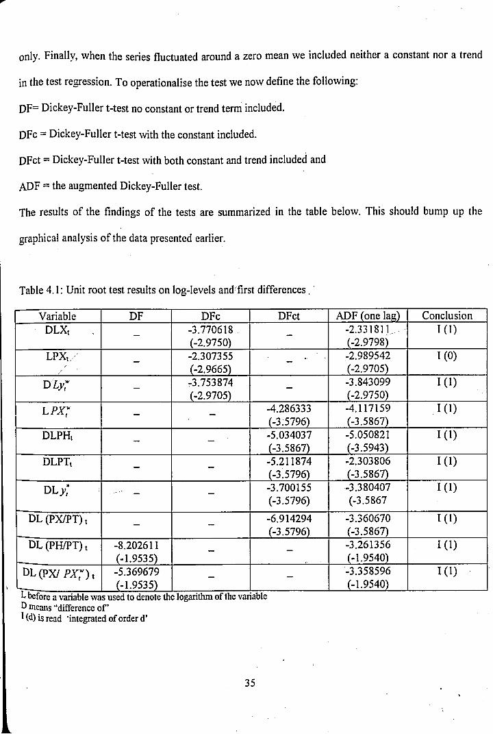
Table 4.1: Unit root test results on log-levels and first differences.
Variable DF DFc DFct ADF (one lag) ConclusionDLX,
--3.770618(-2.9750)
- -2.331811 (-2.9798)
H D
LPX,/-
-2.307355(-2.9665)
- " -2.989542(-2.9705)
1(0)
D Ly; --3.753874(-2.9705)
- -3.843099(-2.9750)
1 0 )
l p x ; - - -4.286333(-3.5796)
-4.117159(-3.5867)
I d )
DLPH, - —-5.034037(-3.5867)
-5.050821(-3.5943)
1(1)
DLPT,- —
-5.211874(-3.5796)
-2.303806(-3.5867)
1(1)
DL^* - - -3.700155(-3.5796)
-3.380407(-3.5867
1(1)
DL (PX/PT) t- —
-6.914294(-3.5796)
-3.360670(-3.5867)
1(1)
DL (PH/PT) t -8.202611(-1.9535)
— —-3.261356(-1.9540)
1(1)
DL(PX/ PX?) t -5.369679(-1.9535)
— - -3.358596(-1.9540)
1(1)
L before a variable w as used to denote the logarithm o f the variable D means “difference o f ’I (d) is read 'integrated o f order d ’
35
All but one of the variables are integrated of order one [I (1)]. We varied the lag length of the
ADF test and found out that an increase in the lag length (up to the fourth lag) did not change the
conclusions of the ADF test. Although we hinted that the series PH/PT and VXJPX" might be stationary
the tests above show otherwise. Perhaps, after all, the return of the graphs to a mean value (if any) was
not rapid enough. For the series that we had difficulties describing graphically we tested all the
regression specifications indicated in the table above.
4.3 Cointegration and ECM modelling
Formally, if a series yt~I (d) and xt~I (b) and the linear combination of the two, namely zt = yt-
kxt~I (d-b), then yt and xt are cointegrated of order (d-b). A test for cointegration would involve
performing unit root test on zt (the error term). If we reject stationarity of the linear combination, then
we can say that yt and xt are cointegrated. In this study we utilized the Engle and Granger (1987) two-
step procedure where; first, we estimate a regression between export supply (and demand) on each of
their regressors and upon obtaining the residuals, test the residuals for their order of integration.
Concluding stationarity for the residual implies that there is cointegration. The export demand and
supply theory is stated in levels and differencing the variables to render them stationary transforms
theory into a relationship of changes (resulting in loss of long run information about the variables).
However we can retain this long run information by the use of an error correction model.
36
4.4 Hypotheses of the study
The study will test will test the following hypotheses:
1. Kenya is a small country, that is, its manufactures export prices are equal to the
world price (PX" ) of manufactured goods.
2. An increase in income-abroad (external economic activity) lead to increased
demand for manufactured exports.
3. The relative increase of the domestic price of manufactured goods to the price in
the world markets decreases the quantities demanded of the manufactured goods.
4. Increases in the relative price of manufactured goods to the price of other
tradables increases the supply of the manufactures.
5. An increase in the real exchange rate variable (PH/PT) reduces the level of supply
of manufactured exports.
6. Increases in domestic capacity (y*) lead to increases in the supply of
manufactured goods.
J ‘
3 7
CHAPTER FIVE
PRESENTATION OF RESULTS AND INTERPRETATIONS
This chapter presents and discusses the empirical findings. The issue of the small country
assumption precedes the estimation of the structural estimates. For the structural estimates, use is made
of models A and B (see methodology). The diagnostic tests are reported for each regression. Similar test
statistics are given for each of the models. Before continuing it will be essential to expound on the test
statistics used.
t-statistics are conventionally calculated to determine whether individual coefficients arer
significantly different from zero. The null hypothesis (Ho), of a zero coefficient is rejected for large
values of t (that is, t values greater than or equal to a value of two). The standard error (std. Error) test
serves a similar purpose. A variable has a significant coefficient if that coefficient is greater than twice
its standard error. PartR2 gives the explanatory power of each variable holding the other variables
constant.
R2 measures the goodness of fit of the regression. The F- statistic tests the null hypothesis that all
the regression coefficients except the intercept are zero. In the case of the general overparameterized
model in appendix 4 table 1 the F- statistic with 14 and 13 degrees of freedom for the numerator and
denominator respectively is 13.949 and its probability value (of zero) is given in the square brackets
{that is, F (14, 13) = 13.949 [0.0000]}. The reported F-statistic in the tables for similar degrees of
freedom is 2.57 (at the 5% level). The calculated F is greater than the reported F and the null is rejected.
Generally ‘large’ values of F will mean rejection of the null hypothesis.
o is the residual standard deviation. It is the standard deviation of the difference between the actual
and fitted values in the regression. Smaller values of a are preferable. If movement from the
38
overparameterized model to the preferred model reduces the c statistic then this implies that there is no
loss of information in the exclusion process.
RSS is the residual sum of squares (RSS=ct2 (T-K). If say model 2 has a higher RSS than model 1,
then model 2 is nested in model 1.
AR tests for error autocorrelation (serial correlation) It is a Lagrange Multiplier (LM) test for
autocorrelation. In some instances both the F-test and Chi2 test are reported. The LM test is valid for
models with lagged dependent variables, whereas neither the Durbin-Watson (DW) nor the residual
correlogram provide a valid test in that case. The null hypothesis of no autocorrelation is rejected if the
test statistic is too high.
The normality test checks whether the variable at hand (the residual) is normally distributed. The
null hypothesis of normality is rejected at 5% if a test statistic greater than 5.99 is observed. In the case
below (and in subsequent cases) normality test statistic is a chi test. In the preferred model in table 5.1
below the chi test with two degrees of freedom is 2.0174 with a probability value of 0.3647 given in/
square brackets (that is, chi2 (2)=2.0174[0.3647]) and clearly normality is not rejected. The Regression
Specification Test (RESET) checks if y (t) depends on its squared values [i.e. yA(t)n where n=2,3,4...]
thus testing for functional form misspecification. The test statistics below is smaller than the reported
value and we conclude that model is specified correctly.
Heteroscedasticity tests if the error terms have constant variances. The null hypothesis of no
heteroscedasticity is rejected if the test statistic is too high.
In all the estimations we used the general-to-simple modelling strategy, which has the following general
steps:
1. It begins with the dynamic model formulation
2. We check for data coherence and cointegration
3 9
3. Unwanted regressors are deleted to obtain a parsimonious model and
4. The validity of the model is checked by use of standard tests. Schwarz Criterion (SC), Hannan-
Quinn Criterion (HQ), and c-values monitor progress.
5.1 The small country assumption
To test the small country assumption, the reduced form of model A, (the most general model) was
estimated. If the small country assumption can be rejected this is..evidence that the country faces a small
demand price elasticity.
5.1.1 The price equation
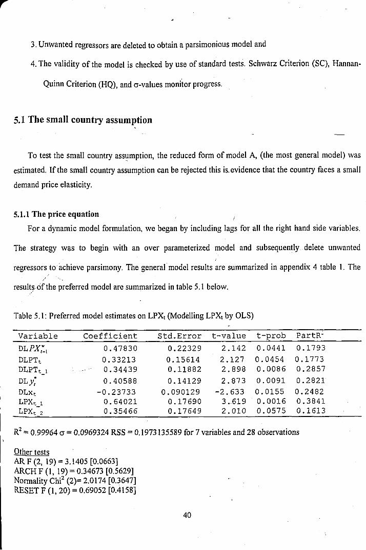
For a dynamic model formulation, we began by including lags for all the right hand side variables.
The strategy was to begin with an over parameterized model and subsequently delete unwanted
regressors to achieve parsimony. The general model results are summarized in appendix 4 table 1. The/
results of the preferred model are summarized in table 5.1 below.
Table 5.1: Preferred model estimates on LPXt (Modelling LPXt by OLS)
V a r i a b l e C o e f f i c i e n t S t d . E r r o r t-va l u e t-prob PartR'DL P X l x 0.47830 0.22329 2.142 0.0441 0.1793DLPTt 0.33213 0.15614 2.127 0.0454 0.1773DLPTt l — - 0.34439 0.11882 2.898 0.0086 0.2857D L y f* 0.40588 0.14129 2.873 0.0091 0.2821D L x t -0.23733 0.090129 -2.633 0.0155 0.2482L P X t l 0.64021 0.17690 3.619 0.0016 0.3841LPXt 2 0.35466 0.17649 2 .010 0.0575 0.1613
R2 = 0.99964 a = 0.0969324 RSS = 0.1973135589 for 7 variables and 28 observations
Other testsARF (2, 19) = 3.1405 [0.0663]ARCH F (1, 19) = 0.34673 [0.5629]Normality Chi2 (2)= 2.0174 [0.3647]RESET F (1, 20) = 0.69052 [0.4158]
4 0
There is no evidence of first or higher order autocorrelation in the equation errors, while other
statistics support the view that the distribution of the errors is identically and homoscedastically normal.
Nothing suggests that the price equation is mis-specified. Clearly the model captures the salient features
of the data and is consistent with the main implications of economic theory.
In our preferred price equation all the variables have the expected signs and are significant. If Kenya
is indeed a small country then the price for manufactured exports (PXt) should be given (that is,
dependent on the world price (PX”) alone}. We accordingly imposed zero restrictions on all the right
hand side variables aside PX” (which was restricted to a value of one) and tested the null hypothesis
that the coefficient terms of the variables are zero (that is, d22=d2i=d23=d24=d25=d26=0; d2i=l).
The reported Wald test (an F-statistic) for linear restrictions was F (7,21) = 817.18 [0.0000] **.
The null hypothesis tested (Ho) is that the restriction is binding. We conclude (because of the large F-
statistic) that the restriction is not binding. There is evidence that Kenya is not a small country in as far
as export of manufactured goods is concerned.
5.1.2 The quantity equation
The quantity equation was estimated following the same procedure. A look at the DLXt graph in
appendix 3 suggests that the series was disturbed by temporary shocks in the periods, 1981, 1983, 1998
and other minor shocks. Tests revealed that the other shocks were insignificant and were ignored to
avoid loss of degrees of freedom. Accordingly we introduced impulse dummies for the years 1981,1983
and 1998 (these are; il981, il983, and il998 respectively). The general model is given as table 2 in
appendix 4. Exclusion of the unwanted regressors (that is, those with low t-values and part R2) resulted
In the estimation of the preferred model whose results are summarized in table 5.2 below.
41
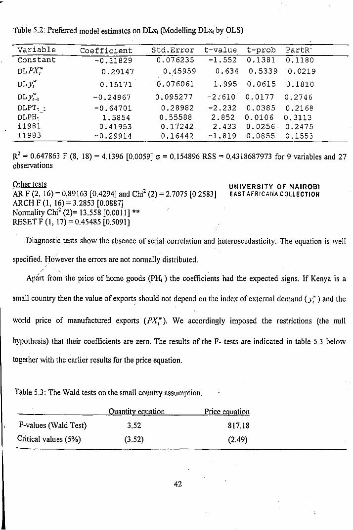
T ab le 5 .2: Preferred m o d e l estim ates o n D L x t (M o d ellin g D L x t b y O L S )
V a r i a b l e C o e f f i c i e n t S t d . E r r o r t-value t - p r o b P a r t R -C o n s t a n t - 0 . 11829 0.076235 -1.552 0.1381 0.1180d l p x ; 0.29147 0.45959 0.634 0 . 5 3 3 9 0.0219d l y ; 0.15171 0.076061 1.995 0 . 0 6 1 5 0.1810DL y l , -0.24867 0.095277 -2;610 0.0177 0.2746DLPTr 1 -0.64701 0.28982 -2.232 0 . 0 3 8 5 0.2168DLPHt 1.5854 0.55588 2.852 0 . 0 1 0 6 0.3113il981 0.41953 0 . 1 7 2 4 2 - 2.433 0 . 0 2 5 6 0.2475il983 -0.29914 0.16442 -1.819 0. 0 8 5 5 0.1553
R2 = 0.647863 F (8, 18) = 4.1396 [0.0059] a = 0.154896 RSS = 0.4318687973 for 9 variables and 27 observations
_U t n e rr ests U N I V E R S I T Y O F N A I R O B IAR F (2, 16) = 0.89163 [0.4294] and Chi2 (2) = 2.7075 [0.2583] EAST AFRICANA COLLECTION ARCH F (1, 16) = 3.2853 [0.0887]Normality Chi2 (2)= 13.558 [0.0011] **RESET F (1, 17) = 0.45485 [0.5091]
Diagnostic tests show the absence of serial correlation and heteroscedasticity. The equation is well
specified. However the errors are not normally distributed.s ' ■ ■/
Apart from the price of home goods (PHt ) the coefficients had the expected signs. If Kenya is a
small country then the value of exports should not depend on the index of external demand (>’," ) and the
world price of manufactured exports (PX*). We accordingly imposed the restrictions (the null
hypothesis) that their coefficients are zero. The results of the F- tests are indicated in table 5.3 belowi
together with the earlier results for the price equation.
Table 5.3: The Wald tests on the small country assumption.
_ ___________________ Quantity equation__________Price equation
F-values (Wald Test) 3.52 817.18
Critical values (5%) (3.52) (2.49)
4 2
The results of this tests show that the small country assumption could clearly be rejected, at the
conventional significance level of 5%. Kenya may thus have the market power in the manufactured
goods it exports and could use this advantage to gain market shares by offering a reduced price for these
goods. There is strong evidence of finite and relatively small demand price electricity. If the small
country assumption could not be rejected we could argue that Kenya faces a much larger, (possibly
infinite) demand price elasticity.
5.2 Structural estimates
5.2.1 Export demand estimates (model B)
Use was made of the estimated value for the manufactured exports (xt) derived from the equation of
the form, xt = f {(PX/PT) t-i, (PH/PT) t-i, yt-i, xt.i, (PX/PX") t-i}, that is xt on all the predetermined
/ A
variables b f the model. The generated xt ( x, ) was used to estimate the long run equilibrium relationship/
A
of the form, x, = f {(PX/PX") t.j, yt-i'v}. The preferred model had the form given below and the
overparameterized model is given in table 4 of appendix 4.
43
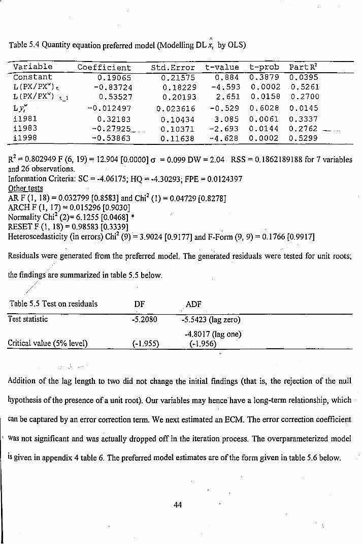
A
T able 5 .4 Q uantity eq u a tio n preferred m o d e l (M o d e llin g D L x , by O L S )
V a r i a b l e C o e f f i c i e n t S t d . E r r o r t - v a l u e t - p r o b Part R2^ C o n s t a n t 0.19065 0.21575 0.884 0 . 3 8 7 9 0.0395L (PX/PXW) t -0.83724 0.18229 -4.593 0 . 0 0 0 2 0.5261L (PX/PXW) t_i 0.53527 0.20193 2.651 0.0158 0.2700
- 0 . 012497 0 . 0 2 3 6 1 6 -0.529 0. 6 0 2 8 0.0145il981 0.32183 0.10434 3.085 0. 0 0 6 1 0.3337il983 - 0 . 2 7 9 2 5___ 0.10371 -2.693 0. 0 1 4 4 0.2762 ____il998 -0.53863 0.11638 -4.628 0 . 0 0 0 2 0.5299
R2 = 0.802949 F (6, 19) = 12.904 [0.0000] a = 0.099 DW = 2.04 RSS = 0.1862189188 for 7 variables and 26 observations.Information Criteria: SC = -4.06175; HQ = -4.30293; FPE = 0.0124397 Other testsAR F (1, 18) = 0.032799 [0.8583] and Chi2 (1) = 0.04729 [0.8278]ARCH F (1, 17) = 0.015296 [0.9030]Normality Chi2 (2)= 6.1255 [0.0468] *RESET F (1, 18) = 0.98583 [0.3339]Heteroscedasticity (in errors) Chi2 (9) = 3.9024 [0.9177] and F-Form (9, 9) = 0.1766 [0.9917]
Residuals were generated from the preferred model. The generated residuals were tested for unit roots;
the findings are summarized in table 5.5 below.
Table 5.5 Test on residuals DF ADF
Test statistic -5.2080 -5.5423 (lag zero)
-4.8017 (lag one)Critical value (5% level)___________(-1.955)_____ (-1.956)
Addition of the lag length to two did not change the initial findings (that is, the rejection of the null
hypothesis of the presence of a unit root). Our variables may hence have a long-term relationship, which
can be captured by an error correction term. We next estimated an ECM. The error correction coefficient
was not significant and was actually dropped off in the iteration process. The overparameterized model
•s given in appendix 4 table 6. The preferred model estimates are of the form given in table 5.6 below.
4 4
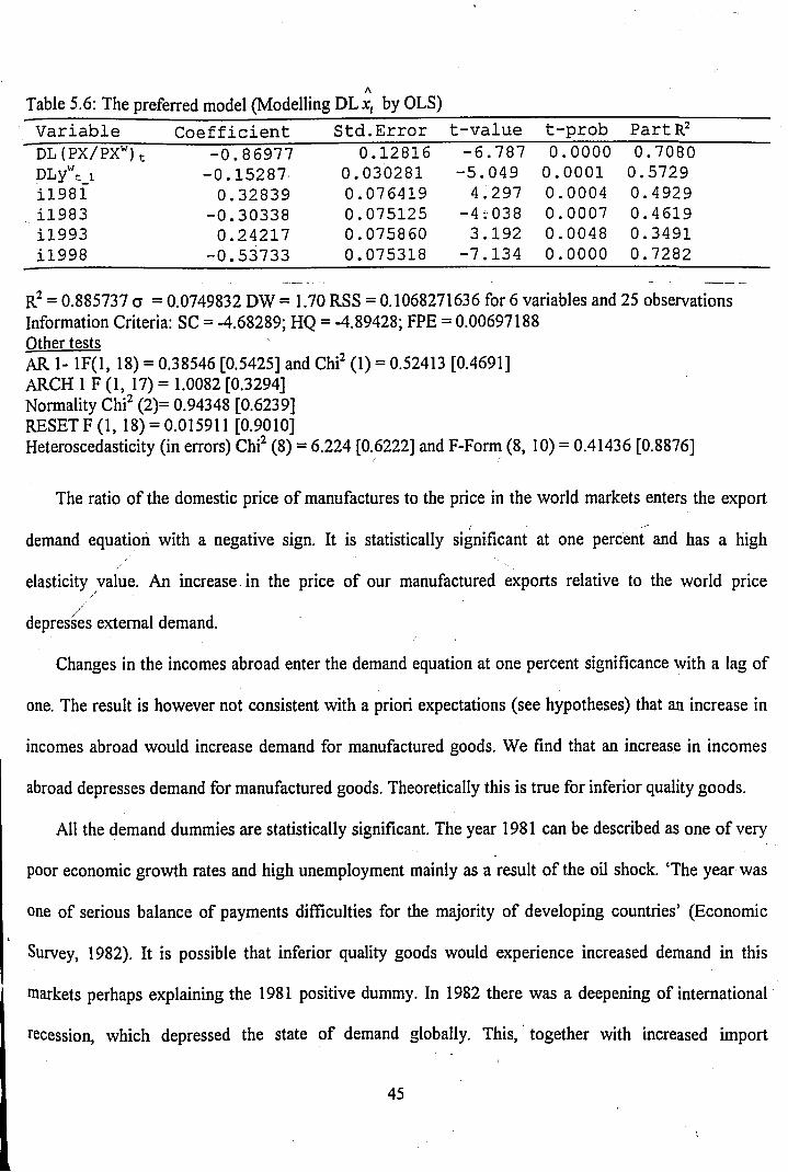
T ab le 5 .6: T h e preferred m o d e l (M o d e llin g D L x , b y O L S)
V a r i a b l e C o e f f i c i e n t S t d . E r r o r t-va l u e t - p r o b Part R2DL (PX/PXW) t - 0 . 8 6 9 7 7 0.12816 -6.787 0.0000 0.7080D L y wt i - 0 . 1 5 2 8 7 0.030281 -5.049 0.0001 0.5729il981 0.32839 0.076419 4.297 0.0004 0.4929il983 - 0 . 30338 0.075125 -4:038 0.0007 0.4619il993 0.24217 0.075860 3.192 0.0048 0.3491il998 - 0 . 5 3 7 3 3 0.075318 -7.134 0.0000 0.7282
R2 = 0.885737 ct = 0.0749832 DW = 1.70 RSS = 0.1068271636 for 6 variables and 25 observations Information Criteria: SC = -4.68289; HQ = -4.89428; FPE = 0.00697188 Other testsAR 1- 1F(1, 18) = 0.38546 [0.5425] and Chi2 (1) = 0.52413 [0.4691]ARCH 1 F (1, 17) = 1.0082 [0.3294]Normality Chi2 (2)= 0.94348 [0.6239]RESET F( l , 18) = 0.015911 [0.9010]Heteroscedasticity (in errors) Chi2 (8) = 6.224 [0.6222] and F-Form (8, 10) = 0.41436 [0.8876]
The ratio of the domestic price of manufactures to the price in the world markets enters the export
demand equation with a negative sign. It is statistically significant at one percent and has a high
elasticity value. An increase in the price of our manufactured exports relative to the world price
depresses external demand.
Changes in the incomes abroad enter the demand equation at one percent significance with a lag of
one. The result is however not consistent with a priori expectations (see hypotheses) that an increase in
incomes abroad would increase demand for manufactured goods. We find that an increase in incomes
abroad depresses demand for manufactured goods. Theoretically this is true for inferior quality goods.
All the demand dummies are statistically significant. The year 1981 can be described as one of very
poor economic growth rates and high unemployment mainly as a result of the oil shock. ‘The year was
one of serious balance of payments difficulties for the majority of developing countries’ (Economic
Survey, 1982). It is possible that inferior quality goods would experience increased demand in this
markets perhaps explaining the 1981 positive dummy. In 1982 there was a deepening of international
recession, which depressed the state of demand globally. This, together with increased import
45
restrictions of our main buyers (due to the debt problems in that time) could explain the negative 1983
impulse dummy. Financial market turbulence originating in Asia, the ban on fish exports to the
European Union and a reduction of the quota allocation for Kenyan garments (a major export) in 1998
could explain the negative 1998 impulse dummy.
In both models the error term is distributed as white noise. The Schwartz Criteria (SC) and a have
both declined implying no loss of information in moving from the general to the preferred model.
5.2.2 Export supply estimates (Model B)
Model B was represented by equations (9) and (10). In the first stage of the 2SLS we estimated an
equation of the form xt = f ((PX/PT) t-i, (PH/PT)t-i, yt-i, xt.i((PX/PXw)t.i,il981,il983,il998), that is xt on
all the predetermined variables of the model. The estimated coefficients were used to generate
/ A v A A
approximate values for manufactured exports (x ,) from the relation x, = xt - et. x, is thought to be less
A
correlated with the residuals, x, was used in the second stage and the results of the initial over
parameterized model indicated that there was evidence of the absence of heteroscedasticity and
autocorrelation. Furthermore, the errors were distributed normally (see table 5 in appendix 4).
All the variables are integrated of order one and cointegration is likely. A long run relationship of
the form xt = f ((PX/PT) t-i, (PH/PT) t-i, yt-i, Xt-i, (PX/PX") t-i), was estimated. So as to determine the
order of integration of the generated residuals DF and ADF tests were performed. If we cannot reject the
hypothesis that the et sequence is integrated of order zero then the variables may be cointegrated. The
v generated residual’s (et) unit root results are summarized in table 5.7 below.
4 6
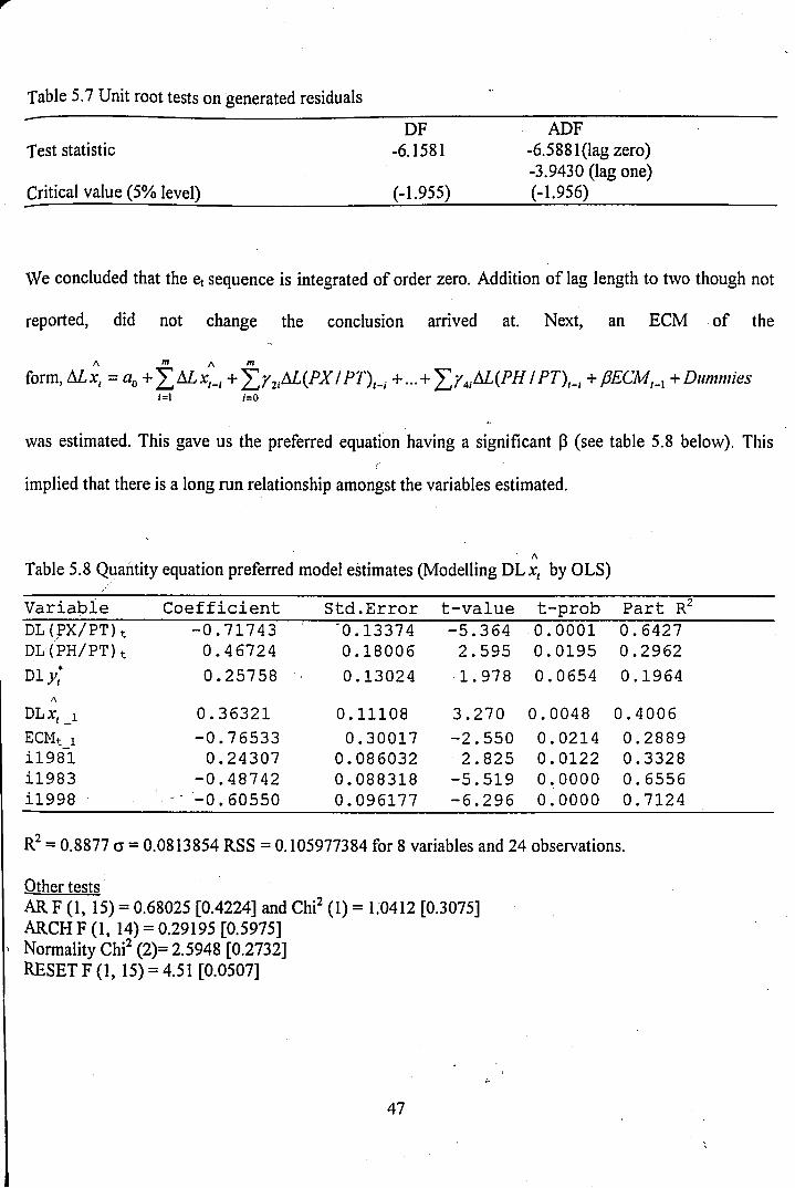
Table 5.7 Unit root tests on generated residuals
DF ADFTest statistic -6.1581 -6.5881 (lag zero)
-3.9430 (lag one)Critical value (5% level) (-1.955) (-1.956)
We concluded that the et sequence is integrated of order zero. Addition of lag length to two though not
reported, did not change the conclusion arrived at. Next, an ECM of the
A m A m _form, ALxt = a0 + '^A Lxl_j + ^ y 2iAL(PX I PT)t_j +... + ̂ Ty4jAL(PH / PT)t_t + f5ECMt_x + Dummies
i=l i=0
was estimated. This gave us the preferred equation having a significant P (see table 5.8 below). Thisr
implied that there is a long run relationship amongst the variables estimated.
A
Table 5.8 Quantity equation preferred model estimates (Modelling DLr, by OLS)
V a r i a b l e C o e f f i c i e n t S t d . E r r o r t-va l u e t- p r o b P art R 2DL(PX/PT)t - 0 . 7 1 7 4 3 '0.13374 -5.364 0 . 0 0 0 1 0.6427D L ( P H / P T ) t 0.46724 0.18006 2.595 0.0195 0.2962d i y t 0 . 2 5 7 5 8 • 0.13024 1.978 0.0654 0.1964
A
DL X, _1 0.36 3 2 1 0.11108 3.270 0.0048 0.4006E C M t i - 0 . 7 6 5 3 3 0.30017 -2.550 0.0214 0.2889i!981 0.24 3 0 7 0.086032 2 .825 0.0122 0.3328il983 - 0 . 4 8 7 4 2 0.088318 -5.519 0 . 0 0 0 0 0.6556i!998 ' - 0 . 6 0 5 5 0 0.096177 - 6 . 2 9 6 0 . 0 0 0 0 0.7124
R2 = 0.8877 a = 0.0813854 RSS = 0.105977384 for 8 variables and 24 observations.
Other testsAR F (1, 15) = 0.68025 [0.4224] and Chi2 (1) = 1.0412 [0.3075] ARCH F (1, 14) = 0.29195 [0.5975]Normality Chi2 (2)= 2.5948 [0.2732]RESET F( l , 15) = 4.51 [0.0507]
4 7
The ratio of the price of domestic exports to the price of other tradables has a large elasticity value
o f-0.72 and is statistically significant at one percent. A rise in the price of manufactured goods relative
to other tradables was expected a priori to increase supply.
The real exchange rate measure (PH/PT) is statistically significant at five percent and is positively
related to the level of supply of manufactured exports.
Capacity level enters the supply equation with a positive sign. A one percent rise in the level of
capacity would result in a 0.26 percent increase in manufactured export supply levels. At one place of
decimal, its coefficient is just significant at the ten percent level.
Changes in the first lag of past export levels positively influence current supply. This is indicated by
its elasticity estimate of 0.36, which is significant at the one percent level.
Despite the second oil shock of 1979/80 the 1981 impulse dummy indicates a positive impact on the
level of manufactured exports. It is possible that investors were responding to announcements of World
Bank supported reforms in the domestic economy in the early 1980s (WB, 1987).//The 1983 and 1998 impulse dummies are statistically significant at one and five percent levels
respectively. The negative 1983 impulse dummy could be explained by the failed coup attempt of
October 1982 that led to capital flight (RPED, 1993), and further there were major devaluations on the
exchange rate (prior to 1983), which may have reduced the dollar value of manufactured exports. The
only shocks witnessed after the 1993 reforms were in 1998. Events that are relevant to this period are
highlighted in the Economic Survey (1997). It is stated in part that ‘Inadequate rains, power rationing,
adverse effects of basic infrastructure constraints, rises in manufacturing processing costs attributed to
high prices of petroleum products and other key inputs, and prevailing high interest rates in 1996, led to
lower capacity utilization of manufacturing establishments in food processing, beverages, and tobacco
industries’. Furthermore, the year 1997 was an election year (election periods in Kenya are usually
4 8
marked by uncertainties that impact negatively on investment), there was also a ban on fish exports. All
these factors explain the negative and significant impulse dummy of 1998 and the general decline of the
dollar value of manufactured exports in subsequent periods.
The error correction term is significant at five percent. The coefficient of -0.77 for the ECM
suggests that seventy seven percent of the error from the previous year is corrected in the current year.
This is a high speed of adjustment.
Diagnostic tests show that there is absence of serial correlation as is indicated by the AR test and
absence of heteroscedasticity as indicated by the ARCH test. The normality test shows that the residuals
could still be approximated by a normal distribution. The model is well specified as the RESET test
indicates significance at ten percent.
5.2.3 Export supply estimates (Model A)
We have two endogenous variables (for model A). The two are price of manufactured exports (PXt)
and the quantity of manufactured exports (Xt) that is supplied or demanded.■ //W e estimated an equation of the form PXt = f (PXt.i'v,yt.iw,xt.j, PXt.j, (PX/PT)t.i,(PH/PT)t.i,yt.i) that is
price of manufactured goods on all the predetermined variables taking care to difference the variables
integrated of order one. We used the generated residuals to obtain an estimated value for the price of
A
manufactured goods using the relation PXt = PXt-et, where, et are the estimated residuals. PXt and
A
PX, are respectively the observed and estimated values for the price of manufactured goods.
The same procedure was applied to the quantity of manufactured exports (x t). For xt we estimated
the function of the form, x t = f ((PX/PT) t-i, (PH/PT) t-i, yt-i, xt. i, P X ^ , y"t yt.j w’ PXt-0, that is, xt on all
4 9
the predetermined variables in the model. To generate the estimated value of xt (x,) we used the relation
x, - Xt - et, where et are the generated residuals.
For both models the AR test indicated absence of serial correlation whereas the ARCH test
indicated lack of heteroscedasticity. The normality test showed that the residuals could still be
approximated by the normal distribution. Judging by the RESET test, the models were well specified.
Use was made of the value xt generated in the first stage of the 2SLS estimation. Table 3 in appendix
4 gives the results of the overparameterized model.
For the quantity equation all the variables of the preferred model were integrated of the first order
and accordingly we tested for the presence of cointegration. The steps of the process are given below.
We estimated the long run equilibrium relationship (i.e. without differencing) from which we
generated the residuals et. DF and ADF tests were performed on the et sequence in Pcgive. The results/
indicated that the et sequence was stationary in levels. Further, a plot of et revealed that it fluctuated//
around a zero mean. Table 5.9 below presents the results of the unit root tests.
U N I V E R S I T Y OF N A I R O B I EAST AFRICANA COLLECTION
Table 5.9 Unit root tests on generated residuals
________________________________________ DF______________ ADF__________Residual test statistic -2.4947 -2.4415
Critical value (at 5% level)________________(-1.954)__________ (-1.954)_________
We next estimated the error correction model (ECM) of the form:
' A m mX ,-,+ £ yvM y ^ +... + Yj yAiM(PH IPT),_,. +/1981+ /1983 + eu
i=l i=0 i=o
*5 0
Generally, if P=0 then there is no error correction and the variables do not have a long-term relationship.
Results indicated that the P coefficient was not statistically different from zero (it was actually dropped
off in the first iteration). The implication is that there is no stable long run relationship amongst the
variables. We proceeded to estimate xt equation in the first differences; table 5.10 below summarizes the
findings of the regression.
Table 5.10 Export quantity (xt) preferred estimates (Modelling DLxt by OLS)V a r i a b l e C o e f f i c i e n t S t d . E r r o r t - v a l u e t- p r o b Part R 2C o n s t a n t -0. 0 5 5 8 9 4 0.039163 -1.427 0.1716 0.1070DL(PX/PT)t - 0 . 98281 0.26539 -3.703 0.0018 0.4465DL(PX/PT)t i - 0 . 33173 0.21382 -1.551 0.1392 0.1240D L ( P H / P T ) t 0.65510 0.31872 2.055 0.0555 0.1990d i y, 0.50536 0.f27495 1.838 0.0836 0.1658D L x t 2 0.24278 0.18394 1.320 0.2044 0.0930il981 0.37554 0.17431 2.154 0.0458 0.2145il983 - 0 . 48043 0.16417 -2.926 0.0094 0.3350il998 - 0 . 45613 .0.15991 -2.852 0.0110 0.3237
R2 = 0.706924 F (8, 17) = 5.1257 [0.0023] a = 0.1454 DW = 2.02 RSS = 0.3594016743 for 9 variables and 26 observations
Other testsAR F (2, 15) = 0.46116 [0.6392] and Chi2 (2) = 1.5061 [0.4709] ARCH F (1, 15) = 0.2508 [0.6238]Normality Chi2 (2)= 4.0308 [0.1333]RESET F (1, 16) = 0.42964 [0.5215]
Diagnostic tests attest that the model is well-specified and other evidence point to the absence of
serial correlation and heteroscedasticity.
Changes in the relative price of manufactured exports to the price of other tradables negatively
influences change in manufactured export supply. It records a high elasticity value of -0.98, which is
statistically significant at the one percent level. Its first lag has the same sign but is insignificant.
51
The exchange rate measure (PH/PT) positively influences export supply at the ten percent
significance level with a one percent increase in the ratio (depreciation) resulting in a 0.66 percent
increase in export supply.
The capacity elasticity (coefficient of y*) and past export levels (second lag) have the appropriate
positive signs but are insignificant.
/
52
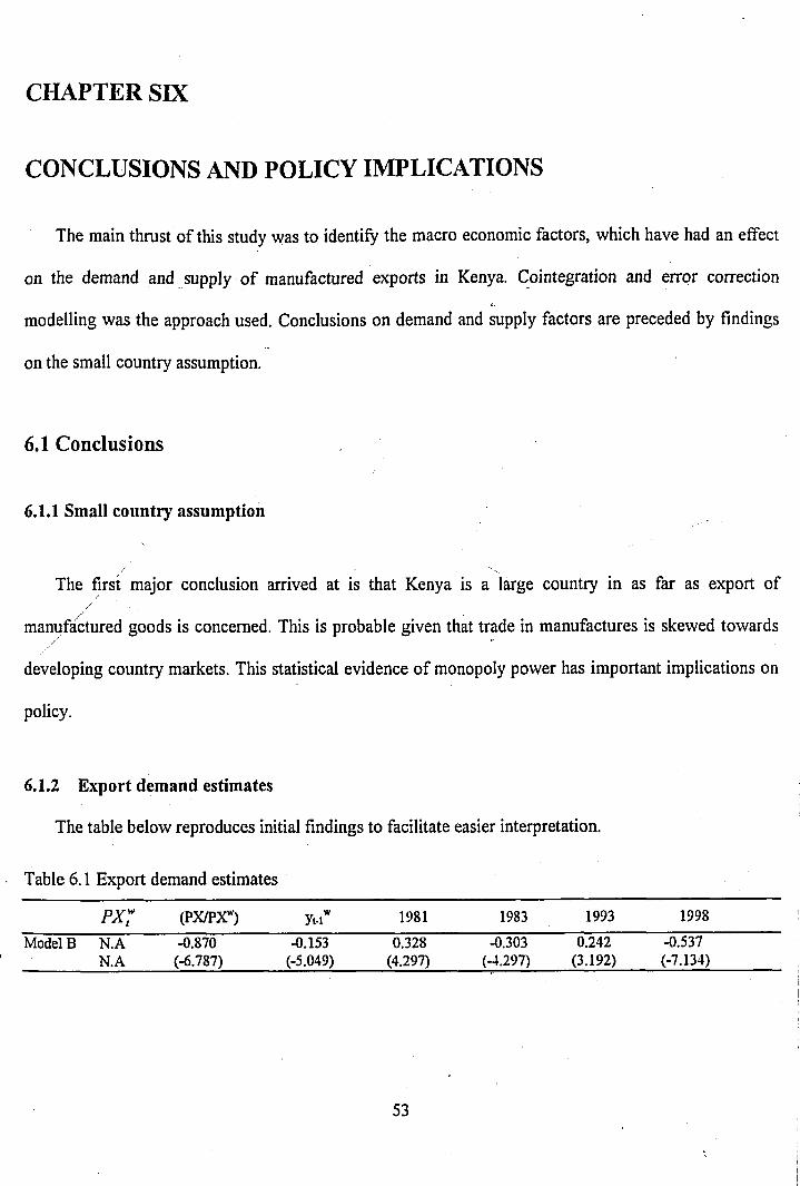
CHAPTER SIX
CONCLUSIONS AND POLICY IMPLICATIONS
The main thrust of this study was to identify the macro economic factors, which have had an effect
on the demand and supply of manufactured exports in Kenya. Cointegration and error correction
modelling was the approach used. Conclusions on demand and supply factors are preceded by findings
on the small country assumption.
6.1 Conclusionsr
6.1.1 Small country assumption
/The first major conclusion arrived at is that Kenya is a large country in as far as export of
manufactured goods is concerned. This is probable given that trade in manufactures is skewed towards
developing country markets. This statistical evidence of monopoly power has important implications on
policy.
6.1.2 Export demand estimates
The table below reproduces initial findings to facilitate easier interpretation.
Table 6.1 Export demand estimates
p x ; (PX/PX*) xr wy n 1981 1983 1993 1998
M odel B N .A -0.870 -0.153 0.328 -0.303 0.242 -0.537N .A (-6.787) (-5.049) (4.297) (-4.297) (3.192) (-7.134)
53
The income elasticity estimate (coefficient of y?) has an unexpected sign. We expected world
economic activity to positively influence export demand. The theoretical explanation we can seek
reassurance from is the argument that the demand for low quality goods declines as incomes improves.
Our manufactures may thus be inferior products.
The coefficient of the relative price of manufactured exports to the manufactured exports in the
world market (PX/PXW) has the appropriate sign and is highly significant. As was expected an increase
in the price of Kenya’s manufactured exports relative to the world price decreases the demand for our
manufactured goods. Kenya’s price elasticity of export demand is -0.87.
The insignificance of the error correction term (dropped off in the iterations) can be interpreted to
mean that our variables lack a stable long-run relationship.
The 1983 impulse dummy is negative perhaps reflecting the deepening of the world recession
in 1982 following the oil shock. Financial market turbulence and ban on fish exports to Europe explain/
the negative 1998 impulse dummy./
6.1.3 Export supply estimates
The table below summarizes the findings of the previous sections to facilitate easier interpretation.
Tables 6.2 Export supply estimates
(PX/PT), (P X /P D m (PH /PD t y ‘t X ,.i X t.2 ECMt-iModel A -0.983 -0.332 0.655 0.505 N .A 0.243 N .A
(-3.703) (-1.551) (2.055) (1.838) N .A (1.320) N .A
Model B -0.717 N .A 0.467 0.258 0.363 N .A -0.765(-5.364) N .A (2.595) (1.978) (3.270) N .A (-2.550)
We next interpret the findings of our preferred model; model B (B is preferred because the results
above indicate that Kenya is a large country).
54
The export supply price elasticity measure (PX/PT)t-i is -0.7. This can be interpreted as the long ,
price elasticity. The coefficient of (PX/PT) t is statistically significant at the one percent level. Mo]
(1988) reported short run price elasticity of manufactured export supply oscillating around 0.2. Bala.,
and others (1986) estimate price elasticities for Greece and the republic of Korea of between 1.5 and 2
If there is truth in the finding that Kenya is a large country (in as far as exports of manufactures to t
mainly regional markets is concerned) greater supply (ceteris paribus) can only be achieved at t.
expense of a reduced price. A rise in the price of exports depresses quantities demanded hence supply.
The real exchange rate elasticity (coefficient of (PH/PT) t} has a value of 0.47 and is statistics
significant at the five percent level. As expected an exchange rate depreciation (rise in PH/PT) increa;
the level of supply of manufactured goods.
The long run capacity elasticity (coefficient of y*) is statistically significant at the ten percent lev i
It is small, having a value of 0.26 - perhaps reflecting the reported low level of capacity utilizati(
(RPED, 1993). Its positive value implies that capacity level and exports of manufactured goods move///the same direction. The low level of capacity elasticity may mean that export levels may va
significantly without major changes in the former. The long run capacity elasticity fluctuated around 1
to 1.5 in Moran’s study, whereas the short run capacity elasticity varied between 0.1 and 0.4.
Past export levels (xt.i) have a positive influence on current supply. This is indicated by the positi\
long run elasticity estimate of 0.36, which is statistically significant.
The results of the preferred model show the ECM to be significant at five percent. The coefficient |
-0.76 for the ECM suggests that seventy six percent of the error from the previous year is corrected
the current year. This suggests a high speed of adjustment.
All the impulse dummies were significant. There is some indication that the announcement of tl
World Bank supported trade reforms in 1980 triggered a positive shock in 1981. This explains tl
i
55
positive and significant 1981 impulse dummy. The upward surge was however reverted in 1982 when
we had the failed coup attempt, which led to capital flight (RPED, 1993). The effects of the coup explain
the negative and significant 1983 impulse dummy. The only other significant shock was experienced in
1998. In 1996 and 1997 Kenya experienced several problems that impacted negatively on the supply
level of manufactured exports. The Economic Survey of 1997 lists ‘inadequate rains, power rationing,
adverse effects of basic infrastructure constraints, rises in manufacturing processing costs attributed to
high prices of petroleum products and other key inputs, and prevailing high interest rates in 1996’ as
factors that led to Tower capacity utilization of manufacturing establishments in food processing,
beverages and tobacco industries’. These factors are thought to be responsible for the decline in the
dollar value of manufactured exports after 1996. Further, this combination of factors may explain the
negative and significant 1998 impulse dummy.
The absence of a shock in 1993 despite major reforms is noteworthy. The absence of an expected
fillip may be explained by Foroutan’s observation that; between 1990-93 private and public investment
fell/ by fourteen and twenty three percent respectively. This was attributed to the stabilization
programme. The decline in real private investment may have rendered the reforms made in 1993 less
effective (Foroutan, 1998). Further the year 1993 recorded the highest inflation rate in Kenya (46%),
which could have wiped out the probable positive effects of the exchange rate depreciation.
Our export supply therefore has responded to: the ratio of manufactured exports prices to other
tradable goods prices (PX/PT)t , the real exchange rate, capacity output (y*), and past export levels (x t-
i). Apart from a short stint in the early 1980s, trade liberalization episodes have not been decisive in
influencing manufactured exports positively. It should however be noted that it took a long time (a
decade or so) before the Asian tigers reaped the benefits of trade liberalization.
5 6
■ The empirical results reviewed here indicate that prices clearly affect export demand and 5
Export supply is significantly influenced by domestic capacity and the real exchange rate, wi
increases in external economic activity suppress export demand.
57

6.2 Policy implications and recommendationsThe policy conclusions touch on the small country assumption, export demand and
export supply estimates.
6.2.1 The small country assumption
Empirically, we found Kenya to be a large country in as far as exports of
manufactured goods is concerned. Pricing policy becomes a vital tool in such a case.
Kenya can use this advantage to gain market shares by offering a reduced price for its
manufactured goods.
6.2.2 Export Demand
The foreign income elasticity (coefficient of y ”) is negative and this suggests that
our manufactures are inferior products. If its estimation is accurate, then the implication
is that Kenya cannot rely on external growth alone to generate adequate manufactured
export earnings. It can be argued that slow growth in our main trading partners should not
be an impediment to increased manufactured export revenues. Quality improvement (by
increasing competition) and encouragement of investment in export-oriented activities
are suggested policy options.
The large price elasticity measure (-0.87) of export demand (coefficient of PX/PXW)
indicates that pricing policy plays a key role in determining demanded quantities.
58
6.2.3 Export Supply
Real exchange rate devaluation/depreciation has been shown to be important for
exported quantities. It is therefore important that the variables that matter for exchange
rate determination must be properly managed. Edwards (1989) lists terms of trade, trade
liberalization, net capital inflows, government expenditure on non-tradables and
productivity growth in favour of tradables as important determinants of the real exchange
rate.
The domestic capacity (y *) matters for the supply of manufactured goods. Moran
(1988) argues that the proxy variable used captures a host of other factors that tend to
evolve slowly through time (such as the quality of the infrastructure). The importance of
domestic capacity therefore suggests that adjustment programmes designed to encourage
exports should promote domestic investment, improve the quality of infrastructure
(particularly in transport and communications), and provide other services essential for
exports.
Liberalization efforts in Kenya do not show a good report card yet; nonetheless, trade
liberalization measures have succeeded elsewhere (most notably in East Asia) in turning
agricultural based economies to exporters of chiefly manufactures. Although there have
been several starts at liberalization in Kenya (early 1980s and 1990s) the country is yet to
reap benefits. The impulse dummy for 1981 was positive and significant but it was
followed by a significant negative shock in 1983. The 1993 impulse dummy was
consistently insignificant in the export supply equations used. Shocks (e.g. the 1982 coup
and hostile macroeconomic environment prior to 1998) were significant in the export
supply equation. The significance of the negative shocks suggests that maintenance of an
59
environment devoid of political and macroeconomic instability would boost
manufactured exports supply. The ineffectiveness of reforms suggests that for reforms to
be successful other supply bottlenecks must be addressed concurrently.
The strong and lingering effect of past export levels on current supply further
emphasizes the importance of macro and political stability.
r
/
6 0
REFERENCES.
Amoko, Benn Lawrence 1996, “Determinants of the real exchange rate (RER) in Kenya. An empirical investigation: 1970 - 1995” M.A Research Thesis University of Nairobi 1996.
Balassa, Bela, Evangelosvoloudakis, Panagiotis Fylaktus, and Suk Tai Suh, 1986, “Export Incentives and Export Growth in Developing Countries: An Econometric Investigation.” World Bank Development Research Department Discussion Paper 159. Washington, D.C.
Behrman, J. 1976. Foreign Trade Regimes and Economic Development in Chile. New York: Columbia University Press.
Caballero, R. J. and Corbo, V. The Effect of Real Exchange Rate Uncertainty on Exports. The World Bank Economic Review, Vol. 3, No. 2, May 1989, p 263-278.
Coe, David T. and Alexander, W.H., 1998, “North-South Trade: Is Africa Unusual?” IMF Working Paper 00/45 Washington: International Monetary Fund.
Cuthbertson, K., Hall, S. G., Taylor, M. P. (1992) Applied Econometric Techniques. Hertfordshire:Harvester Wheatsheaf./
Edwards (1989), Real Exchange rates, Devaluation and Adjustment, MIT press//
Egwaikhide, F.O., 2000 Determinants o f Imports in Nigeria: A Dynamic Specification RP 91 AERC Nairobi.
Elbadawi, I. A. and Schmidt-Hebbel, K. (1996) ‘Macroeconomic Policies, Instability and Growth in the World’, paper presented at the AERC plenary of December 1996.
Foroutan, F., 1997 in Nash J. and Foroutan F. (cds)Trade Policy and Exchange Rate Reform in Sub Saharan Africa National Centre for Development Studies.
Glenday, G. and Ryan, T.C.I., (2000), ‘ Trade Liberalization and Growth in Kenya.’ EAGER policy paper No. 43
Havrylyshyn, O. (ed.), 1990,Exports o f Developing Countries: How Direction Affects Performance, A World Bank Symposium, Washington DC.
Helleiner, G.K. 1986. “Outward orientation, import instability and African economic growth: an empirical investigation.” In Sanjaya Lai and Frances Stewart (eds.) Theory and Reality in Development, Essays in Honour of Paul Streeten, Macmillan.,
61
Hemandez-Cata, E. 2000. “Raising Growth and Investment in Sub-Saharan Africa: What Can B Done?” In Masson, P., Gotur, P. and Lane, T. (eds) International Economic Policy Revie\ (Vol.2), IMF
International Monetary Fund, 1987, World Economic Outlook: Staff Studies - Expor Diversification in Developing Countries - Trends and the Impact of Policy, SM/87/93, 2 April.
Johsson, Gunnar, and Arvind Subramanian, 2000, “Dynamic Gains from Trade: Evidence froi South Africa.” IMF Working Paper 00/45 (Washington: Intwemational Monetary Fund).
Kaminski, B. and Ribound, M. (2000), Foreign Investment and Restructuring; The Evidence fron Hungary, World Bank Technical Paper, No.453, Europe and Central Asia Povert Reduction and Economic Management Series.
i/
Khadhuli, F.P.W. (1993), The Causes and Structures of Export Earnings Instability in Kenya; 196; - 1990 MA Thesis University of Nairobi.
Khan, M. and Knight, M. 1998. ‘Import Compensation and Export Performance in Developing , Countries. ’ Review of Economics and Statistics: May
Kimuyu, P.K. and S.K.Mugerwa, 1998Enterprice Response to Deficient Infrastructure. Discussior/ Paper No. 011/98. Institute of policy Analysis and Research.
Kimuyu, P.K. and Moyi, E., 1999. Revealed Comparative Advantage and Export Propensity ii. Kenya. Discussion Paper No. DP015/99. Institute of Policy Analysis and Research.
Lyakurwa, W.M., 1991, Trade policy and promotion in Sub-Saharan Africa, AERC, Nairobi
MacBean, A.I., \966fLxport Instability and Economic Development, Harvard University Press, Cambridge, Mass.
MacBean, A.I., I. Alasdair and D.I. Nguyena, 1980, ‘Commodity Concentration and Expon Instability: a Mathematical Analysis,’ The Economics Journal, vol. 90, pp 354 - 62.
Moran, C., 1988. A Structural Model for Developing Countries’ Manufactured Exports. The Worla Bank Economic Review, Vol.2, No.3 (September): 321-340.
Myint, H. (1958) ‘The classical Theory of International Trade and the Underdeveloped Countries,’ Economic Journal 68, pp. 317 - 337.
Mwega, F.M. (forthcoming), ‘Promotion of Non - Traditional Exports in Kenya, 1980 - 96’ In G.K. Helleiner, ed., Promotion o f Non - Traditional Exports in Sub - Saharan Africa.
6 2
Njuguna, S. Ndung’u (1999), Exchange rate policy in Kenya, AERC Research Paper No. 94 Nairobi.
Obote, A.M., 1981, First Steps to Recovery: Budget Speech 1981, Ministry of Planning and Economic Development.
Ochar, Willis (1999), The role of the exchange rate in the monetary approach to the Balance of Payments: Evidence from Kenya MA Thesis, department of economics, University of Nairobi, 1999.
Parades, C. E. 1987. ‘The Real Exchange Rate and the Performance of Manufactured Exports in Peru’ Department of Economics, Yale University, New Haren, Conn. Processed.
Pindyck, R.S. and Rubinfeld, D.L. (1991), Econometric Models and Economic Forecasts. New York: Me Graw - Hill Book Company.
Roberts, M.J. and Tybout J.R., 1997 ‘What Makes Exports Boom?’ Policy Research Working Paper. World Bank, Washington, D.C.
. U N I V E R S I T Y O F N A I R O B I^ „ . . . . EAST AFRICANA COLLECTION
Rudiger Dombusch (1992), ‘The Case for Trade Liberalization in Developing Countries’, Journalof Economic Perspectives, Vol.6, No.l, Winter: 69 - 85.
Sharpley, J. arid Lewis, S. R. (1988) ‘Kenya’s Industrialization, 1964-84’,Discussion Paper No. 242, Institute of Development Studies, Sussex.
Sodersten, B. and G.V. Reed, 1994. International Economics. London: Macmillan Press Ltd.//
Ssemogerere, G. and L.A. Kasekende, 1994, Constraints to the Development of Non - Traditional ex-ports in Uganda, 1981 -1990, AERC Nairobi
Syrquin, M. (1992) ‘Growth and Industrialization since 1965’, in G. K. Helleiner, Trade Policy and Industrialization in Turbulent Times, London: Routledge.
Thursby, Jerry, and Marie Thursby. 1984. ‘How Reliable Are Simple, Single Equation Specifications of Import Demand?’ Review of Economics and Statistics 66 (February): 120 - 28.
United Nations, Centre on Transnational Corporations, 1990 Vol. 1, Transnational Corporations and Economic Development; Vol.2.
United Nations, 1996. International Trade Statistics Yearbook, Vol. 1. New York
World Bank (1998) Annual world bank conference on development economics, World Bank, Washington D.C.
63
Word Bank (1987) Kenya: industrial Sector Policies for Investment and Export Growth, World Bank, Washington D.C.
_____ . (1996), World Development Report, World Bank, Washington, D.C.
________ . (1999), Global Economic Prospects and the Developing Countries, World Bank,Washington D.C.
. (2000a) Can Africa Claim the 21st Century? World Bank, Washington, D.C.
_________. (2000b) Energy Services for the Worlds Poor - Energy and Development Report 2000,World Bank, Washington D.C.
Yeats, A. J., Amjadi, A., Reincke, U., and Ng, F. 1999 ‘Did Domestic Policies Marginalize Africa in International Trade.’ Policy Research Working Paper. World Bank, Washington, D.C.
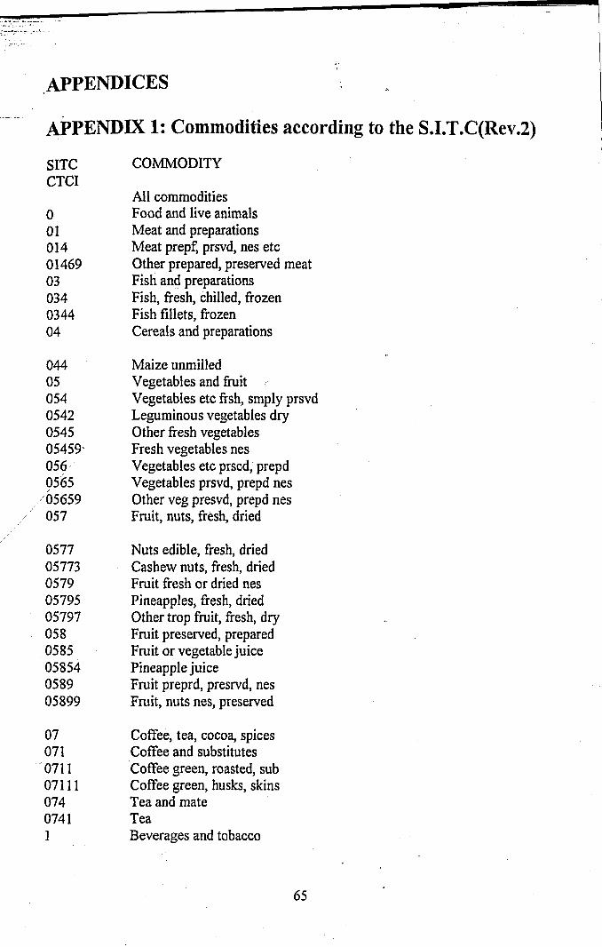
a p p e n d ic e s
APPENDIX 1: Commodities according to the S.I.T.C(Rev.2)
SITC COMMODITYCTCI
All commodities0 Food and live animals01 Meat and preparations014 Meat prepf, prsvd, nes etc01469 Other prepared, preserved meat03 Fish and preparations034 Fish, fresh, chilled, frozen0344 Fish fillets, frozen04 Cereals and preparations
044 Maize unmilled05 Vegetables and fruit054 Vegetables etc frsh, smply prsvd0542 Leguminous vegetables dry0545 Other fresh vegetables05459' Fresh vegetables nes056 Vegetables etc prscd, prepd0565 Vegetables prsvd, prepd nes
'05659 Other veg presvd, prepd nes057 Fruit, nuts, fresh, dried
0577 Nuts edible, fresh, dried05773 Cashew nuts, fresh, dried0579 Fruit fresh or dried nes05795 Pineapples, fresh, dried05797 Other trap fruit, fresh, dry058 Fruit preserved, prepared0585 Fruit or vegetable juice05854 Pineapple juice0589 Fruit preprd, presrvd, nes05899 Fruit, nuts nes, preserved
07 Coffee, tea, cocoa, spices071 Coffee and substitutes0711 Coffee green, roasted, sub07111 Coffee green, husks, skins074 Tea and mate0741 Tea1 Beverages and tobacco
65
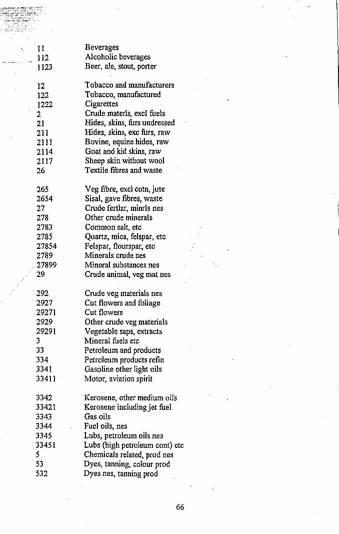
11 Beverages112 Alcoholic beverages1123 Beer, ale, stout, porter
12 Tobacco and manufacturers122 Tobacco, manufactured1222 Cigarettes2 Crude materls, excl fuels21 Hides, skins, furs undressed211 Hides, skins, exc furs, raw2111 Bovine, equine hides, raw2114 Goat and kid skins, raw2117 Sheep skin without wool26 Textile fibres and waste
265 Veg fibre, excl cotn, jute2654 Sisal, gave fibres, waste27 Crude fertlzr, minds nes278 Other crude minerals2783 Common salt, etc2785 Quartz, mica, felspar, etc27854 Felspar, flourspar, etc2789 Minerals crude nes27899 Mineral substances nes29 Crude animal, veg mat nes
292 Crude veg materials nes2927 Cut flowers and foliage29271 Cut flowers2929 Other crude veg materials29291 Vegetable saps, extracts3 Mineral fuels etc33 Petroleum and products334 Petroleum products refin3341 Gasoline other light oils33411 Motor, aviation spirit
3342 Kerosene, other medium oils33421 Kerosene including jet fuel3343 Gas oils3344 Fuel oils, nes3345 Lubs, petroleum oils nes33451 Lubs (high petroleum cont) etc5 Chemicals related, prod nes53 Dyes, tanning, colour prod532 Dyes nes, tanning prod
66
M*>
5322 Dye, tanning extracts, tanning
53221541541754171555515514553554 55415859 591 5911 66161146364 6426566 661 6612 67 674 69 691 6911 698 772
Vegetable tanning extracts, tannings Medicinal, pharm product Medicaments -containing antibiotics Perfume, cleaning etc prd Essential oils, perfume, etc Mixed perfume substances Perfumery, cosmetics, etc Soaps, cleansing etc preps SoapsPlastic materials etc Chemical materials nes Pesticides, disinfectants Insecticides, for retail Basic manufactures LeatherLeather bovine nes, equine Wood, cork manufactures nes Paper, paperboard and mfr Paper, etc, precut, arts of Textile yarn, fabrics, etc Non metal mineral mfs nes Cement etc building prod Cement Iron and steelIron, steel univ, plate, sheet Metal manufactures nes Structures and parts nes Structures, parts iron, steel Metal manufactures nes Machines, transport equipment Electrical machinery
729 Electrical machinery nes7291 Batteries, accumulators72991 Primary batteries, cells8 Miscellaneous manufactured goods89 Miscellaneous manufactured goods nes892 Printed matter893 Articles of plastic nes
Source: International Trade Statistics Year Book 1990.
6 7
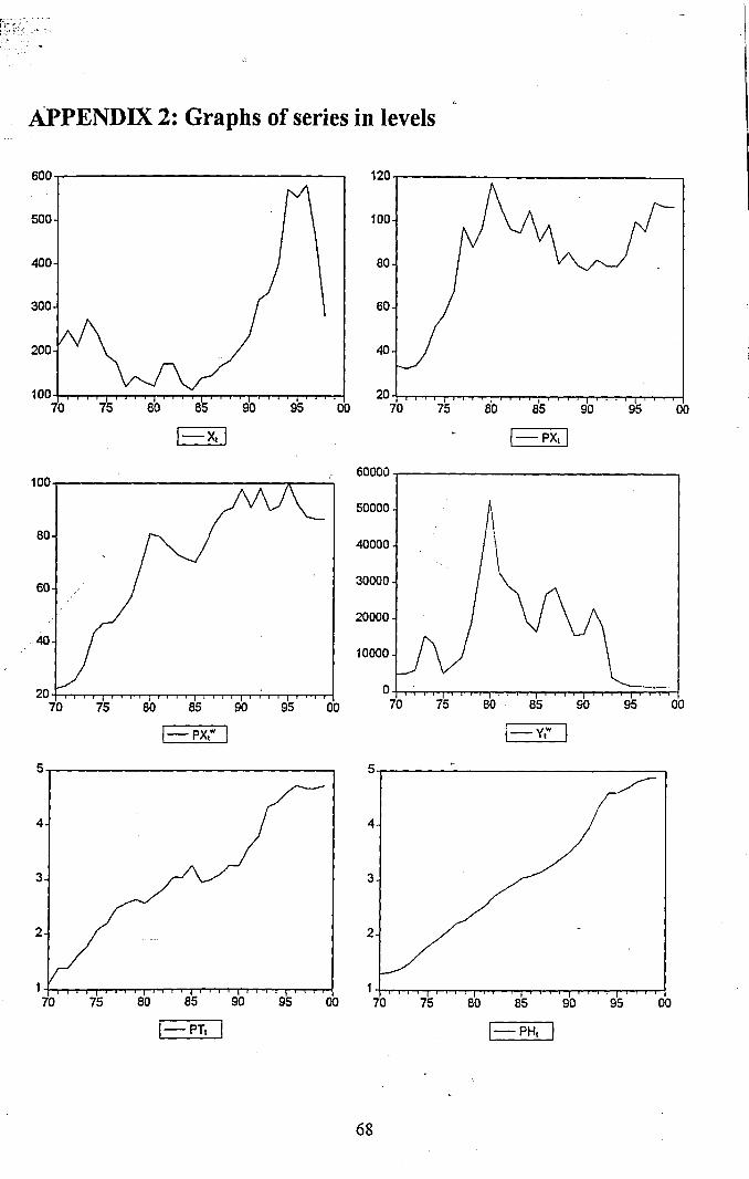
APPENDIX 2: Graphs of series in levels
6 8
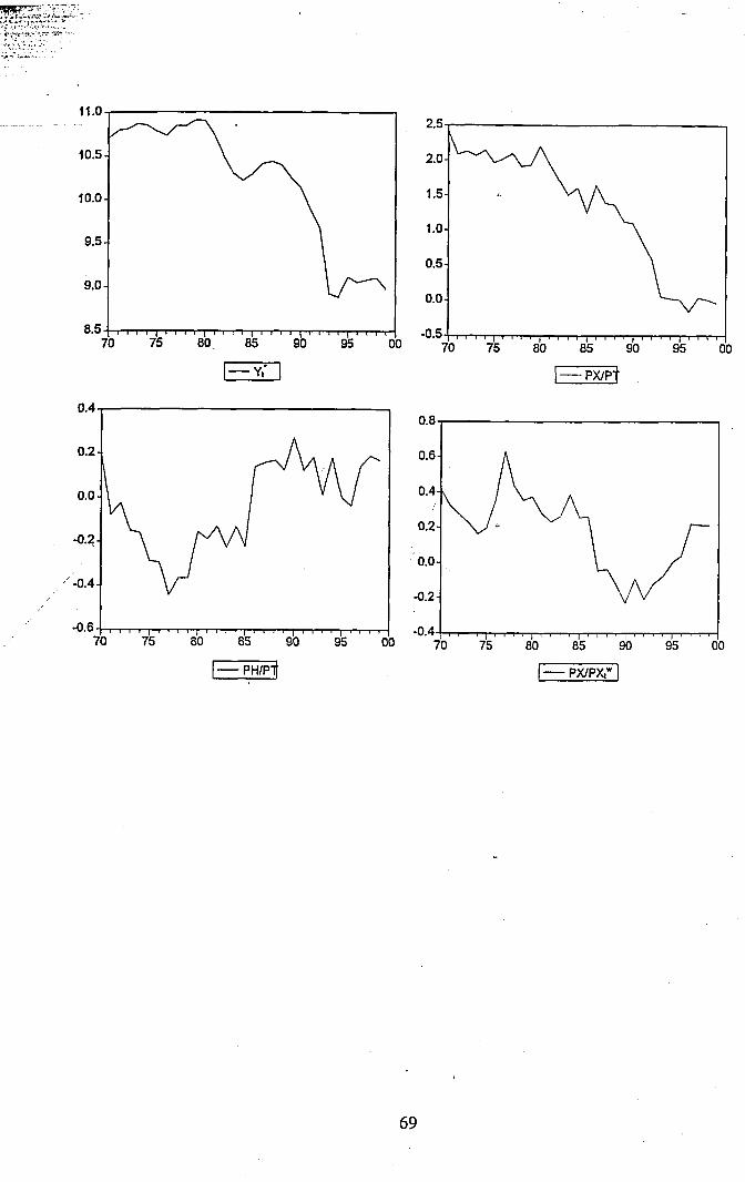
6 9
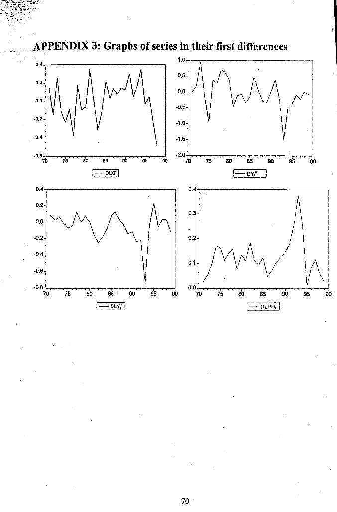
APPENDIX 3: Graphs of series in their first differences
----- DLY,' ----- DLPHi
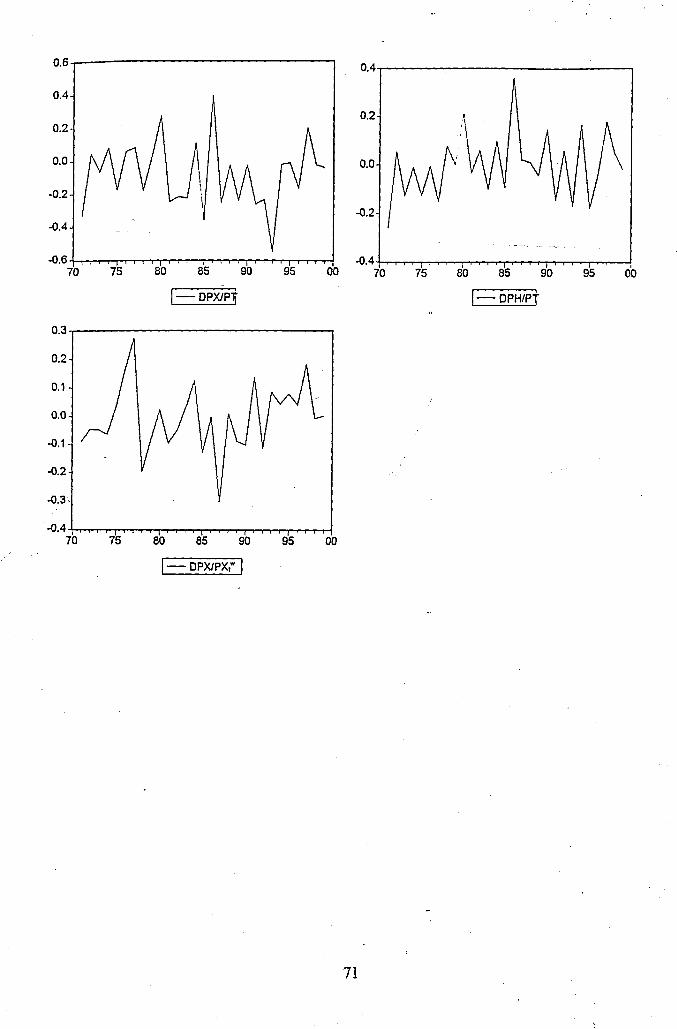
---- DPX/PX"
71
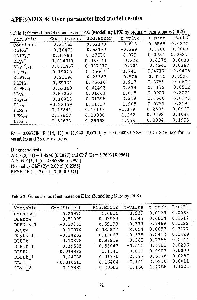
APPENDIX 4: Over parameterized model results
Table 1: General model estimates on LPXt [Modelling LPXt by ordinary least squares (OLS)]V a r i a b l e C o e f f i c i e n t Std. E r r o r t-value t - p r o b P a r t R 2C o n s t a n t 0.31465 0.52178 0.603 0 . 5 5 6 9 0.0272DL PXtw - 0 . 16472 0.55162 -0.299 0.7700 0.0068DL PX,r 0.36783 0.37570 0.979 0.3454 0.0687DLytw 0.014017 0 . 0 6 3 1 5 6 0.222 0.8278 0.0038DLy V i 0.061407 . 0 . 0 87270 0.704 0.4941 0.0367DLPTt- 0.19025 0.25667 0.741 O '. 4717 — Gr0405DLPTt--i 0.21194 0.23383 0.906 0.3812 0.0594DLPHt- 0.69334 0.75 6 1 6 0.917 0. 3 7 5 9 0.0607DLPHt-! 0.52360 0.62492 0.838 0.4172 0.0512DLyt 0.57055 0.31443 1.815 0.0 9 2 7 0.2021DLyt -i 0.10013 0.31395 0.319 0.7548 0.0078DLxt- - 0 . 22359 0.11737 -1.905 0.0791 0.2182DLXt--i - 0 . 16643 0.14111 -1.179 0.2593 0.0967LPX1--1 0.37858 0.30 0 0 6 1.262 0. 2 2 9 2 0.1091LPX.-a 0.52633 0.29663 1.774 0.0994 0.1950
R2 = 0.937584 F (14, 13) = 13.949 [0.0000] a = 0.108069 RSS = 0.1518270329 for 15 variables and 28 observations
Diagnostic testsARF (2, 11)= 1.4246 [0.2817] and Chi2 (2) = 5.7603 [0.0561] ARCH F (1, 11) = 0.067896 [0.7992]Normality Chi2 (2)= 2.8919 [0.2355]RESET F (1, 12) = 1.1728 [0.3001]
Table 2: General model estimates on DLxt (Modelling DLxt by OLS)
V a r i a b l e C o e f f i c i e n t S t d . E r r o r t-value t - p r o b P a r t R 2C o n s t a n t 0.25975 1.0856 0.239 0. 8 1 6 3 0.0063D L P X t w 0.51009 0.93963 0.543 0.6004 0.0317D L P X t w 1 -0.19703 0.59193 -0.333 0 . 7 4 6 9 0.0122D L y t w 0.17974 0 . 0 85822 2.094 0.0657 0.3277D L y t w 1 -0.10202 0.16067 -0.635 0. 5 4 1 2 0.0429D L P T t " 0.13375 0.36 9 1 9 0.362 0. 7 2 5 5 0.0144D L P T t 1 -0.19585 0.38043 -0.515 0. 6 1 9 1 0.0286D L P H t 0.014383 1.1541 0.012 0. 9 9 0 3 0.0000D L P H t 1 0.44735 0.91775 0.487 0 . 6 3 7 6 0.0257D L x t 1 -0.016613 0.16404 -0.101 0 . 9 2 1 6 0.0011D L x t 2 0.23882 0.20582 1.160 0.2758 0.1301
72
D Lyt - 0 . 23841 0.37047 -0.644 0. 5 3 5 9 ooD L y t _ l - 0 . 2 1 3 7 6 0.46 0 2 6 -0.464 0.6534 0 . 023<iLPXt - 0 . 8 7 0 7 6 0.37 0 2 0 -2.352 0.0432 0.3807L P X t 1 0.80701 0.30 7 7 0 2.623 0.0277 0.4332il983 -0.54718 0.21 2 5 0 - -2.575 0. 0 2 9 9 0.4242il981 0.35285 0.20374 1.732 0.1173 0.2500il998 -0.56944 0.18 1 6 5 -3.135 0. 0 1 2 0 0.5220
R2 = 0.83855 F (17, 9) = 2.7497 [0.0628] c = 0.148326 RSS = 0.1980063807 for 18 variables and 27 observations
Other testsAR F (1, 8) = 0.52327 [0.4901] and Chi2 (1) = 1.6576 [0.1979]ARCH F (1, 7) = 0.00013335 [0.9911]Normality Chi2 (2)= 0.30109 [0.8602] u n i v e r s i t y o p
RESET F (1, 8) = 0.39475 [0.5473] EASTAFRICANA COL lectio?
Table 3: The quantity equation general model (Modelling DLx, by OLS)V a r i a b l e C o e f f i c i e n t S t d . E r r o r t-value t - p r o b PartC o n s t a n t - 0 .073001 0 . 0 43433 - -1.681 0. 1 1 5 0 0.1679DL(PX/PT)r -1.0183 0.30308 -3.360 0.0047 0.4464DL (PX/PT) i -0.67815 0.41 8 8 0 -1.619 0.1277 0.1577DL(PH/PT)r 0.69385 0.32861 2.111 0.0532 0.2415D L ( P H / P T ) t i 0.53312 0.38042 1.401 0 . 1 8 2 9 0.1230D L y t 0.56678 0.29896 1.896 0.0788 0.2043D L y t i 0.060447 0.26937 0.224 0.8257 0.0036DL xt.) -0.21284 0 . 2 0 7 9 6 -1.023 0.3234 0.0696DL xt.2 0.27075 0.19178 1.412 0. 1 7 9 9 0.1246il981 0.36509 0.18770 1.945 0.0721 0.2127il983 -0.55807 0.17742 -3.145 0.0072 0.4141il998 -0.52288 0.17290 -3.024 0.0091 0.3951
R2= 0.745955 F (11, 14) = 3.7371 [0.0116] a = 0.149173 RSS = 0.3115382488 for 12 variables and 26 observations
Other testsAR F (2, 12) = 0.42724 and Chi2 (2) = 1.7283 [0.4214]] ARCHF (1, 12) = 0.021181 [0.8867]Normality Chi2 (2)= 2.2193 [0.3297]RESET F (1, 13) = 0.63366 [0.4403]
73
A
Table 4: Long run equilibrium relationship general model (Modelling DLx, by OLS)
V a r i a b l e C o e f f i c i e n t S t d . E r r o r t - v a l u e t-p r o b P a r t R2C o n s t a n t 0.13826 0.23 4 6 6 0.589 0.5635 0.0 2 0 0L (PX/PXW) t - 0 . 8 3 7 7 6 0.18454 -4.540 0.0003 0 . 5 4 8 0L (PX/PXW) t i 0.58699 0.20 5 0 9 " 2.862 0.0108 0.3252L y tw - 0 . 0 2 4 1 9 9 0 . 0 5 4 0 9 6 -0.447 0.6603 0 . 0 1 1 6Lywt i 0 . 0 15873 0 . 0 57785 0.275 0.7869 0.0044
. il981 0.30407 0.11355__ 2.678 0.0159 0.2967il983 - 0 . 2 8 2 3 9 0.10 5 0 6 -2.688 0.0156 0.2982il993 0.13209 0.12598 1.049 0.3091 0.0607il998 -0.-52 696 0.11766 -4.479 0.0003 0.5413
R2 = 0.824019 F (8, 17) = 9.9502 [0.0000] a = 0.0989077 DW = 2.30 RSS = 0.166306533 for 9 variables and 26 observations.Information Criteria: SC = -3.92422; HQ = -4.2343; FPE = 0.0131691
Other testsAR 1- 1F(1, 16) = 0.64063 [0.4352] and Chi2 (1) = 1.0009 [0.3171]] ARCH 1 F (1, 15) = 0.03449 [0.8552]Normality Chi2 (2)= 11.695 [0.0029] **RESET F (1, 16) = 0.91741 [0.3524]
Table 5: Quantity equation general model (Modelling DLx, by OLS)V a r i a b l e C o e f f i c i e n t S t d . E r r o r t-va l u e t - p r o b P a r t R 2C o n s t a n t - 0 . 0 9 1 9 3 9 0.025494 -3.606 0.0036 0.5201DL(PX/PT)t -1.0582 0.16621 -6.367 0 . 0 0 0 0 0.7716D L ( P X / P T ) t i - 0 . 5 3 4 4 9 0.22891 -2.335 0.0377 0.3124DL (PH/PT) t~ 0.55308 0.18846 2.935 0.0125 0.4179D L(PH/PT)t i - 0 . 0 8 7 8 6 8 0.23010 -0.382 0.7092 0.0120D L y t 0.23840 0.20544 1.160 0.2684 0. 1 0 0 9D L y t_i 0.20641 0.14910 1.384 0.1914 0.1377
A
DL X, . i 0.14788 0.13343 1.108 0.2895 0.0 9 2 9A
DLx, ,2 0.16198 0.10888 •• 1.488 0. 1 6 2 6 0.1557il981 0.42885 0.096482 4.445 0.0008 0.6221il983 - 0 . 50378 0 . 0 97122 -5.187 0.0002 0.6916il993 - 0 . 28181 0.14 2 9 5 -1.971 0.0722 0.2446
R2 = 0.90445 F (11, 12) = 10.326 [0.0002] a = 0.0787862 DW = 1.89 RSS = 0.07448711847 for 12 variables and 24 observations
74
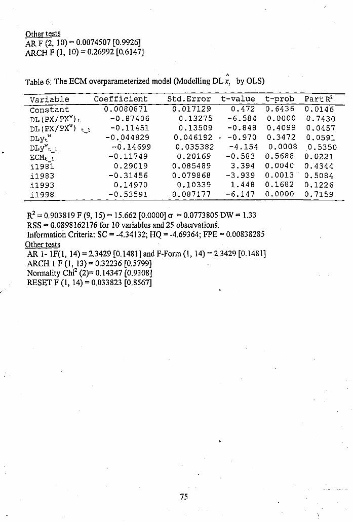
Other testsA R F (2, 10) = 0.0074507 [0.9926] ARCH F (1, 10) = 0.26992 [0.6147]
A
Table 6: The ECM overparameterized model (Modelling DL xt by OLS)
V a r i a b l e C o e f f i c i e n t S t d . E r r o r t - v a l u e t - p r o b Par t R2C o n s t a n t 0 . 0 0 8 0 8 7 1 0 . 0 1 7 1 2 9 0.472 0.6436 0.0 1 4 6DL (PX/PXW) t - 0 . 8 7 4 0 6 0.13275 -6.584 0.0000 0.7430DL (PX/PXW) t i - 0 . 1 1 4 5 1 0.13509 -0.848 0.4099 0.0457D L y tw - 0 . 0 4 4 8 2 9 0.046192 •• -0 . 9 7 0 0.3472 0.0591DL y wt i - 0 . 1 4 6 9 9 0 . 0 35382 -4.154 0.0008 0. 5 3 5 0E C M t i - 0 . 1 1 7 4 9 0.20 1 6 9 -0.583 0.5688 0.0221il981 0.29019 0 . 0 8 5 4 8 9 3.394 0.0040 0.4344il983 - 0 . 3 1 4 5 6 0.079868 -3.939 0.0013 0.5084il993 0.14970 0.10339 1.448 0.1682 0. 1 2 2 6il998 - 0 . 5 3 5 9 1 ,0.087177 -6.147 0.0000 0.7159
R2 = 0.903819 F (9, 15) = 15.662 [0.0000] cr = 0.0773805 DW =1.33 RSS = 0.0898162176 for 10 variables and 25 observations.Information Criteria: SC = -4.34132; HQ = -4.69364; FPE = 0.00838285 Other testsAR 1- 1F(1, 14) = 2.3429 [0.1481] and F-Form (1, 14) = 2.3429 [0.1481] ARCH 1 F (1, 13) = 0.32236 [0.5799]Normality Chi2 (2)= 0.14347 [0.9308]RESET F (1, 14) = 0.033823 [0.8567]
75
Top Related