


Languages
Pages
Legal

Advances in Sustainable Petroleum Engineering Science ISSN 1937-7991
Volume 2, Number 3 © 2011 Nova Science Publishers, Inc.
DEVELOPMENT OF NEW SCALING CRITERIA
FOR A FLUID FLOW MODEL WITH MEMORY
M. Enamul Hossain1
and M. Rafiqul Islam2
1Department of Petroleum Engineering
King Fahd University of Petroleum & Minerals (KFUPM)
Dhahran 31261, Saudi Arabia 2Department of Civil Engineering, Dalhousie University
Barrington Street, Halifax, NS, Canada, B3J-1Z1
ABSTRACT
New scaling criteria for an oil-water displacement process are presented in this
paper. The modified Darcy law with incorporating fluid memory is used to develop the
model equation. The mathematical model development of different scaling criteria for a
variety of scaling options is outlined here. Sets of similarity groups are derived by
inspectional and dimensional analysis for the displacement process using fluid memory
concept. To date there has been no rigorous presentation of the scaling requirements for a
displacement process where fluid memory has been counted. Relaxed sets of scaling
criteria based on major mechanisms of a process are determined. The purpose of this
paper is to present a method of developing a set of scaling criteria which permits different
relationships between saturation, capillary pressure, fluid pressure, and velocities
involving fluid memory in the model and prototype. The most efficient approach is
identified for oil-water displacement process when fluid memory has been taken care.
This new citation of idea can be used in enhanced oil recovery scheme where formation
and fluid properties are more complex in explaining their behavior.
Keywords: inspectional and dimensional analysis, displacement process, porous media,
prototype, model.
NOMENCLATURE
𝐴𝑦𝑧= cross sectional area of reservoir, 𝑓𝑡2
𝑓𝑜= ratio of oil phase velocity to total velocity, 𝑢𝑜𝑥 𝑈𝑥
𝑓𝑤= ratio of water phase velocity to total velocity, 𝑢𝑤𝑥 𝑈𝑥
Corresponding author: Email: [email protected]; [email protected]
M. Enamul Hossain and M. Rafiqul Islam 240
𝑔= gravitational acceleration, 𝑓𝑡 𝑠2
𝐻 = height of the formation, 𝑓𝑡
𝐽 𝑆 = dimensionless function
𝑘𝑜= reservoir permeability when fluid is oil, md
𝑘𝑤= reservoir permeability when fluid is water, md
𝐿= Length of the formation, 𝑓𝑡
𝑝= current reservoir pressure (at time t), psia
𝑝𝑐= capillary pressure of the reservoir, psia
𝑝𝑜= oil pressure, psia
𝑝𝑤= water pressure, psia
𝑝𝑖= initial reservoir pressure, psia
𝑆𝑜= oil saturation at p, dimensionless
𝑆𝑤= water saturation at p, dimensionless
𝑆𝑜𝑖= oil saturation at initial pressure pi, dimensionless
𝑆𝑤𝑖= water saturation at initial pressure pi, dimensionless
𝑡= time, hr
𝑢𝑜= reservoir oil velocity, 𝑓𝑡 𝑠
𝑢𝑤= reservoir water velocity, 𝑓𝑡 𝑠
𝑢𝑥= fluid velocity in porous media in the direction of x axis, 𝑓𝑡 𝑠
𝑈𝑥= algebraic summation of reservoir oil and water velocity in x-direction, 𝑓𝑡 𝑠
𝑢𝑤𝑥= reservoir water velocity in x-direction, 𝑓𝑡 𝑠
W= width of the formation, ft
𝑥= variable position from the wellbore along x-direction, 𝑓𝑡
𝑧= vertical distance from reservoir ground surface toward centre of the earth along z-direction, 𝑓𝑡
𝛼 = fractional order of differentiation, dimensionless
𝜉 = a dummy variable for time i.e. real part in the plane of the integral, s
𝜂= ratio of the pseudopermeability of the medium with memory to fluid viscosity, 𝑓𝑡3 𝑠1+𝛼 𝑙𝑏𝑚
𝜂𝑜= ratio of the pseudopermeability of the medium with memory to oil viscosity, 𝑓𝑡3 𝑠1+𝛼 𝑙𝑏𝑚
𝜂𝑤= ratio of the pseudopermeability of the medium with memory to water viscosity, 𝑓𝑡3 𝑠1+𝛼 𝑙𝑏𝑚
𝜌𝑜 = density of oil at pressure 𝑝, 𝑙𝑏𝑚 𝑓𝑡3
𝜌𝑤 = density of water at pressure 𝑝, 𝑙𝑏𝑚 𝑓𝑡3
𝜙 = porosity of the solid rock media, dimensionless
𝜃 = contact angle
𝜍 = interfacial tension, 𝑙𝑏𝑚 𝑠2
𝜇 = fluid dynamic viscosity, 𝑙𝑏𝑓𝑠 𝑓𝑡2
Γ= gamma function
Subscript
D = dimensionless quantity
R = reference quantity
o = oil
w = water
xo = oil in x-direction
yo = oil in y-direction
zo = oil in z-direction
Development of New Scaling Criteria for a Fluid Flow Model with Memory 241
xw = water in x-direction
yw = water in y-direction
zw = water in z-direction
INTRODUCTION
Laboratory experiments are the most useful way of developing predictive models for
various engineering applications. The usage of scaled laboratory models to simulate field
conditions such as petroleum reservoirs are known to be efficient in evaluating the advantages
of a recovery process (Coskuner and Bentsen, 1988). This procedure would be well accepted
when scaling laws would be known in order to scale up laboratory results to field conditions.
This scaling up offers a formidable challenge in scenarios involving complex solid-fluid,
fluid-fluid interactions, which are predominant in a displacement process, such as in enhanced
oil recovery (EOR) of petroleum engineering. In scaling such miscible displacements, an
inspectional analysis, complemented by dimensional analysis is utilized to obtain a set of
scaling criteria (Pozzi and Blackwell, 1963). A scaled model is designed on the basis of the
principle of similarity. Such a model is characterized by the same ratios of dimensions,
forces, velocities, and temperature. The model geometry, pressure drop, flow rate, time factor,
etc are different for different approaches depending on the type of scaling criteria used. Each
approach has its unique advantages and disadvantages (Bansal and Islam, 1994). Therefore,
the performance of any displacement process in porous media is governed by the related
variables. These variables can be combined by dimensionless groups.
It should be noted that the complete set of scaling criteria is very difficult to satisfy.
Therefore, some of the similarity groups must be relaxed in order to satisfy the most
important parameter of the specific reservoir activities. The choice of which requirements to
relax depends on the particular process being modeled. Scaling of the phenomena considered
to be least important to a particular process might be relaxed without significantly affecting
the major features of the process. The choice of an approach depends on the importance of the
phenomena that are not scaled by that approach. As an example, if one considers such an
approach where, model and prototype have the same morphology, the same fluids, and are
operated at the same conditions of pressure and temperature, the scaling groups such as
geometric factors, morphology factors, ratio of gravitational to viscous forces are completely
satisfied. The criteria used most widely for high pressure models are outlined by Pujol and
Boberg (1972). The high pressure models typically employ the same fluids in the model as
found in the prototype field (Kimber et al., 1988).
There are two basic available methods in the literature by which the dimensionless
groups can be obtained (Geertsma et al., 1956; Loomis and Crowell, 1964; Rojas, 1985;
Islam, 1987). The methods used are inspectional analysis and dimensional analysis. They
have discussed extensively the methods and their applications in the petroleum industry. The
researchers mainly focused their works on oil displacements and recovery processes (Pujol
and Boberg, 1972; Farouq Ali and Redford, 1977; Lozada and Farouq Ali, 1987; Lozada and
Farouq Ali, 1988; Kimber et al., 1988; Islam and Farouq Ali, 1990; Islam and Farouq Ali,
1992; Bansal and Islam, 1994; Islam et al., 1994; Sundaram and Islam, 1994). Basu and Islam
(2007) studied a scaling up of chemical injection experiments. They presented a series of
chemical adsorption tests and provide one with the scaled up versions. They gave a guideline

M. Enamul Hossain and M. Rafiqul Islam 242
how to interpret laboratory experimental results and apply the scaling laws to predict field
behavior. They also compared their findings with numerical simulation results. However,
Scaled physical models have been reported to be more desirable than numerical simulations
(Farouq Ali et al., 1987). This is largely applicable for recovery methods where phase
equilibrium and gravitational forces are significant factors.
Recently, Hossain et al. (2009a) studied the scaling criteria for designing waterjet drilling
laboratory experiments for reasonably simulating a given oilfield operation. They proposed a
scaling approach and derived the dimensionless groups for the waterjet drilling technique. A
scaled model is developed including a complete set of similarity groups where experimental
results are scaled up for field application. In addition, empirical models for the depth (D) and
rate of penetration (ROP) are established based on scaled-up process for a drilling oil field
application. However, there is no available literature or model that deals with the scaling
criteria and its applications based on displacement process with memory concept. The
objectives of this paper are to study the relevant variables engaged in displacement process
where the notion of memory is considered during the development of the model equation.
Finally dimensionless groups, relaxed sets of similarity groups and an efficient approach are
identified using inspectional and dimensional analysis. In future, the usage of prototypes are
proposed for proper selection of a subset of scaling groups that may adequately represent the
significant physical interactions dominant in the displacement process. The choice of the
subset should be applicable to dimensionless groups which may annul the effect of the
parameters and do not contribute adequately to the fluid-fluid displacement process.
MODEL DESCRIPTION
A reservoir surrounded with known geometry contains only oil and water. The flow is
parallel to all-axis (Figure 1). The pressure and saturation are uniform throughout the
reservoir. The pore space is assumed to be completely filled with oil and water.
Figure 1. Porous media considering its state.
Water is injected at one end maintaining a given constant filtration velocities 𝑢1𝑜 , 𝑢1𝑤 .
Just before the production starts up, the saturation and pressure of oil and water is known. The
injection well is in the center of the reservoir and production well surrounds the injection
well. The injection and production of water and oil is at a definite rate or pressure. The oil and
Development of New Scaling Criteria for a Fluid Flow Model with Memory 243
water components are assumed to be immiscible, therefore, there is no mass transfer between
the oil and water phase. In addition, there is no slippage in flow. Moreover, it is assumed that
there is no effect of capillary pressure and initially both fluids are incompressible and have
constant viscosities.
DERIVATION OF MATHEMATICAL MODEL
Let us consider the modified Darcy law with fluid memory for both oil and water phase
during the production. The equations of state for each fluid, relationship between the capillary
pressure and saturation have been presented as constitutive relationships and constrains in
Table 1. A model can be developed for displacement of oil by water in the porous media by
using the modified Darcy law (Hossain et al., 2007; Hossain et al., 2008; Hossain et al.,
2009b) with fluid memory which may be written as
𝑢𝑥 = − 𝜂 𝜕𝛼
𝜕𝑡𝛼 𝜕𝑝
𝜕𝑥 (1)
where, 𝜕𝛼
𝜕𝑡𝛼 𝜕𝑝
𝜕𝑥 =
𝑡− 𝜉 − 𝛼 𝜕2𝑝
𝜕𝜉 𝜕𝑥 𝑑𝜉
𝑡
0
Γ 1− α , with 0 ≤ 𝛼 < 1.
Table 1. Constitutive relationship and constraints
Constitutive relationship and constraints
1. 𝜌𝑜 = 𝜌𝑜 𝑝𝑜
2. 𝜌𝑤 = 𝜌𝑤 𝑝𝑤
3. 𝜂𝑜 = 𝜂𝑜 𝑘𝑜 , 𝜇𝑜 , 𝑝𝑜
4. 𝜂𝑤 = 𝜂𝑤 𝑘𝑤 , 𝜇𝑤 , 𝑝𝑤
5. 𝜙 ≅ constant
6. 𝑆𝑜 + 𝑆𝑤 = 1
7. 𝑝𝑜 − 𝑝𝑤 = 𝑝𝑐 𝑆𝑜 , 𝑆𝑤 ,𝜃𝑜 ,𝜃𝑤 ,𝜍, 𝑘
Equation (1) can be written as
𝑢𝑥 = − 𝜂 𝑡− 𝜉 − 𝛼
𝜕2𝑝
𝜕𝜉 𝜕𝑥 𝑑𝜉
𝑡
0
Γ 1− α (2)
Equation (2) can be written for oil and water as
𝑢𝑥𝑜 = − 𝜂𝑜
Γ 1− α 𝑡 − 𝜉 − 𝛼
𝜕2𝑝𝑜
𝜕𝜉 𝜕𝑥 𝑑𝜉
𝑡
0 (3)
𝑢𝑥𝑤 = − 𝜂𝑤
Γ 1− α 𝑡 − 𝜉 − 𝛼
𝜕2𝑝𝑤
𝜕𝜉 𝜕𝑥 𝑑𝜉
𝑡
0 (4)
M. Enamul Hossain and M. Rafiqul Islam 244
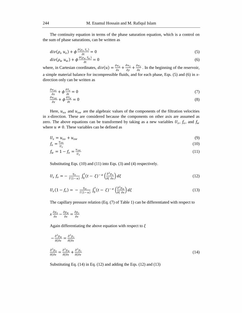
The continuity equation in terms of the phase saturation equation, which is a control on
the sum of phase saturations, can be written as
𝑑𝑖𝑣 𝜌𝑜 𝑢𝑜 + 𝜙𝜕 𝜌𝑜 𝑆𝑜
𝜕𝑡= 0 (5)
𝑑𝑖𝑣 𝜌𝑤 𝑢𝑤 + 𝜙𝜕 𝜌𝑤 𝑆𝑤
𝜕𝑡= 0 (6)
where, in Cartesian coordinates, 𝑑𝑖𝑣 𝑢 =𝜕𝑢𝑥
𝜕𝑥+
𝜕𝑢𝑦
𝜕𝑦+
𝜕𝑢𝑧
𝜕𝑧 . In the beginning of the reservoir,
a simple material balance for incompressible fluids, and for each phase, Eqs. (5) and (6) in x-
direction only can be written as
𝜕𝑢𝑥𝑜
𝜕𝑥+ 𝜙
𝜕𝑆𝑜
𝜕𝑡= 0 (7)
𝜕𝑢𝑥𝑤
𝜕𝑥+ 𝜙
𝜕𝑆𝑤
𝜕𝑡= 0 (8)
Here, 𝑢𝑥𝑜 and 𝑢𝑥𝑤 are the algebraic values of the components of the filtration velocities
in x-direction. These are considered because the components on other axis are assumed as
zero. The above equations can be transformed by taking as a new variables 𝑈𝑥 , 𝑓𝑜 , and 𝑓𝑤
where 𝑢 ≠ 0. These variables can be defined as
𝑈𝑥 = 𝑢𝑥𝑜 + 𝑢𝑥𝑤 (9)
𝑓𝑜 =𝑢𝑥𝑜
𝑈𝑥 (10)
𝑓𝑤 = 1 − 𝑓𝑜 =𝑢𝑥𝑤
𝑈𝑥 (11)
Substituting Eqs. (10) and (11) into Eqs. (3) and (4) respectively.
𝑈𝑥 𝑓𝑜 = − 𝜂𝑜
Γ 1− α 𝑡 − 𝜉 − 𝛼
𝜕2𝑝𝑜
𝜕𝜉 𝜕𝑥 𝑑𝜉
𝑡
0 (12)
𝑈𝑥 1 − 𝑓𝑜 = − 𝜂𝑤
Γ 1− α 𝑡 − 𝜉 − 𝛼
𝜕2𝑝𝑤
𝜕𝜉 𝜕𝑥 𝑑𝜉
𝑡
0 (13)
The capillary pressure relation (Eq. (7) of Table 1) can be differentiated with respect to
x 𝜕𝑝𝑜
𝜕𝑥−
𝜕𝑝𝑤
𝜕𝑥=
𝜕𝑝𝑐
𝜕𝑥
Again differentiating the above equation with respect to 𝜉
−𝜕2𝑝𝑤
𝜕𝜉𝜕𝑥=
𝜕2𝑝𝑐
𝜕𝜉𝜕𝑥
𝜕2𝑝𝑜
𝜕𝜉𝜕𝑥=
𝜕2𝑝𝑤
𝜕𝜉𝜕𝑥+
𝜕2𝑝𝑐
𝜕𝜉𝜕𝑥 (14)
Substituting Eq. (14) in Eq. (12) and adding the Eqs. (12) and (13)
Development of New Scaling Criteria for a Fluid Flow Model with Memory 245
𝑈𝑥 = − 𝜂𝑜
Γ 1 − α 𝑡 − 𝜉 − 𝛼
𝜕2𝑝𝑤𝜕𝜉𝜕𝑥
+𝜕2𝑝𝑐𝜕𝜉𝜕𝑥
𝑑𝜉
𝑡
0
− 𝜂𝑤
Γ 1 − α 𝑡 − 𝜉 − 𝛼
𝜕2𝑝𝑤𝜕𝜉𝜕𝑥
𝑑𝜉
𝑡
0
𝑈𝑥 = − 𝜂𝑜
Γ 1− α 𝑡 − 𝜉 − 𝛼
𝜕2𝑝𝑐
𝜕𝜉𝜕𝑥 𝑑𝜉
𝑡
0−
𝜂𝑜+ 𝜂𝑤
Γ 1− α 𝑡 − 𝜉 − 𝛼
𝜕2𝑝𝑤
𝜕𝜉𝜕𝑥 𝑑𝜉
𝑡
0 (15)
Substituting Eq. (11) in Eq. (8)
𝜕
𝜕𝑥 1 − 𝑓𝑜 𝑈𝑥 + 𝜙
𝜕𝑆𝑤
𝜕𝑡= 0
1 − 𝑓𝑜 𝜕𝑈𝑥
𝜕𝑥+ 𝑈𝑥 1 − 𝑓𝑜
𝜕 1−𝑓𝑜
𝜕𝑥+ 𝜙
𝜕𝑆𝑤
𝜕𝑡= 0
Since, 𝜕𝑈𝑥
𝜕𝑥= 0, the above equation becomes
−𝑈𝑥 1 − 𝑓𝑜 𝜕𝑓𝑜
𝜕𝑥+ 𝜙
𝜕𝑆𝑤
𝜕𝑡= 0 (16)
Substituting Eq. (15) in Eq. (16)
− − 𝜂𝑜
Γ 1− α 𝑡 − 𝜉 − 𝛼
𝜕2𝑝𝑐
𝜕𝜉𝜕𝑥 𝑑𝜉
𝑡
0−
𝜂𝑜+ 𝜂𝑤
Γ 1− α 𝑡 − 𝜉 − 𝛼
𝜕2𝑝𝑤
𝜕𝜉𝜕𝑥 𝑑𝜉
𝑡
0 1 − 𝑓𝑜
𝜕𝑓𝑜
𝜕𝑥+ 𝜙
𝜕𝑆𝑤
𝜕𝑡= 0
𝜂𝑜
Γ 1− α 𝑡 − 𝜉 − 𝛼
𝜕
𝜕𝜉 𝜕𝑝𝑐
𝜕𝑆𝑤
𝜕𝑆𝑤
𝜕𝑥 𝑑𝜉
𝑡
0+
𝜂𝑜+ 𝜂𝑤
Γ 1− α 𝑡 − 𝜉 − 𝛼
𝜕2𝑝𝑤
𝜕𝜉𝜕𝑥 𝑑𝜉
𝑡
0 1 − 𝑓𝑜
𝜕𝑓𝑜
𝜕𝑥+ 𝜙
𝜕𝑆𝑤
𝜕𝑡= 0
(17)
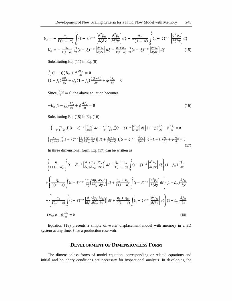
In three dimensional form, Eq. (17) can be written as
𝜂𝑜
Γ 1 − α 𝑡 − 𝜉 − 𝛼
𝜕
𝜕𝜉 𝜕𝑝𝑐𝜕𝑆𝑤
𝜕𝑆𝑤𝜕𝑥
𝑑𝜉
𝑡
0
+ 𝜂𝑜 + 𝜂𝑤Γ 1 − α
𝑡 − 𝜉 − 𝛼 𝜕2𝑝𝑤𝜕𝜉𝜕𝑥
𝑑𝜉
𝑡
0
1 − 𝑓𝑜𝑥 𝜕𝑓𝑜𝑥𝜕𝑥
+ 𝜂𝑜
Γ 1 − α 𝑡 − 𝜉 − 𝛼
𝜕
𝜕𝜉 𝜕𝑝𝑐𝜕𝑆𝑤
𝜕𝑆𝑤𝜕𝑦
𝑑𝜉
𝑡
0
+ 𝜂𝑜 + 𝜂𝑤Γ 1 − α
𝑡 − 𝜉 − 𝛼 𝜕2𝑝𝑤𝜕𝜉𝜕𝑦
𝑑𝜉
𝑡
0
1 − 𝑓𝑜𝑦 𝜕𝑓𝑜𝑦
𝜕𝑦
+ 𝜂𝑜
Γ 1 − α 𝑡 − 𝜉 − 𝛼
𝜕
𝜕𝜉 𝜕𝑝𝑐𝜕𝑆𝑤
𝜕𝑆𝑤𝜕𝑧
𝑑𝜉
𝑡
0
+ 𝜂𝑜 + 𝜂𝑤Γ 1 − α
𝑡 − 𝜉 − 𝛼 𝜕2𝑝𝑤𝜕𝜉𝜕𝑧
𝑑𝜉
𝑡
0
1 − 𝑓𝑜𝑧 𝜕𝑓𝑜𝑧𝜕𝑧
+𝜌𝑜𝑔 𝑧 + 𝜙𝜕𝑆𝑤
𝜕𝑡= 0 (18)
Equation (18) presents a simple oil-water displacement model with memory in a 3D
system at any time, 𝑡 for a production reservoir.
DEVELOPMENT OF DIMENSIONLESS FORM
The dimensionless forms of model equation, corresponding or related equations and
initial and boundary conditions are necessary for inspectional analysis. In developing the
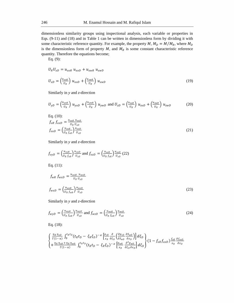
M. Enamul Hossain and M. Rafiqul Islam 246
dimensionless similarity groups using inspectional analysis, each variable or properties in
Eqs. (9-11) and (18) and in Table 1 can be written in dimensionless form by dividing it with
some characteristic reference quantity. For example, the property 𝑀, 𝑀𝐷 = 𝑀 𝑀𝑅 , where 𝑀𝐷
is the dimensionless form of property 𝑀, and 𝑀𝑅 is some constant characteristic reference
quantity. Therefore the equations become;
Eq. (9):
𝑈𝑅𝑈𝑥𝐷 = 𝑢𝑥𝑜𝑅 𝑢𝑥𝑜𝐷 + 𝑢𝑥𝑤𝑅 𝑢𝑥𝑤𝐷
𝑈𝑥𝐷 = 𝑢𝑥𝑜𝑅
𝑈𝑅 𝑢𝑥𝑜𝐷 +
𝑢𝑥𝑤𝑅
𝑈𝑅 𝑢𝑥𝑤𝐷 (19)
Similarly in y and z-direction
𝑈𝑦𝐷 = 𝑢𝑦𝑜𝑅
𝑈𝑅 𝑢𝑦𝑜𝐷 +
𝑢𝑦𝑤𝑅
𝑈𝑅 𝑢𝑦𝑤𝐷 and 𝑈𝑧𝐷 =
𝑢𝑧𝑜𝑅
𝑈𝑅 𝑢𝑧𝑜𝐷 +
𝑢𝑧𝑤𝑅
𝑈𝑅 𝑢𝑧𝑤𝐷 (20)
Eq. (10):
𝑓𝑜𝑅 𝑓𝑜𝑥𝐷 =𝑢𝑜𝑥𝑅 𝑢𝑜𝑥𝐷
𝑈𝑅 𝑈𝑥𝐷
𝑓𝑜𝑥𝐷 = 𝑢𝑜𝑥𝑅
𝑈𝑅 𝑓𝑜𝑅 𝑢𝑜𝑥𝐷
𝑈𝑥𝐷 (21)
Similarly in y and z-direction
𝑓𝑜𝑦𝐷 = 𝑢𝑜𝑦𝑅
𝑈𝑅 𝑓𝑜𝑅 𝑢𝑜𝑦𝐷
𝑈𝑥𝐷 and 𝑓𝑜𝑧𝐷 =
𝑢𝑜𝑧𝑅
𝑈𝑅 𝑓𝑜𝑅 𝑢𝑜𝑧𝐷
𝑈𝑥𝐷 (22)
Eq. (11):
𝑓𝑤𝑅 𝑓𝑤𝑥𝐷 =𝑢𝑤𝑥𝑅 𝑢𝑤𝑥𝐷
𝑈𝑅 𝑈𝑥𝐷
𝑓𝑤𝑥𝐷 = 𝑢𝑤𝑥𝑅
𝑈𝑅 𝑓𝑤𝑅 𝑢𝑤𝑥𝐷
𝑈𝑥𝐷 (23)
Similarly in y and z-direction
𝑓𝑤𝑦𝐷 = 𝑢𝑤𝑦𝑅
𝑈𝑅 𝑓𝑤𝑅 𝑢𝑤𝑦𝐷
𝑈𝑥𝐷 and 𝑓𝑤𝑧𝐷 =
𝑢𝑤𝑧𝑅
𝑈𝑅 𝑓𝑤𝑅 𝑢𝑤𝑧𝐷
𝑈𝑥𝐷 (24)
Eq. (18):
𝜂𝑅 𝜂𝑜𝐷
Γ 1− α 𝑡𝑅𝑡𝐷 − 𝜉𝑅𝜉𝐷
− 𝛼 𝑝𝑐𝑅
𝑥𝑅
𝜕
𝜕𝜉𝐷 𝜕𝑝𝑐𝐷
𝜕𝑆𝑤𝐷
𝜕𝑆𝑤𝐷
𝜕𝑥𝐷 𝑑𝜉𝐷
𝑡𝑅𝑡𝐷0
+𝜂𝑅 𝜂𝑜𝐷 + 𝜂𝑅 𝜂𝑤𝐷
Γ 1− α 𝑡𝑅𝑡𝐷 − 𝜉𝑅𝜉𝐷
− 𝛼 𝑝𝑤𝑅
𝑥𝑅 𝜕2𝑝𝑤𝐷
𝜕𝜉𝐷𝜕𝑥𝐷 𝑑𝜉𝐷
𝑡𝑅𝑡𝐷0
1 − 𝑓𝑜𝑅𝑓𝑜𝑥𝐷 𝑓𝑜𝑅
𝑥𝑅
𝜕𝑓𝑜𝑥𝐷
𝜕𝑥𝐷
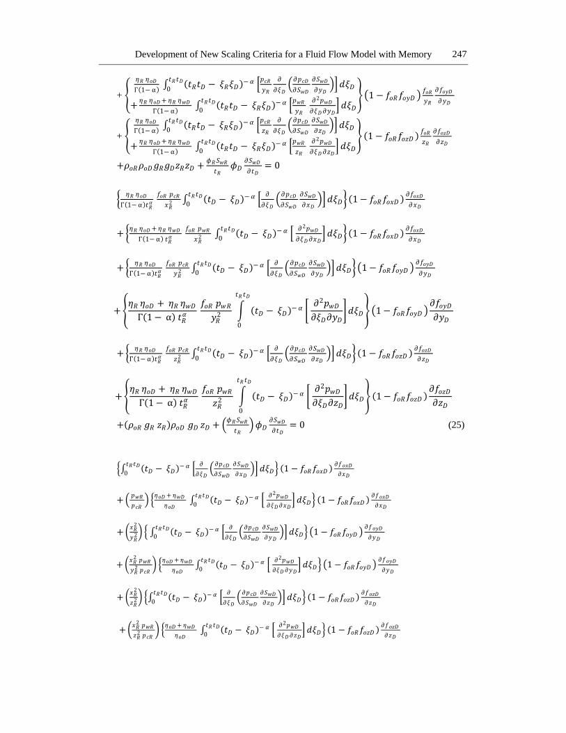
Development of New Scaling Criteria for a Fluid Flow Model with Memory 247
+ 𝜂𝑅 𝜂𝑜𝐷
Γ 1− α 𝑡𝑅𝑡𝐷 − 𝜉𝑅𝜉𝐷
− 𝛼 𝑝𝑐𝑅
𝑦𝑅
𝜕
𝜕𝜉𝐷 𝜕𝑝𝑐𝐷
𝜕𝑆𝑤𝐷
𝜕𝑆𝑤𝐷
𝜕𝑦𝐷 𝑑𝜉𝐷
𝑡𝑅𝑡𝐷0
+𝜂𝑅 𝜂𝑜𝐷 + 𝜂𝑅 𝜂𝑤𝐷
Γ 1− α 𝑡𝑅𝑡𝐷 − 𝜉𝑅𝜉𝐷
− 𝛼 𝑝𝑤𝑅
𝑦𝑅 𝜕2𝑝𝑤𝐷
𝜕𝜉𝐷𝜕𝑦𝐷 𝑑𝜉𝐷
𝑡𝑅𝑡𝐷0
1 − 𝑓𝑜𝑅𝑓𝑜𝑦𝐷 𝑓𝑜𝑅
𝑦𝑅
𝜕𝑓𝑜𝑦𝐷
𝜕𝑦𝐷
+ 𝜂𝑅 𝜂𝑜𝐷
Γ 1− α 𝑡𝑅𝑡𝐷 − 𝜉𝑅𝜉𝐷
− 𝛼 𝑝𝑐𝑅
𝑧𝑅
𝜕
𝜕𝜉𝐷 𝜕𝑝𝑐𝐷
𝜕𝑆𝑤𝐷
𝜕𝑆𝑤𝐷
𝜕𝑧𝐷 𝑑𝜉𝐷
𝑡𝑅𝑡𝐷0
+𝜂𝑅 𝜂𝑜𝐷 + 𝜂𝑅 𝜂𝑤𝐷
Γ 1− α 𝑡𝑅𝑡𝐷 − 𝜉𝑅𝜉𝐷
− 𝛼 𝑝𝑤𝑅
𝑧𝑅 𝜕2𝑝𝑤𝐷
𝜕𝜉𝐷𝜕𝑧𝐷 𝑑𝜉𝐷
𝑡𝑅𝑡𝐷0
1 − 𝑓𝑜𝑅𝑓𝑜𝑧𝐷 𝑓𝑜𝑅
𝑧𝑅
𝜕𝑓𝑜𝑧𝐷
𝜕𝑧𝐷
+𝜌𝑜𝑅𝜌𝑜𝐷𝑔𝑅𝑔𝐷𝑧𝑅𝑧𝐷 +𝜙𝑅𝑆𝑤𝑅
𝑡𝑅𝜙𝐷
𝜕𝑆𝑤𝐷
𝜕𝑡𝐷= 0
𝜂𝑅 𝜂𝑜𝐷
Γ 1− α 𝑡𝑅𝛼 𝑓𝑜𝑅 𝑝𝑐𝑅
𝑥𝑅2 𝑡𝐷 − 𝜉𝐷
− 𝛼 𝜕
𝜕𝜉𝐷 𝜕𝑝𝑐𝐷
𝜕𝑆𝑤𝐷
𝜕𝑆𝑤𝐷
𝜕𝑥𝐷 𝑑𝜉𝐷
𝑡𝑅𝑡𝐷0
1 − 𝑓𝑜𝑅𝑓𝑜𝑥𝐷 𝜕𝑓𝑜𝑥𝐷
𝜕𝑥𝐷
+ 𝜂𝑅 𝜂𝑜𝐷 + 𝜂𝑅 𝜂𝑤𝐷
Γ 1− α 𝑡𝑅𝛼
𝑓𝑜𝑅 𝑝𝑤𝑅
𝑥𝑅2 𝑡𝐷 − 𝜉𝐷
− 𝛼 𝜕2𝑝𝑤𝐷
𝜕𝜉𝐷𝜕𝑥𝐷 𝑑𝜉𝐷
𝑡𝑅𝑡𝐷0
1 − 𝑓𝑜𝑅𝑓𝑜𝑥𝐷 𝜕𝑓𝑜𝑥𝐷
𝜕𝑥𝐷
+ 𝜂𝑅 𝜂𝑜𝐷
Γ 1− α 𝑡𝑅𝛼 𝑓𝑜𝑅 𝑝𝑐𝑅
𝑦𝑅2 𝑡𝐷 − 𝜉𝐷
− 𝛼 𝜕
𝜕𝜉𝐷 𝜕𝑝𝑐𝐷
𝜕𝑆𝑤𝐷
𝜕𝑆𝑤𝐷
𝜕𝑦𝐷 𝑑𝜉𝐷
𝑡𝑅𝑡𝐷0
1 − 𝑓𝑜𝑅𝑓𝑜𝑦𝐷 𝜕𝑓𝑜𝑦𝐷
𝜕𝑦𝐷
+ 𝜂𝑅 𝜂𝑜𝐷 + 𝜂𝑅 𝜂𝑤𝐷Γ 1 − α 𝑡𝑅
𝛼 𝑓𝑜𝑅 𝑝𝑤𝑅𝑦𝑅
2 𝑡𝐷 − 𝜉𝐷 − 𝛼
𝜕2𝑝𝑤𝐷𝜕𝜉𝐷𝜕𝑦𝐷
𝑑𝜉𝐷
𝑡𝑅 𝑡𝐷
0
1 − 𝑓𝑜𝑅𝑓𝑜𝑦𝐷 𝜕𝑓𝑜𝑦𝐷
𝜕𝑦𝐷
+ 𝜂𝑅 𝜂𝑜𝐷
Γ 1− α 𝑡𝑅𝛼 𝑓𝑜𝑅 𝑝𝑐𝑅
𝑧𝑅2 𝑡𝐷 − 𝜉𝐷
− 𝛼 𝜕
𝜕𝜉𝐷 𝜕𝑝𝑐𝐷
𝜕𝑆𝑤𝐷
𝜕𝑆𝑤𝐷
𝜕𝑧𝐷 𝑑𝜉𝐷
𝑡𝑅𝑡𝐷0
1 − 𝑓𝑜𝑅𝑓𝑜𝑧𝐷 𝜕𝑓𝑜𝑧𝐷
𝜕𝑧𝐷
+ 𝜂𝑅 𝜂𝑜𝐷 + 𝜂𝑅 𝜂𝑤𝐷Γ 1 − α 𝑡𝑅
𝛼 𝑓𝑜𝑅 𝑝𝑤𝑅
𝑧𝑅2 𝑡𝐷 − 𝜉𝐷
− 𝛼 𝜕2𝑝𝑤𝐷𝜕𝜉𝐷𝜕𝑧𝐷
𝑑𝜉𝐷
𝑡𝑅 𝑡𝐷
0
1 − 𝑓𝑜𝑅𝑓𝑜𝑧𝐷 𝜕𝑓𝑜𝑧𝐷𝜕𝑧𝐷
+ 𝜌𝑜𝑅 𝑔𝑅 𝑧𝑅 𝜌𝑜𝐷 𝑔𝐷 𝑧𝐷 + 𝜙𝑅𝑆𝑤𝑅
𝑡𝑅 𝜙𝐷
𝜕𝑆𝑤𝐷
𝜕𝑡𝐷= 0 (25)
𝑡𝐷 − 𝜉𝐷 − 𝛼
𝜕
𝜕𝜉𝐷 𝜕𝑝𝑐𝐷
𝜕𝑆𝑤𝐷
𝜕𝑆𝑤𝐷
𝜕𝑥𝐷 𝑑𝜉𝐷
𝑡𝑅 𝑡𝐷0
1 − 𝑓𝑜𝑅𝑓𝑜𝑥𝐷 𝜕𝑓𝑜𝑥𝐷
𝜕𝑥𝐷
+ 𝑝𝑤𝑅
𝑝𝑐𝑅
𝜂𝑜𝐷 + 𝜂𝑤𝐷
𝜂𝑜𝐷 𝑡𝐷 − 𝜉𝐷
− 𝛼 𝜕2𝑝𝑤𝐷
𝜕𝜉𝐷𝜕𝑥𝐷 𝑑𝜉𝐷
𝑡𝑅 𝑡𝐷0
1 − 𝑓𝑜𝑅𝑓𝑜𝑥𝐷 𝜕𝑓𝑜𝑥𝐷
𝜕𝑥𝐷
+ 𝑥𝑅
2
𝑦𝑅2 𝑡𝐷 − 𝜉𝐷
− 𝛼 𝜕
𝜕𝜉𝐷 𝜕𝑝𝑐𝐷
𝜕𝑆𝑤𝐷
𝜕𝑆𝑤𝐷
𝜕𝑦𝐷 𝑑𝜉𝐷
𝑡𝑅 𝑡𝐷0
1 − 𝑓𝑜𝑅𝑓𝑜𝑦𝐷 𝜕𝑓𝑜𝑦𝐷
𝜕𝑦𝐷
+ 𝑥𝑅
2 𝑝𝑤𝑅
𝑦𝑅2 𝑝𝑐𝑅
𝜂𝑜𝐷 + 𝜂𝑤𝐷
𝜂𝑜𝐷 𝑡𝐷 − 𝜉𝐷
− 𝛼 𝜕2𝑝𝑤𝐷
𝜕𝜉𝐷𝜕𝑦𝐷 𝑑𝜉𝐷
𝑡𝑅 𝑡𝐷0
1 − 𝑓𝑜𝑅𝑓𝑜𝑦𝐷 𝜕𝑓𝑜𝑦𝐷
𝜕𝑦𝐷
+ 𝑥𝑅
2
𝑧𝑅2 𝑡𝐷 − 𝜉𝐷
− 𝛼 𝜕
𝜕𝜉𝐷 𝜕𝑝𝑐𝐷
𝜕𝑆𝑤𝐷
𝜕𝑆𝑤𝐷
𝜕𝑧𝐷 𝑑𝜉𝐷
𝑡𝑅 𝑡𝐷0
1 − 𝑓𝑜𝑅𝑓𝑜𝑧𝐷 𝜕𝑓𝑜𝑧𝐷
𝜕𝑧𝐷
+ 𝑥𝑅
2 𝑝𝑤𝑅
𝑧𝑅2 𝑝𝑐𝑅
𝜂𝑜𝐷 + 𝜂𝑤𝐷
𝜂𝑜𝐷 𝑡𝐷 − 𝜉𝐷
− 𝛼 𝜕2𝑝𝑤𝐷
𝜕𝜉𝐷𝜕𝑧𝐷 𝑑𝜉𝐷
𝑡𝑅 𝑡𝐷0
1 − 𝑓𝑜𝑅𝑓𝑜𝑧𝐷 𝜕𝑓𝑜𝑧𝐷
𝜕𝑧𝐷
M. Enamul Hossain and M. Rafiqul Islam 248
+ 𝜌𝑜𝑅 𝑔𝑅 𝑧𝑅 𝑥𝑅
2 𝑡𝑅𝛼 Γ 1− α
𝑓𝑜𝑅 𝜂𝑅 𝑝𝑐𝑅 𝜌𝑜𝐷 𝑔𝐷 𝑧𝐷
𝜂𝑜𝐷+
𝜙𝑅𝑆𝑤𝑅 𝑥𝑅2 𝑡𝑅
𝛼−1 Γ 1− α
𝑓𝑜𝑅 𝜂𝑅 𝑝𝑐𝑅 𝜙𝐷
𝜂𝑜𝐷
𝜕𝑆𝑤𝐷
𝜕𝑡𝐷= 0 (26)
Table 2. Dimensionless constitutive relationship and constraints
Constitutive relationship and constraints
1. 𝜌𝑖𝐷 𝑝𝑖𝐷 𝑖 = 𝑜,𝑤
2. 𝜂𝑖𝐷 𝑘𝑖𝐷 , 𝜇𝑖𝐷 , 𝑝𝑖𝐷 𝑖 = 𝑜,𝑤
3. 𝜙𝑅 𝜙𝐷 ≅ constant
4. 𝑆𝑜𝐷 + 𝑆𝑤𝑖
𝑆𝑤𝑅 𝑆𝑤𝐷 = 1
5. 𝑝𝑜𝑅
𝑝𝑐𝑅 𝑝𝑜𝐷 −
𝑝𝑤𝑅
𝑝𝑐𝑅 𝑝𝑤𝐷 = 𝑝𝑐𝐷
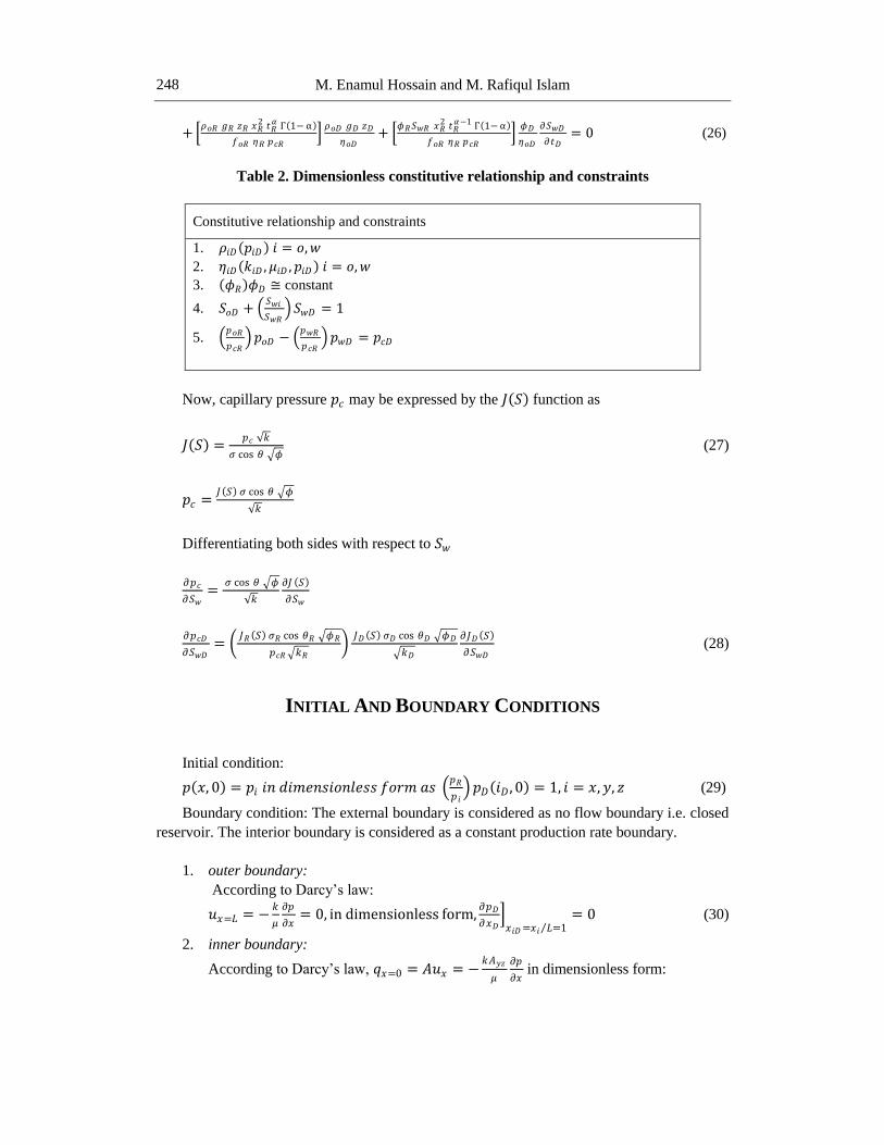
Now, capillary pressure 𝑝𝑐 may be expressed by the 𝐽 𝑆 function as
𝐽 𝑆 =𝑝𝑐 𝑘
𝜍 cos 𝜃 𝜙 (27)
𝑝𝑐 =𝐽 𝑆 𝜍 cos 𝜃 𝜙
𝑘
Differentiating both sides with respect to 𝑆𝑤
𝜕𝑝𝑐
𝜕𝑆𝑤=
𝜍 cos 𝜃 𝜙
𝑘
𝜕𝐽 𝑆
𝜕𝑆𝑤
𝜕𝑝𝑐𝐷
𝜕𝑆𝑤𝐷=
𝐽𝑅 𝑆 𝜍𝑅 cos 𝜃𝑅 𝜙𝑅
𝑝𝑐𝑅 𝑘𝑅
𝐽𝐷 𝑆 𝜍𝐷 cos 𝜃𝐷 𝜙𝐷
𝑘𝐷
𝜕𝐽𝐷 𝑆
𝜕𝑆𝑤𝐷 (28)
INITIAL AND BOUNDARY CONDITIONS
Initial condition:
𝑝 𝑥, 0 = 𝑝𝑖 𝑖𝑛 𝑑𝑖𝑚𝑒𝑛𝑠𝑖𝑜𝑛𝑙𝑒𝑠𝑠 𝑓𝑜𝑟𝑚 𝑎𝑠 𝑝𝑅
𝑝 𝑖 𝑝𝐷 𝑖𝐷 , 0 = 1, 𝑖 = 𝑥,𝑦, 𝑧 (29)
Boundary condition: The external boundary is considered as no flow boundary i.e. closed
reservoir. The interior boundary is considered as a constant production rate boundary.
1. outer boundary:
According to Darcy‟s law:
𝑢𝑥=𝐿 = −𝑘
𝜇
𝜕𝑝
𝜕𝑥= 0, in dimensionless form,
𝜕𝑝𝐷
𝜕𝑥𝐷 𝑥𝑖𝐷=𝑥𝑖 𝐿 =1
= 0 (30)
2. inner boundary:
According to Darcy‟s law, 𝑞𝑥=0 = 𝐴𝑢𝑥 = −𝑘𝐴𝑦𝑧
𝜇
𝜕𝑝
𝜕𝑥 in dimensionless form:
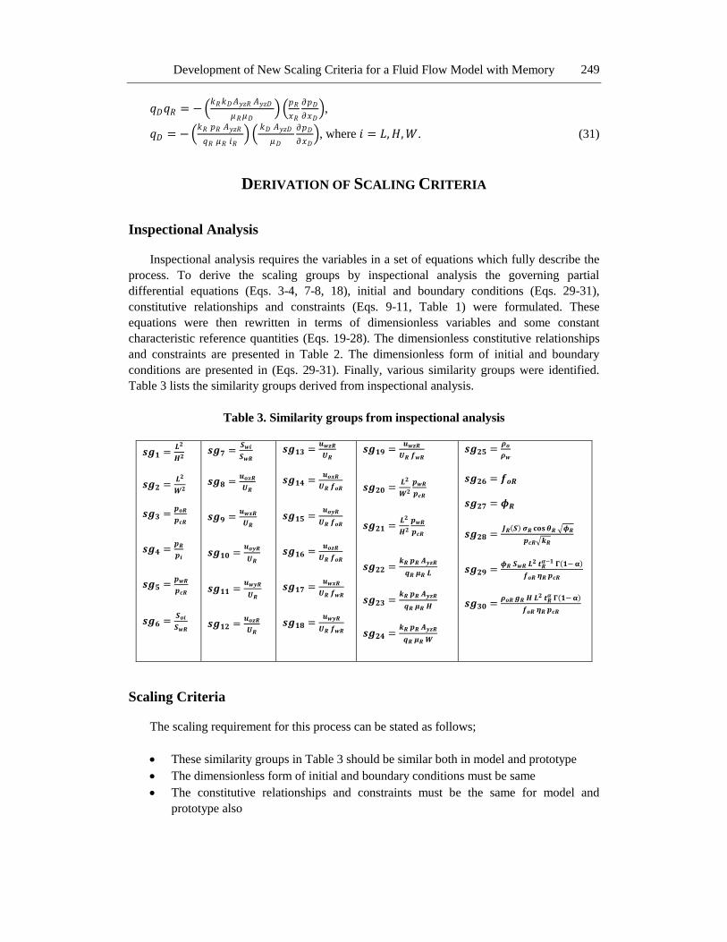
Development of New Scaling Criteria for a Fluid Flow Model with Memory 249
𝑞𝐷𝑞𝑅 = − 𝑘𝑅𝑘𝐷𝐴𝑦𝑧𝑅 𝐴𝑦𝑧𝐷
𝜇𝑅𝜇𝐷
𝑝𝑅
𝑥𝑅
𝜕𝑝𝐷
𝜕𝑥𝐷 ,
𝑞𝐷 = − 𝑘𝑅 𝑝𝑅 𝐴𝑦𝑧𝑅
𝑞𝑅 𝜇𝑅 𝑖𝑅
𝑘𝐷 𝐴𝑦𝑧𝐷
𝜇𝐷
𝜕𝑝𝐷
𝜕𝑥𝐷 , where 𝑖 = 𝐿,𝐻,𝑊. (31)
DERIVATION OF SCALING CRITERIA
Inspectional Analysis
Inspectional analysis requires the variables in a set of equations which fully describe the
process. To derive the scaling groups by inspectional analysis the governing partial
differential equations (Eqs. 3-4, 7-8, 18), initial and boundary conditions (Eqs. 29-31),
constitutive relationships and constraints (Eqs. 9-11, Table 1) were formulated. These
equations were then rewritten in terms of dimensionless variables and some constant
characteristic reference quantities (Eqs. 19-28). The dimensionless constitutive relationships
and constraints are presented in Table 2. The dimensionless form of initial and boundary
conditions are presented in (Eqs. 29-31). Finally, various similarity groups were identified.
Table 3 lists the similarity groups derived from inspectional analysis.
Table 3. Similarity groups from inspectional analysis
𝒔𝒈𝟏 =𝑳𝟐
𝑯𝟐
𝒔𝒈𝟐 =𝑳𝟐
𝑾𝟐
𝒔𝒈𝟑 =𝒑𝒐𝑹
𝒑𝒄𝑹
𝒔𝒈𝟒 =𝒑𝑹
𝒑𝒊
𝒔𝒈𝟓 =𝒑𝒘𝑹
𝒑𝒄𝑹
𝒔𝒈𝟔 =𝑺𝒐𝒊
𝑺𝒘𝑹
𝒔𝒈𝟕 =𝑺𝒘𝒊
𝑺𝒘𝑹
𝒔𝒈𝟖 =𝒖𝒐𝒙𝑹
𝑼𝑹
𝒔𝒈𝟗 =𝒖𝒘𝒙𝑹
𝑼𝑹
𝒔𝒈𝟏𝟎 =𝒖𝒐𝒚𝑹
𝑼𝑹
𝒔𝒈𝟏𝟏 =𝒖𝒘𝒚𝑹
𝑼𝑹
𝒔𝒈𝟏𝟐 =𝒖𝒐𝒛𝑹
𝑼𝑹
𝒔𝒈𝟏𝟑 =𝒖𝒘𝒛𝑹
𝑼𝑹
𝒔𝒈𝟏𝟒 =𝒖𝒐𝒙𝑹
𝑼𝑹 𝒇𝒐𝑹
𝒔𝒈𝟏𝟓 =𝒖𝒐𝒚𝑹
𝑼𝑹 𝒇𝒐𝑹
𝒔𝒈𝟏𝟔 =𝒖𝒐𝒛𝑹
𝑼𝑹 𝒇𝒐𝑹
𝒔𝒈𝟏𝟕 =𝒖𝒘𝒙𝑹
𝑼𝑹 𝒇𝒘𝑹
𝒔𝒈𝟏𝟖 =𝒖𝒘𝒚𝑹
𝑼𝑹 𝒇𝒘𝑹
𝒔𝒈𝟏𝟗 =𝒖𝒘𝒛𝑹
𝑼𝑹 𝒇𝒘𝑹
𝒔𝒈𝟐𝟎 =𝑳𝟐
𝑾𝟐
𝒑𝒘𝑹
𝒑𝒄𝑹
𝒔𝒈𝟐𝟏 =𝑳𝟐
𝑯𝟐
𝒑𝒘𝑹
𝒑𝒄𝑹
𝒔𝒈𝟐𝟐 =𝒌𝑹 𝒑𝑹 𝑨𝒚𝒛𝑹
𝒒𝑹 𝝁𝑹 𝑳
𝒔𝒈𝟐𝟑 =𝒌𝑹 𝒑𝑹 𝑨𝒚𝒛𝑹
𝒒𝑹 𝝁𝑹 𝑯
𝒔𝒈𝟐𝟒 =𝒌𝑹 𝒑𝑹 𝑨𝒚𝒛𝑹
𝒒𝑹 𝝁𝑹 𝑾
𝒔𝒈𝟐𝟓 =𝝆𝒐
𝝆𝒘
𝒔𝒈𝟐𝟔 = 𝒇𝒐𝑹
𝒔𝒈𝟐𝟕 = 𝝓𝑹
𝒔𝒈𝟐𝟖 = 𝑱𝑹 𝑺 𝝇𝑹 𝐜𝐨𝐬 𝜽𝑹 𝝓𝑹
𝒑𝒄𝑹 𝒌𝑹
𝒔𝒈𝟐𝟗 =𝝓𝑹 𝑺𝒘𝑹 𝑳𝟐 𝒕𝑹
𝜶−𝟏 𝚪 𝟏− 𝛂
𝒇𝒐𝑹 𝜼𝑹 𝒑𝒄𝑹
𝒔𝒈𝟑𝟎 =𝝆𝒐𝑹 𝒈𝑹 𝑯 𝑳𝟐 𝒕𝑹
𝜶 𝚪 𝟏− 𝛂
𝒇𝒐𝑹 𝜼𝑹 𝒑𝒄𝑹
Scaling Criteria
The scaling requirement for this process can be stated as follows;
These similarity groups in Table 3 should be similar both in model and prototype
The dimensionless form of initial and boundary conditions must be same
The constitutive relationships and constraints must be the same for model and
prototype also

M. Enamul Hossain and M. Rafiqul Islam 250
J(S) must be the same functions of the dimensionless saturation, 𝑆𝑤 .
Development of Relaxed Criteria
Based on the assumptions in the approach 1, the terms corresponding to these
assumptions (the terms that does not scale by the approach) are eliminated from the governing
equation shown in Eq. (25). Each term is then divided by one of the remaining coefficients to
yield the dimensionless form of equation. The coefficients represent the relaxed set of
similarity groups which can then be reduced to their simplest form. The constitutive
relationships, constraints, and initial and boundary conditions are treated in a similar manner.
For Approach 1, the effects of gravity are assumed negligible. For Approach 2, the effects the
vertical pressure gradient due to viscous and capillary forces is negligible. For Approach 3,
the effects of saturation, permeability, memory, the saturation pressure-saturation temperature
relationship and capillary forces are not scaled. For Approach 4, the effects capillary forces
are not scaled.
Approach 1. Same Porous Medium, Same Fluids, Same Pressure Drop, Same Temperature and Geometric Similarity
In this process, initial pressure and temperature as well as the maximum pressure and
temperature change must be same in the model and prototype. In addition, using the same
porous media (same porosity, same permeability, same grain size and same wettability) would
allow better scaling of the irreducible saturations and relative permeabilities. In our case, fluid
memory related to formation can be scaled properly and fluid memory related to formation
fluid can also be scaled properly due to same porous fluid. The main advantage of this
approach is to scale the properties such as viscosity, density, fluid memory and equilibrium
constants, which depend on pressure, temperature and composition of formation, are more
accurately scaled. Therefore, this approach would insure that viscous forces, capillary forces,
and diffusive forces are properly scaled while maintaining geometric similarity. However, it
does not allow the scaling of gravitational and dispersive effects. The relaxed sets of scaling
criteria for the approach are listed in Table 4. Here 𝑥𝑅 = 𝑦𝑅 = 𝑧𝑅 = 𝐿.
In addition of these scaling groups, all the dimensionless properties (Table 2) must be the
same function of their dimensionless variables for the prototype and model. For a model
reduced in length by a scaling factor “a” and employing the same fluids as the prototype:
Here, 𝑎 =𝐿𝑝𝑟𝑜𝑡𝑜 𝑡𝑦𝑝𝑒
𝐿𝑚𝑜𝑑𝑒𝑙 and
Δ𝑝𝑚𝑎𝑥 𝑝𝑚𝑎𝑥 − 𝑝𝑚𝑖𝑛 , 𝑝𝑜𝑖 , 𝑝𝑝𝑟𝑜𝑑𝑢𝑐𝑡𝑖𝑜𝑛 ,𝑇, 𝑘,𝑆𝑜𝑖 , 𝑆𝑤𝑖 , 𝜂𝑅 must be the same in model
and prototype
𝐻,𝑊, 𝑞 must be reduced by “a” from prototype to model
t will be reduced by 𝑎2 𝛼−1 from prototype to model
Approach 2. Same Porous Medium, Same Fluids, Same Pressure Drop, Same Temperature
and Relaxed Geometric Similarity
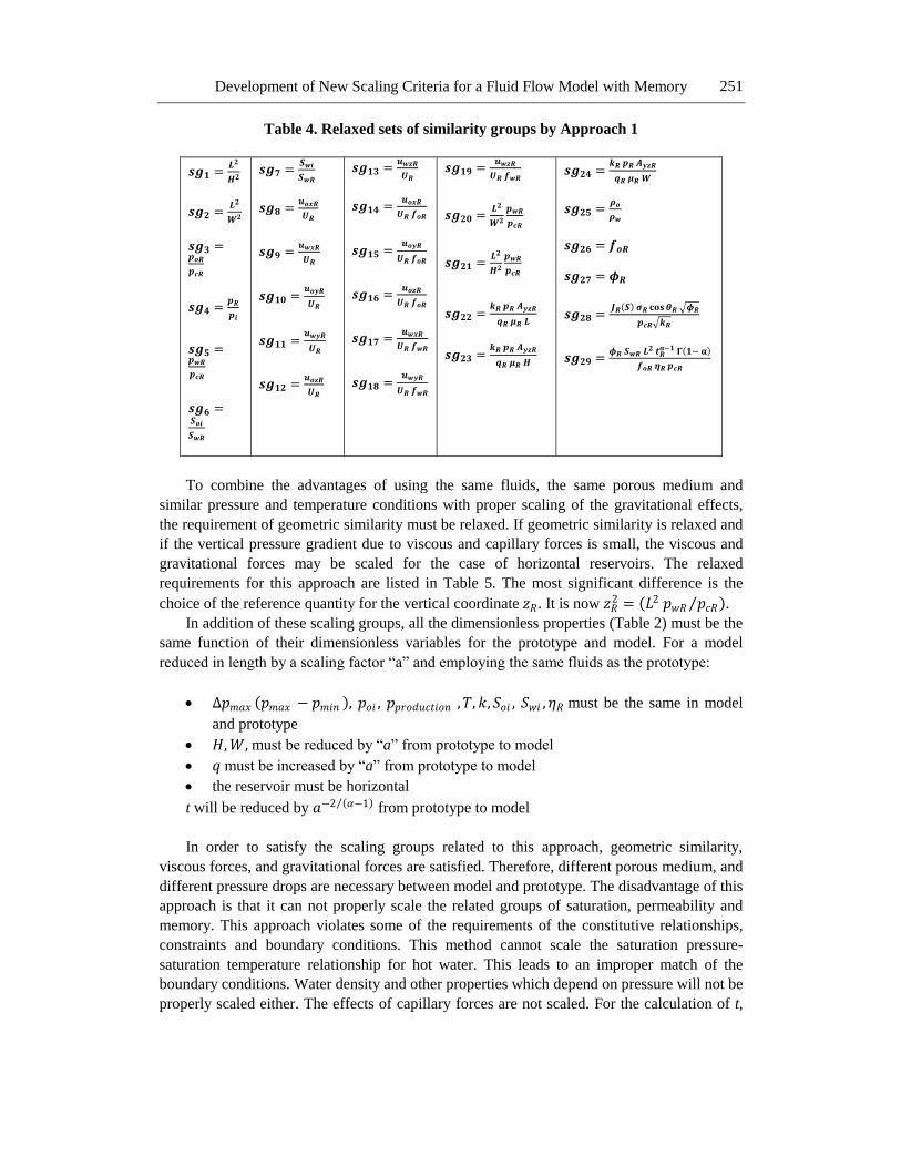
Development of New Scaling Criteria for a Fluid Flow Model with Memory 251
Table 4. Relaxed sets of similarity groups by Approach 1
𝒔𝒈𝟏 =𝑳𝟐
𝑯𝟐
𝒔𝒈𝟐 =𝑳𝟐
𝑾𝟐
𝒔𝒈𝟑 =𝒑𝒐𝑹
𝒑𝒄𝑹
𝒔𝒈𝟒 =𝒑𝑹
𝒑𝒊
𝒔𝒈𝟓 =𝒑𝒘𝑹
𝒑𝒄𝑹
𝒔𝒈𝟔 =𝑺𝒐𝒊
𝑺𝒘𝑹
𝒔𝒈𝟕 =𝑺𝒘𝒊
𝑺𝒘𝑹
𝒔𝒈𝟖 =𝒖𝒐𝒙𝑹
𝑼𝑹
𝒔𝒈𝟗 =𝒖𝒘𝒙𝑹
𝑼𝑹
𝒔𝒈𝟏𝟎 =𝒖𝒐𝒚𝑹
𝑼𝑹
𝒔𝒈𝟏𝟏 =𝒖𝒘𝒚𝑹
𝑼𝑹
𝒔𝒈𝟏𝟐 =𝒖𝒐𝒛𝑹
𝑼𝑹
𝒔𝒈𝟏𝟑 =𝒖𝒘𝒛𝑹
𝑼𝑹
𝒔𝒈𝟏𝟒 =𝒖𝒐𝒙𝑹
𝑼𝑹 𝒇𝒐𝑹
𝒔𝒈𝟏𝟓 =𝒖𝒐𝒚𝑹
𝑼𝑹 𝒇𝒐𝑹
𝒔𝒈𝟏𝟔 =𝒖𝒐𝒛𝑹
𝑼𝑹 𝒇𝒐𝑹
𝒔𝒈𝟏𝟕 =𝒖𝒘𝒙𝑹
𝑼𝑹 𝒇𝒘𝑹
𝒔𝒈𝟏𝟖 =𝒖𝒘𝒚𝑹
𝑼𝑹 𝒇𝒘𝑹
𝒔𝒈𝟏𝟗 =𝒖𝒘𝒛𝑹
𝑼𝑹 𝒇𝒘𝑹
𝒔𝒈𝟐𝟎 =𝑳𝟐
𝑾𝟐
𝒑𝒘𝑹
𝒑𝒄𝑹
𝒔𝒈𝟐𝟏 =𝑳𝟐
𝑯𝟐
𝒑𝒘𝑹
𝒑𝒄𝑹
𝒔𝒈𝟐𝟐 =𝒌𝑹 𝒑𝑹 𝑨𝒚𝒛𝑹
𝒒𝑹 𝝁𝑹 𝑳
𝒔𝒈𝟐𝟑 =𝒌𝑹 𝒑𝑹 𝑨𝒚𝒛𝑹
𝒒𝑹 𝝁𝑹 𝑯
𝒔𝒈𝟐𝟒 =𝒌𝑹 𝒑𝑹 𝑨𝒚𝒛𝑹
𝒒𝑹 𝝁𝑹 𝑾
𝒔𝒈𝟐𝟓 =𝝆𝒐
𝝆𝒘
𝒔𝒈𝟐𝟔 = 𝒇𝒐𝑹
𝒔𝒈𝟐𝟕 = 𝝓𝑹
𝒔𝒈𝟐𝟖 = 𝑱𝑹 𝑺 𝝇𝑹 𝐜𝐨𝐬𝜽𝑹 𝝓𝑹
𝒑𝒄𝑹 𝒌𝑹
𝒔𝒈𝟐𝟗 =𝝓𝑹 𝑺𝒘𝑹 𝑳𝟐 𝒕𝑹
𝜶−𝟏 𝚪 𝟏− 𝛂
𝒇𝒐𝑹 𝜼𝑹 𝒑𝒄𝑹
To combine the advantages of using the same fluids, the same porous medium and
similar pressure and temperature conditions with proper scaling of the gravitational effects,
the requirement of geometric similarity must be relaxed. If geometric similarity is relaxed and
if the vertical pressure gradient due to viscous and capillary forces is small, the viscous and
gravitational forces may be scaled for the case of horizontal reservoirs. The relaxed
requirements for this approach are listed in Table 5. The most significant difference is the
choice of the reference quantity for the vertical coordinate 𝑧𝑅. It is now 𝑧𝑅2 = 𝐿2 𝑝𝑤𝑅 𝑝𝑐𝑅 .
In addition of these scaling groups, all the dimensionless properties (Table 2) must be the
same function of their dimensionless variables for the prototype and model. For a model
reduced in length by a scaling factor “a” and employing the same fluids as the prototype:
Δ𝑝𝑚𝑎𝑥 𝑝𝑚𝑎𝑥 − 𝑝𝑚𝑖𝑛 , 𝑝𝑜𝑖 , 𝑝𝑝𝑟𝑜𝑑𝑢𝑐𝑡𝑖𝑜𝑛 ,𝑇, 𝑘,𝑆𝑜𝑖 , 𝑆𝑤𝑖 , 𝜂𝑅 must be the same in model
and prototype
𝐻,𝑊, must be reduced by “a” from prototype to model
𝑞 must be increased by “a” from prototype to model
the reservoir must be horizontal
t will be reduced by 𝑎−2 𝛼−1 from prototype to model
In order to satisfy the scaling groups related to this approach, geometric similarity,
viscous forces, and gravitational forces are satisfied. Therefore, different porous medium, and
different pressure drops are necessary between model and prototype. The disadvantage of this
approach is that it can not properly scale the related groups of saturation, permeability and
memory. This approach violates some of the requirements of the constitutive relationships,
constraints and boundary conditions. This method cannot scale the saturation pressure-
saturation temperature relationship for hot water. This leads to an improper match of the
boundary conditions. Water density and other properties which depend on pressure will not be
properly scaled either. The effects of capillary forces are not scaled. For the calculation of t,
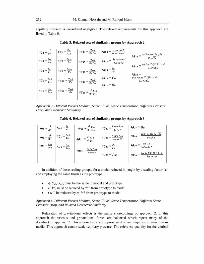
M. Enamul Hossain and M. Rafiqul Islam 252
capillary pressure is considered negligible. The relaxed requirements for this approach are
listed in Table 6.
Table 5. Relaxed sets of similarity groups by Approach 2
𝒔𝒈𝟐 =𝑳𝟐
𝑾𝟐
𝒔𝒈𝟑 =𝒑𝒐𝑹
𝒑𝒄𝑹
𝒔𝒈𝟒 =𝒑𝑹
𝒑𝒊
𝒔𝒈𝟓 =𝒑𝒘𝑹
𝒑𝒄𝑹
𝒔𝒈𝟔 =𝑺𝒐𝒊
𝑺𝒘𝑹
𝒔𝒈𝟕 =𝑺𝒘𝒊
𝑺𝒘𝑹
𝒔𝒈𝟖 =𝒖𝒐𝒙𝑹
𝑼𝑹
𝒔𝒈𝟗 =𝒖𝒘𝒙𝑹
𝑼𝑹
𝒔𝒈𝟏𝟎 =𝒖𝒐𝒚𝑹
𝑼𝑹
𝒔𝒈𝟏𝟏 =𝒖𝒘𝒚𝑹
𝑼𝑹
𝒔𝒈𝟏𝟒 =𝒖𝒐𝒙𝑹
𝑼𝑹 𝒇𝒐𝑹
𝒔𝒈𝟏𝟓 =𝒖𝒐𝒚𝑹
𝑼𝑹 𝒇𝒐𝑹
𝒔𝒈𝟏𝟕 =𝒖𝒘𝒙𝑹
𝑼𝑹 𝒇𝒘𝑹
𝒔𝒈𝟏𝟖 =𝒖𝒘𝒚𝑹
𝑼𝑹 𝒇𝒘𝑹
𝒔𝒈𝟐𝟎 =𝑳𝟐
𝑾𝟐
𝒑𝒘𝑹
𝒑𝒄𝑹
𝒔𝒈𝟐𝟐 = 𝒌𝑹 𝒑𝑹 𝒑𝒘𝑹 𝑾
𝒒𝑹 𝝁𝑹 𝒑𝒄𝑹 𝑳𝟐
𝒔𝒈𝟐𝟒 = 𝒌𝑹 𝒑𝑹 𝒑𝒘𝑹 𝑳𝟐
𝒑𝒄𝑹 𝒒𝑹 𝝁𝑹
𝒔𝒈𝟐𝟓 =𝝆𝒐
𝝆𝒘
𝒔𝒈𝟐𝟔 = 𝒇𝒐𝑹
𝒔𝒈𝟐𝟕 = 𝝓𝑹
𝒔𝒈𝟐𝟖 = 𝑱𝑹 𝑺 𝝇𝑹 𝐜𝐨𝐬 𝜽𝑹 𝝓𝑹
𝒑𝒄𝑹 𝒌𝑹
𝒔𝒈𝟐𝟗 =𝝓𝑹 𝑺𝒘𝑹 𝑳𝟐 𝒕𝑹
𝜶−𝟏 𝚪 𝟏− 𝛂
𝒇𝒐𝑹 𝜼𝑹 𝒑𝒄𝑹
𝒔𝒈𝟑𝟎 = 𝒑𝒘𝑹 𝝆𝒐𝑹 𝒈𝑹 𝑳𝟒 𝒕𝑹
𝜶 𝚪 𝟏− 𝛂
𝒇𝒐𝑹 𝜼𝑹 𝒑𝒄𝑹𝟐
Approach 3. Different Porous Medium, Same Fluids, Same Temperature, Different Pressure Drop, and Geometric Similarity
Table 6. Relaxed sets of similarity groups by Approach 3
𝒔𝒈𝟏 =𝑳𝟐
𝑯𝟐
𝒔𝒈𝟐 =𝑳𝟐
𝑾𝟐
𝒔𝒈𝟑 =𝒑𝒐𝑹
𝒑𝒄𝑹
𝐬𝒈𝟒 =𝒑𝑹
𝒑𝒊
𝒔𝒈𝟓 =𝒑𝒘𝑹
𝒑𝒄𝑹
𝒔𝒈𝟔 =𝑺𝒐𝒊
𝑺𝒘𝑹
𝒔𝒈𝟐𝟎 =𝑳𝟐
𝑾𝟐
𝒑𝒘𝑹
𝒑𝒄𝑹
𝒔𝒈𝟐𝟏 =𝑳𝟐
𝑯𝟐
𝒑𝒘𝑹
𝒑𝒄𝑹
𝒔𝒈𝟐𝟐 =𝒌𝑹 𝒑𝑹 𝑨𝒚𝒛𝑹
𝒒𝑹 𝝁𝑹 𝑳
𝒔𝒈𝟐𝟑 =𝒌𝑹 𝒑𝑹 𝑨𝒚𝒛𝑹
𝒒𝑹 𝝁𝑹 𝑯
𝒔𝒈𝟐𝟒 =𝒌𝑹 𝒑𝑹 𝑨𝒚𝒛𝑹
𝒒𝑹 𝝁𝑹 𝑾
𝒔𝒈𝟐𝟓 =𝝆𝒐
𝝆𝒘
𝒔𝒈𝟐𝟔 = 𝒇𝒐𝑹
𝒔𝒈𝟐𝟕 = 𝝓𝑹
𝒔𝒈𝟐𝟖 = 𝑱𝑹 𝑺 𝝇𝑹 𝐜𝐨𝐬 𝜽𝑹 𝝓𝑹
𝒑𝒄𝐑 𝒌𝑹
𝒔𝒈𝟐𝟗 =𝝓𝑹 𝑺𝒘𝑹
𝒕𝑹 𝝆𝒐𝑹 𝒈𝑹 𝑾
𝒔𝒈𝟑𝟎 =𝝆𝒐𝑹 𝒈𝑹 𝑯 𝑳𝟐 𝒕𝑹
𝜶 𝚪 𝟏− 𝛂
𝒇𝒐𝑹 𝜼𝑹 𝒑𝒄𝑹
In addition of these scaling groups, for a model reduced in length by a scaling factor “a”
and employing the same fluids as the prototype:
ϕ,𝑆𝑜𝑖 , 𝑆𝑤𝑖 , must be the same in model and prototype
𝐻,𝑊, must be reduced by “a” from prototype to model
t will be reduced by 𝑎−3 𝛼 from prototype to model
Approach 4. Different Porous Medium, Same Fluids, Same Temperature, Different Same
Pressure Drop, and Relaxed Geometric Similarity
Relaxation of gravitational effects is the major shortcomings of approach 2. In this
approach the viscous and gravitational forces are balanced which repeat many of the
drawback of approach 3. This is done by relaxing pressure drop and requires different porous
media. This approach cannot scale capillary pressure. The reference quantity for the vertical
Development of New Scaling Criteria for a Fluid Flow Model with Memory 253
coordinate 𝑧𝑅 is calculated by setting the ratio of vertical and length distance ratio equals one.
It is now 𝑧𝑅2 = 𝐿2. The main disadvantage of this approach is that time is scaled up by the
factor “a”. This indicates that experimental time is more than that of field. The relaxed
requirements for this approach are listed in Table 7.
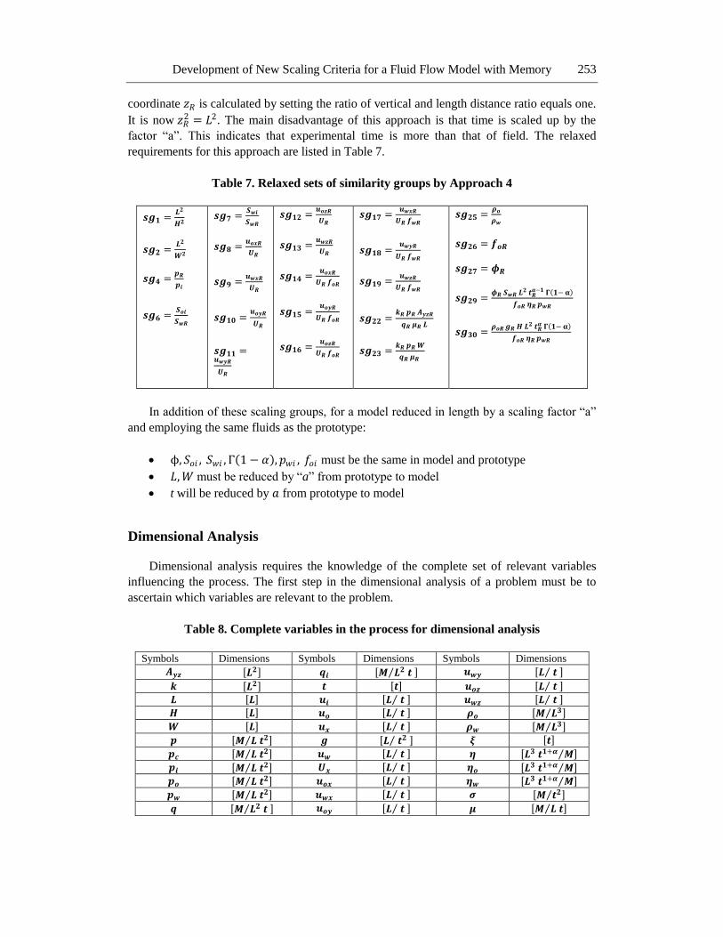
Table 7. Relaxed sets of similarity groups by Approach 4
𝒔𝒈𝟏 =𝑳𝟐
𝑯𝟐
𝒔𝒈𝟐 =𝑳𝟐
𝑾𝟐
𝒔𝒈𝟒 =𝒑𝑹
𝒑𝒊
𝒔𝒈𝟔 =𝑺𝒐𝒊
𝑺𝒘𝑹
𝒔𝒈𝟕 =𝑺𝒘𝒊
𝑺𝒘𝑹
𝒔𝒈𝟖 =𝒖𝒐𝒙𝑹
𝑼𝑹
𝒔𝒈𝟗 =𝒖𝒘𝒙𝑹
𝑼𝑹
𝒔𝒈𝟏𝟎 =𝒖𝒐𝒚𝑹
𝑼𝑹
𝒔𝒈𝟏𝟏 =𝒖𝒘𝒚𝑹
𝑼𝑹
𝒔𝒈𝟏𝟐 =𝒖𝒐𝒛𝑹
𝑼𝑹
𝒔𝒈𝟏𝟑 =𝒖𝒘𝒛𝑹
𝑼𝑹
𝒔𝒈𝟏𝟒 =𝒖𝒐𝒙𝑹
𝑼𝑹 𝒇𝒐𝑹
𝒔𝒈𝟏𝟓 =𝒖𝒐𝒚𝑹
𝑼𝑹 𝒇𝒐𝑹
𝒔𝒈𝟏𝟔 =𝒖𝒐𝒛𝑹
𝑼𝑹 𝒇𝒐𝑹
𝒔𝒈𝟏𝟕 =𝒖𝒘𝒙𝑹
𝑼𝑹 𝒇𝒘𝑹
𝒔𝒈𝟏𝟖 =𝒖𝒘𝒚𝑹
𝑼𝑹 𝒇𝒘𝑹
𝒔𝒈𝟏𝟗 =𝒖𝒘𝒛𝑹
𝑼𝑹 𝒇𝒘𝑹
𝒔𝒈𝟐𝟐 =𝒌𝑹 𝒑𝑹 𝑨𝒚𝒛𝑹
𝒒𝑹 𝝁𝑹 𝑳
𝒔𝒈𝟐𝟑 =𝒌𝑹 𝒑𝑹 𝑾
𝒒𝑹 𝝁𝑹
𝒔𝒈𝟐𝟓 =𝝆𝒐
𝝆𝒘
𝒔𝒈𝟐𝟔 = 𝒇𝒐𝑹
𝒔𝒈𝟐𝟕 = 𝝓𝑹
𝒔𝒈𝟐𝟗 =𝝓𝑹 𝑺𝒘𝑹 𝑳𝟐 𝒕𝑹
𝜶−𝟏 𝚪 𝟏− 𝛂
𝒇𝒐𝑹 𝜼𝑹 𝒑𝒘𝑹
𝒔𝒈𝟑𝟎 =𝝆𝒐𝑹 𝒈𝑹 𝑯 𝑳𝟐 𝒕𝑹
𝜶 𝚪 𝟏− 𝛂
𝒇𝒐𝑹 𝜼𝑹 𝒑𝒘𝑹
In addition of these scaling groups, for a model reduced in length by a scaling factor “a”
and employing the same fluids as the prototype:
ϕ,𝑆𝑜𝑖 , 𝑆𝑤𝑖 ,Γ 1 − 𝛼 ,𝑝𝑤𝑖 , 𝑓𝑜𝑖 must be the same in model and prototype
𝐿,𝑊 must be reduced by “a” from prototype to model
t will be reduced by 𝑎 from prototype to model
Dimensional Analysis
Dimensional analysis requires the knowledge of the complete set of relevant variables
influencing the process. The first step in the dimensional analysis of a problem must be to
ascertain which variables are relevant to the problem.
Table 8. Complete variables in the process for dimensional analysis
Symbols Dimensions Symbols Dimensions Symbols Dimensions
𝑨𝒚𝒛 𝑳𝟐 𝒒𝒊 𝑴 𝑳𝟐 𝒕 𝒖𝒘𝒚 𝑳 𝒕
𝒌 𝑳𝟐 𝒕 𝒕 𝒖𝒐𝒛 𝑳 𝒕
𝑳 𝑳 𝒖𝒊 𝑳 𝒕 𝒖𝒘𝒛 𝑳 𝒕
𝑯 𝑳 𝒖𝒐 𝑳 𝒕 𝝆𝒐 𝑴 𝑳𝟑
𝑾 𝑳 𝒖𝒙 𝑳 𝒕 𝝆𝒘 𝑴 𝑳𝟑
𝒑 𝑴 𝑳 𝒕𝟐 𝒈 𝑳 𝒕𝟐 𝝃 𝒕
𝒑𝒄 𝑴 𝑳 𝒕𝟐 𝒖𝒘 𝑳 𝒕 𝜼 𝑳𝟑 𝒕𝟏+𝜶 𝑴 𝒑𝒊 𝑴 𝑳 𝒕𝟐 𝑼𝒙 𝑳 𝒕 𝜼𝒐 𝑳𝟑 𝒕𝟏+𝜶 𝑴 𝒑𝒐 𝑴 𝑳 𝒕𝟐 𝒖𝒐𝒙 𝑳 𝒕 𝜼𝒘 𝑳𝟑 𝒕𝟏+𝜶 𝑴
𝒑𝒘 𝑴 𝑳 𝒕𝟐 𝒖𝒘𝒙 𝑳 𝒕 𝝇 𝑴 𝒕𝟐
𝒒 𝑴 𝑳𝟐 𝒕 𝒖𝒐𝒚 𝑳 𝒕 𝝁 𝑴 𝑳 𝒕

M. Enamul Hossain and M. Rafiqul Islam 254
Special care should be exercised at this stage that all the relevant variables are included.
This analysis often yields a more complete set of similarity groups but the physical meaning
of the similarity groups themselves is generally more apparent from inspectional analysis.
Dimensional analysis is usually used in conjunction with inspectional analysis to ensure
important groups are not omitted. The similarity groups may also be derived using
dimensional analysis. After the relevant variables for the process are selected, the similarity
groups can be determined using the Buckingham π-theorem. Table 8 lists the symbols,
dimensions of the variables selected. Table 9 shows the similarity groups derived by this
method. There are some more scaling groups identified by dimensional analysis. These are
𝜋1, 𝜋10, 𝜋11, 𝜋23, 𝜋26, 𝜋27, 𝜋28, 𝜋30.
RESULTS AND DISCUSSION
To find out the displacement efficiency of the application of different Approaches,
pressure drop and time are considered as the principle criteria in the selection of scaling laws.
When fluid memory is being encountered, it is necessary to select an appropriate Approach to
scale the different parameters from lab to field or vice versa. In solving different similarity
groups, 𝛼 = 0.1 𝑎𝑛𝑑 0.2,𝜙 = 0.3, 𝑆𝑤 = 0.24,𝜂 = 0.343249,𝜌0 = 50.0 𝑙𝑏𝑚 𝑓𝑡3 , L =
1000.0 ft, 𝑊 = 400.0 𝑓𝑡,𝐻 = 50.0 𝑓𝑡, 𝑝𝑐 = 30.0 𝑝𝑠𝑖,𝑔 = 32.2 𝑓𝑡 𝑠2 ,𝑓0 = 0.2,𝑝𝑖 =
3000.0 𝑝𝑠𝑖, and a pressure drop of 0 ~ 320 𝑝𝑠𝑖 have been regarded.
Approach 1
Equating the similarity groups Group 3 and Group 29 becomes;
𝑠𝑔3 = 𝑠𝑔29 ⇒ 𝑝𝑜𝑅
𝑝𝑐𝑅=
𝜙𝑅 𝑆𝑤𝑅 𝐿2 𝑡𝑅𝛼−1 Γ 1− α
𝑓𝑜𝑅 𝜂𝑅 𝑝𝑐𝑅
𝑝𝑜𝑅 =𝜙𝑅 𝑆𝑤𝑅 𝐿2 𝑡𝑅
𝛼−1 Γ 1− α
𝑓𝑜𝑅 𝜂𝑅
𝑡𝑅𝛼−1 =
𝑓𝑜𝑅 𝜂𝑅 𝑝𝑜𝑅
𝜙𝑅 𝑆𝑤𝑅 𝐿2 Γ 1− α
𝑡𝑅 = 𝑓𝑜𝑅 𝜂𝑅 𝑝𝑜𝑅
𝜙𝑅 𝑆𝑤𝑅 𝐿2 Γ 1− α
1 𝛼−1
(32)
Figure 1 shows the variation of pressure drop with time for different fraction
derivative, 𝛼, values when Approach 1 is considered. Equation (32) is used in developing this
plotting. The graph shows that pressure drop decreases with time from a reference point
which has a non-linear trend. There is a huge pressure drop at the beginning of oil-water
displacement process.
This gap gradually decreases with time. Moreover, α has a great role in displacement
process. When α increases pressure drop delays during the process. This simply means that
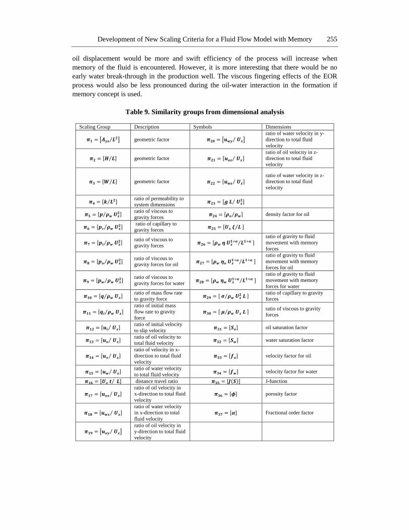
Development of New Scaling Criteria for a Fluid Flow Model with Memory 255
oil displacement would be more and swift efficiency of the process will increase when
memory of the fluid is encountered. However, it is more interesting that there would be no
early water break-through in the production well. The viscous fingering effects of the EOR
process would also be less pronounced during the oil-water interaction in the formation if
memory concept is used.
Table 9. Similarity groups from dimensional analysis
Scaling Group Description Symbols Dimensions
𝝅𝟏 = 𝑨𝒚𝒛 𝑳𝟐 geometric factor 𝝅𝟐𝟎 = 𝒖𝒘𝒚 𝑼𝒙 ratio of water velocity in y-
direction to total fluid
velocity
𝝅𝟐 = 𝑯 𝑳 geometric factor 𝝅𝟐𝟏 = 𝒖𝒐𝒛 𝑼𝒙 ratio of oil velocity in z-direction to total fluid
velocity
𝝅𝟑 = 𝑾 𝑳 geometric factor 𝝅𝟐𝟐 = 𝒖𝒘𝒛 𝑼𝒙 ratio of water velocity in z-direction to total fluid
velocity
𝝅𝟒 = 𝒌 𝑳𝟐 ratio of permeability to system dimensions
𝝅𝟐𝟑 = 𝒈 𝑳 𝑼𝒙𝟐
𝝅𝟓 = 𝒑 𝝆𝒘 𝑼𝒙𝟐
ratio of viscous to
gravity forces 𝝅𝟐𝟒 = 𝝆𝒐 𝝆𝒘 density factor for oil
𝝅𝟔 = 𝒑𝒄 𝝆𝒘 𝑼𝒙𝟐
ratio of capillary to gravity forces
𝝅𝟐𝟓 = 𝑼𝒙 𝝃 𝑳
𝝅𝟕 = 𝒑𝒊 𝝆𝒘 𝑼𝒙𝟐
ratio of viscous to gravity forces
𝝅𝟐𝟔 = 𝝆𝒘 𝜼 𝑼𝒙𝟏+𝜶 𝑳𝟏+𝜶
ratio of gravity to fluid
movement with memory
forces
𝝅𝟖 = 𝒑𝒐 𝝆𝒘 𝑼𝒙𝟐
ratio of viscous to gravity forces for oil
𝝅𝟐𝟕 = 𝝆𝒘 𝜼𝒐 𝑼𝒙𝟏+𝜶 𝑳𝟏+𝜶
ratio of gravity to fluid
movement with memory
forces for oil
𝝅𝟗 = 𝒑𝒘 𝝆𝒘 𝑼𝒙𝟐
ratio of viscous to
gravity forces for water 𝝅𝟐𝟖 = 𝝆𝒘 𝜼𝒘 𝑼𝒙
𝟏+𝜶 𝑳𝟏+𝜶 ratio of gravity to fluid movement with memory
forces for water
𝝅𝟏𝟎 = 𝒒 𝝆𝒘 𝑼𝒙 ratio of mass flow rate to gravity force
𝝅𝟐𝟗 = 𝝇 𝝆𝒘 𝑼𝒙𝟐 𝑳
ratio of capillary to gravity forces
𝝅𝟏𝟏 = 𝒒𝒊 𝝆𝒘 𝑼𝒙 ratio of initial mass
flow rate to gravity
force 𝝅𝟑𝟎 = 𝝁 𝝆𝒘 𝑼𝒙 𝑳
ratio of viscous to gravity forces
𝝅𝟏𝟐 = 𝒖𝒊 𝑼𝒙 ratio of initial velocity
to slip velocity 𝝅𝟑𝟏 = 𝑺𝒐 oil saturation factor
𝝅𝟏𝟑 = 𝒖𝒐 𝑼𝒙 ratio of oil velocity to total fluid velocity
𝝅𝟑𝟐 = 𝑺𝒘 water saturation factor
𝝅𝟏𝟒 = 𝒖𝒙 𝑼𝒙 ratio of velocity in x-
direction to total fluid
velocity 𝝅𝟑𝟑 = 𝒇𝒐 velocity factor for oil
𝝅𝟏𝟓 = 𝒖𝒘 𝑼𝒙 ratio of water velocity
to total fluid velocity 𝝅𝟑𝟒 = 𝒇𝒘 velocity factor for water
𝝅𝟏𝟔 = 𝑼𝒙 𝒕 𝑳 distance travel ratio 𝝅𝟑𝟓 = 𝑱 𝑺 J-function
𝝅𝟏𝟕 = 𝒖𝒐𝒙 𝑼𝒙 ratio of oil velocity in
x-direction to total fluid
velocity 𝝅𝟑𝟔 = 𝝓 porosity factor
𝝅𝟏𝟖 = 𝒖𝒘𝒙 𝑼𝒙 ratio of water velocity
in x-direction to total
fluid velocity 𝝅𝟑𝟕 = 𝜶 Fractional order factor
𝝅𝟏𝟗 = 𝒖𝒐𝒚 𝑼𝒙 ratio of oil velocity in y-direction to total fluid
velocity

M. Enamul Hossain and M. Rafiqul Islam 256
Figure 1. Variation of pressure drop with time for Approach 1.
Approach 2
Equating the similarity groups Group 20 and Group 29 becomes;
𝑠𝑔21 = 𝑠𝑔29 ⇒ 𝐿2
𝑊2
𝑝𝑤𝑅
𝑝𝑐𝑅=
𝜙𝑅 𝑆𝑤𝑅 𝐿2 𝑡𝑅𝛼−1 Γ 1− α
𝑓𝑜𝑅 𝜂𝑅 𝑝𝑐𝑅
𝑡𝑅𝛼−1 =
𝑝𝑤𝑅 𝑓𝑜𝑅 𝜂𝑅
𝑊2𝜙𝑅 𝑆𝑤𝑅 Γ 1 − α
𝑡𝑅 = 𝑝𝑤𝑅 𝑓𝑜𝑅 𝜂𝑅
𝑊2𝜙𝑅 𝑆𝑤𝑅 Γ 1− α
1 𝛼−1
(33)
Figure 2 shows the variation of pressure drop vs. time for different α values when
Approach 2 is considered. Equation (33) is used in developing this plotting. The trend and
nature of the graph is same as explained for Approach 1 except the time duration of the
process. When Approach 2 is used, it takes less time to complete the displacement process
comparing with Approach 1.
0 2000 4000 6000 8000 10000 12000 14000 16000 180000
50
100
150
200
250
300
350
Time (t), days
Pre
ssu
re d
rop
(
p),
psi
= 0.1
= 0.2

Development of New Scaling Criteria for a Fluid Flow Model with Memory 257
Figure 2. Variation of pressure drop with time for Approach 2.
Approach 3
Equating the similarity groups Group 21 and Group 29 becomes;
𝑠𝑔21 = 𝑠𝑔29 ⇒𝐿2
𝐻2
𝑝𝑤𝑅
𝑝𝑐𝑅=
𝜙𝑅 𝑆𝑤𝑅
𝑡𝑅 𝜌𝑜𝑅 𝑔𝑅 𝑊
𝑡𝑅 =𝜙𝑅 𝑆𝑤𝑅 𝐻2 𝑝𝑐𝑅
𝜌𝑜𝑅 𝑔𝑅 𝑊 𝐿2 𝑝𝑤𝑅 (34)
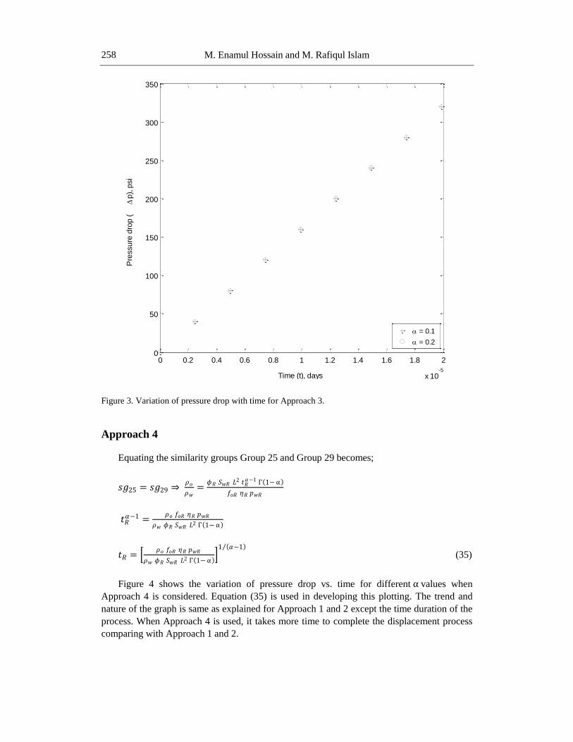
Figure 3 shows the variation of pressure drop with time for different α values when
Approach 3 is considered. Equation (34) is used in developing this plotting. The graph shows
that pressure drop increases with time from a reference point. It should be noted that there is
no memory effects in this Approach. Here, the time domain is very short during the
displacement process and pressure drop varies linearly with time.
This Approach indicates that, if memory effect is ignored, oil displacement would not be
more and swift efficiency of the process will be lesser than that of Approaches based on
memory. Moreover, early water break-through in the production well will be traced and
viscous fingering effects of the EOR process will be stronger than that of memory based
Approaches.
0 200 400 600 800 1000 1200 1400 1600 18000
50
100
150
200
250
300
350
Time (t), days
Pre
ssu
re d
rop
(
p),
psi
= 0.1
= 0.2
M. Enamul Hossain and M. Rafiqul Islam 258
Figure 3. Variation of pressure drop with time for Approach 3.
Approach 4
Equating the similarity groups Group 25 and Group 29 becomes;
𝑠𝑔25 = 𝑠𝑔29 ⇒ 𝜌𝑜
𝜌𝑤=
𝜙𝑅 𝑆𝑤𝑅 𝐿2 𝑡𝑅𝛼−1 Γ 1− α
𝑓𝑜𝑅 𝜂𝑅 𝑝𝑤𝑅
𝑡𝑅𝛼−1 =
𝜌𝑜 𝑓𝑜𝑅 𝜂𝑅 𝑝𝑤𝑅
𝜌𝑤 𝜙𝑅 𝑆𝑤𝑅 𝐿2 Γ 1− α
𝑡𝑅 = 𝜌𝑜 𝑓𝑜𝑅 𝜂𝑅 𝑝𝑤𝑅
𝜌𝑤 𝜙𝑅 𝑆𝑤𝑅 𝐿2 Γ 1− α
1 𝛼−1
(35)
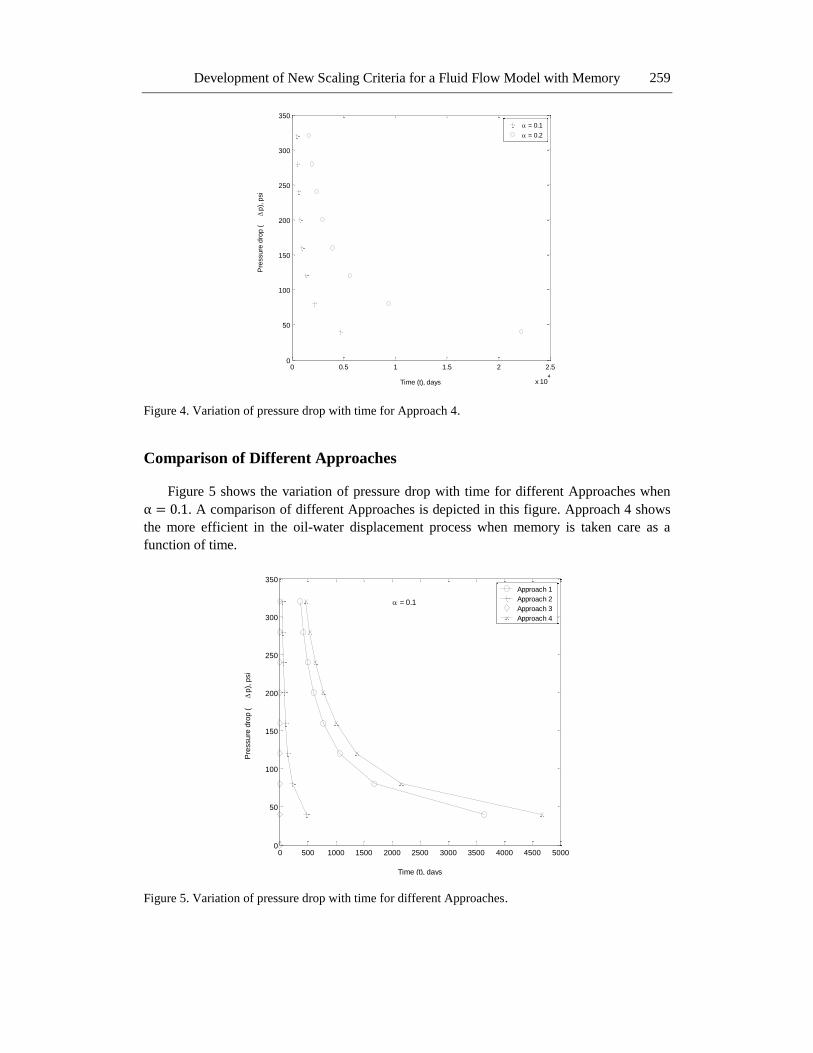
Figure 4 shows the variation of pressure drop vs. time for different α values when
Approach 4 is considered. Equation (35) is used in developing this plotting. The trend and
nature of the graph is same as explained for Approach 1 and 2 except the time duration of the
process. When Approach 4 is used, it takes more time to complete the displacement process
comparing with Approach 1 and 2.
0 0.2 0.4 0.6 0.8 1 1.2 1.4 1.6 1.8 2
x 10-5
0
50
100
150
200
250
300
350
Time (t), days
Pre
ssu
re d
rop
(
p),
psi
= 0.1
= 0.2
Development of New Scaling Criteria for a Fluid Flow Model with Memory 259
Figure 4. Variation of pressure drop with time for Approach 4.
Comparison of Different Approaches
Figure 5 shows the variation of pressure drop with time for different Approaches when
α = 0.1. A comparison of different Approaches is depicted in this figure. Approach 4 shows
the more efficient in the oil-water displacement process when memory is taken care as a
function of time.
Figure 5. Variation of pressure drop with time for different Approaches.
0 0.5 1 1.5 2 2.5
x 104
0
50
100
150
200
250
300
350
Time (t), days
Pre
ssu
re d
rop
(
p),
psi
= 0.1
= 0.2
0 500 1000 1500 2000 2500 3000 3500 4000 4500 50000
50
100
150
200
250
300
350
Time (t), days
Pre
ssu
re d
rop
(
p),
psi
Approach 1
Approach 2
Approach 3
Approach 4
= 0.1

M. Enamul Hossain and M. Rafiqul Islam 260
Approach 1 is also efficient comparing with Approaches 2 and 3. The use of Approach 3
does not give any significant information during the process when memory of the fluid is
disregarded. It is better to use Approach 4 or Approach 1 in the case of memory reflection.
CONCLUSIONS
This paper introduces new scaling criteria for oil-water displacement based on the
implementation of memory concept. Relaxed sets of similarity groups and a complete set of
similarity groups have also been identified. An efficient Approach is outlined for oil-water
displacement process with memory. The choice of a subset is considered based on uniform
porosities, pressure drop and geometrical similarities. The subset of the dimensionless groups
neglected the effect of dispersive forces. However, future scaled up experimental studies will
provide a deeper insight into the fluid-fluid interactions at a scaled up level and this paper
may be a guidance to reduce considerable expenditures associated with oil-water
displacement process in an EOR scheme. In future, the lab experimental results based on
memory concept can be used to predict field performance in petroleum industry.
ACKNOWLEDGMENTS
The authors would like to thank the Atlantic Canada Opportunities Agency (ACOA) for
funding this project under the Atlantic Innovation Fund (AIF). The first author would also
like to thank Natural Sciences and Engineering Research Council of Canada (NSERC) for
funding.
REFERENCES
Bansal, A. and Islam, M.R. 1994. Scaled Model Studies of Heavy Oil Recovery from an
Alaskan Reservoir Using Gravity-assisted Gas Injection. J of Canadian Petroleum
Technology. 33 (6): 52 – 61, June.
Basu, A. and Islam, M.R. 2007. Scaling up of Chemical Injection Experiments. Petroleum
Science and Technology, in press.
Coskuner, G. and Bentsen, R.G. 1988. Hele Shaw Cell Study of a new approach to instability
theory in porous media. J. of Canadian Petroleum Technology. 27(1): 87 – 95.
Farouq Ali, S.M. and Redford, D.A. 1977. Physical Modeling of In Situ Recovery Methods
for Oil Sands. Oil Sands. 319 – 325.
Farouq Ali, S.M., Redford, D.A. and Islam, M.R. 1987. Scaling Laws for Enhanced Oil
Recovery Experiments. China-Canada Joint Technical Conference on Heavy Oil
Recovery. Zhou Zhou City, China.
Geertsma, J., Croes, G.A., and Schwarz. 1956. Theory of Dimensionally Scaled Models of
Petroleum Reservoirs. Petroleum Trans., AIME, 207: 118 – 127.
Hossain, M. E., Ketata, C., and Islam, M. R. 2009a. A Scaled Model Study of Waterjet
Drilling. Petroleum Science and Technology, 27, pp. 1261 – 1273.
Development of New Scaling Criteria for a Fluid Flow Model with Memory 261
Hossain, M. E., Mousavizadegan, S. H. and Islam, M. R. 2009b. Effects of Memory on the
Complex Rock-Fluid Properties of a Reservoir Stress-Strain Model. Petroleum Science
and Technology, 27 (10), pp. 1109 – 1123.
Hossain, M E., Mousavizadegan, S. H. and Islam, M. R. 2008. A Novel Fluid Flow Model
with Memory for Porous Media Applications. MTDM Conference 2008, Mechanics of
Time Dependent Materials Conference, March 30 - April 4, 2008, Monterey, California.
Hossain, M. E., Mousavizadegan, S. H. and Islam, M. R. 2007. A Novel Memory Based
Stress-Strain Model for Reservoir Characterization. Journal Nature Science and
Sustainable Technology, Volume 1(4), pp. 653 – 678.
Islam, M.R. 1987. Mobility Control in Waterflooding Oil Reservoirs with a Bottom- Water
Zone. PhD dissertation, Department of Mining, Metallurgical and Petroleum
Engineering, U of Alberta, Edmonton, Alberta, Canada.
Islam, M.R. and Farouq Ali, S.M. 1990. New Scaling Criteria for Chemical Flooding
Experiments. J. of Canadian Petroleum Technology, 29 (1): 29 – 36, January – February.
Islam, M.R. and Farouq Ali, S.M. 1992. New Scaling Criteria for Chemical Flooding
Experiments. J. of Petroleum Science and Engineering. 6: 367 – 379.
Islam, M.R. Chakma, A. and Jha, K.N. 1994. Heavy Oil Recovery by Inert Gas Injection with
Horizontal Wells. J. of Petroleum Science and Engineering. 11: 213 – 226.
Kimber, K.D., Farouq Ali, S.M. and Puttagunta, V.R. 1988. New Scaling Criteria and their
Relative merits for Steam Recovery Experiments. J. of Canadian Petroleum Technology,
27 (4): 86 – 94, July – August.
Loomis, A.G, and Crowell, D.G. 1964. Theory and Application of Dimensional and
Inspectional Analysis to Model Study of Fluid Displacements in Petroleum Reservoirs.
Bureau of Mines Report, R 6546, March.
Lozada, D. and Farouq Ali, S.M. 1987. New Scaling Criteria for Partial Equilibrium
Immiscible Carbon Dioxide Drive. Paper no – 87-38-23, presented in 38th Annual
Technical Meeting of the Petroleum Society of CIM, Calgary, Canada, June 7 – 10, 393 –
410.
Lozada, D. and Farouq Ali, S.M. 1988. Experimental Design for Non-Equilibrium Immiscible
Carbon Dioxide Flood. Paper No. – 159, presented in 4th UNITAR/UNDP International
Conference on Heavy Crude and Tar Sands, August 7 – 12, Edmonton, Alberta, Canada.
Pujol, L. and Boberg, T.C. 1972. Scaling Accuracy of Laboratory Steam Flooding Models.
SPE – 4191, presented in California Regional meeting of SPE of AIME, Bakersfield,
California, November 8 – 10.
Pozzi, A. L. and Blackwell, R.J. 1963. Design of Laboratory Models for Study of Miscible
Displacement. Soc. Pet. Engg. J. 4: 28 – 40.
Rojas, G.A. 1985. Scaled Model Studies of Immiscible Carbon Dioxide Displacement of
Heavy Oil. PhD dissertation, Department of Mineral Engineering, U of Alberta,
Edmonton, Alberta, Canada.
Sundaram, N.S. and Islam, M.R. 1994. Scaled Model Studies Petroleum Contaminant
Removal from Soils Using Surfactant Solutions. J. of Hazardous Materials. 38: 89 – 103.
Top Related