


Languages
Pages
Legal


Local Public Investment and
Regional Business Cycle Fluctuations in Japan
Tomomi Miyazaki
Haruo Kondoh
September 2016
Discussion Paper No.1624
GRADUATE SCHOOL OF ECONOMICS
KOBE UNIVERSITY
ROKKO, KOBE, JAPAN

1
Local Public Investment and
Regional Business Cycle Fluctuations in Japan
Tomomi Miyazaki
Haruo Kondoh
Graduate School of Economics, Kobe University, 2-1, Rokkodai-cho, Nada-ku, Kobe,
Hyogo 657-8501, Japan
Department of Economics, Seinan Gakuin University, 6-2-92, Nishijin, Sawara-ku,
Fukuoka 814-8511, Japan
This paper examines the relationship between regional business cycle fluctuations
and local public investment in Japan. The empirical results show the possibility that
a part of the local public investment decided by political factors may amplify regional
business cycle fluctuations.
JEL classification: E32, E62, H30, H54, R53
Keywords: Local public investment; Volatility of the regional economy; Regional
business cycles
Corresponding Author. E-mail: [email protected] E-mail: [email protected]

2
1 Introduction
In the wake of the 2008 world financial crisis (GFC), many developed countries
promoted infrastructure investment by local governments (hereafter local public
investment) in efforts to stimulate their economies. However, some local public
investment may have been determined by political factors rather than attempts at
macroeconomic stabilization. In fact, Stoney and Krawchenko (2011) identified criticism
of politically motivated spending in the recent stimulus packages of some countries.
In this paper, we examine the relationship between local public investment and
fluctuations in the regional (prefectural) economy in Japan. In particular, we focus on
the investment of prefectural governments.1 We use the framework established by
Fatás and Mihov (2003), which shows that the changes in public expenditure unrelated
to the current economic conditions amplify fluctuations in the business cycle. Working
within this framework, we first estimate the volatility of local public investment for
each region (prefecture) of Japan. We define this as the factor that may be decided by
political factors within local public investment. Next, we regress each region's economic
fluctuations regarding the volatility of local public investment and other variables. Here
1 Data on the expenditure by municipalities within each prefecture is also available. However, since
their policymaking procedure differs from that of prefectures, it is preferable to examine the
municipalities’ investment using another framework. Thus, we do not use the data on municipalities
within each prefecture.

3
we identify the political factors using instrumental variables used in 2SLS estimation,
and use the fluctuations in prefectural GDP (RGDP) as the measure of economic
fluctuations in each prefecture.
We focus on Japan because the approaches described in the first paragraph have been
pursued in Japan. Stimulus packages in Japan included local public investment even
before the GFC, as argued by Mochida (2008), Miyazaki (2009), and Miyazaki (2010).
On the other hand, the local public investment in Japan may be decided by political
factors as in the case of recent countries: the pressure of local interest groups and the
central government’s desire to reduce the vote-value disparity, etc as suggested in
Kondoh (2008), Doi and Ihori (2009), and Mizutani and Tanaka (2011). This suggests
that the political factors may have been disguised in the stimulus packages in Japan, as
in the case of recent cases. Therefore, an investigation of the relationship between local
public investment and regional business cycle fluctuations in Japan may be helpful in
ascertaining whether local government involvement in the stabilization policy is
appropriate in terms of fluctuations in the business cycle in the region.
To the best of our knowledge, no empirical study has examined the relationship
between local public investment and regional (prefectural) business cycle fluctuations.
Miyazaki (2016) examines the effects of public investment on regional business cycle

4
fluctuations. However, Miyazaki (2016) does not focus on local government expenditure.
Funashima (2014) and Funashima et al. (2015) estimate the policy reaction function of
local public investment, but these two researches did not examine the effects on
business cycle fluctuations. Accordingly, our research fills a gap in the literature on
Japanese regional business cycles and relations between central and local governments.
Incidentally, the changes in public expenditure unrelated to the current economic
conditions amplify fluctuations in the business cycle, as argued by Fatás and Mihov
(2003). Fatás and Mihov (2003) itemize three types of changes in government
expenditure: (i) changes associated with automatic stabilizers, (ii) changes in response
to current economic circumstances, and (iii) discretionary changes not explainable as a
response to current economic conditions. Here, local government expenditure is not
associated with automatic stabilizers because it does not change automatically in
accordance with the macroeconomic conditions, and therefore, factor (i) is omitted as to
the research on local government expenditure. We define factor (ii) as “legitimate”
changes in expenditure: changes in local public investment expenditure as a “proper”
response to economic circumstances. Fatás and Mihov (2003) define factor (iii) as
“discretionary changes” in public expenditure, that is, changes not explainable as a

5
reaction to the current economic conditions.2 They attribute the discretionary factors to
a country's political regime and institutional environment (e.g., its electoral system and
form of governance). Incidentally, according to the arguments of Stoney and
Krawchenko (2011) and previous Japanese related empirical works, local public
investment may be also decided by political factors. Following this, we define the
“discretionary changes” in the local public investment as ones decided by political
factors.
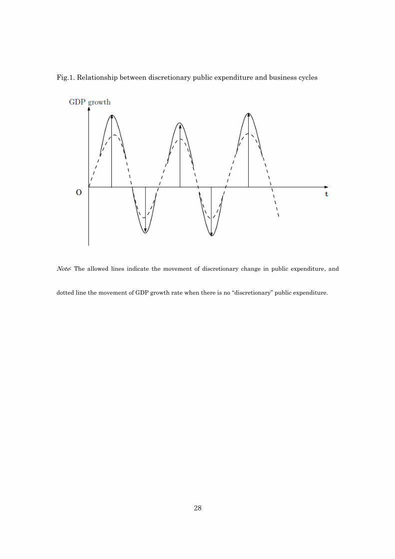
Fatás and Mihov (2003) show that this “discretionary changes” generate significant
economic fluctuations because they move procyclically as shown in Figure 1. This means
that the policy responses unrelated to the current economic conditions do amplify
business cycle fluctuations as the arrows in Figure 1 indicate. If this argument is true of
the regional economy and local public investment, some local public investment decided
by political factors would amplify regional business cycle fluctuations.
Section 2 explains an relationship between intergovernmental fiscal relations and
macro stabilization policy in Japan. Section 3 presents the empirical framework
underlying this research. Section 4 reports the estimation results and shows the
possibility that the local public investment decided by political factors may amplify
2 This also follows the explanation of Tang and Leung (2016). For more details, please see the page 18
on Tang and Leung (2016).

6
business cycles in a region. Section 5 concludes.
2. Local public investment and macro stabilization policy and in Japan
There are two types of projects in local public investment: the project subsidized by the
central government and local governments’ own project. Subsidized projects are
implemented using the national treasury disbursements, which is very little room for
local government on how to use. Local government’s own project is financed by local
government’s own tax revenues, local government bonds, and local allocation tax grants,
which are the intergovernmental transfers that local governments can use as they like.
Moreover, the issuance of local government bonds are repaid with local allocation tax
grants in the future.3
Table 1 shows the fiscal stimulus packages in Japan in the 1990s. According to this
table, public investment (public works excluding acquisition of land for public use) has
been often included in economic stimulus packages in Japan. Note that public works by
local government was also included in stimulus packages planned in August 1992, April
and September 1993, February 1994, September 1995, and April 1998.
3 See Pascha and Robaschik (2001) and Doi and Ihori (2009).

7
Economic stimulus packages include local public investments, regardless of whether
these investments are financially supported by the central government. The reason why
local governments in Japan have been involved in stabilization efforts by the central
government through their investment is that local governments have implemented
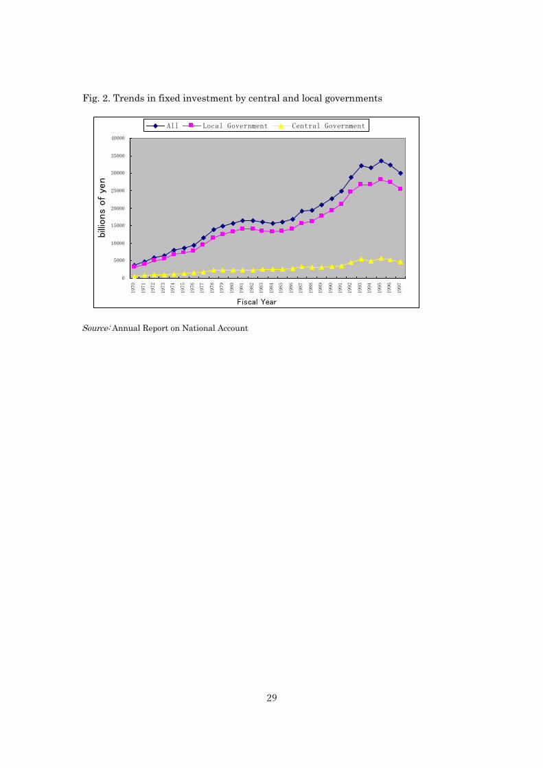
most public works. Figure 2 depicts the trends in fixed investment for the central
government and local governments. As shown, almost 80% of general government fixed
investment is implemented by local governments.
3 Empirical framework
3.1 Extraction of factors unrelated to current economic conditions
To clarify discretionary changes in local public investment expenditure, we apply the
following equation:
𝑙𝑜𝑔𝐿𝐺𝐼𝑖𝑡 = 𝛼𝑖 + 𝛽𝑡 + 𝛾𝑖𝑙𝑜𝑔𝑌𝑖𝑡 + 𝛿𝑖𝑙𝑜𝑔𝐿𝐺𝐼𝑖𝑡−1 + 휀𝑖𝑡 (1)
where i and t are prefecture and year indices, respectively. 𝛽𝑡 is a set of year dummies,
which captures the aggregate (country-level) economic conditions. 𝑙𝑜𝑔𝐿𝐺𝐼𝑖𝑡 is the

8
logarithm of real public investment by the local public sector (or ordinary construction
expenses of prefectures).4 𝑙𝑜𝑔𝑌𝑖𝑡 is the logarithm of real prefectural GDP (RGDP). This
is used as an independent variable that captures the “legitimate” changes in
expenditure. These specifications follow Fatás and Mihov (2003). 휀𝑖𝑡 is an error term.
We calculate volatility as the standard deviation of it̂ and denote it as 𝜎𝑖𝜀 , a
discretionary change in public investment expenditure.
Equation (1) contains a one-period lagged value of 𝑙𝑜𝑔𝐿𝐺𝐼𝑖𝑡. The lagged value of the
dependent variable is set as one period, following the specification of Fatás and Mihov
(2003). We estimate Equation (1) by taking first-difference and using dynamic panel
estimation developed by Arellano and Bond (1991). To avoid the problem of too many
instruments (Okui (2009) and Roodman (2009)), we assume the possible lagged values
of instrumental variables as at most two periods. Here the instruments are 𝑙𝑜𝑔𝐿𝐺𝐼𝑖𝑡−2,
𝑙𝑜𝑔𝐿𝐺𝐼𝑖𝑡−3, two valid lags of 𝑙𝑜𝑔𝑌𝑖𝑡, and year dummy variables.
4 It is also possible to analyze these two types of projects: local government’s own project and the one
subsidized by the central government as argued in Section 2. However, some papers like Kondoh
(2008) report that local governments tend to use these projects as substitutes depending on
availability of funds provided by the central government. In this case, it is not valid to analyze
separately because proportion of each expense in each year is affected by subsidy and it possibly leads
to imprecise estimates of 𝜎𝑖𝜀.

9
3.2 Effects on output volatility
To examine the link between discretionary local public investment and output
volatility, we estimate the effect of 𝜎𝑖𝜀 on the volatility of RGDP. The volatility of RGDP
is the standard deviation of the RGDP growth rate for each prefecture, 𝜎𝑖∆𝑌. The basic
specification is as follows:
𝑙𝑜𝑔𝜎𝑖∆𝑌 = 𝑐𝑜𝑛𝑠𝑡. +�̃�𝑙𝑜𝑔𝜎𝑖
𝜀 + 𝛽𝑙𝑜𝑔𝑋𝑖 + 𝑣𝑖 (2)
where 𝑋𝑖 is the independent variable other than 𝜎𝑖𝜀 that affects the volatility of RGDP,
and 𝑣𝑖 is the error term. Equation (2) is estimated using the residuals of Equation (1)
and the standard deviation of the RGDP growth rate. Therefore, when we estimate
Equation (2), independent variables other than 𝜎𝑖𝜀 are “averages” over the full sample
and we conduct a cross-section estimation following Fatás and Mihov (2003).
For 𝑋𝑖, we first use the ratio of government expenditure (the sum of government
capital formation and government consumption) to RGDP as the size of each region's
government. We do so because the volatility of RGDP may increase as the size of the
regional government increases.
Incidentally, economic fluctuations will increase with an increase in the proportion of

10
manufacturing and construction industries, respectively. To capture this effect, we add
the yearly output of manufacturing industries as a percentage of RGDP and that of
construction industries per RGDP. As fluctuations may vary according to the
characteristics of the industries. To address this issue, we use the specialization index
calculated followed by Krugman (1991) as in Fatás and Mihov (2001). In addition to 𝜎𝑖𝜀
and government size, these three variables related to industrial activities in a region
are used for our basic specification (Case 1, in Section 4). Furthermore, per capita
RGDP is added because economic fluctuations may increase in low-income regions.
Since economic linkages between different regions may affect the economic volatility
even in intranational studies, trade (sum of exports and imports, per RGDP) is also
considered. These follow Fatás and Mihov (2003) for Case 2 in our estimation model.
�̃� is expected to be both positive and negative. If it is estimated to be positive,
𝜎𝑖∆𝑌 increases the amplitude of fluctuations in the business cycle. That is, discretionary
changes in public investment cause the regional economy to fluctuate substantially.
Conversely, if this coefficient is estimated to be negative, the discretionary policy may
smooth regional business cycle fluctuations. The size of the government, proportion of
manufacturing industries, and trade are expected to be positive, and per capita RGDP is
expected to be negative. The coefficient of the specialization index is estimated to be

11
both positive and negative.
3.3. Determinants of discretionary factor and choice of instrumental variables
In Equation (2), the variation in 𝜎𝑖𝜀 may be more or less affected by output volatility.
Further, the government's size may be large during recessions and small during better
times. Therefore, the possible endogeneity of these two variables is addressed by using
instrumental variables. In contrast, however, to avoid the apprehension that the
instruments themselves are driven by output volatility, we should select variables
linked to the decision of the size of public investment expenditure and government size
in each region but unrelated to economic volatility.
Following the arguments in Section 1, we attribute the source of 𝜎𝑖𝜀 to political factors.
Using econometric approaches, Kondoh (2008) and Mizutani and Tanaka (2010) clarify
that the size of the public investment in each region of Japan has been affected by local
interest groups using econometric approaches. Further, the influence of median voters
within a region cannot be neglected. Needless to say, these affect the government size as
well as some local government investment decided by political factors, 𝜎𝑖𝜀.
Moreover, as far as the central government decides the size of the intergovernmental
transfers, which are used for financing most part of local government expenditure, local
12
government budgetary conditions may also be related to the government size and
politically motivated local government investment.
Following these, we select the instrumental variables summarized in Table 2.
First, we can employ variables that identify the influence of local interest groups as
one of the instruments. As proxies for interest groups' influence on public investment,
we use the average ratio of construction workers to all workers and the ratio of workers
in primary industries to all workers as in the case of Kondoh (2008), Mizutani and
Tanaka (2010), and Miyazaki (2016).
Incidentally, employment is very sensitive to the business cycle. To deal with this, we
exclude the cyclical factors from the actual data by using the time trend estimation
approach proposed by Hodrick and Prescott (1997). We do so for the number of the
workers in each prefecture, the number of workers in construction industries, and the
number of workers in primary industries.
We name the potential value of these as the ratio of “potential” construction workers to
all “potential” workers and the ratio of “potential” workers in primary industries to all
“potential” workers. Thus, we ensure that these two variables are uncorrelated with
economic volatility, but remain strongly related to the “discretionary” part of public
investment and government size following the arguments shown in the former

13
paragraph. Thus, we can use these in conducting a 2SLS estimation.
Second, to capture the median voter's influence, we use the average of the median
income. Finally, budgetary conditions in each prefectural government also decide the
size of local government’s investment. For budgetary conditions, we employ the average
ratio of the outstanding prefectural government debt.
4. Empirical results
Our annual panel covers the period 1990-2007 for 47 Japanese prefectures. We begin
our sample period after the 1990s because the Cabinet Office of Japan does not provide
data before the 1990s on the basis of the System of Integrated Environment and
Economic Accounting proposed by the United Nations in 1993 (SNA93 data).As a result,
we have no other choice but to set the sample period after 1990.5
Moreover, although we obtain the data for 1990-2003 in real terms by using the 1995
deflator, we cannot acquire real-term data using the 1995 deflator for 2004-2007.
5 The Cabinet Office of Japan conducts retrospective estimation on the RGDP and related data of the
1980s (http://www5.cao.go.jp/keizai3/database.html ). Here the adjustment factor is used for
retrospective estimation. However, since the empirical results may differ depending on the adjustment
factor, it seems unfavorable to use all of this data in empirical estimations. Another option is to use
SNA68 data, following Artis and Okubo (2011) and Brückner and Tuladhar (2013). However, it is
desirable to use the data made by using the new method to the extent possible. Therefore, we use SNA
93 data.

14
Therefore, we must construct the real data for 2004-2007 by the 1995 deflator.6
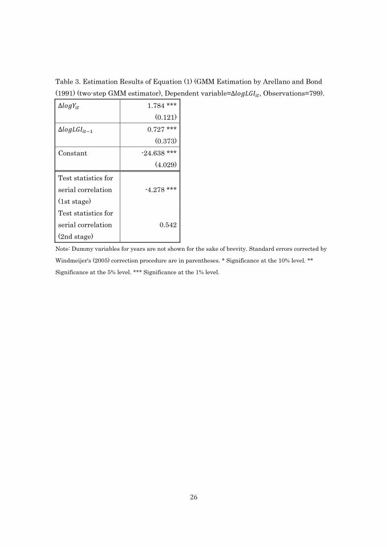
First, we present the results of equation (1) in Table 3. Before presenting the results,
we determine that there is no second-order serial correlation for the disturbances in the
first difference equation. This test is important because the consistency of the GMM
estimator relies on no autocorrelation between the disturbance of period t and period t-1.
According to the results shown in the table, we can confirm that there is no serial
correlation between ∆𝑣𝑖𝑡 and ∆𝑣𝑖𝑡−2. The lagged value of the dependent variable is set
as one period.7 The result shows that the coefficients of ∆𝑙𝑜𝑔𝑌𝑖𝑡 and ∆𝑙𝑜𝑔𝐿𝐺𝐼𝑖𝑡−1 are
positive and significant.
We present the results of Equation (2) in Table 4. Before we present the estimation
results for the coefficients, we first confirm the correlation between two endogenous
variables, 𝜎𝑖𝜀 and government size, and the instrumental variables in the 2SLS
estimation. The results show that correlations between 𝜎𝑖𝜀 and the instrumental
variables are strong. Second, we determine the validity of the instrumental variables.
The results of the Sargan test indicate that the null cannot be rejected for all cases.
These results validate our choice of instrumental variables.
Although we conduct a cross-section estimation for Equation (2), our samples are very
6 Appendix offers further details concerning this point and the source of the data. 7 Since we correct the bias in the two step standard errors by the Windmeijer's (2005) correction
procedure, please pay attention that we do not perform over-identification restriction test.
15
small because the sample size is at most 47. Moreover, since the volatility of unexpected
local public investment is estimated in the first estimation equation, a problem of
generated regressor is a concern. To deal with these, we calculate the standard error by
150 bootstrap replications.
The coefficient of 𝜎𝑖𝜀 is estimated to be positive and significant in Case 1. However,
the results become insignificant when we add trade and per capita RGDP in Case 2.
While the coefficient of government size is not estimated to be significant, the
proportion of manufacturing industries is estimated to be positive and significant for
both cases. The results show that the volatility of regional economies increases with an
increase in the proportion of manufacturing industries.
5. Conclusion
This paper examines the relationship between local public expenditure and business
cycle fluctuations of Japanese prefectures, with a focus on public investment. Our
empirical results show that “discretionary changes” in local public investment, that is,
the part of investment decided by political factors, does not necessarily amplify the
fluctuations in prefectural business cycles for all cases. This may be caused by the

16
characteristics of local public investment. Most local public investments are related to
improving the living environment such as housing, education facilities, and sanitation
and health, etc. Public investments related to improving the living environment may
directly replace private consumption or investment from their characteristics. Miyazaki
(2009) shows that local public investment does not have a positive impact on the
business cycles using macro-monthly data, and attributes the reason for this to the
direct crowding-out effects caused by the characteristics of local public investment.
Since this may be true of the regional economy and local public investment may not
necessarily have a positive impact on the regional economy, we cannot show robust
results for 𝜎𝑖𝜀 on the economic volatility.
On the other hand, relations with economic growth may also be considered, as in the
case in Ramey and Ramey (1995), Fatás and Mihov (2001), and Fatás and Mihov (2003).
This point should be considered in future research.
Acknowledgement
We thank for Kazumi Asako, Ryokichi Chida, Yutaka Harada, Makoto Hasegawa,
Masayoshi Hayashi, Bernd Hayo, Kazuki Hiraga, Yasushi Iwamoto, Masumi Kawade,

17
Hideki Kohishi, Hiroki Kondo, Takeshi Miyazaki, Junichi Nakamura, Florian
Neumeuer, Hiroki Tanaka, Yasuhiro Tsukahara, Atsuko Ueda, Tomoaki Yamada, the
participants in the seminar at Doshisha University, Meiji University, Hitotsubashi
University, University of Marburg, UC Irvine, and Waseda University for insightful
comments and suggestions. This work has been financially supported by the Japan
Society for the Promotion of Science (Grant-in-Aid for Scientific Research # 26380361).
The usual disclaimer applies.
Appendix
Data for prefectural GDP, manufacturing output, construction output, exports,
imports, government capital formation, and government consumption in each
prefecture came from the Annual Report on Prefectural Accounts by the Cabinet Office
in Japan.8
The 1990-2003 data are expressed in real terms by using 1995 as the deflator. Since we
were unable to acquire real-term data by using the 1995 deflator for 2004-2007, we
8 For Aichi Prefecture, the exports and imports expressed in real terms are not from the Annual
Report on Prefectural Accounts. These variables are downloaded from the official website of the Aichi
prefectural government. Incidentally, to express in real terms, we use the deflator of PGDP because we
cannot acquire the deflator of exports and imports of Aichi.

18
constructed real term 2004 data by using the 1995 deflator as follows:
𝑌𝑖,2004∗ = 𝑌𝑖,2003 + 𝑌𝑖,2003 ∗ 𝑔𝑖,2004−2003
∗ , (A.1)
where 𝑌𝑖,2004∗ is 2004 data expressed in real terms using the 1995 deflator, and 𝑌𝑖,2003 is
2003 data expressed in real terms using the 1995 deflator, and 𝑔𝑖,2004−2003∗ is the real
growth rate of variable Y over the period 2003-2004 (using the 2000 deflator). We also
constructed the 2005-2007 real data using the 1995 deflator, following the procedure
above.
Data on the local government investment is the ordinary construction of each
prefecture from the Annual Statistics of Local Public Finance by the Ministry of
Internal Affairs and Communications (hereafter MIAC). Incidentally, we cannot acquire
the data in real terms in this data. We can acquire the deflator from 1990 to 2003 by the
deflator of 1995. After 2003, we construct the 2004 deflator from the 1995 deflator as
follows:
𝑃𝑖,2004∗ = 𝑃𝑖,2003 +△ 𝑃𝑖,2004−2003
∗ , (A.2)

19
where 𝑃𝑖,2004∗ is the 2004 deflator by the 1995 deflator, 𝑃𝑖,2003 is the 2003 deflator by
the 1995 deflator, and △ 𝑃𝑖,2004−2003∗ is the change over 2003-2004 of the PGDP deflator
in the 2000 deflator. We acquire the deflator for 2005-2007 by using the 1995 deflator,
following the procedure above. By using these deflators, the ordinary construction of
each prefecture is expressed in real terms.
The index of specialization is based on Fatás and Mihov (2001), following Krugman
(1991). Let 𝑠𝑗𝑖 be the share of Industry j in Prefecture i, we measure specialization as
𝑆𝑃𝐸𝐶𝑖 = ∑ |𝑠𝑗𝑖 − 𝑠𝑗,𝐴|𝐼𝑗=1 (A.3)
where 𝑠𝑗,𝐴 represents the share of Industry j in Japan as a whole. There are eleven
comparable sectors.9 All of the data are from Annual Report on Prefectural Accounts by
the Cabinet Office in Japan.
Median income is relative median income. This is the ratio of the median income to the
mean income. The “median” and “mean” incomes are calculated from tables on the
income distribution of households reported in the “Basic Survey on Employment
9 These are the agriculture, forestry and fisheries industry, the mining industry, the manufacturing
industry, the construction industry, utilities, the wholesale trade industry, the finance and insurance
industry, the real estate industry, the transportation and communications industry, and the service
industry.

20
Structure” by the MIAC. This is the data that Kondoh (2008) used for estimation.10
Data on outstanding local government bonds are from the annual statistical reports by
MIAC. This is expressed in real terms by the deflator that we indicated before.
The ratios of workers in the primary and construction industries were determined by
dividing the number of workers in these industries by the total number of workers.
These data come from the Labor Force Survey of the Ministry of Internal Affairs and
Communications (MIAC). The Labor Force Survey data can be obtained for 1990, 1992,
1995, 1997, 2000, 2002, 2005, and 2007. To perform the time trend estimation, we
interpolate using the growth rate. For example, we obtain the data for 1991 as follows:
𝑁𝑖,1991∗ = 𝑁𝑖,1990 +
𝑁𝑖,1992−1990
2, (A-4)
where 𝑁𝑖,1991∗ denotes 1991 labor data, 𝑁𝑖,1990denotes 1990 labor data, and
𝑁𝑖,1992−1990
2
denotes the change in labor over 1990-1992. Likewise, we acquire the data for 1996,
2001, and 2006. Further, we obtain the data for 1993 as follows:
𝑁𝑖,1993∗ = 𝑁𝑖,1992 +
𝑁𝑖,1995−1992
3, (A-5)
10 This is the average of 1993, 1998, and 2003 because these three years’ data are available during our
sample periods.

21
where 𝑁𝑖,1993∗ denotes 1993 labor data, 𝑁𝑖,1992 denotes 1992 labor data, and
𝑁𝑖,1995−1992
3 denotes the change in labor over 1992-1995. Similarly, we obtain the data for
1994, 1998, 1999, 2003, and 2004.
References
Arellano, M., Bond, S., 1991. Some tests of specification for panel data: Monte Carlo
evidence and application to employment equation. Review of Economic Studies 58 (2),
pp.277-297.
Artis, M., Okubo, T., 2011. The intranational business cycle in Japan. Oxford Economic
Papers 63 (1), pp.111-133.
Brückner, M., Tuladhar, A., 2014. Local government spending multipliers and financial
distress: Evidence from Japanese Prefectures. The Economic Journal, 124 (581),
pp.1279-1316.
Doi, T., Ihori, T., 2009. The Public Sector in Japan. Edward Elgar Publishing,
Chelthenham, UK.
Fatás, A., Mihov I., 2001. Government size and automatic stabilizers: International and
intranational evidence. Journal of International Economics 55, pp.3-28.

22
Fatás, A., Mihov I., 2003. The case for restricting fiscal policy discretion. Quarterly
Journal of Economics 118 (4), pp.1419-1447.
Funashima, Y., 2014. Macroeconomic policy coordination between Japanese central and
localgovernments. Papers presented at the 2014's Autumn meeting of Japanese
Economic Association.
Funashima, Y., Horiba, I., Miyahara, K., 2015. Local government investment and
ineffectiveness of fiscal stimulus during Japan's lost decades. MPRA Paper No. 61333.
Hodrick, R. J., Prescott, E. C., 1997. Post-war U.S. business cycles: An empirical
investigation. Journal of Money, Credit and Banking 29 (1), pp.1-16.
Kondoh, H., 2008. Political economy of public capital formation in Japan. Public Policy
Review 4 (1), pp.77-110.
Krugman, P., 1991. Geography and Trade. MIT Press, Cambridge.
Miyazaki, T., 2009. Public investment and business cycles: The case of Japan. Journal
of Asian Economics 20 (4), pp.419-426.
Miyazaki, T., 2010. Local public sector investment and stabilization policy: Evidence
from Japan. Public Policy Review 6 (1), pp.153-166.
Miyazaki, T., 2016. Public investment and regional business cycle fluctuation in Japan.
Applied Economics Letters, forthcoming.

23
Mizutani, F., Tanaka, T., 2010. Productivity effects and determinants of public
infrastructure investment. The Annals of Regional Science 44 (3), pp. 493-521.
Mochida, N., 2008. Fiscal Decentralization and Local Public Finance in Japan. New
York, Routledge.
Okui, R., 2009. The optimal choice of moments in dynamic panel models. Journal of
Econometrics 151, pp.1-16.
Pascha, W., Robaschik, F., 2001. The role of Japanese local governments in stabilization
policy. Duisburg Working Papers on East Asian Studies 40, University of
Duisburg-Essen.
Roodman, D., 2009. A note on the theme of too many instruments. Oxford Bulletin of
Economics and Statistics 71 (1), pp.135-58.
Stoney C., Krawchenko, T., 2011. Transparency and accountability in infrastructure
stimulus spending: A comparison of Canadian, Australian and US programs. Papers
presented at Canadian Political Science Association Annual Conference.
Tang, S. H. K., Leung, C. K. Y., 2016. The deep historical roots of macroeconomic
volatility. Economic Record, forthcoming.
Windmeijer, F., 2005. A finite sample correction for the variance of linear efficient
two-step GMM estimators. Journal of Econometrics 126 (1), pp.25-5

24
Table 1. Fiscal Stimulus Packages in the 1990s (JPY trillion)
Note: This table is followed by Brückner and Tuladhar (2014). Other government investment
comprises investment in fields such as science and technology, education and social welfare,
alternative energy and environment, and natural disaster relief. All government investment in the
economic stimulus packages in April 1995 comprised natural disaster relief because this package was
planned as a countermeasure against the Great Hanshin-Awaji Earthquake.

25
Table 2. Endogenous variables and instrumental variables used in 2SLS estimation.
Endogenous variables Instruments
1. "Discretionary" part
of the investment (𝜎𝑖𝜀)
I. Average of prefecture’s
government debt outstanding
2. Government size
(The average of
government
expenditure/RGDP)
II. Average of the median income
of each prefecture
III. Average of the ratio of
potential construction workers to
all potential workers
IV. Average of the ratio of
potential workers in primary
industries to all potential
workers
26
Table 3. Estimation Results of Equation (1) (GMM Estimation by Arellano and Bond
(1991) (two-step GMM estimator), Dependent variable=∆𝑙𝑜𝑔𝐿𝐺𝐼𝑖𝑡, Observations=799).
∆𝑙𝑜𝑔𝑌𝑖𝑡 1.784 ***
(0.121)
∆𝑙𝑜𝑔𝐿𝐺𝐼𝑖𝑡−1 0.727 ***
(0.373)
Constant -24.638 ***
(4.029)
Test statistics for
serial correlation
(1st stage)
-4.278 ***
Test statistics for
serial correlation
(2nd stage)
0.542
Note: Dummy variables for years are not shown for the sake of brevity. Standard errors corrected by
Windmeijer's (2005) correction procedure are in parentheses. * Significance at the 10% level. **
Significance at the 5% level. *** Significance at the 1% level.

27
Table 4. Estimation Results of Equation (2) by 2SLS Estimation (Dependent variable=
𝑙𝑜𝑔𝜎𝑖∆𝑌, Observations=47)
Case1 Case2
𝜎𝑖𝜀 0.527 * 0.530
(0.282) (0.349)
Government
expenditure/RGDP 0.384 * 0.683
(0.250) (0.544)
Specialization
index 0.181 0.179
(0.116) (0.125)
Share of
manufacturing
industries/RGDP
0.520 *** 0.517 *
(0.134) (0.319)
Share of
construction
industries/RGDP
-0.232 -0.268
(0.362) (0.495)
Per capita RGDP
0.105
(0.559)
Trade
0.021
(0.419)
Constant -1.911 *** -2.019
(0.726) (1.290)
𝑅2 0.257 0.240
Partial F-statistics
for 𝜎𝑖𝜀
2.41 * 3.24 **
Partial F-statistics
for government
expenditure/RGDP
16.49 *** 7.52 ***
Sargan statistics 0.555 (2) 0.548 (2)
Note: We take the logarithm of all independent variables (the average of sample periods except
𝜎𝑖𝜀) in
estimation. The standard errors with 150 bootstrap replications are in parentheses. The Sargan
statistics are chi-square statistics for the overidentification restriction test with the degree of freedom
shown in parentheses. * Significance at the 10% level. ** Significance at the 5% level. *** Significance
at the 1% level.
28
Fig.1. Relationship between discretionary public expenditure and business cycles
Note: The allowed lines indicate the movement of discretionary change in public expenditure, and
dotted line the movement of GDP growth rate when there is no “discretionary” public expenditure.
29
Fig. 2. Trends in fixed investment by central and local governments
Source: Annual Report on National Account
0
5000
10000
15000
20000
25000
30000
35000
400001970
1971
1972
1973
1974
1975
1976
1977
1978
1979
1980
1981
1982
1983
1984
1985
1986
1987
1988
1989
1990
1991
1992
1993
1994
1995
1996
1997
Fiscal Year
billions
of
yen
All Local Government Central Government
Top Related