


Languages
Pages
Legal


University of South Florida University of South Florida
Scholar Commons Scholar Commons
Graduate Theses and Dissertations Graduate School
2005
Light Element and Lithium Isotope Signatures of the EMII Light Element and Lithium Isotope Signatures of the EMII
Reservoir - The Society Islands, French Polynesia: Geochemical Reservoir - The Society Islands, French Polynesia: Geochemical
Results and an Educational Application Results and an Educational Application
Judy Ann Harden University of South Florida
Follow this and additional works at: https://scholarcommons.usf.edu/etd
Part of the American Studies Commons
Scholar Commons Citation Scholar Commons Citation Harden, Judy Ann, "Light Element and Lithium Isotope Signatures of the EMII Reservoir - The Society Islands, French Polynesia: Geochemical Results and an Educational Application" (2005). Graduate Theses and Dissertations. https://scholarcommons.usf.edu/etd/2914
This Thesis is brought to you for free and open access by the Graduate School at Scholar Commons. It has been accepted for inclusion in Graduate Theses and Dissertations by an authorized administrator of Scholar Commons. For more information, please contact [email protected].

Light Element and Lithium Isotope Signatures of the EMII Reservoir - The Society
Islands, French Polynesia: Geochemical Results and an Educational Application
by
Judy Ann Harden
A thesis submitted in partial fulfillment of the requirements for the degree of
Master of Science Department of Geology
College of Arts and Sciences University of South Florida
Co-Major Professor: Jeffrey G. Ryan, Ph.D. Co-Major Professor: H. Leonard Vacher, Ph.D.
Charles B. Connor, Ph.D.
Date of Approval: March 24, 2005
Keywords: Boron, geochemistry, mantle, ocean island basalts, quantitative literacy
© Copyright 2005, Judy Ann Harden

Dedication
I would like to dedicate this thesis to a husband and children who constantly
encouraged and supported me, to parents who instilled a love for travel and a fascination
for rocks and volcanoes, to the professors at Hillsborough Community College that
helped launch my dreams, and to the faculty and staff at the University of South Florida
who helped make those dreams come true.
Acknowledgments
I would like to thank Dr. Jeff Ryan and Dr. Len Vacher for guiding, training, and
teaching me and putting up with my continual harassment while working on this thesis
and Dr. Connor for his insight, encouragement, and support. I also want to thank Dr.
Ivan Savov and Dr. Rob Watts who so freely shared their knowledge, companionship,
time, and encouragement. I owe a great deal to the wonderful staff of the Gump
Research Station who made me feel so welcome. A special thank you goes to Dr.
William White who donated samples from his personal collection for other islands in the
Society Chain; although, I probably missed out on a really nice trip due to his generosity.
I would also be amiss if I neglected to thank Professor Henry Aruffo for encouraging me
to take his “Geography of Tahiti and Moorea class” and sharing his love for an island and
its people with so many students.

i
Table of Contents
List of Tables iv
List of Figures v
Abstract vii
Prologue ix
Part I - B, Be, Li and Li isotopic systematics of the Society Islands: Insights into the nature of EMII Mantle sources 1 Introduction 1
Geologic Setting 5
Age/Plate Movement 6
Volcanism 7
Eruptive Products and Lava Composition 9
Previous Work 10
Mantle Plumes and Hotspot Volcanism 10
Geochemistry of Hotspot Volcanics 12
Previous Work on B, Be, Li in Ocean Islands 13
Sampling and Analysis 17
Sample Collection 17
Petrology/Petrography 18

ii
Geochemical Methods 23
Major and Trace Elements 23
Light Elements 23
Lithium Isotopes 24
Results 26
Major Element Variations 26
Trace Elements 27
B-Be-Li Concentrations 28
Li Isotopes 33
Discussion and Conclusions 35
Part II – Instructional Modules 39
Introduction 39
Module JAH1A & JAH1B – Fractional Crystallization 43
Module JAH2A & JAH2B – Partial Melting 46
Evaluation of Fractional Crystallization Modules 48
Comments on Evaluation Design 51
Results 53
Conclusions 54
References 55
Appendix I 65
Appendix II 68
Fractional Crystallization Module JAH1A 68

iii
Fractional Crystallization Module JAH1B 77
Partial Melting Module JAH2A 86
Partial Melting Module JAH2B 92

iv
List of Tables
Table 1. Major and trace element data from senior thesis (Harden, 2002) for Moorea samples collected in 2001 65
Table 2. Major and trace element data for Moorea samples collected in 2003. 66 Table 3. Li, Be, and B analysis for 20 samples from Moorea and 13 samples
from other Society Islands as indicated. 67 Table 4. δ7Li values for 6 samples from Moorea and 6 samples from other
Society Islands. 67

v
List of Figures
Figure 1. Location map showing study area of Society Islands, French Polynesia. 5
Figure 2. Society Island positions, age, and distance from hot spot (after Maury, 2000). 7
Figure 3. Effusive lava flows from Pu`u O`o crater, Kilauea, Hawaii
representative of most eruptions at an ocean island hot spot (photo taken March, 2003). 8
Figure 4. Total Alkali-Silica classification of volcanic rocks collected from the
island of Moorea.. 9 Figure 5. Island of Moorea with sample collection sites (red dots) and sample
names. 17 Figure 6. Primitive basalt (M01Fish2D) with subhedral olivine and euhedral
pyroxene with reaction rim phenocrysts. 18 Figure 7. M01 B2B hawaiite in plain & crossed-polarized light, plagioclase
microphenocrysts with euhedral olivine glomerocryst intergrowth (40X). 19
Figure 8. M01 PK 25N Benmoreite with trachytic texture (plagioclase, spinel,
pyroxene microphenocrysts) (40X). 20 Figure 9. Pyroxenite xenolith on left, right side is groundmass with
microphenocrysts of plagioclase, olivine, and pyroxene, plain & crossed-polarized (40X). 21
Figure 10. All samples plot within Alkalic field (Modified from Macdonald &
Katsura, 1964). 26 Figure 11. TiO2 contents increase with decreasing MgO. At ~5% Magnesium,
Titanium decreases sharply indicating the crystallization of magnetite in the magma chamber. 27
Figure 12. Samples from Moorea follow predicted model for fractional
crystallization for a range of F from 1.0-0.5. 28

vi
Figure 13. Li vs MgO (a) and Be vs MgO (b) contents for Moorea (turquoise squares), and Society Islands (navy squares) with similar trajectories suggestive of similar parental source. 29
Figure 14. B/Be ratios range from 0.6-2.0. 31 Figure 15. B/K2O ratios range from 0.7-2.0 32 Figure 16. Society samples fall within a range of values for δ7Li similar to those
of MORBs, Erebus, and other OIBs. 33 Figure 17. Society samples fall within the upper values of Nishio et al., (2004)
data for the EMI reservoir and the serpentinites of Benton et al., (2004) but do not exhibit any range variation. 34
Figure 18. A) Basalts erupted at the Society Island plume are alkalic in
composition due to lower temperatures, higher pressure, and/or smaller degree of partial melting. 37
Figure 19. Results of questions posed to students both pre- and post-lecture
regarding the process of fractional crystallization. 53

vii
Light Element and Lithium Isotope Signatures of the EMII Reservoir - the Society Islands, French Polynesia: Geochemical Results and an Educational Application
Judy Ann Harden
ABSTRACT
The purpose of this thesis is to examine the abundance systematics of Li, Be and
B, and Li isotopic systematics in lavas from the Society Islands, an enriched mantle
(EMII) intraplate site, to further characterize the chemical signatures in the sources for
ocean island basalts that may result from subduction-related processes and mantle
entrainment. The goal is to see how light-element and Li-isotope systematics vary during
ocean-island volcanic evolution and during tropical weathering.
B/K, B/Be and Li/V ratios in basaltic Moorea lavas are 0.0001-.0002, 0.6-2.0 and
0.01-0.05 respectively, and the more evolved samples are somewhat higher. These ratios
are similar to those for other Society Island lavas, and lower than those for lavas from St.
Helena, Erebus, Hawaii, Gough and Reunion, as well as analyzed mid-ocean ridge basalts
(MORBs). δ7Li values for Moorea cluster at +3 ─ +5‰ for the freshest lavas, and 0 ─
+2‰ for more weathered rocks.
These new data from Moorea are consistent with earlier survey results from the
Society Islands and indicate a mantle source that includes B-poor (subducted?) materials.
δ7Li values for the freshest Moorea samples are similar to those of other Society Island
lavas, suggesting that the EMII isotopic end-member records a Li-isotopic signature

viii
similar to that of MORBs. Dilution by entrainment of upper mantle material is unlikely
due to differing B/K ratios and similar δ7Li values for the Society and Hawaiian plumes.
A more likely explanation is that recycled crust or sediments have minimal influence on
the Li isotope signatures of hotspot plumes.
Using the Moorea data and geochemical data from other sources, I created a set of
Power Point instructional modules for use in petrology classes to aid in teaching students
about the effects of fractional crystallization and partial melting. I tested the module on
fractional crystallization in two upper-level geology classes to assess its value in
increasing student understanding. Both classes received a lecture about fractional
crystallization. One class worked through the module as a homework exercise, while the
other did not use the module. Students who worked through the module in addition to the
lecture showed an increased understanding of the concept of fractional crystallization.
ix
Prologue
This thesis consists of two parts. The first section is a geochemical examination
of ocean island basalts from the island of Moorea, French Polynesia, and other islands of
the Society Islands chain. The second part uses this collected data to produce a set of
instructional modules for use in classrooms to further student understanding of processes
of fractional crystallization and partial melting in the Earth’s mantle.

1
PART I
B, Be, Li and Li isotopic systematics of the Society Islands: Insights into the nature
of EMII Mantle sources
Introduction
Radiogenic isotope ratios have been used for the past 40 years to answer
questions about processes within the Earth’s interior. Questions posed by Hart (1988),
Hofmann (1988) and others include: How many discrete geochemical domains exist in
the mantle? How do these domains form? Where are they located within the Earth?
The deep mantle plumes responsible for the generation of ocean island basalts
globally have been characterized in terms of four main “end- members” defined by Pb,
Sr, and Nd, isotope signatures. DMM is the depleted mantle source for mid-ocean ridge
basalts (MORBs). HIMU mantle has elevated U/Pb ratios (µ), as indicated by high
206/204Pb and 207/204Pb. EMI is enriched mantle with very unradiogenic 206Pb/204Pb and the
lowest 143Nd/144Nd present in the oceans. EMII is enriched mantle and contains the
highest 87Sr/86Sr in the ocean and intermediate 206Pb/204Pb and 143Nd/144Nd (Hart, 1988).
Because radiogenic isotope ratios are not modified during partial melting and magma
chamber processes, data for lavas can be used to characterize the mantle source regions
of basaltic magmas.
The HIMU and the EM isotopic reservoirs have been attributed to subduction-
related origins in the past (Hofmann and White, 1982; Zindler and Hart, 1986; Hart,

2
1988; Hauri and Hart, 1993; Reisberg et al., 1993; Thirwall, 1997). However, such
inferences are not equivocal because the processes of subduction profoundly modify the
composition of slab materials as they descend into the mantle, invalidating comparisons
with the original surface materials (i.e. sediments and ocean crustal rocks) that are carried
into trenches (Bebout et al., 1993; 1999; Schmidt and Poli, 2003). Tracers are required
that are both sensitive to the process in question and well documented in terms of their
terrestrial distribution to confirm the role of subduction or any other terrestrial
geochemical process in creating a mantle domain.
The systematics of the light elements Li, Be, and B are well understood in
subduction-zone processes and are used to characterize volcanic rocks in all tectonic
settings (see Ryan and Langmuir, 1987; 1988; 1993; Ryan et al., 1996; Leeman and
Sisson, 1996; Ryan, 2002; Morris and Ryan, 2003; and references therein). Boron
systematics in intraplate lavas globally point to a substantial B depletion in these mantle
sources and boron isotopic ratios lower than those of MORBs (Ryan et al., 1996;
Chaussidon and Marty, 1995). In contrast, Be abundances in intraplate lavas are
markedly elevated (Ryan, 2002).
Recently the stable-isotope system of lithium (consisting of its two isotopes 6Li
and 7Li), expressed as per-mille variations of δ7Li from the value of the NIST standard
reference material L-SVEC (7Li/6Li = 12.01), has been used successfully to characterize a
variety of Earth reservoirs and processes (Chan et al., 1992, 1994, 1999; 2003; Tomascak
et al., 2000; 2002; Pistiner and Henderson, 2003; Rudnick and Nakamura, 2004). This
system is useful in studying geologic processes involving low- to moderate-temperature
fluid-rock exchanges because of the large mass difference between 6Li and 7Li (~17%)

3
(Tomascak et al., 1999) and the potentially large mass fractionations of the two Li
isotopes in nature (∂7Li oceans = +32.3‰; sediment up to + 20 ‰; mantle rocks: -17‰ to
+12‰, Chan and Edmond, 1988; Chan et al., 1992; Nishio et al., 2004, Rudnick and
Nakamura, 2004). The ongoing development of multi-collector inductively coupled
plasma-source mass spectrometry (ICP-MS) has facilitated the study of this isotopic
system, as it permits the relatively rapid determination of δ7Li values on large numbers of
samples.
Lithium isotopic compositions of lavas accurately represent their sources because
isotope fractionation does not appear to occur during high-temperature crystal-liquid
fractionation processes (Tomascak et al., 1999). Lithium isotopes have been used in
defining the role of subducted sediment (Chan et al., 1999; 2002), basaltic crust (MORB
or eclogites) (Chan et al., 2000; Tomascak et al., 2002; Zack et al., 2004; Bouman et al.,
2004), seawater, continental crust (Teng et al., 2004) and combinations of these in arc
magma sources.
As a step in more rigorously assessing the role of subduction in intraplate mantle
sources, I characterized a suite of samples from the island of Moorea, of the Society
Islands in French Polynesia, for their B, Be, Li abundances and Li-isotope signatures. I
also analyzed alkali basalts from the other Society Islands to define the overall light-
element signature of the Society chain and to see if temporal variations are evident. The
radiogenic-isotope signatures of these EMII-type, hotspot-derived lava suites preserve a
signature of past subduction (specifically a subducted sediment signature; White et al.,
1982, 1996). Because the behaviors of light elements during subduction are known in

4
great detail, we may be able to say with greater confidence that an enrichment or
depletion in B/Be or δ7Li in these lavas is related to a process that happened during an
ancient subduction event.
5
Geologic Setting
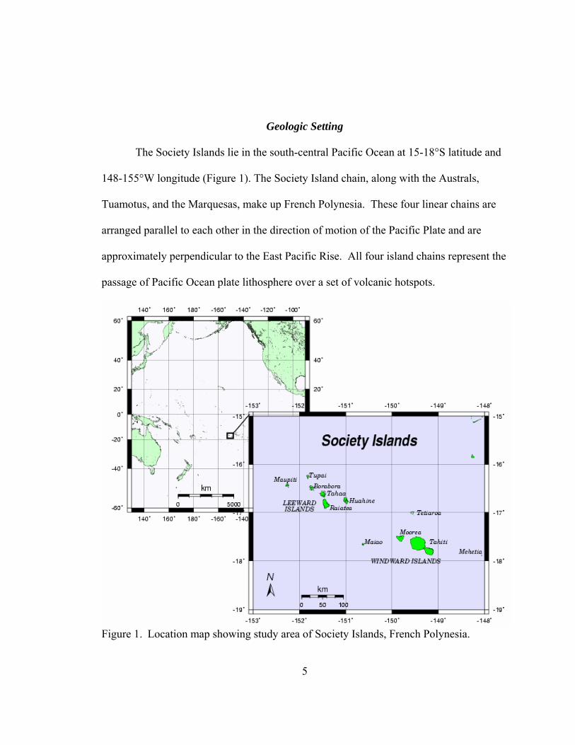
The Society Islands lie in the south-central Pacific Ocean at 15-18°S latitude and
148-155°W longitude (Figure 1). The Society Island chain, along with the Australs,
Tuamotus, and the Marquesas, make up French Polynesia. These four linear chains are
arranged parallel to each other in the direction of motion of the Pacific Plate and are
approximately perpendicular to the East Pacific Rise. All four island chains represent the
passage of Pacific Ocean plate lithosphere over a set of volcanic hotspots.
Figure 1. Location map showing study area of Society Islands, French Polynesia.
6
Islands, seamounts, and atolls comprise the Society Chain. The islands extend
over 700 km with the youngest island, Mehetia, lying to the southeast and the oldest
island, Maupiti, to the northwest. Radiometric dating shows that the islands of the
Society chain become progressively older to the northwest (4.5Ma – present; Okal,
1987). The land area of the Society Islands is 2,095 km2. Each island is highly dissected
and consists of a basaltic volcanic core that has undergone erosion and denudation
(Williams, 1933).
Geographically, the Society Islands form two groupings. Tahiti, Moorea, Maiao,
Mehetia and the atoll of Tetiaroa make up the Windward Islands. The older islands
Raiatea, Tahaa, Huahine, Borabora, Maupiti and the atoll of Motuiti constitute the
Leeward Islands.
Moorea is the second largest island in the Society chain, with an area of 132 km2
(Stearns, 1978). This island, like the others, represents the summit of a large, eroded,
alkali-basalt shield volcano that rises approximately 4,000 m from the ocean floor. Mt.
Tohiea, the highest peak of Moorea, has an elevation of 1,207 m (or ~5,200 m above the
ocean floor). The island includes a deeply eroded caldera, the northern rim of which has
largely collapsed, with only an isolated remnant preserved, Mt. Rotui. Two large bays,
Opunohu and Cook’s, on the north side of the island, give the island its tooth-shaped
appearance.
Age/Plate Movement
The volcanism of Moorea and the other Society Islands is classically intraplate in
nature. Samples collected by Dymond (1975) indicate an age of 1.65 ± 0.13 Ma for

7
Moorea and 0.65 ± 0.22 Ma for Tahiti. The difference in ages of these two islands
correlates with the proposed movement of the Pacific Plate (Figure 2) at 11 cm/yr over a
fixed hot spot or deep mantle plume (Dymond, 1975).
Figure 2. Society Island positions, age, and distance from hot spot (after Maury, 2000).
Volcanism
There is no historical record of volcanic activity for any of the Society Islands.
However, from March to December, 1981, Mehetia (the island over current hotspot)
experienced over 3,500 earthquakes associated with underwater eruptions at a depth of
1,600 m (Binard et al., 1993).
Until recently, the common assumption about Pacific hotspot volcanism was that
it is dominated by effusive basaltic lava flows (Figure 3) with occasional fire fountains.
Recent discoveries, however, indicate that explosive volcanism has occurred during the
formation of ocean islands. One such pyroclastic deposit near the top of Kulanaokuaiki
Pali covers approximately 450 km2 of the summit area of Kilauea (Fiske et al., 1999).

8
Figure 3. Effusive lava flows from Pu`u O`o crater, Kilauea, Hawaii representative of most eruptions at an ocean island hot spot (photo taken March, 2003).
With similar geochemistry, tectonic setting, and form, the possibility exists that
explosive volcanism did occur during the formation of the Society Islands. Neither the
rock record nor collected samples from Moorea, however, show evidence of explosive
volcanism. Evidence for explosive volcanism on Moorea may no longer exist due to the
much older age of this island and the amount of erosion that has taken place.
There is, however, a unit described as a thick, columnar pyroclastic formation on
the island of Tahiti, in the upper stage of its second shield. Eroded blocks from this unit,
sampled in the Vaitamanu River, constitute an ignimbrite facies (Hildenbrand, 2003).
Although most of the Society Islands probably formed by effusive volcanism, explosive
activity can no longer be ruled out.
9
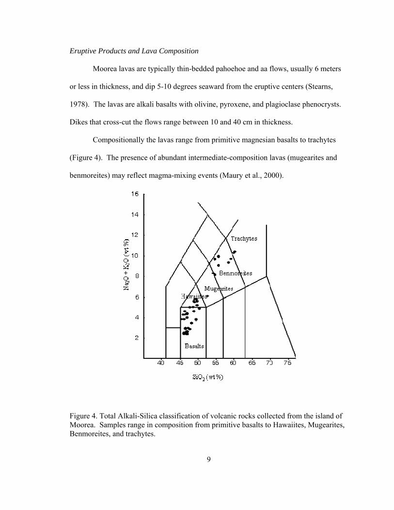
Eruptive Products and Lava Composition
Moorea lavas are typically thin-bedded pahoehoe and aa flows, usually 6 meters
or less in thickness, and dip 5-10 degrees seaward from the eruptive centers (Stearns,
1978). The lavas are alkali basalts with olivine, pyroxene, and plagioclase phenocrysts.
Dikes that cross-cut the flows range between 10 and 40 cm in thickness.
Compositionally the lavas range from primitive magnesian basalts to trachytes
(Figure 4). The presence of abundant intermediate-composition lavas (mugearites and
benmoreites) may reflect magma-mixing events (Maury et al., 2000).
Figure 4. Total Alkali-Silica classification of volcanic rocks collected from the island of Moorea. Samples range in composition from primitive basalts to Hawaiites, Mugearites, Benmoreites, and trachytes.
10
Previous Work
Mantle Plumes and Hotspot Volcanism
Mantle plumes that produce intraplate volcanism appear to be around 200ºC
hotter than ambient upper-mantle temperatures (Okal, 1987). Assumed plume viscosities
are only slightly lower than those of the surrounding mantle, meaning that a vertical,
axisymmetric plume cannot ascend freely through the mantle (Duncan et al., 1994). The
surrounding mantle will instead be viscously coupled to the plume and ascend with it as a
sheath-like boundary layer that can be hundreds of kilometers thick. Further reduction in
the viscosity contrast between plume and mantle is caused by conductive heat loss from
the plume into this boundary layer material, which also has the effect of increasing the
buoyancy of the boundary layer.
Duncan et al. (1994) suggest that the plume continuously entrains surrounding
mantle as it ascends, such that the material closest to the center of the plume will ascend
from the deepest levels, while the outer parts of the plume will be entrained at relatively
shallow levels. The “hotspot”, then, is concentrically zoned with deep, hot plume
material at its core and progressively shallower and cooler mantle material approaching
its margins. When this rising structure encounters temperature/pressure conditions for
melting in the upper mantle, the entrained materials melt to a lesser degree than the core
plume mantle because the entrained material temperature is lower. Given that the upper
mantle is chemically more depleted than the plume core (i.e. it has lower abundances of

11
incompatible elements and volatiles), it should melt to far lower extents at a given
temperature than the core of the plume.
The highest extents of melting observed in intraplate settings correlate with the
passage of the plume core beneath the hotspot volcano – thus the highly voluminous
eruptions observed at Kilauea and Mauna Loa, which sit above the core of the Hawaiian
hotspot. As volcanoes are carried away from the plume core by plate motion, smaller-
degree melts of cooler outer plume rocks are increasingly dominant, and volcanic activity
fades. This pattern has been observed in the eruptive histories of other intraplate sites
and is considered a reasonable model for the volcanic history of an island in the Society
chain.
Until now, no one has conducted a comprehensive examination of the petrology
of Moorea lavas. However, lavas from Tahiti have been studied in some detail (Duncan
et al., 1994). Mean Nd concentrations increase with time in Tahitian lavas, which means
that the mean degree of melting must therefore have decreased with time. Based on εNd
abundance and isotope systematics, Duncan et al. (1994) suggest that 5-15% melting
produced the earliest magmas, while as little as 1-2% melting produced late-shield and
late-stage magmas. These late-stage samples with the highest Nd are believed to be
derived from a source consisting predominantly of depleted mantle with less than a 10%
admixture of material from the Society plume.
As noted by Duncan et al. (1994) and others, the Society Islands are dominated by
alkali basalts, which are poorer in SiO2 and richer in alkalis than tholeiites, consistent
with lower extents of melting (Green and Ringwood, 1966). Pb/Ce ratios in Society
basalts are typical to slightly higher than the values of other oceanic basalts and appear to

12
be a feature of their mantle source. Hofmann and White (1982) used this parameter to
suggest that the incompatible-element enrichments which characterize the Society plume
are due in part to deep recycling of continental-crustal material, such as subducted
continental sediments. Elevated Sr and Pb isotopic ratios are also consistent with the
hypothesis.
Geochemistry of Hotspot Volcanics
Hotspot volcanics can preserve extreme variability in Sr, Nd, and Pb radiogenic
isotopic ratios and noble gas isotopes (i.e. radiogenic isotopic ratios of He, Ar, and Xe)
within a chain and even within different magma stages of a given island (Zindler and
Hart, 1986; Hart, 1988; Kurz and Jenkins, 1982; Staudacher and Allegre, 1981).
Explanations of radiogenic isotopic systematics in ocean islands require multiple isotopic
reservoirs in their mantle sources. As many as eight reservoirs (Zindler and Hart, 1986)
and as few as four (Hart, 1988) are described in the literature. Hofmann and White
(1982) were early proponents of the idea that subducted ocean crustal materials
incorporate into one or more of these isotopic reservoirs. Subsequent studies focused on
the possible subduction origins of three reservoirs, named (originally by Zindler and Hart,
1986) HIMU, EMI and EMII.
Hart (1988) and others contend that the “enriched” radiogenic isotope signature of
the EMII reservoir (i.e., high 87Sr/86Sr, low 143Nd/144Nd, high 206Pb/204Pb and 207Pb/204Pb)
is consistent with the likely signatures of subducted sediments. The EMII signature is
largely limited to the southern Pacific ocean (i.e., Dupre and Allègre, 1981), and studies
13
suggest that it originates from a “graveyard” of subducted slabs in the mantle beneath the
SE Pacific region (i.e. Castillo et al., 1996).
Previous Work on B, Be, Li in Ocean Islands
The relatively broad support for a subducted sediment origin for some ocean
island sources aside, workers focusing on the geochemistry of downgoing slabs warn that
metamorphic changes associated with progressive subduction profoundly impact the
incompatible-element and isotopic ratios of subducted materials. Direct comparisons of
the compositions of surficial materials and the geochemical signatures of hotspot lavas
are unlikely to lead to useful conclusions, which is particularly true for the “fluid mobile”
elements (e.g., Leeman, 1996) including B, Cs, Pb and (in some cases) Li.
Boron is one of the most powerful indicators for slab involvement used in studies
of arc petrogenesis (Ryan and Langmuir, 1993; Ryan et al., 1996). Ryan et al. (1996),
suggest that devolatilization of subducting plates segregates B into crustal reservoirs and
returns large volumes of B-depleted material to the deep mantle. Materials from the deep
mantle may preserve a distinctly depleted B signature and record the effects of ancient
subduction events. B content ranges between 3 and 6 ppm in the majority of ocean island
alkali basalts and shows greater relative variation than Be, Ce, or K, indicating that it
behaves less compatibly during melting and crystallization (Ryan et al., 1996). Primitive
mantle abundance estimates for B range between ~0.5 and <0.1 ppm (Leeman and
Sisson, 1996).
Dostal et al. (1996) studied Li, Be, and B variations in submarine lavas from
various islands in French Polynesia. Their results show that OIBs from this region have

14
higher B contents than MORBs. Looking at Li/Be and B/Be ratios, Dostal et al. (1996)
concluded that Li and B are most likely removed from down-going slabs during
subduction-related metamorphism and are not involved in deep-level mantle recycling.
Boron values greater than 5 ppm for intraplate lavas as reported by Dostal et al. (1996)
are suspect. Because seawater contains ~4.5 ppm B, the use of submarine lava samples
may skew the range of B contents to higher values.
While B contents are higher in MORBs than OIBs, uniformly lower B/K and
B/Nb ratios in the lavas indicate that all intraplate source regions, regardless of their
isotopic characteristics, experienced boron depletion (Ryan et al., 1996). Chaussidon and
Marty (1995) examined the B-isotope systematics of submarine intraplate lavas, finding
values between -14.6 and -4.3‰ (light compared to MORBs with values of -6.5 to -1.2
‰). They presumed these light values were “primitive” and suggested that assimilation
of small amounts of altered basaltic crust may account for the higher boron ratios of
MORBs and back-arc basin basalts (BABBs -8.0 ± 1.5 to +7.5 ± 1.5 ‰). Similar ranges
of values have not been encountered in studies of subaerial intraplate whole rocks
(generally δ11B in subaerial lavas are somewhat higher: S. Tornarini, unpubl.), and the
lack of reference samples determined both via TIMS and ion microprobe makes this
dataset problematic to integrate.
In contrast to Chaussidon and Marty (1995), Ryan et al. (1996) suggest that all
OIBs show B depletions related to a global event (probably continental crust formation)
that generated two mantle reservoirs with distinct B abundances. It is likely that fine
distinctions between OIB sources developed episodically as more B-depleted subducted
materials were added to the mantle (Ryan et al., 1996).
15
Lithium is a moderately incompatible trace element that is concentrated in
sediments and altered oceanic crust relative to mafic igneous rocks, is soluble in
hydrothermal fluids, and behaves similarly to Yb during fractional crystallization and V
during melting present in ocean ridge settings. Peridotite and basalt data suggest a
mantle content of 1.9 ppm Li and indicate that significant Li resides in olivine and
orthopyroxene (Ryan and Langmuir, 1987; Seitz and Woodland, 2000). The Li content
for MORBs, from the most picritic to the most evolved, ranges from 3 to 15 ppm.
Basalts usually contain less than 8 ppm Li (Ryan and Langmuir, 1987).
Lithium isotopic signatures (δ7Li) distinguish seawater from oceanic basalts and
are elevated in altered crustal rocks (Chan and Edmond, 1988; Chan et al., 1992).
Subduction may fractionate Li isotopes, such that deeply subducted slabs of isotopically
light Li generate distinct reservoirs that can be sampled by plume-related magmas (Zack
et al., 2003). While δ7Li in altered MORBs ranges from +4.5 to +14 ‰, eclogites studied
by Zack et al. (2003) have dramatically lower values, from -11 to +5 ‰. Low δ7Li in
eclogites is inferred to be produced by Rayleigh distillation-style isotope fractionation
during the early stages of metamorphism (Zack et al., 2003). Processes that may also
contribute to low δ7Li in these eclogites are seafloor alteration of their basaltic protoliths,
fluid exchanges between the eclogites and their surrounding garnet mica schist during
high-grade metamorphism, and fluid loss during prograde metamorphism (Zack et al.,
2003).
Samples of ultramafic xenoliths presumed to reflect an EMII mantle source have
δ7Li of +4 to +7 ‰ (Nishio et al., 2004). These values are comparable to those reported
for terrestrial volcanic rocks. Anhydrous ultramafic samples presumed to represent EMI-
16
type mantle (based on radiogenic isotopes) have δ7Li of <-17 ‰ (Nishio et al., 2004).
Serpentinites of the Mariana forearc studied by Benton et al. (2004) range in δ7Li from -6
to +10‰, indicating complex processes of Li isotopic exchange during slab-fluid/mantle
exchanges in shallow subduction systems.
Ocean-island basalts studied for Li isotopes include samples from Mt. Erebus and
other sites examined by Ryan and Kyle (2004) and lavas from several Hawaiian volcanic
centers (Tomascak et al., 1999; Chan and Frey, 2003). δ7Li in these lavas range from +3
to +7‰, values nearly indistinguishable from MORBs. No OIB sample studied thus far
shows the low values inferred by Nishio et al. (2004) as indicative of the EMI reservoir.
An explanation for the MORB-like Li isotopic values offered by Ryan and Kyle (2004) is
mixing between plume material and the MORB-like upper mantle results in the dilution
of whatever “plume signature” may have been present.
The bulk solid/liquid distribution coefficient for beryllium during melting of the
mantle and crystallization of basalts is 0.03-0.06 making Be a strongly incompatible trace
element, similar in its behavior to neodymium (Ryan and Langmuir, 1988). Be
abundances in alkaline intraplate basalts (1-10 ppm) are up to five times greater than
those of MORBs (0.15-2.5 ppm) and correlate with higher abundances of Zr, Nd and
other incompatible lithophile elements. Ratios of Be/Nd and Be/Zr in intraplate basalts
are very similar to those of MORBs. More evolved alkaline basalts show larger
variations in Be/incompatible element ratios with progressive differentiation (Ryan,
2002).

17
Sampling and Analysis
Sample Collection
In August 2001 and March 2003, I collected over 40 different samples on
Moorea, mostly along the coastal road that encircles the island but a few further inland
(Figure 5). Dr. William White at Cornell University provided characterized basalt
samples from other islands in the Society chain.
Figure 5. Island of Moorea with sample names and locations (small red dots). Rock types are noted if they differ from digitized geology. Black stars indicate points of interest on the island.

18
Petrology/Petrography
The following descriptions are from twenty thin sections from the freshest
samples representing all the different rock types.
Primitive and evolved basalts are aphyric to moderately porphyritic and contain
phenocrysts of olivine and pyroxene in a groundmass of olivine, pyroxene, opaques
(magnetite, illmenite) and microphenocrysts of plagioclase. Inferred order of
crystallization is olivine+plag, followed by clinopyroxene and later opaques. Olivine and
pyroxenes range from euhedral to anhedral depending on alteration; some have distinct
reaction rims, and some are zoned (Figure 6). Microscopic zeolite crystals (natrolite,
phillipsite, analcime, etc.) are present in some samples.
Figure 6. Primitive basalt (M01Fish2D) with subhedral olivine and euhedral pyroxene with reaction rim phenocrysts. Zeolites line the rim of vesicles (40X).
Olivine Olivine
pyroxene
zeolites

19
Hawaiites and mugearites contain ~1-mm plagioclase phenocrysts in a fine
groundmass (60% plagioclase, 30% opaques, 10% pyroxene for hawaiites, predominantly
plagioclase in mugearites). Some contain clinopyroxenes and zeolites. Textures range
from subophitic to intersertal or felty (Figure 7).
Figures 7. M01 B2B hawaiite in plain & crossed-polarized light, plagioclase microphenocrysts with euhedral olivine glomerocryst intergrowth (40X).
olivine
Plagioclase
20
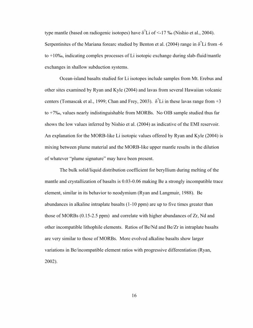
The benmoreites (intermediate lavas) are massive and variably vesicular with a
trachytic texture (Figures 8). Zeolites are present in the vesicles of a few of the
benmoreite samples, indicating hydrous alteration.
Figures 8. M01 PK 25N Benmoreite with trachytic texture (plagioclase, spinel, pyroxene microphenocrysts) 40X.
21
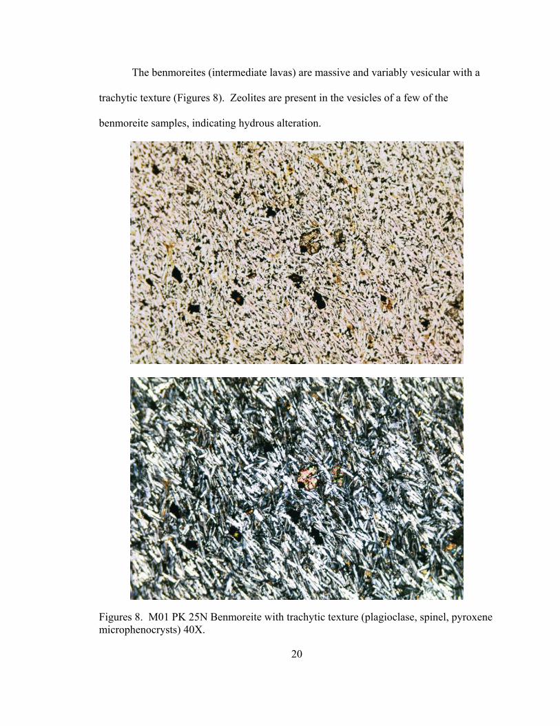
One benmoreite sample, M01PK-19N, contained a pyroxene xenolith, 2 cm x 3
cm (Figures 9). I observed a similar xenolith measuring 6 cm x 8 cm in the area where I
collected the sample.
Figures 9. Pyroxene xenolith on left, right side is groundmass with microphenocrysts of plagioclase, olivine, and pyroxene, plain & crossed-polarized (40X).
pyroxene

22
Although samples appear fresh, in thin section most samples show some degree of
alteration due to weathering (i.e. olivine oxidation and removal, or reddening of the
groundmass).
23
Geochemical Methods
I prepared and analyzed samples collected in Moorea in 2001 for major and trace
elements as part of a senior thesis project. I used similar methods for samples collected
in 2003.
Major and Trace Elements
I utilized a LiBO2 fluxed, fusion digestion procedure modified from that of
Tenthorey et al. (1996) to prepare samples for major and some trace-element
measurements. For samples collected in 2001, I diluted a 5-ml aliquot of the
lithium/beryllium solution with an equal amount of 2M HNO3 + 2000 ppm LiCO3. I
added a germanium spike to dilution acids to serve as a performance monitor for the
plasma spectrometry measurements and performed the analyses for major and trace
elements using the Direct Current Plasma-Atomic Emission Spectrometer (DCP-AES) at
the University of South Florida.
Light Elements
I selected 20 of the freshest Moorea samples for Li, Be, and B analysis along with
13 well-characterized basalt samples from other Society Islands (White et al., 1996;
Table 3). I prepared samples for Li and Be analysis following the HF-HClO4 acid
digestion method outlined in Ryan and Langmuir (1987). I used two boron digestion
protocols: an HF-HCl-mannitol acid digestion method modified from Ishikawa &

24
Nakamura (1992) for samples collected in 2001, and a Na2CO3 fluxed fusion technique
modified from that of Ryan and Langmuir (1993) for samples collected in 2003. The two
methods yielded comparable results for the very low B concentrations of the samples. I
used standard additions methods to determine all light-element abundances. Samples
were measured for B, Li and Be abundances by the (DCP-AES) at the University of
South Florida. Analytical precision for Li and Be measurements are routinely ±5%;
uncertainties for boron measurements at the low abundance levels of these samples are in
the ±10-25% range.
Lithium Isotopes
I analyzed six samples from Moorea and six samples from other islands in the
Society chain for Li isotopes. The Moorea samples reflect both the range of
differentiation represented in the suite and some variation in degree of weathering, based
on the presence/absence of zeolite phases and other indicators. The other Society Islands
samples chosen were the most primitive samples available (based on high MgO
contents), with the intent of trying to define both the "mantle" signature for Li isotopes,
and any temporal variation in the signature that may have occurred.
Sample preparation for Li isotopic analysis was at the Department of Geology at
the University of Maryland and followed an HF:HNO3:HCl digestion. Samples dripped
through a three-column separation method modified from that of Moriguti and Nakamura
(1998), in particular in that the third column is pressurized with N2 to facilitate
separation. On occasion, samples are passed through the third cation column a second
time to improve separation of Na from Li, as excess Na in samples results in spurious Li
25
isotopic measurements. Typically, only samples with qualitative Na/Li intensity ratios of
5 or less are analyzed for isotopic ratios: for my samples, the Na/Li ratios were 3 or less.
Lithium-isotopic-ratio measurements were conducted using the NU Plasma
doubly focusing multi-collector-inductively coupled plasma source mass spectrometer
(MC ICP-MS). Sample measurements are bracketed by measurements of the Li isotopic
standard L-SVEC to correct for isotopic fractionation and further calibrated to
determinations of in-house standards UMD-1 (+55‰) and IRMM-1 (-0.7‰). Lithium
isotope values are expressed as per-mille variations from the L-SVEC Li isotopic
standard (δ7Li) based on the following formula:
1000*
6
7
6
7
6
7
6
7
LSVEC
LSVECsample
LiLi
LiLi
LiLi
LiLi
⎟⎟⎠
⎞⎜⎜⎝
⎛
⎟⎟⎠
⎞⎜⎜⎝
⎛−⎟⎟
⎠
⎞⎜⎜⎝
⎛
=δ
Typically, measured Li isotopic ratios for L-SVEC lie between 13.1 and 13.5,
~10% higher than the accepted 7Li/6Li value of 12.01. As the measured values for L-
SVEC vary by less than 2‰ during the course of a run, it is possible to correct directly to
determine δ7Li values for bracketed unknowns.
The accuracy of the measurements is assessed through measurements of reference
samples JB-2 (+4.5‰) and BHVO-2 (+5‰). In all cases, the measurements are within
1‰ of accepted values in all runs.
26
Results
The elemental and isotopic data for the Moorea and Societies samples are in
Tables 1-4 and Figures 10-17.
Major Element variations
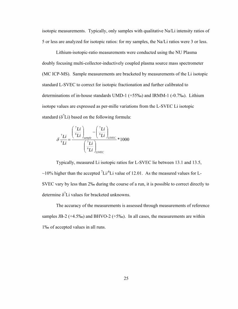
Based on the McDonald and Katsura classification scheme (1964), the samples
from Moorea plot within the Hawaiian alkalic basalt field (Figure 10). SiO2 ranges from
46 to 60 wt % . TiO2 contents increase steadily with decreasing MgO contents up to 5 wt
%; however, in the most evolved rocks (Benmoreites and Mugearites), TiO2 is less than
1.5 wt % indicating crystallization of magnetite within the magma chamber (Figure 11).
0
2
4
6
8
10
12
44 46 48 50 52 54 56 58 60
SiO2 (wt %)
Na 2
O +
K2O
(wt %
)
Tholeiitic
Alkalic
Figure 10. All Moorea samples plot within the alkalic field (Modified from McDonald & Katsura, 1964).

27
0.0
0.5
1.0
1.5
2.0
2.5
3.0
3.5
4.0
4.5
0.0 2.0 4.0 6.0 8.0 10.0 12.0 14.0 16.0 18.0
MgO (wt %)
TiO
2 (w
t %)
SocietiesMoorea
PRIMITIVE
EVOLVED
Figure 11. TiO2 contents increase with decreasing MgO. At ~5% Magnesium, titanium decreases sharply indicating the crystallization of magnetite in the magma chamber.
Trace Elements
Concentrations of trace transition metals are consistent with those of alkali
basalts. Ni and Cr abundances correlate positively with MgO. Zn abundances range
from 95 to 115 ppm. Cu abundances range from 57 to 82 ppm. The Cu/Zn ratio is < 1
(characteristic of alkali basalts; Table 1-2).
Magmas with Ni of 200-300 ppm have likely experienced little olivine
crystallization or accumulation (Hart and Davis, 1978; Sun and Hanson, 1975). Ni
analyses of the Moorea samples lie within this range and confirm their primitive
character. The Moorea samples form a continuous spectrum from primitive basalts to
trachytes. As indicated on a plot of Ni vs. TiO2, fractional crystallization appears to be
the dominant magmatic process of the formation of the suite of rocks (Figure 12).
28
0
100
200
300
400
500
600
0 5 10 15 20 25 30
TiO2 (wt %)
Ni (
ppm
) predicted ClMoorea samplesSocieties20%
50%
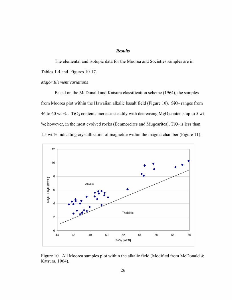
Figure 12. Samples from Moorea and other Society islands follow a predicted model for fractional crystallization for a range of F from 1.0 to 0.5. The most evolved Moorea sample erupted when approximately 50% of the magma chamber had crystallized.
B-Be-Li Concentrations
Lithium abundances vary from 2.9 to 13.2 ppm and Be contents from 1.0 to 3.0
ppm. Both elements increase with progressive differentiation.(Figure 13). Boron
contents are 1.0 ─ 3.2 ppm. Excluding samples with zeolite alteration, the range in boron
abundances is even narrower (1.0 ─ 2.4ppm).

29
0
2
4
6
8
10
12
14
0 2 4 6 8 10 12 14 16 18
MgO (wt%)
Li (p
pm)
SocietiesMoorea
0.0
0.5
1.0
1.5
2.0
2.5
3.0
3.5
0.0 2.0 4.0 6.0 8.0 10.0 12.0 14.0 16.0 18.0
MgO (wt%)
Be
(ppm
)
SocietiesMoorea
Figure 13. Li vs MgO (a) and Be vs MgO (b) contents for Moorea (turquoise squares), and Society Islands (navy squares) with similar trajectories suggestive of similar parental source. Both Li and Be increase with progressive differentiation.
a
b
30
Lithium and beryllium abundance systematics in the Society lavas are similar to
those reported for other ocean island basalts. Li and Be abundances both increase with
increasing SiO2 and decrease with increasing MgO contents, suggesting that both
elements behave incompatibly during differentiation processes that occur at ocean
islands. Samples from Moorea and the other Society Islands show broadly similar
trajectories, perhaps indicating a similar parental source.
The Li/V ratios average ~0.02 consistently, indicating that Li and V behave
similarly in OIBs, just as they do in MORBs and that the Li/V ratios of primitive MORBs
and OIBs are similar (Ryan and Langmuir, 1987: Table 3).
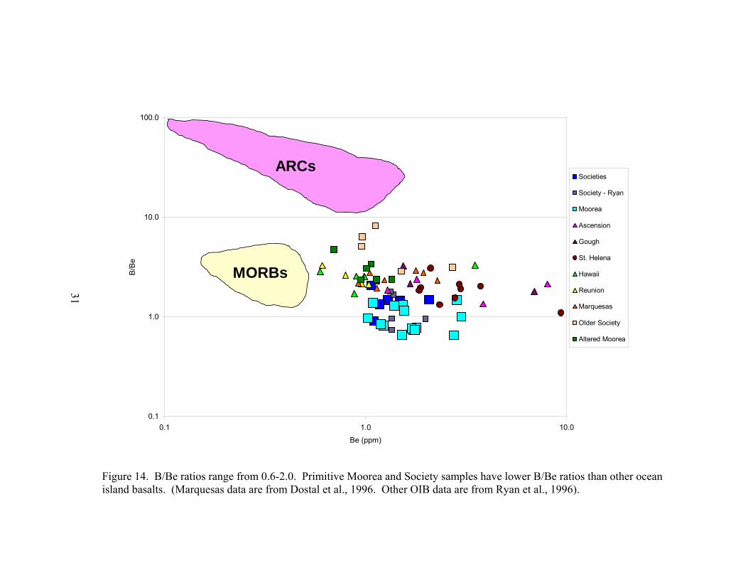
B/K2O and B/Be ratios for basaltic lavas are 0.7 ─ 1.4 and 0.6 ─ 1.3, respectively,
while more-evolved samples have somewhat higher values. Comparison to other ocean
island basalts (Dostal et al., 1996; Ryan et al., 1996) shows that the ratios are similar to
those for other Society Islands lavas and lower than those for St. Helena, Hawaii, Gough
and Ascension, as well as analyzed MORB. These low B/Be and B/K ratios are
consistent with a mantle source that includes boron-poor subducted materials (Figures 14
and 15).
31
0.1
1.0
10.0
100.0
0.1 1.0 10.0Be (ppm)
B/B
e
Societies
Society - Ryan
Moorea
Ascension
Gough
St. Helena
Hawaii
Reunion
Marquesas
Older Society
Altered Moorea
ARCs
MORBs
Figure 14. B/Be ratios range from 0.6-2.0. Primitive Moorea and Society samples have lower B/Be ratios than other ocean island basalts. (Marquesas data are from Dostal et al., 1996. Other OIB data are from Ryan et al., 1996).
31

32
0.1
1.0
10.0
100.0
0.01 0.10 1.00 10.00 100.00
K2O (wt %)
B/K
2O
SocietiesSociety - RyanMooreaAscensionGoughSt. HelenaHawaiiReunion
MORBs
ARCs
Figure 15. B/K2O ratios range from 0.7-2.0. Moorea values are similar to other Society Islands and lower than those for St. Helena, Hawaii, Reunion and Ascension. Ascension, Gough, St. Helena, Hawaii and Reunion data are from Ryan et al., 1996.
32
33
Lithium Isotopes
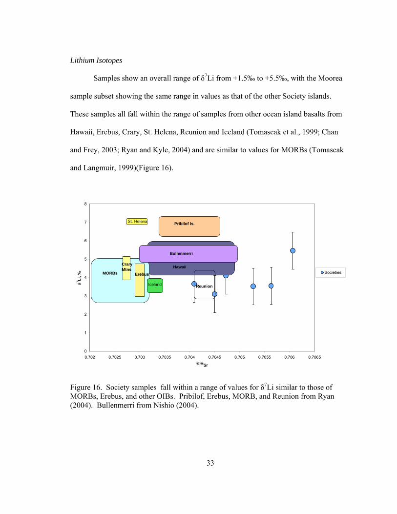
Samples show an overall range of δ7Li from +1.5‰ to +5.5‰, with the Moorea
sample subset showing the same range in values as that of the other Society islands.
These samples all fall within the range of samples from other ocean island basalts from
Hawaii, Erebus, Crary, St. Helena, Reunion and Iceland (Tomascak et al., 1999; Chan
and Frey, 2003; Ryan and Kyle, 2004) and are similar to values for MORBs (Tomascak
and Langmuir, 1999)(Figure 16).
0
1
2
3
4
5
6
7
8
0.702 0.7025 0.703 0.7035 0.704 0.7045 0.705 0.7055 0.706 0.706587/86Sr
δ7 Li, ‰
Societies
Reunion
Pribilof Is.
MORBs Erebus
CraryMtns
Bullenmerri
Hawaii
St. Helena
Iceland
Figure 16. Society samples fall within a range of values for δ7Li similar to those of MORBs, Erebus, and other OIBs. Pribilof, Erebus, MORB, and Reunion from Ryan (2004). Bullenmerri from Nishio (2004).
34
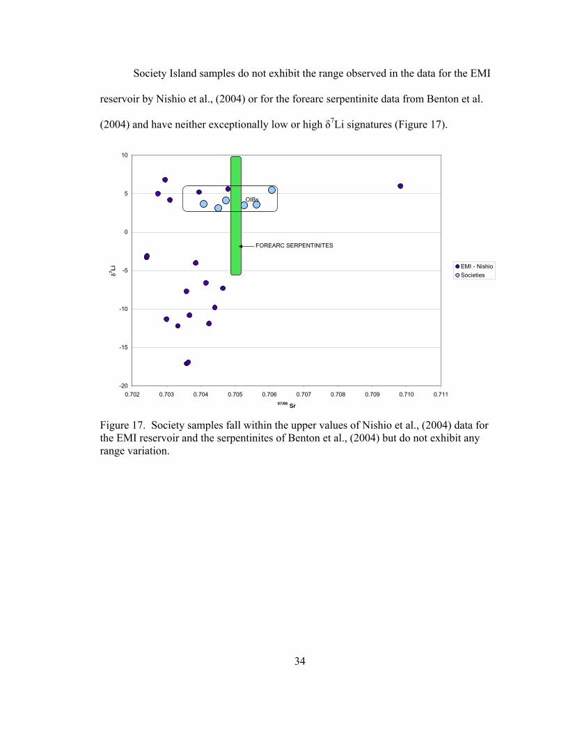
Society Island samples do not exhibit the range observed in the data for the EMI
reservoir by Nishio et al., (2004) or for the forearc serpentinite data from Benton et al.
(2004) and have neither exceptionally low or high δ7Li signatures (Figure 17).
-20
-15
-10
-5
0
5
10
0.702 0.703 0.704 0.705 0.706 0.707 0.708 0.709 0.710 0.71187/86 Sr
δ7 Li EMI - NishioSocieties
FOREARC SERPENTINITES
OIBs
Figure 17. Society samples fall within the upper values of Nishio et al., (2004) data for the EMI reservoir and the serpentinites of Benton et al., (2004) but do not exhibit any range variation.
35
Discussion and Conclusions
No simple correlations between Loss On Ignition (LOI) and Li isotopes are
evident, although it is noted that weathering processes preferentially tend to remobilize
and leach out 7Li resulting in overall lower δ7Li values (Pistiner and Henderson, 2003;
Huh et al., 2004; Rudnick et al., 2004). The Moorea samples are from a tropical island
with high relief, so it is reasonable to assume that all samples have been exposed to some
weathering. Oddly, the sample with the most noticeable alteration, M01AIR1A, has one
of the highest δ7Li values at +4.6 ‰. M01FISH2D, one of the most primitive samples,
appears to be very fresh with some surface zeolites, but it has a δ7Li value of only +1.8
‰. As zeolite formation and associated alteration is highly localized, it may be that even
visibly weathered samples contain fresh horizons, which may be preferentially sampled
during cutting, crushing and powdering; while ostensibly fresh sample segments may
nonetheless preserve evidence of concealed alteration. Clearly, the presence of any
zeolites in such samples is cause for concern in terms of obtaining a "magmatic" Li
isotopic signature. The relatively limited range of values for the Moorea samples, and
their similarity to those of fresh Society Island basalts, indicates that absent fresher
samples, older lavas may be used to define Li isotopic minima.
As with other OIBs, boron and boron ratios are very low (the lowest compared
with all other OIBs examined thus far) for Moorea and other Society Island samples

36
indicating a source region that is depleted in B. Li and Be abundances are also similar to
other OIBs pointing to similar behavior and source abundances.
Li isotope ratios in fresh lavas are similar to Hawaii, Erebus and several other
ocean islands sites, but not to St. Helena or the Pribilof Islands. The total δ7Li range of
measured intraplate lavas, at ~4‰, is similar to that observed in MORBs, and offset to
only slightly higher values. My samples from the Society Islands are very similar in their
δ7Li to MORBs.
A question inherent in these data is why Li isotopes suggest little difference
between the source regions of the Society Islands and MORBs, while B data (in
particular B/K ratios) point to significant differences between the Society Islands source
mantle and that of MORBs or other intraplate lavas, such as Hawaii (Figure 18).
Entrainment of upper mantle material into the plume (see Duncan, 1994) is a
viable means for producing largely similar δ7Li values in such volcanic systems. The
mean δ7Li is +3‰ for Society Island samples, while published data for Hawaiian lavas
are around +5‰ (Tomascak et al., 1999; Chan and Frey, 2003). Both are within error of
average MORB values (at +4‰: Tomascak and Langmuir 1999). Entrainment means
that variable amounts of a MORB source mantle is sampled during hotspot melting. The
more upper mantle material entrained, the greater the dilution of the plume signature in
the resultant melts, and the more MORB-like the lavas become.

37
Figure 18 A) Basalts erupted at the Society Island plume are alkalic in composition due to lower temperatures, higher pressure, and/or smaller degree of partial melting. B) Typically, tholeiitic basalts are erupted from the Hawaiian plume due to higher temperatures, lower pressure and/or higher degrees of partial melting. The similar δ7Li values imply that the upper mantle and deep mantle have similar Li isotopic compositions. Whereas, the differing B/K ratios imply that these plumes are sampling mantle sources with different B/K signatures.
38
Farnetani and Richards (1995), however, suggest that mantle plumes derived from
the deep mantle entrain only a very small fraction of surrounding mantle into the region
of the plume that undergoes partial melting. Vertical plume tails with a strong viscosity
contrast can entrain only a very small percentage of surrounding mantle (Stacey and
Loper, 1983; Davies, 1999).
The boron data on the Society Island samples also make the entrainment
explanation problematic. B/K ratios for the Society Islands are ~1. Hawaii B/K ratios
are ~5, and MORBs are ~10. Dilution of the plume signal by entrainment and melting of
upper mantle material should also cause B/K ratios to become similar to those of
MORBs. The differing B/K ratios of these two plumes thus imply that these plume
sources are sampling mantle sources with very different B/K signatures.
Instead of dilution by entrainment, a more viable explanation may be that the two
possible mantle sources for both the Society and Hawaii plumes and the upper mantle
have relatively similar Li isotopic compositions. Thus, it may be that recycled oceanic
crust or sediments have only a minimal influence on the Li isotope signatures of the
Society Island lavas. Data from the Society Islands suggest that δ7Li values for
subducted altered crust reported by Bouman et al. (2004) may be a more accurate
representation of the subducted δ7Li signature than original heavy values for altered crust
reported by Chan et al. (1994). The relatively low δ7Li (~+5‰) seen in high-boron lavas
from Panama (Tomascak et al., 2000) and in the serpentinite muds from the Mariana
forearc (~+6‰; Benton et al., 2004) also support a modest δ7Li signature coming from
subducted slabs.
39
PART II
Instructional Modules
Introduction
Quantitative literacy as described by the International Life Skills Survey is an
aggregate of skills, knowledge, beliefs, dispositions, habits of mind, communication
capabilities, and problem solving skills that people need in order to engage effectively in
quantitative situations arising in life and work (Briggs, 2004). Hyman Bass, American
Mathematical Society President and former chair of the Mathematical Sciences Education
Board, has noted that quantitative literacy must be taught across the curriculum, stating
“while mathematics and statistics contribute central knowledge and skills, other
disciplines provide the contexts which are so important for quantitative literacy (Steen,
2004).”During workshops for geoscience educators, however, it is repeatedly said that
students have poor mathematical skills and tend to avoid mathematics whenever possible
(Vacher, 2001). Developing material that contains mathematics to increase the
quantitative literacy of students, therefore, should be a goal for all geoscience educators.
In my experience as a student and teaching assistant, I found that one of the larger
challenges for students in undergraduate petrology classes is learning how to think
quantitatively about magmatic processes in the context of multiple geochemical
variables. This ability is necessary to understanding how major and trace elements vary
among petrogenetically related igneous rocks. It is also crucial in distinguishing igneous

40
rock suites that are derived from different mantle sources. Students face a real challenge
when they try to learn how to decipher how magmas from and evolve from elemental-
abundance data. Traditional lecture reading materials and problem sets are often found
lacking by students trying to understand the rationale underlying the interpretive
procedures.
I have prepared a series of Power Point modules for use in Petrology classes to
aid in teaching fractional crystallization and partial melting processes in the mantle.
These modules are patterned after modules of geological/mathematical problem solving
developed by H.L. Vacher and posted on the website of the Washington Center for
Improving the Quality of Undergraduate Education (The Evergreen State College) and
the Science Education Resource Center (Carleton College).
The modules I have developed are intended for use in junior/senior level
petrology or mineralogy/petrology courses where magmatic processes are normally
covered. The modules are designed to be performed by students as self-paced lab
activities or homework assignments. The goal of the modules is to help students grasp
concepts that are not easily understood through lecture or reading. The modules ask the
student users to graph geochemical data for a suite of rocks and determine whether partial
melting, fractional crystallization, or some other process dominated the formation of the
suite.
Excel spreadsheets are embedded in the modules to show students the value of
solving a problem once, then using the same spreadsheet for rapid recalculations. Use of
spreadsheets does not require any computer programming skills; therefore, only basic
computer literacy is needed. A study by Smith (1992) suggests three possible outcomes

41
for students using Excel: (1) Reversal of lack of interest in mathematics; (2)
improvement of technological literacy and enhancement of career preparation; (3)
revitalization of mathematical skills through problem solving. The content of these
modules sharpens mathematical skills by integrating algebra, logarithms, unit conversion,
and graphing.
Available geochemical modeling software, such as the Geochemist’s Workbench,
can be expensive. Such software is typically designed for researchers knowledgeable of
geochemistry, as opposed to undergraduates learning geochemistry for the first time.
Even more advanced students may be challenged in becoming proficient with these
geochemical programs. This software, along with web-based tools such as the MELTS
program, is best suited to train students to become geochemists. Excel, on the other
hand, is available on most computers, and students are often already acquainted with its
operation. The use of Excel in the modules I have developed not only helps students to
understand magmatic processes, but also helps students to develop skills that they can use
across a variety of courses and disciplines.
A study by Fratesi and Vacher (2004) of articles in the Journal of Geoscience
Education, the principal journal of earth-science teachers in the US, identified 38 articles
using spreadsheets, while less than a handful discuss the use of more sophisticated
mathematics-oriented computer programs such as MATLAB or Mathematica. Geology
provides the context needed to sharpen and develop mathematical skills. One of the
earliest articles by Ousey (1986) introduces the idea of spreadsheets for modeling
groundwater flow, an important geologic phenomenon. Spreadsheets allow students to
concentrate on the subject matter rather than the software (Beare, 1993). Students who

42
are proficient with Excel and the mathematics within the modules attain life-long skills
that transfer to other fields in geology and even other disciplines.
43
Module JAH1A and JAH1B
Fractional Crystallization
Part JAH1A of the fractional crystallization module introduces the process of
fractional crystallization through a series of explanations and calculations of partition
coefficients, bulk distribution coefficients, compatible vs. incompatible elements, and the
Rayleigh fractionation equation. The goal is to develop a way by which one can evaluate
whether progressive fractional crystallization relates the samples in a suite of volcanic
rocks and, if it does, to calculate for each sample the extent of fractional crystallization
that occurred before the lava erupted.
Module calculations use trace-element data. Trace elements simplify looking at
magmatic processes quantitatively, because their low concentrations (in the ppm range)
mean they do not play a role in the stoichiometry of crystallizing mineral phases. Trace
elements, therefore, substitute into crystals that are forming as a function of temperature,
pressure, and the overall chemical compositions of the mineral and melt. Some minor
elements, such as Ti, Mn, and K, behave as trace elements in basaltic rocks and are not
major stoichiometric constituents of the minerals that are forming (Best, 1982). It is
possible to constrain the nature of the source rock, identify what minerals (and how much
of each) melted to form a magma, and/or identify the proportions of different minerals
that may have crystallized by looking at trace-element variations in a suite of volcanic
igneous rocks.

44
The data set used in the module draws partly from the collected geochemical data
in Part I of this thesis because it is important that a suite of rocks from the same source is
used when using geochemical data to look at magmatic processes. The module begins by
defining fractional crystallization and discussing partition coefficients (Dmineral/melt) and
bulk distribution coefficients (Dsolid/melt) and incorporates a Ds/l calculation in a
spreadsheet (slides 1-7). With the introduction of the Rayleigh fractionation equation and
a spreadsheet calculation (slides 8-10), students determine if a single rock has undergone
fractional crystallization in its formation. Calculating the percentage of fractionation for
each element in a rock, however, is extremely time consuming. Looking at the
geochemistry of a suite of rocks, presumably from the same source, is a much better idea.
In slides 11 and 12, students read a discussion about the compatibility of
elements. Whether an element is compatible or incompatible depends completely on
what minerals are present in the melt. For example, when olivines and pyroxenes are
crystallizing, Sr is an incompatible element. However, as soon as plagioclase begins to
crystallize, it incorporates Sr into its crystal structure and Sr then becomes a compatible
element. The students design a spreadsheet and create a graph to help them visualize the
effects of compatibility.
The last section of part 1A of the module (slides 13-16) discusses forward
modeling. The students design a spreadsheet to calculate predicted values for a model of
fractional crystallization and then plot the given data on the model. A list of questions
posted at the end of the module can be used as a homework assignment.
Part B introduces graphical techniques as a means of identifying and calculating
fractional crystallization without making some assumptions that are necessary in part A.

45
Graphical methods rather than repetitive calculations are an excellent way to test for
fractional crystallization in a given suite of samples, and so students learn to examine
graphs to determine if fractional crystallization is the dominant process in the formation
of the suite.
In a closer look at the Rayleigh fractionation equation (slides 3-6), the module
applies logarithms and a little algebra to show students that this equation can be
configured as a line in log x vs. log y. Students then plot the data on a log-log graph.
Another spreadsheet calculates the predicted values of fractional crystallization and plots
them on the same graph showing that the samples not only fall along a straight line, but a
line that can be predicted.
The end of the module includes three data sets with instructions for students to
plot the data and determine from the plots if fractional crystallization is the dominant
process in the formation of the suite of samples. Included is a set of questions that can be
used for assessment to determine student understanding of the process of fractional
crystallization and its identification from scrutinizing graphs.
46
Module JAH2A and JAH2B
Partial Melting
Part JAH2A of the module introduces the process of magma generation due to
partial melting. Part JAH2B introduces the Shaw equation and ways to identify partial
melting. The goal is to develop a way by which one can evaluate whether partial melting
is the dominant process in a suite of volcanic rocks and, if it is, to calculate how much
melting has occurred. A statement at the beginning of the module urges students to first
work through the fractional crystallization module (JAH1) and to have a basic
understanding of phase diagrams.
Once again, the module uses trace elements because they are an excellent means
of looking at magmatic processes due to their low concentrations. Therefore, it is
possible to constrain the nature of the elements in the partial melt.
The module uses data from the geochemical analyses in part I of this thesis along
with other geochemical data from the literature. The module begins by discussing how
decreased pressure, increased temperature and change in chemical composition can each
produce partial melting (slides 3-6). A small animation (slide 7) helps students visualize
the process by which incompatible elements are enriched in the melt and compatible
elements are enriched in the mantle.
Slides 8-10 ask students to recall their knowledge of phase diagrams and calculate
the percent composition by using the lever rule. This part of the module aims for

47
students to see that melting does not move very far off the eutectic; a slight increase in
temperature produces a large increase in melt.
The second part of the module (JAH2B) introduces the Shaw equation for partial
melting. Graphs walk students through the concept of compatibility but in much less
detail than in the module on fractional crystallization. Several slides explain the type of
samples to analyze, the elemental data to use, and how to determine graphically whether
partial melting is the dominant process for a given suite of rocks. The module ends with
a few questions. Particularly instructive are questions that refer the students to new data
sets. The students must review these data sets and determine if partial melting is an
appropriate interpretation for each of them. Students must then calculate the percent of
melting for any data set that represents partial melting.
48
Evaluation of Fractional Crystallization Modules
Laura Wetzel of Eckerd College tested modules with similar design but different
geological content during the Fall 2003 semester. (Wetzel et al., 2003). During the Fall
2004 semester, I tested modules JAH1A and JAH1B at the University of South Florida to
assess improvements in student understanding of the subject of fractional crystallization.
I chose two upper-level Geology courses, Solid Earth 1 (Mineralogy/Petrology) and
Computational Geology (a course specifically designed to develop quantitative literacy).
At the beginning of the semester, each class of students answered ten questions,
four of which we used to evaluate the effectiveness of the module. The students of the
Solid Earth class (control group) received a lecture on fractional crystallization, but did
not review the module or complete any assignments. The students in Computational
Geology received the same lecture as preparation but had to work through the module
and write a paragraph evaluating its contents. I informed both classes that they would be
held responsible for the material on future exams.
One week after the lecture/assignment, I asked the same questions posed pre-
lecture to assess improvements in student understanding of the concepts and application
of fractional crystallization. Results are as follows:
49
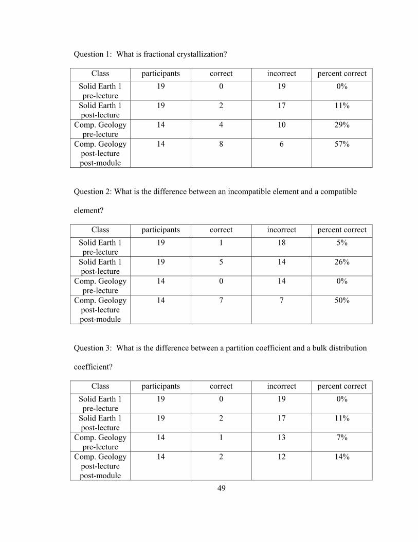
Question 1: What is fractional crystallization?
Class participants correct incorrect percent correct Solid Earth 1 pre-lecture
19 0 19 0%
Solid Earth 1 post-lecture
19 2 17 11%
Comp. Geology pre-lecture
14 4 10 29%
Comp. Geology post-lecture post-module
14 8 6 57%
Question 2: What is the difference between an incompatible element and a compatible
element?
Class participants correct incorrect percent correct Solid Earth 1 pre-lecture
19 1 18 5%
Solid Earth 1 post-lecture
19 5 14 26%
Comp. Geology pre-lecture
14 0 14 0%
Comp. Geology post-lecture post-module
14 7 7 50%
Question 3: What is the difference between a partition coefficient and a bulk distribution
coefficient?
Class participants correct incorrect percent correct Solid Earth 1 pre-lecture
19 0 19 0%
Solid Earth 1 post-lecture
19 2 17 11%
Comp. Geology pre-lecture
14 1 13 7%
Comp. Geology post-lecture post-module
14 2 12 14%

50
Question 4: When plotting a suite of samples that are dominated by fractional
crystallization, what type of trend would you expect to see on a linear graph? on a
logarithmic graph?
Class participants correct incorrect percent correct Solid Earth 1 pre-lecture
19 3 16 16%
Solid Earth 1 post-lecture
19 7 12 37%
Comp. Geology pre-lecture
14 2 12 14%
Comp. Geology post-lecture post-module
14 8 6 57%

51
Comments on Evaluation Design
Students in the control group (Solid Earth I) are mostly sophomores and juniors.
Three students in the Solid Earth class simultaneously enrolled in Computational
Geology. Their participation in the evaluation was limited strictly to their responses on
the questions posed in Solid Earth; I did not use their responses in Computational
Geology in the evaluation.
Of the 14 students in Computational Geology, only one had not yet taken Solid
Earth I. Most of the students in this class are at a senior level, and all of them have
worked through several modules on various subjects. They are not only familiar with
module design, but also with Excel spreadsheets.
Only students that attended all three classes for the pre-questions, lecture, and
post-questions were included in this study. I told both classes at the beginning of each
lecture that they would be responsible for knowing the material for upcoming exams. I
designed the lecture to cover the material presented in the modules and presented the
material in the same manner for both classes.
The students in Computational Geology worked through the module and
evaluated it, but I did not require them to turn in a homework assignment. I told the
students to contact me if they had any questions while working through the module.
Only one student asked for assistance.
A problem in the approach with the Computational Geology class arose when
several students commented that they had not had time to work through the module prior

52
to taking the exam. Consideration had to be taken that we inadvertently tested the
seriousness of the students rather than the module. I addressed this issue by asking the
students to fill out a questionnaire that included a check box stating that they had not
worked through the module prior to taking the test. Of the sixteen students that filled out
the questionnaire, 11 admitted that they had not worked through the module. Of the five
students that did work through the module, two were in the Solid Earth I class and their
results were not considered. So, only three students actually worked through the module.

53
Results
Students in Solid Earth I showed only a slight increase in understanding the
material presented in the lecture, while students in Computational Geology demonstrated
a higher increase in understanding (Figure 19). The module will be tested further,
explicitly in a Min/Pet class with the same approach as the Computational Geology class,
to see how students at this level benefit from the information.
0
10
20
30
40
50
60
Q1 Q2 Q3 Q4
Perc
ent C
orre
ct
Solid Earth PreSolid Earth postComp Geol preComp Geol post
Figure 19. Results of questions posed to students both pre- and post-lecture regarding the process of fractional crystallization.
The results of the data above suggest that working through a module can greatly
enhance student knowledge of concepts that are hard to understand through lectures or
readings. However, as I later found out, only three of the students worked through the
module. On the other hand, two of these did not answer any questions correctly pre-
lecture but answered all four questions correctly after working through the module. The
third student answered 50% of the questions correctly. Results for the three students who
carried out the experiment as it was intended are certainly encouraging.
54
Conclusions
The fractional crystallization module appears to increase understanding of the
subject matter. However, further testing of the module is required. When retested,
students should be given more time to work through the module and an assignment
should be given to make the students more accountable. Telling them that the material
would be covered on an exam did not seem to motivate them enough to work through it.
Because the modules are designed to be self-paced and worked through
individually outside the classroom, they can be an excellent supplement to lectures and
may replace textbook readings.
Another aspect noticed during the testing of the module is that modules may be a
valuable tool in exposing the deficiencies in student knowledge of basic mathematical
skills.
I did not test the partial melting module, but it is scheduled to be tested in Solid
Earth I at the University of South Florida in the Fall of 2005 along with an additional test
of the fractional crystallization module. Other modules that may be appropriate for
Petrology courses are magma mixing (in the works) and assimilation.

55
References
Beare, R., 1993. How spreadsheets can aid a variety of mathematical learning activities
from primary to tertiary level. Technology in Mathematics Teaching: A Bridge
Between Teaching and Learning. B. Jaworski. Birmingham, U.K.:117-124.
Bebout, G.E., Ryan, J.G., and Leeman, W.P., 1993. B-Be systematics in subduction
related metamorphic rocks: characterization of the subducted component.
Geochimica et Cosmochimica Acta 57:2227-2237.
Bebout, G.E., Ryan, J.G., Leeman, W.P., and Bebout, A.E., 1999. Fractionation of trace
elements by subduction zone metamorphism: significance for models of crust-
mantle mixing. Earth and Planetary Science Letters 177:69-83.
Benton, L.D., Ryan, J.G., and Savov, I.P., 2004. Lithium abundance and isotope
systematics of forearc serpentinites, Conical Seamount, Mariana Forearc: Insights
into the mechanics of slab/mantle exchange during subduction. Submitted to
Geochemistry Geophysics Geosystems
Best, M.G., 1982. Igneous and Metamorphic Petrology. New York: W.H. Freeman and
Company. 630 pp.
Binard, N., Maury, R.C., Guille, G., Talandier, J., Gillot, P.Y., and Cotten, J., 1993.
Mehetia Ialand, South Pacific: geology and petrology of the emerged part of the
Society hot spot. Journal of Volcanology and Geothermal Research 55:239-260.
Bouman,C., Elliott, T., and Vroon, P.Z., 2004. Lithium inputs to subduction zones.
Chemical Geology (In press).
56
Briggs, W., 2004. Quantitative Literacy/Reasoning. URL: http://www-
math.cudenver.edu/~wbriggs/qr/whatisit.html.
Castillo, P.R. 1996. Origin and geodynamic implication of the Dupal isotopic anomaly in
volcanic rocks from the Philippine island arcs. Geology 24,3: 271-274.
Chan, L.H., and Edmond, J.M., 1988. Variation of lithium isotope composition in the
marine environment, a preliminary report. Geochimica et Cosmochimica Acta
52,6:1711-1717.
Chan, L.H., Edmond, J.M., Thompson, G., and Gillis, K., 1992. Lithium isotopic
composition of submarine basalts; implications for the lithium cycle in the oceans.
Earth and Planetary Science Letters 108, 1-3:151-160.
Chan, L.H., Zhang, L., and Hein, J.R., 1994. Lithium isotope characteristics of marine
sediments. EOS, Transactions, American Geophysical Union 74,44 Suppl.:314.
Chan, L.H., Leeman, W.P., You, C.F., 1999. Lithium isotopic composition of Central
American Volcanic Arc lavas: implications for modification of subarc mantle by
slab-derived fluids. Chemical Geology 160:255-280.
Chan, L.H., and Kastner, M., 2000. Lithium isotopic compositions of pore fluids and
sediments in the Costa Rica subduction zone: implications for fluid processes and
sediment contribution to the volcanoes. Earth and Planetary Science Letters
183:275-290.
Chan, L.H., Leeman, W.P., and You, C.F., 2002. Lithium isotopic composition of
Central American volcanic arc lavas; implications for modificiation of subarc
mantle by slab-derived fluids; correction. Chemical Geology 182,2-4:293-300.

57
Chan, L.H., and Frey, F.A., 2003. Lithium isotope geochemistry of the Hawaiian plume:
Results from the Hawaii Scientific Drilling Project and Koolau Volcano.
Geochemistry Geophysics Geosystems 4(3):1-20.
Chaussidon, M and Jambon, A., 1994. Boron content and isotopic composition of
oceanic basalts; geochemical and cosmochemical implications. Earth and
Planetary Science Letters 121, 3-4:277-291.
Chaussidon, M. and Marty, B., 1995. Primitive boron isotope composition of the mantle.
Science 269:383-386.
Davies, G.F., 1999. Dynamic earth plates, plumes, and mantle convection. Cambridge,
UK: Cambridge Press, 458 pp.
Dostal, J., Dupuy, C., and Liotard, J., 1982. Geochemistry and origin of basaltic lavas
from Society Islands, French Polynesia (South Central Pacific Ocean).
Volcanology 45-1: 51-62.
Dostal, J., Dupoy, C., and Dudoignon, P., 1996. Distribution of boron, lithium and
beryllium in ocean island basalts from French Polynesia: Implications for the
B/Be and Li/Be ratios as tracers of subducted components. Mineralogical
Magazine 60: 563-580.
Duncan, R., Fisk, M.R., White, W.M., and Nielsen, R.L., 1994. Tahiti: Geochemical
evolution of a French Polynesian volcano. Journal of Geophysical Research 99,
B12:24,341-24,357.
Dupre, B., and Allègre, C.J., 1981. Comparative Pb-Sr-Nd isotopic studies for North
Atlantic and Indian oceans; consequences on the structure of the Earth’s mantle.
EOS, transactions, American Geophysical Union 64,17:423.
58
Dymond, Jack, 1975. K-Ar ages of Tahiti and Moorea, Society Islands, and implications
for the hot-spot model. Geology 3, 5: 236-240.
Farnetani, C.G., and Richards, M.A., 1995. Thermal entrainment and melting in mantle
plumes. Earth and Planetary Science Letters 136, 3-4:251-267.
Fratesi, S.E., and Vacher, H.L., 2004. Using spreadsheets in geoscience education:
Survey and annotated bibliography of articles in the Journal of Geoscience
Education through 2003. eJSiE 1(3):168-194.
Fiske, R.S., Rose, T.R., Swanson, D.A., and McGeehin, J.C., 1999. The Kulanaokuaiki
tephra: product of newly recognized pyroclastic eruptions at Kilauea Volcano,
Hawaii. Eos, transactions supplement, Fall meeting 1999 80,46:1196-1197.
Green, T. H. and Ringwood, A. E., 1966. Contrib. Mineral. Petrol. 18:105
Gurenko, A.A., and Chaussidon, M., 1997. Boron concentrations and isotopic
composition of the Icelandic mantle: evidence from glass inclusions in olivine.
Chemical Geology 135:21-34.
Hart, S. R. and Davis, K. E., 1978. Nickel partitioning between olivine and silicate melt.
Earth and Planetary Science Letters 40:203-219.
Hart, S.R., 1988. Heterogeneous mantle domains: signatures, genesis and mixing
chronologies. Earth and Planetary Science Letters 90:273-296.
Hauri, E.H., and Hart, S.R., 1993. Re-Os isotope systematics of HIMU and EMII oceanic
island basalts from the south Pacific Ocean. Earth and Planetary Science Letters
114: 353-371.

59
Hildenbrand, A., Gillot, P., and Le Roy, I., 2003. Volcano-tectonic and geochemical
evolution of an oceanic intra-plate volcano: Tahiti-Nui (French Polynesia). Earth
and Planetary Science Letters 6897:1-17.
Hofmann, A. W. and White, W. M., 1982. Mantle plumes from ancient oceanic crust.
Earth Planet. Science Letters 57,2:421-436.
Hofmann, A.W., 1988. Chemical differentiation of the Earth; the relationship between
mantle, continental crust, and oceanic crust. Earth and Planetary Science Letters
90,3:297-314.
Huh, Y., Chan, L.H., and Chadwick, O.A., 2004. Behavior of lithium and its isotopes
during weathering of Hawaiian basalt. Geochemistry Geophysics Geosystems 5,
9:Q09002, doi:10.1029/2004GC000729.
Ishikawa, T., and Nakamura, E., 1992. Boron isotope geochemistry of the oceanic crust
from DSDP/ODP Hole 504B. Geochimica et Cosmochimica Acta 56, 4:1633-
1639.
Kurz, M.D., Jenkins, W.J., and Hart, S.R., 1982. Helium isotopic systematics of oceanic
islands and mantle heterogeneity. Nature 297:43-47.
Leeman, W.P., Sisson, V.B., and Reid, M.R., 1992. Boron geochemistry of the lower
crust; evidence from granulite terranes and deep crustal xenoliths. Geochimica et
Cosmochimica Acta 56, 2:775-788.
Leeman, W.P., 1996. Boron and other fluid mobile elements in volcanic arc lavas;
implications for subduction processes. Geophysical Monograph 96:269-276.
Leeman, W.P., and Sisson, V.B., 1996. Geochemistry of boron and its implications for
crustal and mantle processes. Reviews in Mineralogy 33:645-707.

60
Maury, R. C., LeDez, A., Guillou, H., 2000. Moorea. Editions du BRGM Service
geologique national. 1-59.
McDonald, G.A., and Katsura, T., 1964. Chemical composition of Hawaiian lavas.
Journal of Petrology 5:82-133.
Montelli, R., Nolet, G., Dahlen, F.A., Masters, G., Engdahl, E.R., and Hung, S.H., 2004.
Finite-frequency tomography reveals a variety of plums in the mantle. Science
303:338-343.
Moriguti, T., and Nakamura, E., 1998. High-yield lithium separation and the precise
isotopic analysis for natural rock and aqueous samples. Chemical Geology
145:91-104.
Morris, J.D., and Ryan, J.G., 2003. Subduction zone processes and implications for
changing composition of the upper and lower mantle. In Carlson, JR. (Ed.)
Treastise on Geochemistry, Chapter 2: The Mantle, Chap.2.11,451-470.
Nishio, Y., Nakai, S., Yamamoto, J., Sumino, H., Matsumoto, T., Prikhod’ko, V.S., and
Arai, S., 2004. Lithium isotopic systematics of the mantle-derived ultramafic
xenoliths: implications for EM1 origin. Earth and Planetary Science Letters
217:245-261.
Okal, K., 1987. Hotspots: The First 25 Years. In Seamounts, Islands, and Atolls.
Geophysical Union. 1-11.
Ousey, JR., 1986. Modeling steady-state groundwater flow using microcomputer
spreadsheets. Journal of Geological Education 34:305-311.

61
Pistiner, J.S., and Henderson, G.M., 2003. Lithium-isotope fractionation during
continental weathering processes. Earth and Planetary Science Letters 214:327-
339.
Reisberg, L., Zindler, A., Marcantonio, F., White, W., Wyman, D., and Weaver, B., 1993.
Os isotope systematics in ocean island basalts. Earth and Planetary Science
Letters 120, 3-4:149-167.
Rose, E.F., Shimizu, N., Layne, G.D., and Grove, T., 2001. Melt production beneath Mt.
Shasta from boron data in primitive melt inclusions. Science 293, 5528:281-283.
Rudnick and Nakamura, 2004. Preface to “Lithium isotope geochemistry”. Chemical
Geology (in Press).
Ryan, J., and Langmuir, C., 1987. The systematics of lithium abundances in young
volcanic rocks. Geochimica et Cosmochimica Acta 51: 1727-1741.
Ryan, J., and Langmuir, C., 1988. Beryllium systematics in young volcanic rocks:
Implications for 10Be*. Geochimica et Cosmochimica Acta 52: 237-244.
Ryan, J., and Langmuir, C., 1993. The systematics of boron abundances in young
volcanic rocks. Geochimica et Cosmochimica Acta 57: 1489-1498.
Ryan, J.G., Morris, J., Tera, F., Leeman, B.P., and Tsvetkov, A., 1995. Cross-arc
geochemical variations in the Kurile Arc as a function of slab depth. Science
270:625-627.
Ryan, J., Leeman, W., Morris, J., and Langmuir, C., 1996. The boron systematics of
intraplate lavas: Implications for crust and mantle evolution. Geochimica et
Cosmochimica Acta 60: 415-422.

62
Ryan, J.G.,2002. The trace-element behavior of beryllium in terrestrial materials. In
Grew. E. ed.: Beryllium: Mineralogy and Geochemistry. Reviews of Mineralogy
and Geochemistry 50: 121-145.
Ryan, J.G., and Kyle, P.R., 2004. Lithium and lithium isotope variations in intraplate
mantle sources: Insights from McMurdo Group lavas (Mt. Erebus) and other
intraplate volcanic rocks. Chemical Geology 212:125-142.
Schmidt, M.W., and Poli, S., 2003. Generation of mobile components during subduction
of oceanic crust. In Rudnick, R. (ed) Treatise on Geochemistry 3: The Crust,
Chapter 3.17:567-591.
Schmincke, H.-U., 2004. Volcanism. Springer-Verlag, New York. 342pp.
Seitz, H.M., and Woodland, A.B., 2000. The distribution of lithium in peridotitic and
pyroxenitic mantle lithologies: an indicator of magmatic and metasomatic
processes. Chemical Geology 166:47-64.
Smith, R., 1992. Teaching precalculus with a spreadsheet. Fifth Annual International
Conference on Technology in Collegiate Mathematics. Rosemont, Chicago,
Illinois, Addison-Wesley.
Sleep, N.H., 1990. Hotspots and mantle plumes: Some phenomenology. Journal of
Geophysical Research 95:6,715-6,736.
Spivack, A.J., and Edmond, J.M., 1987. Boron isotope exchange between seawater and
the oceanic crust. Geochimica et Cosmochimica Acta 51:1033-1043.
Stacey, F.D., and Loper, D.E., 1983. The boundary-layer interpretation of D” and its role
as a plume source. Physics of the Earth and Planetary Interiors 33, 1:45-55.
63
Staudacher, T., and Allègre, C.J., 1982. Terrestrial xenology. Earth and Planetary
Science Letters 60:389-406.
Stearns, H., 1978. Comparison of the geology of the Society and the Hawaiian Islands.
Bernice P. Bishop Museum Occasional paper 24: 276-290.
Steen, L.A., 2004. Quantitative Literacy: Why numeracy matters for schools and
colleges. URL: http://www.maa.org/features/QL.html.
Sun, S. S. and Hanson, G. N., 1975. Origin of the Ross Island basanitoids and limitations
upon the heterogeneity of mantle sources for alkali basalts and nephelinites.
Contrib. Mineral. Petrol. 52:77-106.
Teng, F.-Z., McDonough, W.F., Rudnick, R.L., Dalpé, C., Tomascak, P.B., Chappell,
B.W., and Gao, S., 2004. Lithium isotopic composition and concentration of the
upper continental crust. Geochimica et Cosmochimica Acta (In press).
Tenthorey, E.A., Ryan, J.G., and Snow, E.A., 1996. Petrogenesis of sapphirine-bearing
metatroctolites from the Buck Creek ultramafic body, Southern Appalachians.
Journal of Metamorphic Geology 14, 2:103-114.
Thirwall, M.F., 1997. Pb isotopic and elemental evidence for OIB derivation from young
HIMU mantle. Chemical Geology 139:51-74.
Tomascak, P.B., and Langmuir, C.H., 1999. Lithium isotope variability in MORB. EOS,
Transactions American Geophysical Union Supplement 80, F1086-1087.
Tomascak, P.B., Tera, F., Helz, R.T., and Walker, R.J., 1999. The absence of lithium
isotope fractionation during basalt differentiation: New measurements by
multicollector sector ICP-MS. Geochimica et Cosmochimica Acta 63: 907-910.
64
Tomascak, P.B., Carlson, R.W., and Shirey, S.B., 1999. Accurate and precise
determination of Li isotopic compositions by multi-collector sector ICP-MS.
Chemical Geology 158:145-154.
Tomascak, P.B., Ryan, J.G., and Defant, M.J., 2000. Lithium isotope evidence for light
element decoupling in the Panama sub-arc mantle. Geology 28:507-510.
Tomascak, P., Widom, E., Benton, L., Goldstein, S., and Ryan, J., 2002. Control of
lithium budgets in island arcs. Earth and Planetary Science Letters 6108: 1-12.
Vacher, 2001. Better math, better geology. Geotimes 46, 3:13.
White, W.M., and Hofmann, A.W., 1982. Sr and Nd isotope geochemistry of oceanic
basalts and mantle evolution. Nature 296, 5860:821-825.
White, W.M., and Duncan, R.A., 1996. Geochemistry and geochronology of the Society
Islands: New Evidence for Deep Mantle Recycling. Earth Processes: Reading the
Isotope Code. Geophysical Monograph 95:183-206.
Williams, H., 1933. Geology of Tahiti, Moorea, and Maiao. Bernice P. Bishop Museum
Bulletin 105: 1-88.
Winter, J.D., 2001. An introduction to igneous and metamorphic petrology. Prentice
Hall, New Jersey. 697p.
Zack, T., Tomascak, P.B., Rudnick, R.L., Dalpe, C., and McDonough, W.F., 2003.
Extremely light Li in orogenic eclogites: The role of isotope fractionation during
dehydration in subducted oceanic crust. Earth and Planetary Science Letters
208:279-290.
Zindler, G. A. and Hart, S. R., 1986. Chemical Geodynamics. Ann. Rev. Earth Planet.
Science 14: 493-571.
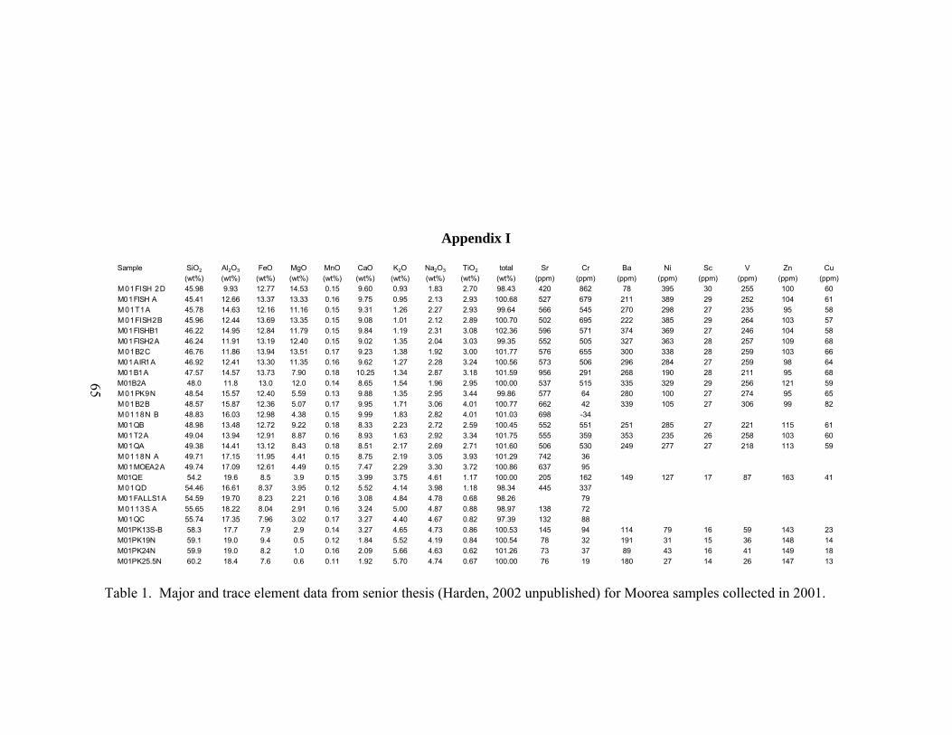
65
Appendix I
Sample SiO2 Al2O3 FeO MgO MnO CaO K2O Na2O3 TiO2 total Sr Cr Ba Ni Sc V Zn Cu(wt%) (wt%) (wt%) (wt%) (wt%) (wt%) (wt%) (wt%) (wt%) (wt%) (ppm) (ppm) (ppm) (ppm) (ppm) (ppm) (ppm) (ppm)
M01FISH 2D 45.98 9.93 12.77 14.53 0.15 9.60 0.93 1.83 2.70 98.43 420 862 78 395 30 255 100 60M01FISH A 45.41 12.66 13.37 13.33 0.16 9.75 0.95 2.13 2.93 100.68 527 679 211 389 29 252 104 61M01T1A 45.78 14.63 12.16 11.16 0.15 9.31 1.26 2.27 2.93 99.64 566 545 270 298 27 235 95 58M01FISH2B 45.96 12.44 13.69 13.35 0.15 9.08 1.01 2.12 2.89 100.70 502 695 222 385 29 264 103 57M01FISHB1 46.22 14.95 12.84 11.79 0.15 9.84 1.19 2.31 3.08 102.36 596 571 374 369 27 246 104 58M01FISH2A 46.24 11.91 13.19 12.40 0.15 9.02 1.35 2.04 3.03 99.35 552 505 327 363 28 257 109 68M01B2C 46.76 11.86 13.94 13.51 0.17 9.23 1.38 1.92 3.00 101.77 576 655 300 338 28 259 103 66M01AIR1A 46.92 12.41 13.30 11.35 0.16 9.62 1.27 2.28 3.24 100.56 573 506 296 284 27 259 98 64M01B1A 47.57 14.57 13.73 7.90 0.18 10.25 1.34 2.87 3.18 101.59 956 291 268 190 28 211 95 68M01B2A 48.0 11.8 13.0 12.0 0.14 8.65 1.54 1.96 2.95 100.00 537 515 335 329 29 256 121 59M01PK9N 48.54 15.57 12.40 5.59 0.13 9.88 1.35 2.95 3.44 99.86 577 64 280 100 27 274 95 65M01B2B 48.57 15.87 12.36 5.07 0.17 9.95 1.71 3.06 4.01 100.77 662 42 339 105 27 306 99 82M0118N B 48.83 16.03 12.98 4.38 0.15 9.99 1.83 2.82 4.01 101.03 698 -34M01QB 48.98 13.48 12.72 9.22 0.18 8.33 2.23 2.72 2.59 100.45 552 551 251 285 27 221 115 61M01T2A 49.04 13.94 12.91 8.87 0.16 8.93 1.63 2.92 3.34 101.75 555 359 353 235 26 258 103 60M01QA 49.38 14.41 13.12 8.43 0.18 8.51 2.17 2.69 2.71 101.60 506 530 249 277 27 218 113 59M0118N A 49.71 17.15 11.95 4.41 0.15 8.75 2.19 3.05 3.93 101.29 742 36M01MOEA2A 49.74 17.09 12.61 4.49 0.15 7.47 2.29 3.30 3.72 100.86 637 95M01QE 54.2 19.6 8.5 3.9 0.15 3.99 3.75 4.61 1.17 100.00 205 162 149 127 17 87 163 41M01QD 54.46 16.61 8.37 3.95 0.12 5.52 4.14 3.98 1.18 98.34 445 337M01FALLS1A 54.59 19.70 8.23 2.21 0.16 3.08 4.84 4.78 0.68 98.26 79M0113S A 55.65 18.22 8.04 2.91 0.16 3.24 5.00 4.87 0.88 98.97 138 72M01QC 55.74 17.35 7.96 3.02 0.17 3.27 4.40 4.67 0.82 97.39 132 88M01PK13S-B 58.3 17.7 7.9 2.9 0.14 3.27 4.65 4.73 0.86 100.53 145 94 114 79 16 59 143 23M01PK19N 59.1 19.0 9.4 0.5 0.12 1.84 5.52 4.19 0.84 100.54 78 32 191 31 15 36 148 14M01PK24N 59.9 19.0 8.2 1.0 0.16 2.09 5.66 4.63 0.62 101.26 73 37 89 43 16 41 149 18M01PK25.5N 60.2 18.4 7.6 0.6 0.11 1.92 5.70 4.74 0.67 100.00 76 19 180 27 14 26 147 13
Table 1. Major and trace element data from senior thesis (Harden, 2002 unpublished) for Moorea samples collected in 2001.
65
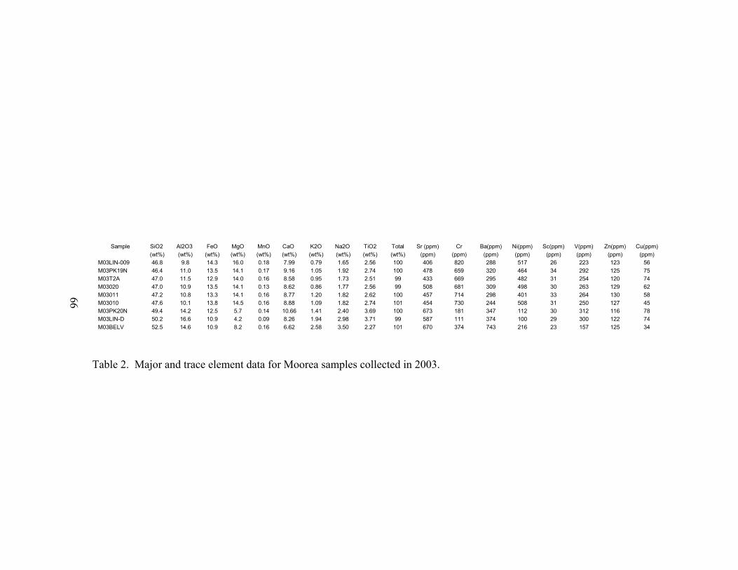
66
Sample SiO2 Al2O3 FeO MgO MnO CaO K2O Na2O TiO2 Total Sr (ppm) Cr Ba(ppm) Ni(ppm) Sc(ppm) V(ppm) Zn(ppm) Cu(ppm)(wt%) (wt%) (wt%) (wt%) (wt%) (wt%) (wt%) (wt%) (wt%) (wt%) (ppm) (ppm) (ppm) (ppm) (ppm) (ppm) (ppm) (ppm)
M03LIN-009 46.8 9.8 14.3 16.0 0.18 7.99 0.79 1.65 2.56 100 406 820 288 517 26 223 123 56M03PK19N 46.4 11.0 13.5 14.1 0.17 9.16 1.05 1.92 2.74 100 478 659 320 464 34 292 125 75M03T2A 47.0 11.5 12.9 14.0 0.16 8.58 0.95 1.73 2.51 99 433 669 295 482 31 254 120 74M03020 47.0 10.9 13.5 14.1 0.13 8.62 0.86 1.77 2.56 99 508 681 309 498 30 263 129 62M03011 47.2 10.8 13.3 14.1 0.16 8.77 1.20 1.82 2.62 100 457 714 298 401 33 264 130 58M03010 47.6 10.1 13.8 14.5 0.16 8.88 1.09 1.82 2.74 101 454 730 244 508 31 250 127 45M03PK20N 49.4 14.2 12.5 5.7 0.14 10.66 1.41 2.40 3.69 100 673 181 347 112 30 312 116 78M03LIN-D 50.2 16.6 10.9 4.2 0.09 8.26 1.94 2.98 3.71 99 587 111 374 100 29 300 122 74M03BELV 52.5 14.6 10.9 8.2 0.16 6.62 2.58 3.50 2.27 101 670 374 743 216 23 157 125 34
Table 2. Major and trace element data for Moorea samples collected in 2003.
66

67
ISLAND SAMPLE Li Be B (ppm) (ppm) (ppm)
Moorea M 01FISH 2D 4.9 1.23 1Moorea M01FISH A 5.1 1.19 1Moorea M 01T1A 5.4 1.03 1Moorea M 01FISH2B 4.7 1.52 1Moorea M01FISHB1 5.8 1.53 2Moorea M01FISH2A 6.86 1.8 1.4Moorea M 01B2C 5.9 1.39 1.8Moorea M01AIR1A 3.2 1.35 3.2Moorea M01B1A 6.6 0.95 2.24Moorea M 01PK9N 5.7 1.56 1.8Moorea M 01B2B 6.2 1.7 1.3Moorea M01QB 11.3 2.75 1.8Moorea M01T2A 7.8 1.76 1.3Moorea M01QA 13.15 3 3Moorea M03PK19N 5.8 0.7 3.3Moorea M03020 6.9 1.1 3.6Moorea M03011 12.3 2.9 4.2Moorea M03010 6.7 1.1 1.5Moorea M03LIN-D 6.5 1.0 3.1Moorea M03BELV 4.6 1.1 2.7
BoraBora 101287 4.5 1.0 6.1BoraBora 101288 6.2 1.1 9.2Huahine 101211 6.3 1.0 4.9Huahine 101198 9.3 2.7 8.5Maiao MAO-113 6.6 1.5 2.2Maiao MAO 65 3.6 1.5 4.3Maupiti 73-204 5.9 1.3 1.9Mehetia MHT-101 3.7 1.1 2.2Mehetia MHT-155 4.3 1.2 1.6Tahaa Ta3F 5.4 0.9 3.0Tahaa Ta8b 5.1 1.0 3.1Tahiti 74-422 5.8 1.1 2.5Tahiti 74-437 7.0 2.1 3.1
Table 3. Li, Be, and B analysis for 20 samples from Moorea and 13 samples from other Society Islands as indicated.
ISLAND SAMPLE δ7LiMoorea M01FISH2D 1.76Moorea M01FISH A 2.29Moorea M03PK19N 4.95Moorea M01AIR 1A 4.59Moorea M03LIN-D 1.47Moorea M03BELV 4.75Huahine 101211 3.67Maiao MAO-113 4.1Maupiti 73-204 3.1Mehetia MHT-101 3.52Tahaa Ta8b 3.55Tahiti 74-422 5.47
Table 4. δ7Li values for 6 samples from Moorea and 6 samples from other Society Islands. The samples from Moorea were chosen based on increasing SiO2 to see temporal variations of δ7Li within the formation of an island and to note the affects of weathering. Samples from the other Society Islands were chosen based on low SiO2 to see temporal variation within the formation of an island chain.

68
Appendix II
Fractional Crystallization Module JAH1A
1
When magma cools and crystallizes in the Earth’s interior, the growing crystals incorporate selected chemical elements of the magma into their structure. As a result, the magma is depleted in those elements. On the other hand, elements that are not incorporated in the growing crystals are enriched in the magma. Separation of crystals from the liquid by settling, floating, or adhering to the magma chamber walls produces a magma with a different chemical composition. This process is called fractional crystallization.
Quantitative Concepts and SkillsManipulating equationsWeighted averageForward modeling
Fractional crystallization causes basaltic magmas to evolve into basaltic-andesitic magmas. Further crystallization pushes the magma toward an even more silicic composition.
Mantle Processes1A – Fractional Crystallization
Module JAH-1A
Judy Harden, University of South Florida

69
2
Part A introduces the process of fractional crystallization through a series of explanations and calculations of partition coefficients, bulk partition coefficients, compatible vs. incompatible elements, and the Rayleigh fractionation equation. The goal is to develop a way by which we can evaluate whether fractional crystallization has occurred in a suite of volcanic rocks and, if it has, to calculate how much fractional crystallization has occurred.
This module consists of two parts, A and B.
Part B introduces graphical techniques as a means of identifying and calculating fractional crystallization without making some assumptions that are necessary in part A.
About this module
3
Slides 4-7 explain the difference betweenpartition coefficients and bulk partitioncoefficients.
Slides 8-10 introduces the Rayleighfractionation equation.
Slides 11-12 explain compatibility.
Slides 13-16 uses forward modeling tolook for fractional crystallization.
Data in this module are from samples collected from the island of Moorea. Mooreais part of the Society Island Chain, French Polynesia. Two of the better-known islands of the chain are Tahiti and Bora Bora.
Moorea
Tahiti
PREVIEW
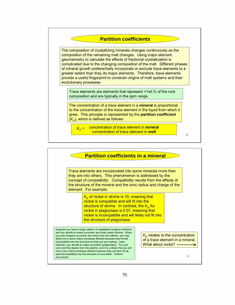
70
4
Partition coefficients
The composition of crystallizing minerals changes continuously as the composition of the remaining melt changes. Using major element geochemistry to calculate the effects of fractional crystallization is complicated due to the changing composition of the melt. Different phases of mineral growth preferentially incorporate or exclude trace elements to a greater extent than they do major elements. Therefore, trace elements provide a useful fingerprint to constrain origins of melt systems and their evolutionary processes.
concentration of trace element in mineralconcentration of trace element in melt
KD =
The concentration of a trace element in a mineral is proportional to the concentration of the trace element in the liquid from which it grew. This principle is represented by the partition coefficient(KD), which is defined as follows:
Trace elements are elements that represent <1wt.% of the rock composition and are typically in the ppm range.
5
Partition coefficients in a mineral
Suppose you have a huge caldron of vegetables (magma chamber) and you decide to make cucumber and onion salad (olivine). Whenyou pull chopped cucumber and onion from the caldron, you may likely mix in some cherry tomatoes (Nickel) because they fit well (compatible) into the structure of what you are making. Later, however, you decide to make succotash (plagioclase). You pull corn and lima beans from the caldron, and it is unlikely that you will mix in any cherry tomatoes (Nickel) because they just don’t fit as well (incompatible) into the structure of succotash. Sufferin’ Succotash!
KD of nickel in olivine is 10, meaning that nickel is compatible and will fit into the structure of olivine. In contrast, the KD for nickel in plagioclase is 0.07, meaning that nickel is incompatible and will likely not fit into the structure of plagioclase.
Trace elements are incorporated into some minerals more than they are into others. This phenomenon is addressed by the concept of compatibility. Compatibility results from the effects of the structure of the mineral and the ionic radius and charge of the element. For example:
KD relates to the concentration of a trace element in a mineral. What about rocks?

71
6
Bulk Partition Coefficient - D
To calculate D, you need to know the mass fraction (X) of the element in each mineral and the KD value for the element in each of the minerals.
D = XaKD,a +XbKD,b + XcKD,c
where a,b,and c are different minerals in the assemblage. D is the sum of the weighted average of each element in the mineral assemblage.
The bulk partition coefficient addresses the amount of trace element in a rock.
KD values are derived empirically. A good website to find these values is the Geochemical Earth Reference Model (GERM) :
http://earthref.org/GERM/index.html?main.htm
concentration of trace element in mineral assemblageconcentration of trace element in melt
D =
7
Calculate the bulk partition coefficient for nickel (DNi) in a rock that contains 10% olivine, 42% clinopyroxene, 45% plagioclase, and 3% magnetite. KD values are 10, 3, 0.07, and 48 respectively.
Once you have set up the spreadsheet to calculate DNi for the mineral assemblage, use the GERM website to find the values for titanium(KD,Ti) in the same mineral assemblage and calculate DTi. Will Ti stay in the melt or be incorporated into the crystal? Save this spreadsheet, because you will use a similar calculation later in the module.
According to your answer, will Ni stay in the melt or be incorporated into the crystal composition of the rock?
= cell containing a number.
= cell containing an equation.
Calculating D
Use the sumproductfunction in this cell.
B C D2 X K D
3 Olivine 0.1 104 Pyroxene 0.42 35 Plagioclase 0.45 0.076 Magnetite 0.03 4878 D =
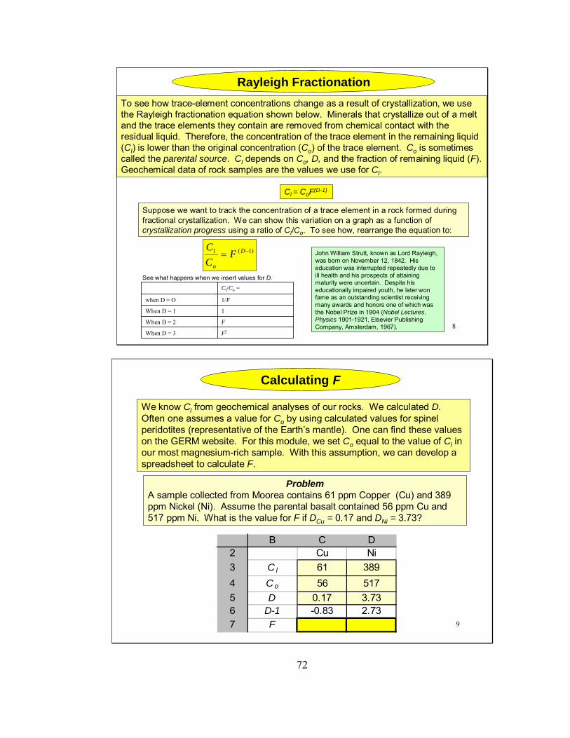
72
8
Rayleigh FractionationTo see how trace-element concentrations change as a result of crystallization, we use the Rayleigh fractionation equation shown below. Minerals that crystallize out of a melt and the trace elements they contain are removed from chemical contact with the residual liquid. Therefore, the concentration of the trace element in the remaining liquid (Cl) is lower than the original concentration (Co) of the trace element. Co is sometimes called the parental source. Cl depends on Co, D, and the fraction of remaining liquid (F). Geochemical data of rock samples are the values we use for Cl.
Cl = CoF(D-1)
Suppose we want to track the concentration of a trace element in a rock formed during fractional crystallization. We can show this variation on a graph as a function of crystallization progress using a ratio of Cl/Co. To see how, rearrange the equation to:
John William Strutt, known as Lord Rayleigh, was born on November 12, 1842. His education was interrupted repeatedly due to ill health and his prospects of attaining maturity were uncertain. Despite his educationally impaired youth, he later won fame as an outstanding scientist receiving many awards and honors one of which was the Nobel Prize in 1904 (Nobel Lectures. Physics 1901-1921, Elsevier Publishing Company, Amsterdam, 1967).
)1( −= D
o
l FCC
F2When D = 3
FWhen D = 2
1When D = 1
1/Fwhen D = O
Cl/Co =See what happens when we insert values for D.
9
Calculating F
ProblemA sample collected from Moorea contains 61 ppm Copper (Cu) and 389 ppm Nickel (Ni). Assume the parental basalt contained 56 ppm Cu and 517 ppm Ni. What is the value for F if DCu = 0.17 and DNi = 3.73?
B C D2 Cu Ni3 Cl 61 3894 Co 56 5175 D 0.17 3.736 D-1 -0.83 2.737 F
We know Cl from geochemical analyses of our rocks. We calculated D. Often one assumes a value for Co by using calculated values for spinelperidotites (representative of the Earth’s mantle). One can find these values on the GERM website. For this module, we set Co equal to the value of Cl in our most magnesium-rich sample. With this assumption, we can develop a spreadsheet to calculate F.

73
10
Calculating a value of F for each element in each sample that you have collected would be very time consuming. There is a better way of finding the percent of fractionation for your samples.
Calculating F
The answer reflects the portion of the original melt present in the magma chamber when the fractionated magma erupted to form this sample.
B C D2 Cu Ni3 Cl 61 3894 Co 56 5175 D 0.17 3.736 D-1 -0.83 2.737 F 0.90 0.90
Identical values testify that (a) fractional crystallization has occurred and (b) your geochemical analysis is accurate.
When F = 1, no crystallization has occurred (100% of the melt remains). In contrast, F = 0.1 means that 90% of the original melt has crystallized.
You should not expect every element to be exactly 0.90. Why?
11
Before we try to find F for a suite of rocks, we must fully understand compatibility. Create a spreadsheet now to see how Cl/Co changes with different values of D and F. Then plot your results as a function of F for each D value. Make the y-axis a logarithmic scale.
Compatibility
The values you calculate are the predicted values for fractionalcrystallization for any given D.
= cell containing intermediate formula
B C D E F2 D 0 1 2 33 D-1 -1 0 1 245 F Cl/Co Cl/Co Cl/Co Cl/Co
6 0.17 0.28 0.39 0.410 0.511 0.612 0.713 0.814 0.915 1

74
12
Compatibility
What you should discover with your graph is that compatible elements (D > 1) show depletion in the melt (Cl/Co < 1). Depletion occurs more rapidly the higher the value for D. Incompatible elements (D < 1) show enrichment in the melt (Cl/Co >1).
Compatible elements preferentially enter the solid phase while incompatible elements preferentially remain in the liquid phase.
0.01
0.10
1.00
10.00
0 0.2 0.4 0.6 0.8 1
F
Cl/C
o
D = 0
D = 1
D = 2
D = 3
13
Now we are ready to analyze a suite of samples to test whether fractional crystallization is the dominant process of their formation. The process we use here illustrates forward modeling where values are predicted and then tested to see if real data fit the model.
Using previously designed spreadsheets to calculate ratios
To see the maximum compositional variation, we use a compatible element and an incompatible element.
Use the spreadsheet you created in Slide 11 to predict the Cl/Co values for Ti and Ni with D values of 0.32 and 3.73 respectively. (Just type the new values for D in your chart and let Excel do the work!)
B C D2 Ti Ni3 D 0.32 3.734 D-1 -0.68 2.7356 F Til/Tio Nil/Nio7 0.18 0.29 0.310 0.411 0.512 0.613 0.714 0.815 0.916 1
After you obtain the values for Til/Tio and Nil/Nio, plot them on a graph with the Ni ratio on the y-axis and the Ti ratio on the x-axis.
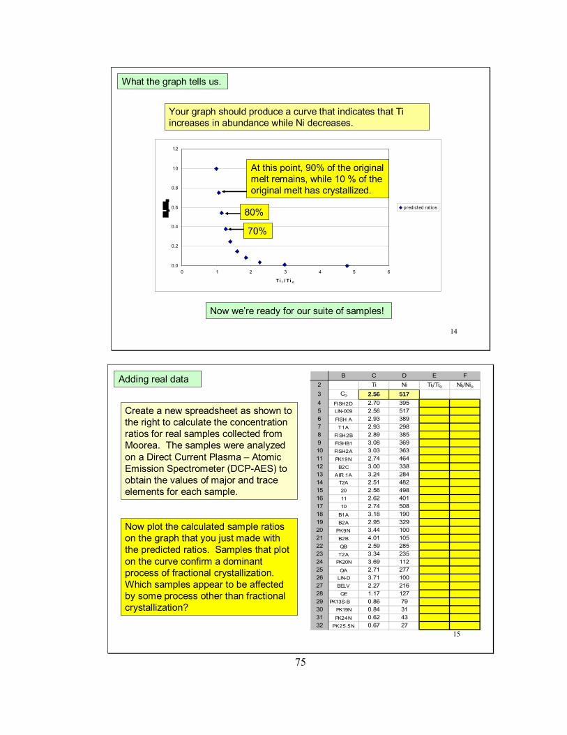
75
14
What the graph tells us.
Your graph should produce a curve that indicates that Ti increases in abundance while Ni decreases.
0.0
0.2
0.4
0.6
0.8
1.0
1.2
0 1 2 3 4 5 6
T i l / T i o
predicted rat ios
At this point, 90% of the original melt remains, while 10 % of the original melt has crystallized.
80%
70%
Now we’re ready for our suite of samples!
15
Create a new spreadsheet as shown to the right to calculate the concentration ratios for real samples collected from Moorea. The samples were analyzed on a Direct Current Plasma – Atomic Emission Spectrometer (DCP-AES) to obtain the values of major and trace elements for each sample.
Adding real data
Now plot the calculated sample ratios on the graph that you just made with the predicted ratios. Samples that plot on the curve confirm a dominant process of fractional crystallization. Which samples appear to be affected by some process other than fractional crystallization?
B C D E F2 Ti Ni Til/Tio Nil/Nio
3 Co 2.56 5174 FISH2D 2.70 3955 LIN-009 2.56 5176 FISH A 2.93 3897 T1A 2.93 2988 FISH2B 2.89 3859 FISHB1 3.08 36910 FISH2A 3.03 36311 PK19N 2.74 46412 B2C 3.00 33813 AIR 1A 3.24 28414 T2A 2.51 48215 20 2.56 49816 11 2.62 40117 10 2.74 50818 B1A 3.18 19019 B2A 2.95 32920 PK9N 3.44 10021 B2B 4.01 10522 QB 2.59 28523 T2A 3.34 23524 PK20N 3.69 11225 QA 2.71 27726 LIN-D 3.71 10027 BELV 2.27 21628 QE 1.17 12729 PK13S-B 0.86 7930 PK19N 0.84 3131 PK24N 0.62 4332 PK25.5N 0.67 27
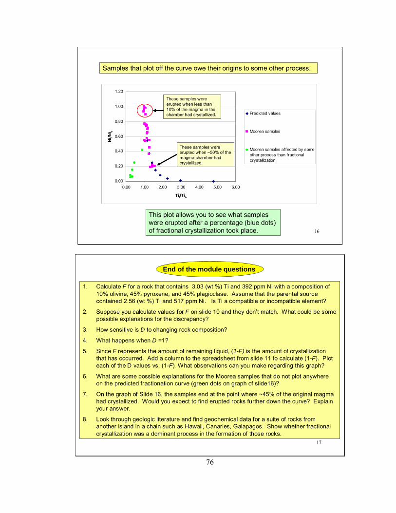
76
16
Samples that plot off the curve owe their origins to some other process.
This plot allows you to see what samples were erupted after a percentage (blue dots) of fractional crystallization took place.
0.00
0.20
0.40
0.60
0.80
1.00
1.20
0.00 1.00 2.00 3.00 4.00 5.00 6.00
Til/Tio
Ni l/N
i oPredicted values
Moorea samples
Moorea samples affected by someother process than fractionalcrystallization
These samples were erupted when ~50% of the magma chamber had crystallized.
These samples were erupted when less than 10% of the magma in the chamber had crystallized.
17
1. Calculate F for a rock that contains 3.03 (wt %) Ti and 392 ppm Ni with a composition of 10% olivine, 45% pyroxene, and 45% plagioclase. Assume that the parental source contained 2.56 (wt %) Ti and 517 ppm Ni. Is Ti a compatible or incompatible element?
2. Suppose you calculate values for F on slide 10 and they don’t match. What could be some possible explanations for the discrepancy?
3. How sensitive is D to changing rock composition?
4. What happens when D =1?
5. Since F represents the amount of remaining liquid, (1-F) is the amount of crystallization that has occurred. Add a column to the spreadsheet from slide 11 to calculate (1-F). Plot each of the D values vs. (1-F). What observations can you make regarding this graph?
6. What are some possible explanations for the Moorea samples that do not plot anywhere on the predicted fractionation curve (green dots on graph of slide16)?
7. On the graph of Slide 16, the samples end at the point where ~45% of the original magma had crystallized. Would you expect to find erupted rocks further down the curve? Explain your answer.
8. Look through geologic literature and find geochemical data for a suite of rocks from another island in a chain such as Hawaii, Canaries, Galapagos. Show whether fractional crystallization was a dominant process in the formation of those rocks.
End of the module questions

77
Fractional Crystallization Module JAH1B
1
In module 1A we demonstrated various ways of determining whether fractional crystallization was a dominant process in the formation of a suite of rocks. This module introduces the use of logarithms as a shortcut method of testing for fractional crystallization.
Quantitative Concepts and SkillsManipulating equationsLogarithmic graphing
This module should be worked only after working through module 1A.
Mantle Processes1B – Fractional Crystallization
Module JAH-1B
2
PREVIEW
Slides 3-6 Manipulate the Rayleigh fractionation equation to produce the equation of a straight line on a log-log graph
Slide 7 provides data for use on a log-log graph.
Slides 8-10 show a means of double checking your assumptions about fractional crystallization.
Slides 11-16 contain end-of-module questions in the form of data sets.
Slide 17 Pre- and Post-module questions
Note: To save time and to minimize errors, the data sets in this module are in Excel format. This means that when you are in Power Point in normal view (not in the slide show), you can double click on the data and Excel will open. You can then copy the data to a new Excel spreadsheet rather than re-type the entire data set. At that point, you can manipulate thedata by sorting or any other process.

78
3
Graphical methods rather than repetitive calculations are an excellent way to test for fractional crystallization in a given suite of samples. Using the graph made in slide 16 of module 1A requires that we know Co and D for the trace elements in order to see if our samples follow a predicted curve for fractional crystallization. By using the technique in this part of the module, we no longer need to know Co and D.
Using logarithms for graphing purposes
Logarithms and a little algebra make it possible to test whether fractional crystallization is a dominant process in the formation of a suite of rocks. It’s as easy as plotting the data on a log-log graph. Always use a compatible and incompatible element with the largest range in concentration.
To see how the method is going to work, we start with the Rayleigh fractionation equation.
Cl = CoF(D-1) (1)
4
Using logarithms for graphing purposes
Set equations 4a and 4b equal to each other and solve for log Nil. Before proceeding, write down your equation.
Take the logarithm of equation 1.
(2)FDCC ol log)1(loglog −+=
Substitute the element of interest into equation 2, and do the same for the second element of interest.
(3a)
(3b)FDNiNiFDTiTi
Niol
Tiol
log)1(logloglog)1(loglog
−+=−+=
Now, solve equations 3a and 3b for log F.
)1(logloglog−
−=
Ti
ol
DTiTiF )1(
logloglog−
−=
Ni
ol
DNiNiF(4a) (4b)

79
5
Does your equation look like the equation below? If it doesn’t,review the rules of logarithms and try again.
Using logarithms for graphing purposes
The website listed below offers easy to understand explanations of logarithm rules.
oTi
Niol
Ti
Nil Ti
DDNiTi
DDNi log
11loglog
11log ⎟⎟
⎠
⎞⎜⎜⎝
⎛−−
−+⎟⎟⎠
⎞⎜⎜⎝
⎛−−
=
http://www.purplemath.com/modules/logrules.htm
(5)
6
Using logarithms for graphing purposes
Although this equation 5 may look complicated, it is merely the equation of a straight line.
oTi
Niol
Ti
Nil Ti
DDNiTi
DDNi log
11loglog
11log ⎟⎟
⎠
⎞⎜⎜⎝
⎛−−
−+⎟⎟⎠
⎞⎜⎜⎝
⎛−−
=
y = m x + b
Because of this relationship, we can say that the dominant process of formation for a suite of samples that produce a straight line trend on a log-log graph is consistent with fractional crystallization.

80
7
Ti NiFISH2D 2.70 395LIN-009 2.56 517FISH A 2.93 389T1A 2.93 298
FISH2B 2.89 385FISHB1 3.08 369FISH2A 3.03 363PK19N 2.74 464
B2C 3.00 338AIR 1A 3.24 284
T2A 2.51 48220 2.56 49811 2.62 40110 2.74 508
B1A 3.18 190B2A 2.95 329
PK9N 3.44 100B2B 4.01 105QB 2.59 285T2A 3.34 235
PK20N 3.69 112QA 2.71 277
LIN-D 3.71 100
10
100
1000
1 10
Ti (wt%)
Ni (p
pm)
Moorea samples
Using the following samples from Moorea, create a plot of the samples on a log-log graph. You can see that a straight line trend occurs and we can say that the samples are consistent with fractional crystallization processes during the formation of this suite of samples.
We can also do a simple calculation to check if our samples follow a predicted trend.
8
Log-log graphs
Modify the spreadsheet you created for slide 13 in part 1A of this module to include the Co values for Ni and Ti concentrations. You have already calculated F(D-1) (same as Cl/Co); now multiply it by the given Co values to solve for Cl. This will allow you to see the predicted sample values (not ratios) for the given parental concentrations that you can then compare with real sample values.
B C D E F2 Ti Ni3 D 0.32 3.734 D-1 -0.68 2.735 Co 2.56 5176 predicted predicted7 F F (DTi -1) F (DNi -1) Til Nil8 0.1 4.79 0.009 0.2 2.99 0.0110 0.3 2.27 0.0411 0.4 1.86 0.0812 0.5 1.60 0.1513 0.6 1.42 0.2514 0.7 1.27 0.3815 0.8 1.16 0.5416 0.9 1.07 0.7517 1 1.00 1.00
The parental magma (Co) is the most primitive (highest magnesium, lowest silica) found in an area. It is the one from which we assume all others have been derived.
Now, plot the predicted sample values on a logarithmic graph.

81
9
Log-log graphs
From the graph, we can see that the Moorea samples not only form a straight line trend, but they also fall along a line that we predict for fractional crystallization processes.
The Mooreasamples all plot along the trend of this line except for the six samples that you have already discovered have been affected by some other process.
10
100
1000
1 10
Ti (wt%)
Ni (
ppm
)predicted sample values
Moorea samples
What about the slope of the line?
10
Calculating slope of logs
Using the predicted values you calculated, or picking two points from the line on your logarithmic graph (we used the second and third points), calculate the slope of the line. The logarithmic form of the Rayleigh equation says the slope is (DNi – 1/DTi – 1 = slope). Using the D values from slide 8, you should calculate a slope of -4.0.
If your slopes don’t match, double check your graph points and your math. They must match!
Remember the rules of logarithms in your calculation!
B C D2 1 23 x 2.75 2.984 y 387.77 281.145 m =
Now you’re ready to plot data and decide whether fractional crystallization is the dominant process for the suite of rocks that you are working with!
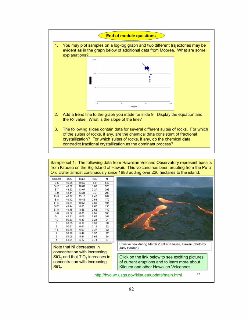
82
11
1. You may plot samples on a log-log graph and two different trajectories may be evident as in the graph below of additional data from Moorea. What are some explanations?
2. Add a trend line to the graph you made for slide 9. Display the equation and the R2 value. What is the slope of the line?
3. The following slides contain data for several different suites of rocks. For which of the suites of rocks, if any, are the chemical data consistent of fractional crystallization? For which suites of rocks, if any, do the chemical data contradict fractional crystallization as the dominant process?
1
10
100
1000
1 10 100 1000
Zn ( pp m)
End of module questions
12
Sample set 1: The following data from Hawaiian Volcano Observatory represent basalts from Kilauea on the Big Island of Hawaii. This volcano has been erupting from the Pu`uO`o crater almost continuously since 1983 adding over 220 hectares to the island.
Sample SiO2 MgO TiO2 NiS-5 46.68 19.52 1.8 542
S-15 46.82 18.87 1.86 525S-7 48.22 13.67 2.27 296S-9 48.41 13.34 2.3 293F-17 48.77 13.13 2.42 269S-8 49.12 10.45 2.53 170F-12 49.34 10.58 2.69 191S-25 49.44 8.85 2.67 130S-14 49.45 8.55 2.62 149S-3 49.62 8.85 2.55 168S-1 49.91 8.08 2.62 10410 50.53 6.33 3.23 946 50.55 6.19 3.31 908 50.61 6.61 3.12 92
F-5 50.76 6.09 3.37 822 50.99 5.42 3.57 725 51.06 5.44 3.65 681 51.24 5.12 3.74 87
Note that Ni decreases in concentration with increasing SiO2 and that TiO2 increases in concentration with increasing SiO2.
Effusive flow during March 2003 at Kilauea, Hawaii (photo by Judy Harden).
http://hvo.wr.usgs.gov/kilauea/update/main.html
Click on the link below to see exciting pictures of current eruptions and to learn more about Kilauea and other Hawaiian Volcanoes.
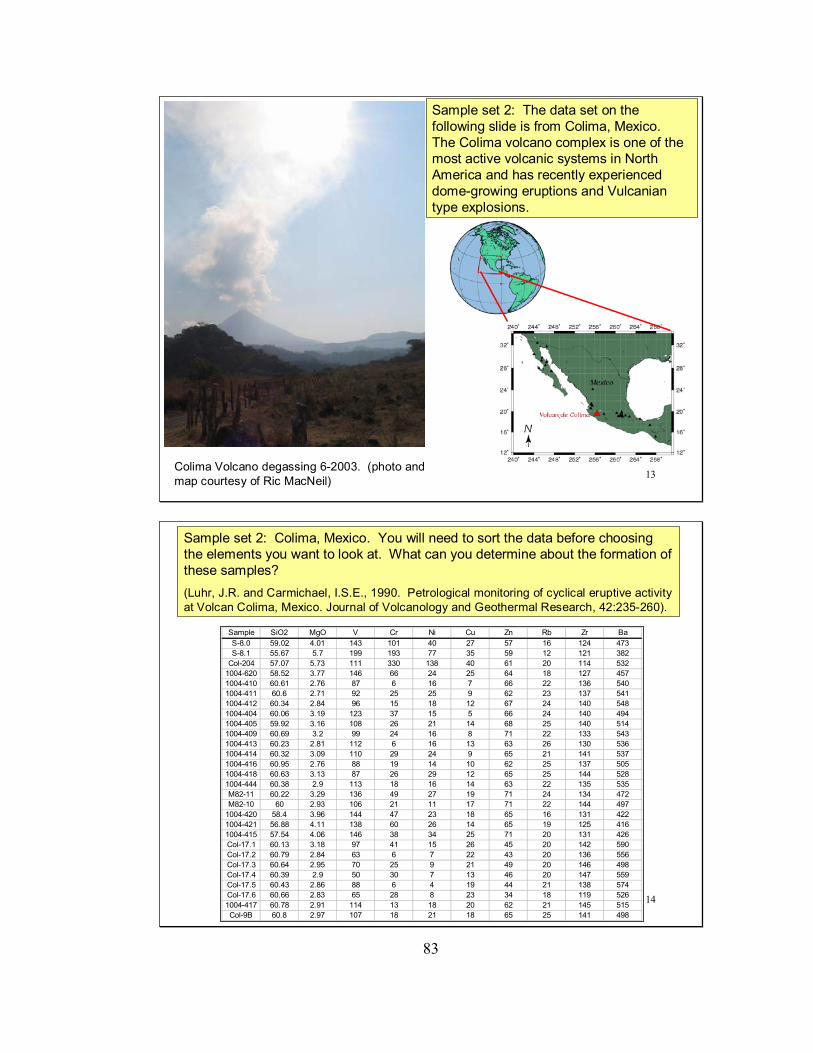
83
13
Sample set 2: The data set on the following slide is from Colima, Mexico. The Colima volcano complex is one of the most active volcanic systems in North America and has recently experienced dome-growing eruptions and Vulcaniantype explosions.
Colima Volcano degassing 6-2003. (photo and map courtesy of Ric MacNeil)
14
Sample set 2: Colima, Mexico. You will need to sort the data before choosing the elements you want to look at. What can you determine about the formation of these samples?(Luhr, J.R. and Carmichael, I.S.E., 1990. Petrological monitoring of cyclical eruptive activity at Volcan Colima, Mexico. Journal of Volcanology and Geothermal Research, 42:235-260).
Sample SiO2 MgO V Cr Ni Cu Zn Rb Zr BaS-8.0 59.02 4.01 143 101 40 27 57 16 124 473S-8.1 55.67 5.7 199 193 77 35 59 12 121 382
Col-204 57.07 5.73 111 330 138 40 61 20 114 5321004-620 58.52 3.77 146 66 24 25 64 18 127 4571004-410 60.61 2.76 87 6 16 7 66 22 136 5401004-411 60.6 2.71 92 25 25 9 62 23 137 5411004-412 60.34 2.84 96 15 18 12 67 24 140 5481004-404 60.06 3.19 123 37 15 5 66 24 140 4941004-405 59.92 3.16 108 26 21 14 68 25 140 5141004-409 60.69 3.2 99 24 16 8 71 22 133 5431004-413 60.23 2.81 112 6 16 13 63 26 130 5361004-414 60.32 3.09 110 29 24 9 65 21 141 5371004-416 60.95 2.76 88 19 14 10 62 25 137 5051004-418 60.63 3.13 87 26 29 12 65 25 144 5281004-444 60.38 2.9 113 18 16 14 63 22 135 535M82-11 60.22 3.29 136 49 27 19 71 24 134 472M82-10 60 2.93 106 21 11 17 71 22 144 497
1004-420 58.4 3.96 144 47 23 18 65 16 131 4221004-421 56.88 4.11 138 60 26 14 65 19 125 4161004-415 57.54 4.06 146 38 34 25 71 20 131 426Col-17.1 60.13 3.18 97 41 15 26 45 20 142 590Col-17.2 60.79 2.84 63 6 7 22 43 20 136 556Col-17.3 60.64 2.95 70 25 9 21 49 20 146 498Col-17.4 60.39 2.9 50 30 7 13 46 20 147 559Col-17.5 60.43 2.86 88 6 4 19 44 21 138 574Col-17.6 60.66 2.83 65 28 8 23 34 18 119 5261004-417 60.78 2.91 114 13 18 20 62 21 145 515Col-9B 60.8 2.97 107 18 21 18 65 25 141 498
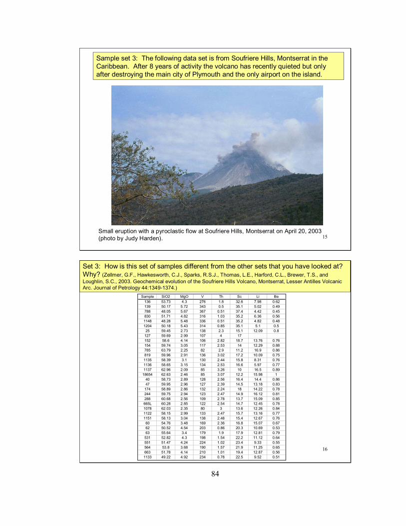
84
15
Sample set 3: The following data set is from Soufriere Hills, Montserrat in the Caribbean. After 8 years of activity the volcano has recently quieted but only after destroying the main city of Plymouth and the only airport on the island.
Small eruption with a pyroclastic flow at Soufriere Hills, Montserrat on April 20, 2003 (photo by Judy Harden).
16
Sample SiO2 MgO V Th Sc Li Be136 53.73 4.3 276 1.8 32.6 7.98 0.62139 50.17 5.72 343 0.5 35.1 5.02 0.49788 48.05 5.67 367 0.51 37.4 4.42 0.45830 51.71 4.82 316 1.03 35.2 6.36 0.561148 48.28 5.48 336 0.51 35.2 4.82 0.481204 50.18 5.43 314 0.85 35.1 5.1 0.525 59.45 2.73 138 2.3 15.1 12.09 0.8
127 59.69 2.99 107 4 17152 58.6 4.14 106 2.82 18.7 13.76 0.76154 59.74 3.05 117 2.53 14 12.29 0.88785 63.79 2.25 82 2.9 11.2 16.9 0.86819 59.96 2.91 136 3.02 17.2 10.09 0.751135 58.39 3.1 130 2.44 15.8 8.31 0.761136 58.65 3.15 134 2.53 16.6 5.97 0.771137 62.96 2.09 85 3.26 10 16.5 0.89
18654 62.63 2.46 85 3.07 12.2 15.98 140 58.73 2.89 128 2.56 16.4 14.4 0.8647 59.95 2.96 127 2.39 14.5 13.18 0.83
174 58.89 2.86 132 2.24 18 14.22 0.78244 59.75 2.94 123 2.47 14.9 16.12 0.81288 60.68 2.56 109 2.78 13.7 15.09 0.85665L 60.28 2.85 122 2.54 14.7 12.45 0.781078 62.03 2.35 80 3 13.6 12.26 0.841122 58.15 2.99 133 2.47 15.7 13.16 0.771151 58.13 3.04 138 2.48 15.4 12.67 0.7660 54.76 3.48 169 2.36 16.8 15.07 0.6762 50.52 4.54 203 0.86 20.3 10.69 0.5363 55.64 3.4 179 1.9 17.9 12.81 0.79
531 52.82 4.3 198 1.54 22.2 11.12 0.64551 51.47 4.24 224 1.02 23.4 9.33 0.55564 53.8 3.68 190 1.57 21.9 11.25 0.65663 51.78 4.14 210 1.01 19.4 12.87 0.561133 49.22 4.92 234 0.78 22.5 9.52 0.51
Set 3: How is this set of samples different from the other sets that you have looked at? Why? (Zellmer, G.F., Hawkesworth, C.J., Sparks, R.S.J., Thomas, L.E., Harford, C.L., Brewer, T.S., and Loughlin, S.C., 2003. Geochemical evolution of the Soufriere Hills Volcano, Montserrat, Lesser Antilles Volcanic Arc. Journal of Petrology 44:1349-1374.)

85
17
Geology related questions:
• What rock types or features of rocks do we see at the surface of the Earth that give us insight about the composition of the Earth’s mantle?
• What is fractional crystallization?• What is the difference between an incompatible and a compatible element?• What is the difference between a partition coefficient and a bulk partition
coefficient?• When plotting a suite of samples that are dominated by fractional
crystallization, what type of trend would you expect to see on a linear graph? On a logarithmic graph?
• Would a magma that undergoes fractional crystallization be depleted or enriched in incompatible elements?
Quantitative Literacy related questions:• What are the basic rules of logarithms?• What is forward modeling?• What is a weighted average?
Pre- and Post- module questions

86
Partial Melting Module JAH2A
1
We have gained much insight about the interior of the Earth since 1863. We now know that some Dante-like “seat of fires” does not exist and that volcanic eruptions occur when certain processes cause the rocks in the mantle to melt.
Students should work through module 1A and 1B (fractional crystallization) and have a basic understanding of phase diagrams before working through this module.
Mantle Processes2A – Partial Melting
Module JAH-2A
“Igneous rocks are those which have been ejected in a melted state, as from volcanic vents, or from fissures opened to some seat of fires within or below the earth’s crust.” –New Textbook of Geology (Dana, 1863)
2
PREVIEW
Slides 3-6 discuss the various known means of melting in the Earth’s interior: decreasing pressure, increasing temperature, and changing the composition of the mantle.
Slide 7 contains a simple animation of current ideas of how partial melting occurs and how the concentration of incompatible elements decreases as melting increases.
Slides 8-10 present a binary phase diagram and asks students to use the lever rule to calculate the percentage of a melt.
Slide 11 presents a calculation illustrating how much melting must occur to completely melt a mineral and change a phase.
Slide 12 – end-of-module questions.
See module JAH2B for an introduction of the Shaw equation and data sets to look for indications of partial melting.
This module is the first part of a set of two (JAH2A and JAH2B). JAH2A was developed to illustrate current ideas of how melting occurs within the mantle. JAH2B introduces ways to identify partial melting using geochemistry. It is highly recommended that each module be worked through for a better understanding of partial melting.

87
3
The Processes of Melting
Seismic data indicate that melting does not occur in the mantle under normal circumstances. Although various estimates have been calculated for the oceanic geothermal gradient, none of them approach the solidus of the mantle. Melting, therefore, is not a product of the geothermal gradient.
However, melting must occur or we would not have basalts erupted at the surface of the Earth.
There are only three known ways to cause melting in the mantle:
1. Lower the pressure2. Raise the temperature3. Change the composition
Before looking at samples, let’s take a look at these processes.
As with fractional crystallization, it is important to look at a suite of samples from the same source, rather than at a single sample, to identify partial melting.
4
Lowering pressure
Melting can occur by a decrease in pressure at a constant temperature. One way is to raise mantle rocks rapidly enough to minimize heat loss to the surroundings. Diverging plates are the prime location for this process to occur. Mantle material flows upward to fill in areas that have been vacated from erupting Mid-ocean ridge basalts (MORB).
This process is known as decompression melting. It occurs not only where plates are rifted apart. It also occurs at hot spots.
The material inside the area of the bold black lines is typically called “mush” by geologists. It consists of some solid and some melt.
Diagram after Wyllie, P.J., 1981. Plate tectonics and magma genesis. Geol. Rundsch, 70:128-153.
0
5
10
15
20
25
0 1000 2000 3000T (oC)
0
100
200
300
400
500
600
700
Dep
th (k
m)
Liquidus
solidus
Oceanic G
eotherm

88
5
Increasing temperatureMelting could occur if the mantle was heated beyond the normal geotherm by the decay of radioactive elements such as K, U, and Th. Radioactivity is the only known source of heat in the interior of the earth other than that from the primordial differentiation process.
The radioactive elements can produce only ~10-8 J g-1 a-1.
The specific heat of a typical rock is ~1 J g-1 deg-1.
With these values, it would take over 107 years for radioactivity in the mantle to increase the temperature in a mantle rock 1oC, making radioactivity an unlikely source for melt.
0
5
10
15
20
25
0 1000 2000 3000
T ( o C )
0
100
200
300
400
500
600
700
Liquidus
solidusOceanic G
eotherm
Diagram after Wyllie, P.J., 1981. Plate tectonics and magma genesis. Geol. Rundsch, 70:128-153.
6
Changing composition
Although the mantle is much more hydrated in subduction zones, amphibole and phlogopite have been found in mantle xenoliths. Water, therefore, is present in the mantle. Other fluid inclusions contain liquid CO2.
At high pressure, water can dramatically decrease the solidus temperature of the mantle. The water content of “normal” mantle is only ~0.1 weight %. In order to produce melting, however, additional volatiles need to be added to the mantle.
The following slide has a simple animation to show the process of changing the composition of the mantle.
Melts within the mantle are thought to be merely droplet sized.
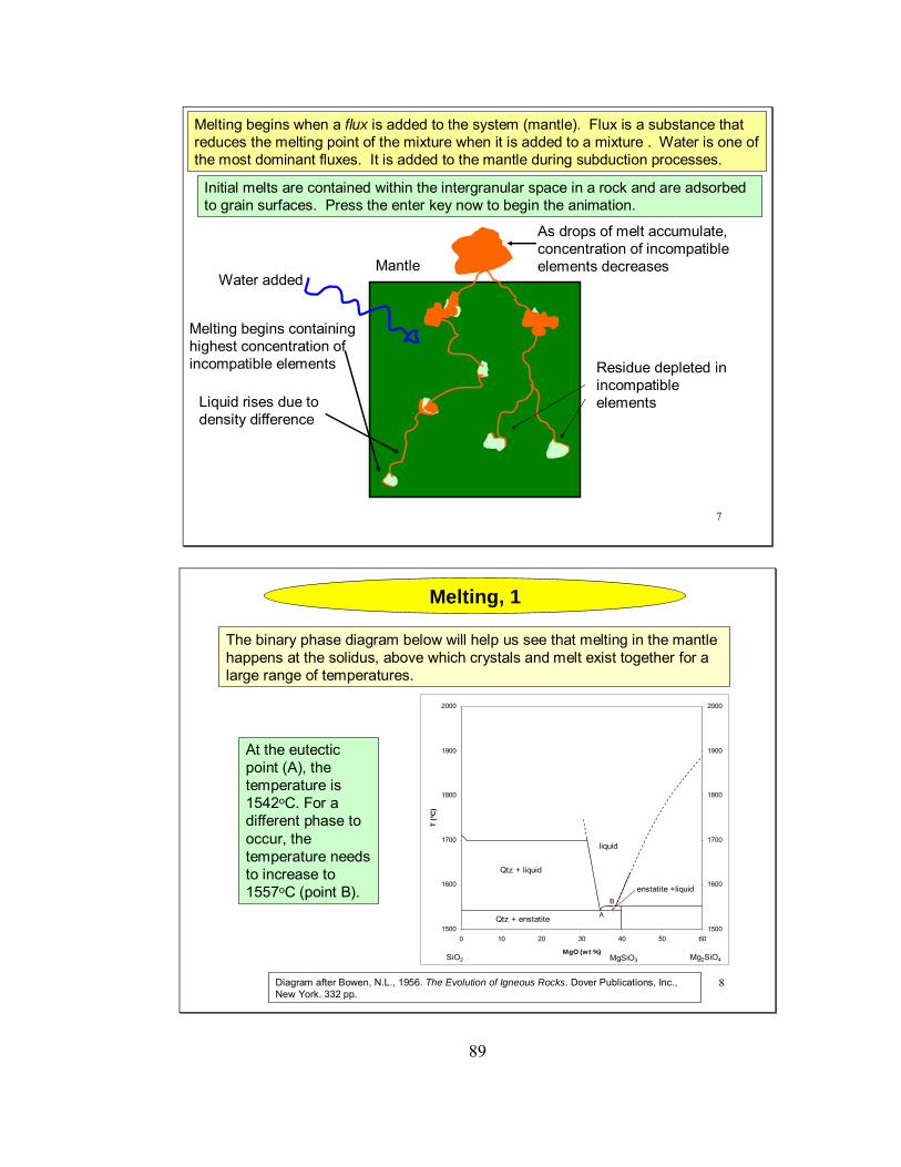
89
7
Melting begins when a flux is added to the system (mantle). Flux is a substance that reduces the melting point of the mixture when it is added to a mixture . Water is one of the most dominant fluxes. It is added to the mantle during subduction processes.
Initial melts are contained within the intergranular space in a rock and are adsorbed to grain surfaces. Press the enter key now to begin the animation.
Water added
Melting begins containing highest concentration of incompatible elements
Liquid rises due to density difference
As drops of melt accumulate, concentration of incompatible elements decreasesMantle
Residue depleted in incompatible elements
8
Melting, 1
The binary phase diagram below will help us see that melting in the mantle happens at the solidus, above which crystals and melt exist together for a large range of temperatures.
At the eutectic point (A), the temperature is 1542oC. For a different phase to occur, the temperature needs to increase to 1557oC (point B).
Diagram after Bowen, N.L., 1956. The Evolution of Igneous Rocks. Dover Publications, Inc., New York. 332 pp.
1500
1600
1700
1800
1900
2000
0 10 20 30 40 50 60
MgO (wt %)
T (o C
)
1500
1600
1700
1800
1900
2000
A
B
SiO2 Mg2SiO4MgSiO3
Qtz + liquid
Qtz + enstatite
liquid
enstatite +liquid
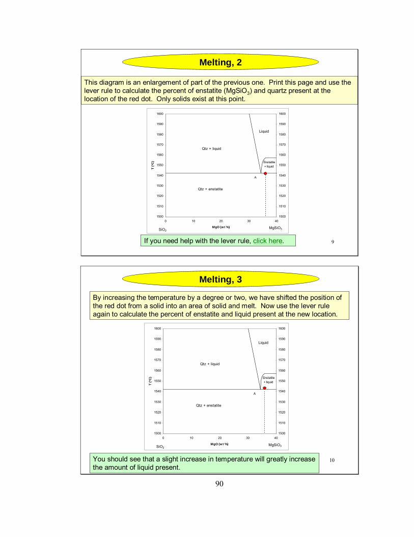
90
9
Melting, 2
This diagram is an enlargement of part of the previous one. Print this page and use the lever rule to calculate the percent of enstatite (MgSiO3) and quartz present at the location of the red dot. Only solids exist at this point.
If you need help with the lever rule, click here.
1500
1510
1520
1530
1540
1550
1560
1570
1580
1590
1600
0 10 20 30 40
MgO (wt %)
T (o C
)
1500
1510
1520
1530
1540
1550
1560
1570
1580
1590
1600
A
SiO2MgSiO3
Qtz + enstatite
Qtz + liquid
Enstatite + liquid
Liquid
10
Melting, 3
By increasing the temperature by a degree or two, we have shifted the position of the red dot from a solid into an area of solid and melt. Now use the lever rule again to calculate the percent of enstatite and liquid present at the new location.
You should see that a slight increase in temperature will greatly increase the amount of liquid present.
1500
1510
1520
1530
1540
1550
1560
1570
1580
1590
1600
0 10 20 30 40
MgO (wt %)
T (o C
)
1500
1510
1520
1530
1540
1550
1560
1570
1580
1590
1600
A
SiO2MgSiO3
Qtz + enstatite
Qtz + liquid
Enstatite + liquid
Liquid

91
11
Consider a mantle rock with a composition of 74% olivine, 15% orthopyroxene (opx), 10% clinopyroxene (cpx), and 1% spinel.
How much melting occurs?
From Bowen’s reaction series, we know that the pyroxenes will be the first to melt. If they melt equally at 50% cpx to 50% opx, how much melting must occur before all of the cpx is consumed and a phase change takes place?
We know that olivine forms as orthopyroxene melts, but the amount is small enough to disregard it in this calculation.
B C D2 % mineral % melt3 olivine 0.744 opx 0.15 0.15 cpx 0.1 0.16 spinel 0.017 ratio 1:18 % melt 0.2
A value larger than 20% melting is much higher than can occur according to experiments. This means that real-world melts do not get past the eutectic point and that an entire mineral phase will not melt.
12
1. How can we obtain mantle-derived samples such as the one described on slide 5? (ophiolites, dredge samples, xenoliths in basalts, xenoliths in kimberlites, possibly stony meteorites.)
2. Define the terms liquidus and solidus.
3. Determine the temperature in oF for the eutectic (point A) on slide 8.
4. Can hotspots be a means of adding heat to the mantle? (They can add heat to the mantle, but they are local perturbations and cannot produce all the basalt seen at the surface of the Earth.)
5. How do we know the mantle is predominantly solid? (Geophysical studies show that S-waves cannot propagate through a liquid; therefore, we know that the mantle is predominantly solid and the outer core is liquid.)
6. Using the values on slide 5, how long would it take for radioactivity in the mantle to increase the temperature in mantle rock 1oC? (1J/g deg / 10-8J/g a = 1 deg C / 107a)
End-of-module questions
Continue with partial melting module JAH2B.

92
Partial Melting Module JAH2B
1
The advances in geochemistry, geophysics, and volcanology have increased our understanding of the earth and the processes that shape and form it.
It is recommended that students work through JAH2A before working through this part of the module.
Mantle Processes2B – Partial Melting
Module JAH-2B
“The only way we can form any notion of what goes on at greater depths, is through volcanoes; they, therefore, deserve the careful study of any one who wishes to know the little that can be learned of the vast unknown region of the earth’s interior.” - First Book in Geology (Shaler, 1884)
2
PREVIEW
Slide 3 introduces the Shaw equation used for partial melting.
Slides 4-6 ask the students to develop a spreadsheet to calculate the Cl/Co ratio for given Dvalues and then to graph those values versus F to see the range of concentration of incompatible and compatible elements.
Slide 7 uses a spreadsheet mentioned in the Fractional Crystallization module (JAH1A) to calculate bulk partition coefficients.
Slides 8-9 ask students to use the Shaw equation to calculate and graph Cl/Co values for incompatible trace elements to see how concentrations vary with progressive melting.
Slides 10-11 offer some guidelines on what type of samples to choose, what elements to plot, and how to determine if partial melting has played a role in the formation of a given suite of rocks.
Slides 12-17 end-of-module questions and related data.
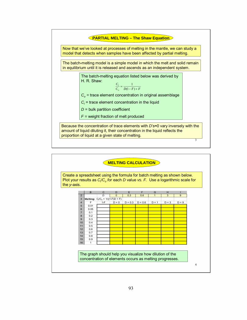
93
3
Because the concentration of trace elements with D’s≈0 vary inversely with the amount of liquid diluting it, their concentration in the liquid reflects the proportion of liquid at a given state of melting.
The batch-melting model is a simple model in which the melt and solid remain in equilibrium until it is released and ascends as an independent system.
The batch-melting equation listed below was derived by H. R. Shaw:
Co = trace element concentration in original assemblage
Cl = trace element concentration in the liquid
D = bulk partition coefficient
F = weight fraction of melt produced
FFDCC
o
l
+−=
)1(1
PARTIAL MELTING – The Shaw Equation
Now that we’ve looked at processes of melting in the mantle, we can study a model that detects when samples have been affected by partial melting.
4
The graph should help you visualize how dilution of the concentration of elements occurs as melting progresses.
Create a spreadsheet using the formula for batch melting as shown below. Plot your results as Cl/Co for each D value vs. F. Use a logarithmic scale for the y-axis.
B C D E F G H I2 D 0 0.3 0.6 1 3 93 Melting: Cl/Co = 1/((1-F)D + F)4 F 1-F D = 0 D = 0.3 D = 0.6 D = 1 D = 3 D = 95 0.016 0.057 0.18 0.29 0.310 0.411 0.512 0.613 0.714 0.815 0.916 1
MELTING CALCULATION

94
5When D >> 1, the concentration of compatible elements in the melt show only small ranges in abundance during initial melting.
For small values of F (low degrees of melting), the concentration of highly incompatible elements (D << 1) varies greatly.
The highly incompatible elements concentrate in the first few drops of melt and become progressively more dilute as F increases.
PARTIAL MELTING
MELTING
0.1
1.0
10.0
100.0
0 0.2 0.4 0.6 0.8 1
F
Cl/C
o
D = 0
D = 0.3
D = 0.6
D = 1
D = 3
D = 9
6Let’s see how this technique works.
If we know the concentration of a trace element in a magma (Cl) and D, we can use the Shaw equation to calculate Co enabling us to characterize and constrain the source region of magmas. When F approaches zero, the equation reduces to:
DCC
o
l 1=
By knowing the concentration of a highly incompatible element (D 0) in the magma and the source rock, we can calculate F, the fraction of partial melt produced.
FCC
o
l 1=
PARTIAL MELTING
Only those elements with D’s <<1 show a wide range in abundance for a given range of F. For example, the maximum enrichment for an element with D = 0.01 is 100 while an element with D = 0.3 the maximum enrichment is 3.3.

95
7
http://earthref.org/GERM/index.html?main.htm
Suppose we have a sample of basalt derived from melting in the mantle with a composition of 70% olivine, 17% orthopyroxene (opx), 12% clinopyroxene(cpx), and 1% spinel. Use the spreadsheet you created in slide 7 of module 1A and KD values for Rb and Li from the Geochemical Earth Reference Model (GERM) website listed below to calculate D for each element.
You should discover that Rb is highly incompatible and that Li is only slightly more compatible than Rb (moderately incompatible).
Now we can calculate Cl/Co for different F values.
COMPATIBILITY
B C D2 X K D
3 Olivine 0.7 0.044 opx 0.17 0.00065 cpx 0.12 0.016 spinel 0.01 078 DRb =
B C D2 X K D
3 Olivine 0.7 0.354 opx 0.17 0.265 cpx 0.126 spinel 0.0178 DLi =
8
Using the Shaw equation, calculate the Cl/Co ratio for Rb and Li. Add another column to calculate the Rb/Li ratio.
After completing the spreadsheet, plot the Cl/Co ratios for the two elements vs F on a linear graph with arithmetic scales on both axes.
B C D E2 Rb Li3 D 0.03 0.2945 F Rbl/Rbo Lil/Lio Rb/Li6 0.057 0.18 0.159 0.210 0.2511 0.312 0.413 0.514 0.615 0.716 0.817 0.918 1
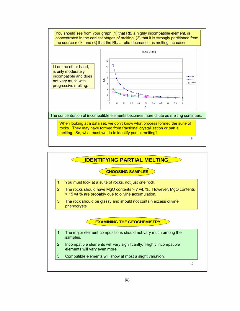
96
9
You should see from your graph (1) that Rb, a highly incompatible element, is concentrated in the earliest stages of melting; (2) that it is strongly partitioned from the source rock; and (3) that the Rb/Li ratio decreases as melting increases.
When looking at a data set, we don’t know what process formed the suite of rocks. They may have formed from fractional crystallization or partial melting. So, what must we do to identify partial melting?
The concentration of incompatible elements becomes more dilute as melting continues.
Partial Melting
0
2
4
6
8
10
12
14
0 0.1 0.2 0.3 0.4 0.5 0.6 0.7 0.8 0.9 1
FC
l/Co
Rb
Li
Rb/Li
Li on the other hand, is only moderately incompatible and does not vary much with progressive melting.
10
1. You must look at a suite of rocks, not just one rock.
2. The rocks should have MgO contents > 7 wt. %. However, MgO contents > 15 wt % are probably due to olivine accumulation.
3. The rock should be glassy and should not contain excess olivine phenocrysts.
CHOOSING SAMPLES
1. The major element compositions should not vary much among the samples.
2. Incompatible elements will vary significantly. Highly incompatible elements will vary even more.
3. Compatible elements will show at most a slight variation.
EXAMINING THE GEOCHEMISTRY
IDENTIFYING PARTIAL MELTING

97
11
A steeply-sloped, tight linear trend (A) indicates partial melting as a dominant process while a shallower slope with a more scattered trend (B) indicates some other process such as fractional crystallization (but not necessarily).
EXAMINING THE GRAPHS
Because the concentration of highly incompatible elements has such a large range, and moderately incompatible elements vary only slightly, a plot on a linear graph of the ratio of a highly incompatible element to a moderately incompatible element vsthe moderately incompatible element is best (Example: Be/Li vs. Be)
What elements are the best to plot?
0
2
4
6
8
10
12
14
0 20 40 60 80 100 120
highly incompatible
high
ly in
com
patib
le/m
od. i
ncom
patib
le
0
1
2
3
4
5
6
0 10 20 30 40 50
highly incompatiblehi
ghly
inco
mpa
tible
/mod
. inc
ompa
tibleA B
12
1. As F approaches 1, what can we say about the Cl/Co ratio in the Shaw equation? (The concentration of every trace element in the melt equals theconcentration in the source rock, it approaches 1.)
2. Make plots of the data from various settings on the following slides (You will need to use the spreadsheet and rock compositions from slide 7 and KD values from the GERM website to calculate D values so that you will know which trace elements to plot). Which suite of rocks, if any, indicates that partial melting was a dominant process of formation.
3. After plotting all the data, create a spreadsheet like the example below to calculate F for each sample in any suite of rocks that appears to have been formed from partial melting. Be sure to use element(s) with a Dvalue close to zero (see slide 6):
End-of-module questions
B C D2 C o
3 0.02 ppm45 C l F6 0.205 107 0.207 108 0.257 89 0.257 8
10 0.164 1211 0.242 812 0.382 5
Co for Be ~ 0.01
Co for Ba ~ 1.1
Co for Li ~ 1.9
Co for Zr ~ 9.0
Co for Y ~ 4.0
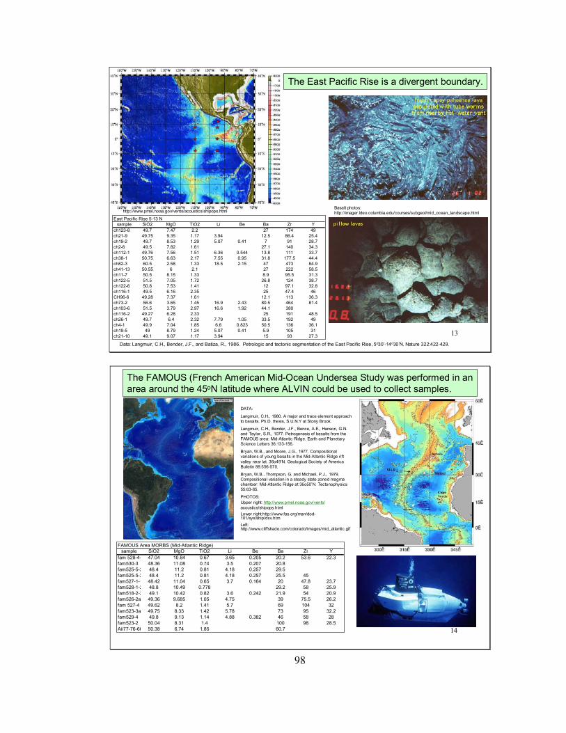
98
13
East Pacific Rise 5-13 Nsample SiO2 MgO TiO2 Li Be Ba Zr Y
ch123-8 49.7 7.47 2.2 27 174 49ch21-9 49.75 9.35 1.17 3.94 12.5 86.4 25.4ch19-2 49.7 8.53 1.29 5.07 0.41 7 91 28.7ch2-6 49.5 7.82 1.61 27.1 140 34.3ch112-1 49.76 7.56 1.51 6.36 0.544 13.8 111 33.7ch38-1 50.75 6.63 2.17 7.55 0.95 31.8 177.5 44.4ch82-3 60.5 2.58 1.33 18.5 2.15 47 473 84.9ch41-13 50.55 6 2.1 27 222 58.5ch11-7 50.5 8.15 1.33 8.9 95.5 31.3ch122-5 51.5 7.05 1.72 26.8 124 38.7ch122-6 50.8 7.53 1.41 12 97.1 32.8ch116-1 49.5 6.16 2.35 25 47.4 46CH96-6 49.28 7.37 1.61 12.1 113 36.3ch73-2 56.6 3.65 1.45 16.9 2.43 80.5 464 81.4ch103-6 51.5 3.79 2.97 16.6 1.92 44.1 380ch116-2 49.27 6.28 2.33 25 191 48.5ch26-1 49.7 6.4 2.32 7.79 1.05 33.5 192 49ch4-1 49.9 7.04 1.85 6.6 0.823 50.5 136 36.1ch19-5 49 8.79 1.24 5.07 0.41 5.9 105 31ch21-10 49.1 9.07 1.17 3.94 15 93 27.3
The East Pacific Rise is a divergent boundary.
Data: Langmuir, C.H., Bender, J.F., and Batiza, R., 1986. Petrologic and tectonic segmentation of the East Pacific Rise, 5o30’-14o30’N. Nature 322:422-429.
http://www.pmel.noaa.gov/vents/acoustics/shipops.htmlBasalt photos:http://imager.ldeo.columbia.edu/courses/subgeol/mid_ocean_landscape.html
14
FAMOUS Area MORBS (Mid-Atlantic Ridge)sample SiO2 MgO TiO2 Li Be Ba Zr Y
fam 528-4- 47.04 10.84 0.67 3.65 0.205 20.2 53.6 22.3fam530-3 48.36 11.08 0.74 3.5 0.207 20.8fam525-5-2 48.4 11.2 0.81 4.18 0.257 29.5fam525-5-2 48.4 11.2 0.81 4.18 0.257 25.5 45fam527-1-1 48.42 11.04 0.65 3.7 0.164 20 47.8 23.7fam528-1-2 48.8 10.49 0.778 29.2 58 25.9fam518-2-2 49.1 10.42 0.82 3.6 0.242 21.9 54 20.9fam526-2a 49.36 9.685 1.05 4.75 39 75.5 26.2fam 527-4 49.62 8.2 1.41 5.7 69 104 32fam523-3a 49.75 8.33 1.42 5.78 73 95 32.2fam529-4 49.8 9.13 1.14 4.88 0.382 46 58 28fam523-2 50.04 8.31 1.4 100 98 28.5Aii77-76-66 50.38 6.74 1.85 60.7
The FAMOUS (French American Mid-Ocean Undersea Study was performed in an area around the 45oN latitude where ALVIN could be used to collect samples.
DATA:
Langmuir, C.H., 1980. A major and trace element approach to basalts. Ph.D. thesis, S.U.N.Y at Stony Brook.
Langmuir, C.H., Bender, J.F., Bence, A.E., Hanson, G.N. and Taylor, S.R., 1077. Petrogenesis of basalts from the FAMOUS area: Mid-Atlantic Ridge. Earth and Planetary Science Letters 36:133-156.
Bryan, W.B., and Moore, J.G., 1977. Compositional variations of young basalts in the Mid-Atlantic Ridge rift valley near lat. 36o49’N. Geological Society of America Bulletin 88:556-570.
Bryan, W.B., Thompson, G. and Michael, P.J., 1979. Compositional variation in a steady state zoned magma chamber: Mid-Atlantic Ridge at 36o50’N. Tectonophysics55:63-85.
PHOTOS:Upper right: http://www.pmel.noaa.gov/vents/acoustics/shipops.htmlLower right:http://www.fas.org/man/dod-101/sys/ship/dsv.htm Left: http://www.cliffshade.com/colorado/images/mid_atlantic.gif

99
15
Juan De Fuca Ridgesample SiO2 MgO TiO2 Li Be Ba Zr Y
jfd01-04 50.81 3.417 2.997 16.75 1.66 47.45 403 101jfc02-01 50.6 5.08 2.49 10.5 1.2 42 294 75aii84-wf7-4 49.69 6.05 2.12 26.6 205.5 57.09aii84-wf12- 49.48 6.96 1.82 7.52 0.586 16.7 127.8 42aii84-wf13- 49.52 7.71 1.44 6.1 0.412 14.5 95.6 33.91461-7r 49.74 6.9 1.83 17.6 135.1 42.21411-b1 48.86 7.45 1.46 5.27 0.498 27.7 101 311410-2a 50 8.6 1.23 13 81 28.7jfd-2 50.14 6.75 1.86 7.8 0.65 22 159 48JFD03-03 50.91 7.3 1.8 20 129 421405-B5 49.49 8 1.38 9.63 95.1 34.81415-B5-2 49.12 7.54 1.59 14 109 38.5JFD02-01 50.9 7.2 1.77 17 123 40.3JFD11-02 48.3 7.9 1.41 28 104 30aii84-WF-2 50.9 7 1.8 20 147 45.51406-2B-7 49.6 8.63 1.16 13 76 28.51410-3B 49.4 8.6 1.23 13 88 29.5
The Juan de Fuca ridge is a divergent boundary off the coast of western Canada.
Kappel, E., 1985. Evidence for volcanic episodicity and a non-steady state rift valley. Ph.D. thesis, Columbia University.
http://www.pgc.nrcan.gc.ca/geodyn/french/cascadia.htm
http://www.pmel.noaa.gov/pubs/outstand/embl2063/images/plate01.jpg
http://www.bcadventure.com/adventure/frontier/physio/tectonic.htm
http://www.bcadventure.com/adventure/frontier/physio/bcplate.gif
16
Society IslandsSample SiO2 MgO TiO2 Li Be Ba Zr Y101287 4.5 1.0101288 6.2 1.1101211 2.90 6.3 1.0 513.82101198 52.1 4.3 2.83 9.3 2.7
MAO-113 3.21 6.6 1.5 355.25MAO 65 3.6 1.5 433.2273-204 45.7 12.5 2.76 5.9 1.3 410.39
MHT-101 44.2 15.7 3.32 3.7 1.1 304.58MHT-155 44.8 14.6 3.56 4.3 1.2 344.85
Ta3F 50.7 7.7 3.08 5.4 0.9 506.35Ta8b 46.8 13.0 3.05 5.1 1.0 429.58
74-422 42.8 10.7 3.74 5.8 1.1 409.1674-437 46.5 9.2 7.0 2.1 621.41
The Society Islands, French Polynesia, were formed by a hot spot like the islands of Hawaii.
White, W.M.,
Harden, J.A., 2004. Light Element and Lithium Isotope Signatures of the EM II Reservoir: The Society Islands, French Polynesia: Geochemical Results and an Educational Application. M.S. thesis, University of South Florida.

100
17
N
Moorea is the third youngest island in the Society Chain.
MooreaSample SiO2 MgO TiO2 Li Be Ba Zr Y
M01FISH2D 46.0 14.5 2.70 4.9 1.2 78M01FISH A 45.4 13.3 2.93 5.1 1.2 211
M01T1A 45.8 11.2 2.93 5.4 1.0 270M01FISH2B 46.0 13.4 2.89 4.7 1.5 222M01FISHB1 46.2 11.8 3.08 5.8 1.5 374M01FISH2A 46.2 12.4 3.03 6.9 1.8 327M03PK19N 46.4 14.1 2.74 5.8 0.7 320
M01B2C 46.8 13.5 3.00 5.9 1.4 300M01AIR 1A 46.9 11.4 3.24 3.2 1.4 296
M03020 47.0 14.1 2.56 6.9 1.1 309M03011 47.2 14.1 2.62 12.3 2.9 298M03010 47.6 14.5 2.74 6.7 1.1 244M01B1A 47.6 7.9 3.18 6.6 1.0 268M01QB 49.0 9.2 2.59 11.3 2.8 251M01T2A 49.0 8.9 3.34 7.8 1.8 353M01QA 49.4 8.4 2.71 13.2 3.0 249
To the right are thin sections of basalts from the island. The middle photo is of a xenolith.
Harden, J.A., 2004. Light Element and Lithium Isotope Signatures of the EM II Reservoir: The Society Islands, French Polynesia: Geochemical Results and an Educational Application. M.S. thesis, University of South Florida.
Top Related