Lexical Analysis of US Political Speeches*

Jacques SavoyComputer Science Department, University of Neuchatel, Switzerland

ABSTRACT

This article describes a US political corpus comprising 245 speeches given by senatorsJohn McCain and Barack Obama during the years 2007–2008. We present the maincharacteristics of this collection and compare the common English words most frequentlyused by these political leaders with ordinary usage (Brown corpus). We then discuss andcompare certain metrics capable of extracting terms best characterizing a given subset ofthe entire text corpus. Terms overused and underused by both candidates during the lastUS presidential election are determined and analysed from both a statistical and dynamicperspective.

1. INTRODUCTION

The presidential election was the major political event in the UnitedStates in 2008. During this campaign the candidates (or their speech-writers) wrote various speeches that would hopefully convince undecidedvoters, to encourage their supporters and to make obvious that they werethe best candidates for the job. The words and expressions used in theirdiscourses were therefore not chosen randomly but rather to reflect thesevarious objectives. Since the candidates’ speeches targeted the sameelection, and they expressed their views during the same period andconcerned the same goals and related topics, we were thus able tocompare the speeches more objectively than say various literary worksselected from different periods, styles (e.g. tragedies, novels) and genres(prose vs. poetry). We must, however, recognize that in politics the

*Address correspondence to: Jacques Savoy, Computer Science Department, Universityof Neuchatel, rue Emile Argand 11, 2009 Neuchatel, Switzerland. Tel: þ41 32 718 2700.Fax: þ41 32 718 2701. E-mail: Jacques.Savoy@unine.ch

Published in Journal of Quantitative Linguistics 17, issue 2, 123-141, 2010 which should be used for any reference to this work

1

official version is usually the spoken one. But we can consider that thewritten version, usually available on each candidate’s website, revealsaccurately the speaker’s real intent. Also, these freely available textsusually contain few spelling errors and abbreviations, which from theinformation technology point of view render their use without realproblems. Finally, from the perspective of interpreting and verifyingresults, we deem it easier to work with political speeches rather than withtexts from more technical domains.Using words extracted from these speeches, our objective is to define

the various terms that can characterize well each subset of our overall USpolitical corpus. These subsets could be defined according to date (2007vs. 2008), author (J. McCain vs. B. Obama), topic (e.g. energy vs. foreignpolicy), form (spoken vs. written), or target audience (e.g. business vs.academic). For the purposes of this article, we limit ourselves to onlydistinguishing the author and the date (month and year).The rest of this paper is organized as follows. Section 2 presents a brief

overview of related work in political discourse analyses. Section 3provides an overview of our US political corpus while Section 4 discussescertain metrics used to define and weight the terms best characterizing thedifferences between two (or more) sets of documents (corpus partitions).Section 5 describes the main differences revealed through comparing thetwo candidates, while Section 6 shows their differences from a dynamicperspective. Section 7 displays how we follow the importance of a giventopic throughout the entire campaign, on a month-by-month basis.Finally, Section 8 contains some conclusions.

2. RELATED WORK

In our analysis of political corpora and lexical analysis, we pay tribute tothe work done by Labbe and Moniere (2003) in comparing the threesources of government speeches (e.g., speeches from the Throne[Canada], inaugural speeches [Quebec] and investiture speeches [France]).The advantage of their work is that it covers documents written in theFrench language, over a relatively long period of time (50 years, from1945 to 2000) and makes it possible to compare political discourses fromthese countries. This corpus however only consists of governmentspeeches, and thus they were not necessarily written for electoralpurposes. We can expect certain differences between a prime minister

2

in charge of a government and one who is hoping to be elected (Herman,1974). Even though these government speeches express the ideas ofdistinct political parties, according to Labbe and Moniere (2003) theytended to be more similar than expected, mainly due to institutionalconstraints. As such, continuity clearly imposes stronger constraints thanpolitical cleavages. They did note, however, a certain trend towardslonger speeches (perhaps related to television broadcasting and thecomplexity of the underlying questions).Measuring lexical richness objectively is a complex problem especially

given that a well-grounded operational definition does not exist. To do sowe need to take into account the number of distinct words, vocabularydiversity and expansion over time, lexical specificity, etc. (Baayen, 2008).According to Labbe and Moniere (2003), the reason for vocabularyincreases cannot be attributed to a single and well-defined event, but maytake place when a strong personality takes power, such as that of PrimeMinister Trudeau (1968–72) in Canada, or Rocard (1988) and Beregovoy(1992) in France.There are, of course, other pertinent questions related to our research.

One might wish to discover the name of the actual speechwriter behindeach discourse (as, for example, T. Sorensen behind President Kennedy;Carpenter & Seltzer, 1970). We might also compute textual distancesbetween speeches, sets of speeches or political leaders (based on theirspeeches) to measure the relative distance between them (Labbe, 2007).Based on this information, we could then draw a political map showingthe various political leaders according to their respective similarities(Labbe & Moniere, 2003).

3. OUR US POLITICAL CORPUS

This US political corpus contains speeches we downloaded from the twocandidates’ official websites. For each speech, we added a few meta-tagsto store document information (e.g. date, location, title), and we alsocleaned them up by replacing certain UTF-8 coding system punctuationmarks with their corresponding ASCII code symbol. This involvedreplacing single (‘’) or double quotation marks (‘‘’’), with the (0) or (00)symbols, and the removal of diacritics found in some certain words (e.g.‘‘naıve’’). To improve matching between surface forms we also replacedupper-case letters by their corresponding lower-case, except for those

3

words written only with capital letters (e.g. ‘‘US’’, ‘‘FEMA’’ [FederalEmergency Management Agency]).On the other hand, we did not try to normalize various word forms

referring to the same entity such as ‘‘US’’, ‘‘United States’’, ‘‘UnitedStates of America’’, or ‘‘USA’’ (‘‘America’’, ‘‘our country’’ etc.). Weassume that the authors maintain the same form across the two years andthat they will use the same spelling. This assumption is reasonable, giventhat both candidates would follow the same objectives and their speecheswould be extracted from the same time period.

3.1 Overall statistics

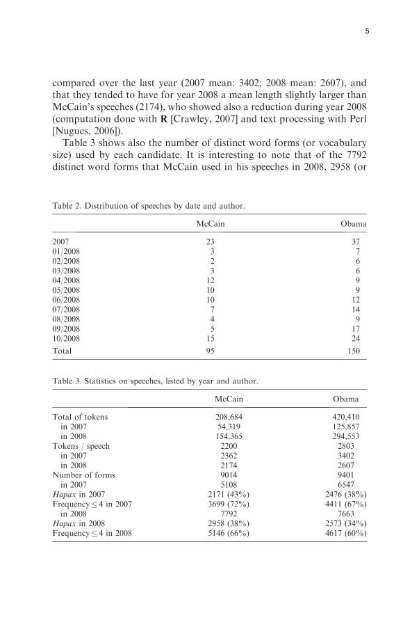
Obama’s speeches were downloaded from www.barackobama.com,beginning with the first on 10 February 2007 and ending with that on30 October 2008 (Table 1 indicated the main dates of this election). Intotal our corpus contains 150 speeches (37 in 2007, 113 in 2008), fora total data size of 2.3 Mb (0.7 Mb for 2007, 1.6 Mb for 2008). Forthe Republican Party’s speeches, we downloaded them from www.johnmccain.com beginning on 25 April 25 2007. This second subsetcontains 95 speeches (23 for 2007, 72 for 2008), for a total of 1.2 Mb (0.3Mb for 2007, 0.9 Mb for 2008).The data listed in Table 2 shows that McCain gave fewer speeches than

Obama (95 vs. 150). Their distribution across the entire period showsthat Obama tended to give more speeches, except for the months of Apriland May 2008.From inspecting the number of word tokens per author and date (see

Table 3), we see that B. Obama reduced the volume of his speeches

Table 1. Main events during the latest US presidential campaign.

10 February 2007: Senator Barack Obama (IL) announced his candidacy for President25 April 2007: Senator John McCain (AZ) announced his intention to run for President5 February 2008: Super Tuesday7 June 2008: Hillary Clinton ended her campaign23 August 2008: John Biden nominee as Vice-President (D)25–28 August 2008: Democrat convention30 August 2008: Sarah Palin nominee as Vice-President (R)1–4 September 2008: Republican convention1 September 2008: Official campaign starts4 November 2008: Election day20 January 2009: Inauguration day

4

compared over the last year (2007 mean: 3402; 2008 mean: 2607), andthat they tended to have for year 2008 a mean length slightly larger thanMcCain’s speeches (2174), who showed also a reduction during year 2008(computation done with R [Crawley, 2007] and text processing with Perl[Nugues, 2006]).Table 3 shows also the number of distinct word forms (or vocabulary

size) used by each candidate. It is interesting to note that of the 7792distinct word forms that McCain used in his speeches in 2008, 2958 (or

Table 2. Distribution of speeches by date and author.

McCain Obama

2007 23 3701/2008 3 702/2008 2 603/2008 3 604/2008 12 905/2008 10 906/2008 10 1207/2008 7 1408/2008 4 909/2008 5 1710/2008 15 24

Total 95 150

Table 3. Statistics on speeches, listed by year and author.

McCain Obama

Total of tokens 208,684 420,410in 2007 54,319 125,857in 2008 154,365 294,553

Tokens / speech 2200 2803in 2007 2362 3402in 2008 2174 2607

Number of forms 9014 9401in 2007 5108 6547

Hapax in 2007 2171 (43%) 2476 (38%)Frequency� 4 in 2007 3699 (72%) 4411 (67%)in 2008 7792 7663

Hapax in 2008 2958 (38%) 2573 (34%)Frequency� 4 in 2008 5146 (66%) 4617 (60%)

5

38%) word forms were used only once (a phenomenon known as hapax).Words used four times or less represent a rather large proportion, namely66.1% of the total (or 5146 word forms). An analysis of Obama’svocabulary reveals a similar pattern. Also noteworthy is that even thoughMcCain gave fewer speeches than Obama in 2008 (95 vs. 150), hisvocabulary tended to have a similar size (9014 vs. 9401).

3.2 Most frequent words

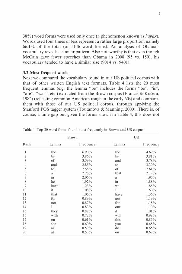
Next we compared the vocabulary found in our US political corpus withthat of other written English text formats. Table 4 lists the 20 mostfrequent lemmas (e.g. the lemma ‘‘be’’ includes the forms ‘‘be’’, ‘‘is’’,‘‘are’’, ‘‘was’’, etc.) extracted from the Brown corpus (Francis & Kucera,1982) (reflecting common American usage in the early 60s) and comparesthem with those of our US political corpus, through applying theStanford POS tagger system (Toutanova & Manning, 2000). There is, ofcourse, a time gap but given the forms shown in Table 4, this does not

Table 4. Top 20 word forms found most frequently in Brown and US corpus.

Brown US

Rank Lemma Frequency Lemma Frequency

1 the 6.90% the 4.69%2 be 3.86% be 3.81%3 of 3.59% and 3.78%4 and 2.85% to 3.30%5 to 2.58% of 2.61%6 a 2.28% that 2.17%7 in 2.06% a 1.95%8 he 1.92% in 1.88%9 have 1.23% we 1.85%

10 it 1.08% I 1.50%11 that 1.05% have 1.36%12 for 0.89% not 1.19%13 not 0.87% for 1.18%14 I 0.83% our 1.10%15 they 0.82% it 1.01%16 with 0.72% will 0.98%17 on 0.61% this 0.85%18 she 0.60% you 0.68%19 as 0.59% do 0.65%20 at 0.53% on 0.62%

6

seem to play a really significant role and would thus not invalidate anycomparisons.From Table 4 it can be seen that ‘‘the’’ tends to occur more frequently

in ordinary language (6.9%) than in political speeches (4.69%). What ismore interesting is the conjunction ‘‘that’’ which ranks 6th in our USpolitical speeches but only 11th in the Brown corpus. This tends toindicate that politicians tend to produce longer sentences with morecomplex syntax, reflecting a need to be more precise or to explain certainproblems in depth. Political speeches are often characterized by thefrequent use of the pronoun ‘‘we’’ (ranked 9th compared with 23rd in theBrown corpus). The verb ‘‘will’’ shows a similar pattern (16th vs. 35th inthe Brown corpus). The pronoun ‘‘he’’, however (8th in the Browncorpus), is used less in our US corpus, where it is ranked 44th. Thedifference is even greater for the pronoun ‘‘she’’ (18th vs. 208th).Applying the Wilcoxon matched-pairs signed-ranks test (Conover, 1971)on data depicted in Table 4, we can verify whether both rankings reflect asimilar words usage. In the current case, we must reject this hypothesis(significance level a¼ 0.05, p-value5 0.001).

4. METRICS

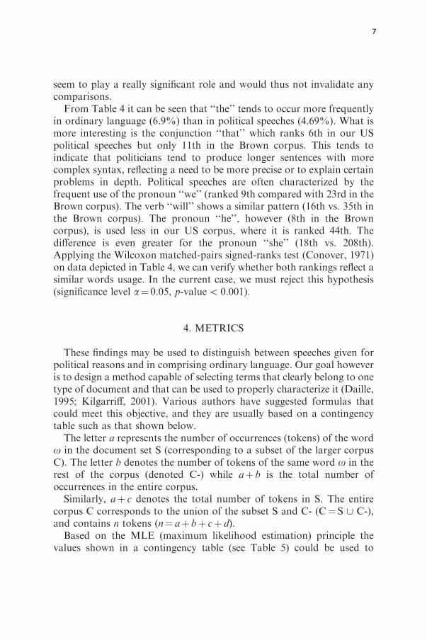
These findings may be used to distinguish between speeches given forpolitical reasons and in comprising ordinary language. Our goal howeveris to design a method capable of selecting terms that clearly belong to onetype of document and that can be used to properly characterize it (Daille,1995; Kilgarriff, 2001). Various authors have suggested formulas thatcould meet this objective, and they are usually based on a contingencytable such as that shown below.The letter a represents the number of occurrences (tokens) of the word

o in the document set S (corresponding to a subset of the larger corpusC). The letter b denotes the number of tokens of the same word o in therest of the corpus (denoted C-) while aþ b is the total number ofoccurrences in the entire corpus.Similarly, aþ c denotes the total number of tokens in S. The entire

corpus C corresponds to the union of the subset S and C- (C¼ S [ C-),and contains n tokens (n¼ aþ bþ cþ d).Based on the MLE (maximum likelihood estimation) principle the

values shown in a contingency table (see Table 5) could be used to

7

estimate various probabilities. For example we might calculate theprobability of the occurrence of the word o in the entire corpus C asProb(o)¼ (aþ b)/n or the probability of finding in C a word belonging tothe set S as Prob(S)¼ (aþ c)/n.As a first approach in determining whether a given word o could be

used to describe the subset S quite adequately, we might consider twoevents. First we could estimate the probability of selecting the word o inthe entire corpus C (Prob(o)¼ (aþ b)/n). On the other hand, theprobability of selecting a word in C belonging to the set S could beestimated by Prob(S)¼ (aþ c)/n. Then if we consider selecting from C anoccurrence of the word o belonging to the set S, we could estimate thisprobability using Prob(o \ S)¼ a/n. However we could also assume thatthe joint event (o \ S) would be independent (by chance only) of bothevents (o and S), which in turn would lead to another estimate,Prob(o) � Prob(S).To comparing these two estimates we would use the approach adopted

by the mutual information (MI) measure (Church & Hanks, 1990),defined as:

Iðo; SÞ ¼ log2Probðo \ SÞ

ProbðoÞ � ProbðSÞ

� �¼ log2

a

ðaþ bÞ�

n

ðaþ cÞ

� �ð1Þ

When the two estimates are close (I(o, S) � 0), this means there is noreal association between the word o and the set S. In such cases, theoccurrences of word o in S can be explained simply by chance. When theword o is used more often within S, then a positive association developsbetween them and we could find that Prob(o \ S)4Prob(o) � Prob(S),resulting in I(o; S)4 0. Finally, if Prob(o \ S)55Prob(o) � Prob(S),this indicates that the two events are complementary and thus I(o;S)5 0. An example using this metric is given in Table 6 illustrating howthe word ‘‘IT’’ is distributed in Obama’s speeches in 2008 and in the restof our US corpus.

Table 5. Example of a contingency table.

S C-

o a b aþ bNot o c d cþ d

aþ c bþ d n¼ aþ bþ cþ d

8

From data depicted in Table 6, we could estimate directly theprobability Prob(o \ S) as 1/629,094 that corresponds to the numeratorof Equation (1). On the other hand, we may estimate the probability ofthis joint event as the product of two independent events, namelyProb(o) � Prob(S).Using data in Table 6, we obtain (1/629,094) � (294,553/

629,094)¼ 0.7 � 1076. The ratio of these two estimates is (1/629,094)/(0.7 � 1076)¼ 2.1357 from which we must take the logarithm accordingto Equation (1).The resulting MI measure is I(‘‘IT’’; Obama ’08)¼ 1.09, indicating an

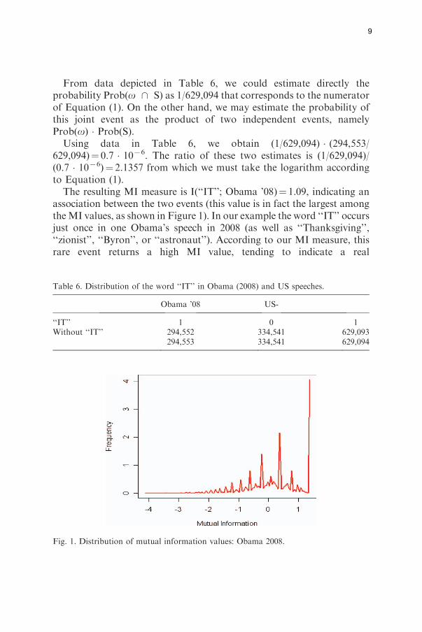
association between the two events (this value is in fact the largest amongtheMI values, as shown in Figure 1). In our example the word ‘‘IT’’ occursjust once in one Obama’s speech in 2008 (as well as ‘‘Thanksgiving’’,‘‘zionist’’, ‘‘Byron’’, or ‘‘astronaut’’). According to our MI measure, thisrare event returns a high MI value, tending to indicate a real

Table 6. Distribution of the word ‘‘IT’’ in Obama (2008) and US speeches.

Obama ’08 US-

‘‘IT’’ 1 0 1Without ‘‘IT’’ 294,552 334,541 629,093

294,553 334,541 629,094

Fig. 1. Distribution of mutual information values: Obama 2008.

9

association between the word ‘‘IT’’ and Obama’s vocabulary. Only oneoccurrence of this term can be found however and to ignore suchparticular cases, it is suggested that the additional constraint of a� 5 beimposed.The chi-square (w2) measure (Manning & Schutze, 2000) provides a

second approach to measuring the association between a word and a set ofdocuments. This method allows us to compare the observed frequency(e.g., the value a) with the expected number of tokens, under theassumption that the two events (o and S) are independent. This lattervalue is estimated using as n Prob(o) � Prob(S)¼ n � (aþ b)/n � (aþ c)/n¼(aþ b) � (aþ c)/n. Rather than being limited to comparing the single cellstoring the value a, we repeat this for the other three cells, namely b, c, and d.Equation (2) below shows the general formula used to compute the

chi-square measure, where oij indicates the observed frequencies (e.g., a,b, etc.) and eij the expected frequency stored in cell ij.

w2 ¼Xi;j¼1;2

ðoij � eijÞ2

eijð2Þ

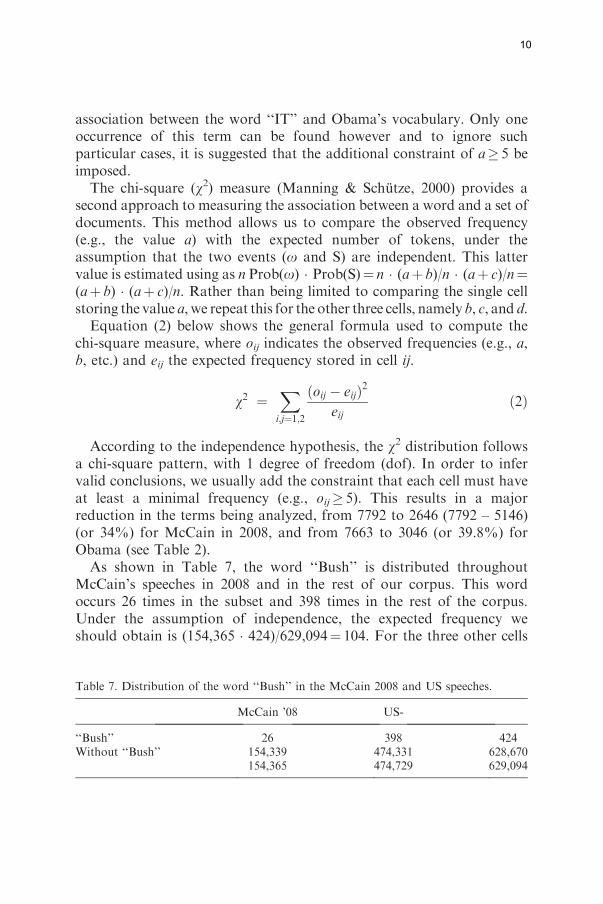
According to the independence hypothesis, the w2 distribution followsa chi-square pattern, with 1 degree of freedom (dof). In order to infervalid conclusions, we usually add the constraint that each cell must haveat least a minimal frequency (e.g., oij� 5). This results in a majorreduction in the terms being analyzed, from 7792 to 2646 (7792 – 5146)(or 34%) for McCain in 2008, and from 7663 to 3046 (or 39.8%) forObama (see Table 2).As shown in Table 7, the word ‘‘Bush’’ is distributed throughout

McCain’s speeches in 2008 and in the rest of our corpus. This wordoccurs 26 times in the subset and 398 times in the rest of the corpus.Under the assumption of independence, the expected frequency weshould obtain is (154,365 � 424)/629,094¼ 104. For the three other cells

Table 7. Distribution of the word ‘‘Bush’’ in the McCain 2008 and US speeches.

McCain ’08 US-

‘‘Bush’’ 26 398 424Without ‘‘Bush’’ 154,339 474,331 628,670

154,365 474,729 629,094

10

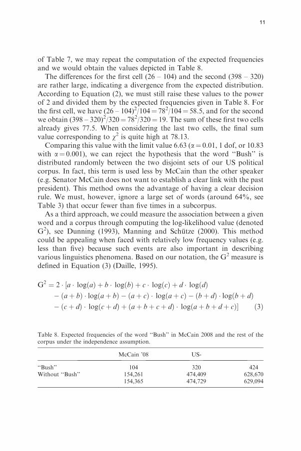
of Table 7, we may repeat the computation of the expected frequenciesand we would obtain the values depicted in Table 8.The differences for the first cell (26 – 104) and the second (398 – 320)

are rather large, indicating a divergence from the expected distribution.According to Equation (2), we must still raise these values to the powerof 2 and divided them by the expected frequencies given in Table 8. Forthe first cell, we have (26 – 104)2/104¼ 782/104¼ 58.5, and for the secondwe obtain (398 – 320)2/320¼ 782/320¼ 19. The sum of these first two cellsalready gives 77.5. When considering the last two cells, the final sumvalue corresponding to w2 is quite high at 78.13.Comparing this value with the limit value 6.63 (a¼ 0.01, 1 dof, or 10.83

with a¼ 0.001), we can reject the hypothesis that the word ‘‘Bush’’ isdistributed randomly between the two disjoint sets of our US politicalcorpus. In fact, this term is used less by McCain than the other speaker(e.g. Senator McCain does not want to establish a clear link with the pastpresident). This method owns the advantage of having a clear decisionrule. We must, however, ignore a large set of words (around 64%, seeTable 3) that occur fewer than five times in a subcorpus.As a third approach, we could measure the association between a given

word and a corpus through computing the log-likelihood value (denotedG2), see Dunning (1993), Manning and Schutze (2000). This methodcould be appealing when faced with relatively low frequency values (e.g.less than five) because such events are also important in describingvarious linguistics phenomena. Based on our notation, the G2 measure isdefined in Equation (3) (Daille, 1995).

G2 ¼ 2 � ½a � logðaÞ þ b � logðbÞ þ c � logðcÞ þ d � logðdÞ� ðaþ bÞ � logðaþ bÞ � ðaþ cÞ � logðaþ cÞ � ðbþ dÞ � logðbþ dÞ� ðcþ dÞ � logðcþ dÞ þ ðaþ bþ cþ dÞ � logðaþ bþ dþ cÞ� ð3Þ

Table 8. Expected frequencies of the word ‘‘Bush’’ in McCain 2008 and the rest of thecorpus under the independence assumption.

McCain ’08 US-

‘‘Bush’’ 104 320 424Without ‘‘Bush’’ 154,261 474,409 628,670

154,365 474,729 629,094

11

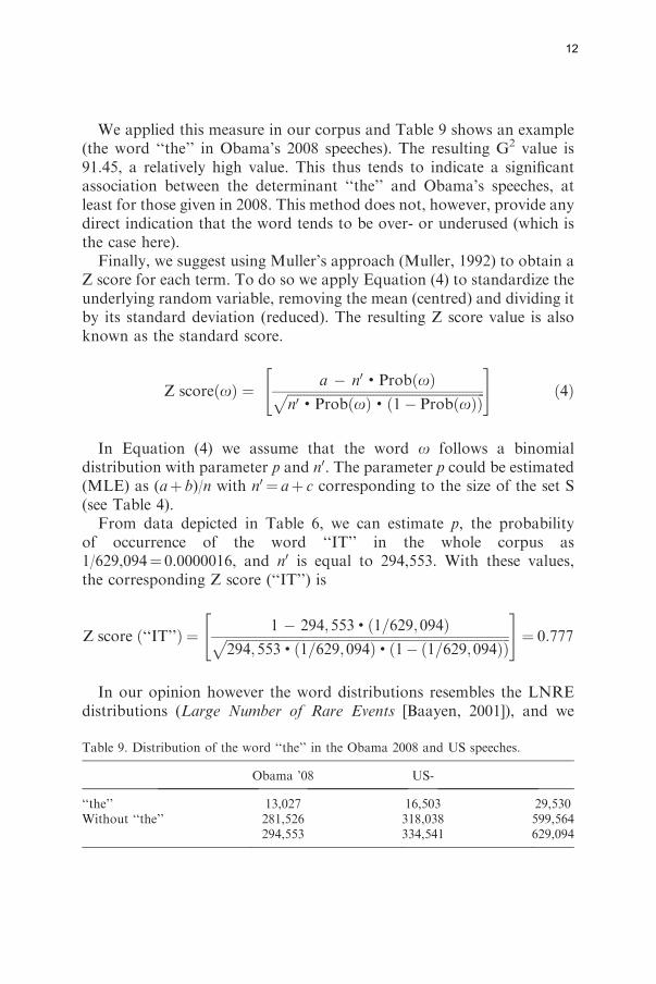
We applied this measure in our corpus and Table 9 shows an example(the word ‘‘the’’ in Obama’s 2008 speeches). The resulting G2 value is91.45, a relatively high value. This thus tends to indicate a significantassociation between the determinant ‘‘the’’ and Obama’s speeches, atleast for those given in 2008. This method does not, however, provide anydirect indication that the word tends to be over- or underused (which isthe case here).Finally, we suggest using Muller’s approach (Muller, 1992) to obtain a

Z score for each term. To do so we apply Equation (4) to standardize theunderlying random variable, removing the mean (centred) and dividing itby its standard deviation (reduced). The resulting Z score value is alsoknown as the standard score.

Z scoreðoÞ ¼ a � n0 � ProbðoÞffiffiffiffiffiffiffiffiffiffiffiffiffiffiffiffiffiffiffiffiffiffiffiffiffiffiffiffiffiffiffiffiffiffiffiffiffiffiffiffiffiffiffiffiffiffiffiffiffiffiffiffiffiffiffiffiffiffiffiffin0 � ProbðoÞ � ð1� ProbðoÞÞ

p" #

ð4Þ

In Equation (4) we assume that the word o follows a binomialdistribution with parameter p and n0. The parameter p could be estimated(MLE) as (aþ b)/n with n0 ¼ aþ c corresponding to the size of the set S(see Table 4).From data depicted in Table 6, we can estimate p, the probability

of occurrence of the word ‘‘IT’’ in the whole corpus as1/629,094¼ 0.0000016, and n0 is equal to 294,553. With these values,the corresponding Z score (‘‘IT’’) is

Z score ð‘‘IT’’Þ ¼ 1 � 294;553 � 1=629;094ð Þffiffiffiffiffiffiffiffiffiffiffiffiffiffiffiffiffiffiffiffiffiffiffiffiffiffiffiffiffiffiffiffiffiffiffiffiffiffiffiffiffiffiffiffiffiffiffiffiffiffiffiffiffiffiffiffiffiffiffiffiffiffiffiffiffiffiffiffiffiffiffiffiffiffiffiffiffiffiffiffiffiffiffiffiffiffi294;553 � 1=629;094ð Þ � 1� 1=629;094ð Þð Þ

p" #

¼ 0:777

In our opinion however the word distributions resembles the LNREdistributions (Large Number of Rare Events [Baayen, 2001]), and we

Table 9. Distribution of the word ‘‘the’’ in the Obama 2008 and US speeches.

Obama ’08 US-

‘‘the’’ 13,027 16,503 29,530Without ‘‘the’’ 281,526 318,038 599,564

294,553 334,541 629,094

12

would therefore suggest smoothing the estimation of the underlyingprobability p as (aþ bþ l)/(nþ l � jV j), where l is a smoothingparameter (set to 0.5 in our case) and jV j indicates vocabulary size (or12,573 in the current case). This modification will slightly shift theprobability density function’s mass towards rare and unseen words (orwords that do not yet occur) (Manning & Schutze, 2000).In our previous example, the new estimate for p is (1þ 0.5)/

(629,094þ 0.5 � 12,573)¼ 0.0000024, a value slightly larger than theprevious one. The resulting Z score is also slightly different (0.365).As a rule governing our decision we would consider those terms having

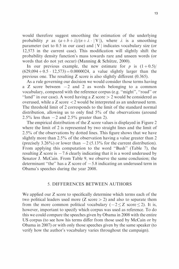
a Z score between 72 and 2 as words belonging to a commonvocabulary, compared with the reference corpus (e.g. ‘‘might’’, ‘‘road’’ or‘‘land’’ in our case). A word having a Z score4 2 would be considered asoverused, while a Z score52 would be interpreted as an underused term.The threshold limit of 2 corresponds to the limit of the standard normaldistribution, allowing us to only find 5% of the observations (around2.5% less than 72 and 2.5% greater than 2).The empirical distribution of the Z score values is displayed in Figure 2

where the limit of 2 is represented by two straight lines and the limit of2.5% of the observations by dotted lines. This figure shows that we haveslightly more than 2.5% of the observation having a value greater than 2(precisely 3.26%) or lower than 72 (5.13% for the current distribution).From applying this computation to the word ‘‘Bush’’ (Table 7), theresulting Z score is 77.6 clearly indicating that it is a word underused bySenator J. McCain. From Table 9, we observe the same conclusion; thedeterminant ‘‘the’’ has a Z score of 75.8 indicating an underused term inObama’s speeches during the year 2008.

5. DIFFERENCES BETWEEN AUTHORS

We applied our Z score to specifically determine which terms each of thetwo political leaders used more (Z score4 2) and also to separate themfrom the more common political vocabulary (72�Z score� 2). It is,however, important to specify which corpus was used as reference. To dothis we could compare the speeches given by Obama in 2008 with the entireUS corpus (to see how his terms differ from those used by McCain or byObama in 2007) or with only those speeches given by the same speaker (toverify how the author’s vocabulary varies throughout the campaign).

13

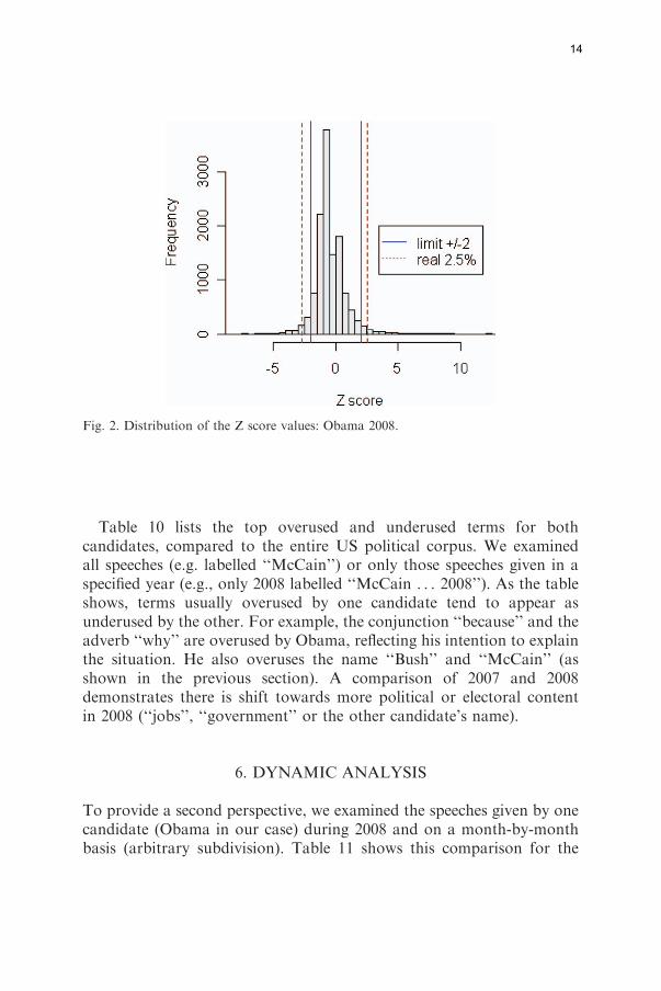
Table 10 lists the top overused and underused terms for bothcandidates, compared to the entire US political corpus. We examinedall speeches (e.g. labelled ‘‘McCain’’) or only those speeches given in aspecified year (e.g., only 2008 labelled ‘‘McCain . . . 2008’’). As the tableshows, terms usually overused by one candidate tend to appear asunderused by the other. For example, the conjunction ‘‘because’’ and theadverb ‘‘why’’ are overused by Obama, reflecting his intention to explainthe situation. He also overuses the name ‘‘Bush’’ and ‘‘McCain’’ (asshown in the previous section). A comparison of 2007 and 2008demonstrates there is shift towards more political or electoral contentin 2008 (‘‘jobs’’, ‘‘government’’ or the other candidate’s name).

6. DYNAMIC ANALYSIS

To provide a second perspective, we examined the speeches given by onecandidate (Obama in our case) during 2008 and on a month-by-monthbasis (arbitrary subdivision). Table 11 shows this comparison for the

Fig. 2. Distribution of the Z score values: Obama 2008.

14

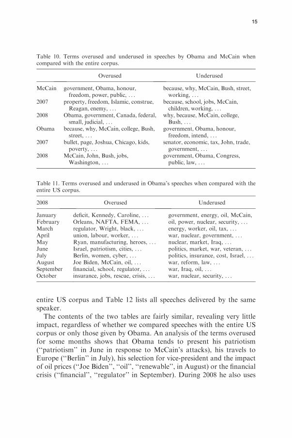
entire US corpus and Table 12 lists all speeches delivered by the samespeaker.The contents of the two tables are fairly similar, revealing very little

impact, regardless of whether we compared speeches with the entire UScorpus or only those given by Obama. An analysis of the terms overusedfor some months shows that Obama tends to present his patriotism(‘‘patriotism’’ in June in response to McCain’s attacks), his travels toEurope (‘‘Berlin’’ in July), his selection for vice-president and the impactof oil prices (‘‘Joe Biden’’, ‘‘oil’’, ‘‘renewable’’, in August) or the financialcrisis (‘‘financial’’, ‘‘regulator’’ in September). During 2008 he also uses

Table 10. Terms overused and underused in speeches by Obama and McCain whencompared with the entire corpus.

Overused Underused

McCain government, Obama, honour,freedom, power, public, . . .

because, why, McCain, Bush, street,working, . . .

2007 property, freedom, Islamic, construe,Reagan, enemy, . . .

because, school, jobs, McCain,children, working, . . .

2008 Obama, government, Canada, federal,small, judicial, . . .

why, because, McCain, college,Bush, . . .

Obama because, why, McCain, college, Bush,street, . . .

government, Obama, honour,freedom, intend, . . .

2007 bullet, page, Joshua, Chicago, kids,poverty, . . .

senator, economic, tax, John, trade,government, . . .

2008 McCain, John, Bush, jobs,Washington, . . .

government, Obama, Congress,public, law, . . .

Table 11. Terms overused and underused in Obama’s speeches when compared with theentire US corpus.

2008 Overused Underused

January deficit, Kennedy, Caroline, . . . government, energy, oil, McCain,February Orleans, NAFTA, FEMA, . . . oil, power, nuclear, security, . . .March regulator, Wright, black, . . . energy, worker, oil, tax, . . .April union, labour, worker, . . . war, nuclear, government, . . .May Ryan, manufacturing, heroes, . . . nuclear, market, Iraq, . . .June Israel, patriotism, cities, . . . politics, market, war, veteran, . . .July Berlin, women, cyber, . . . politics, insurance, cost, Israel, . . .August Joe Biden, McCain, oil, . . . war, reform, law, . . .September financial, school, regulator, . . . war, Iraq, oil, . . .October insurance, jobs, rescue, crisis, . . . war, nuclear, security, . . .

15

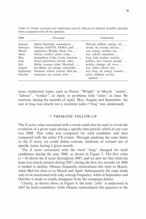
more traditional topics such as Pastor ‘‘Wright’’ in March, ‘‘union’’,‘‘labour’’, ‘‘worker’’, in April, or problems with ‘‘cities’’ in June. Bycontrast, during the months of April, May, August and September, thewar in Iraq was clearly not a recurrent topic (‘‘Iraq’’ was underused).

7. THEMATIC FOLLOW-UP

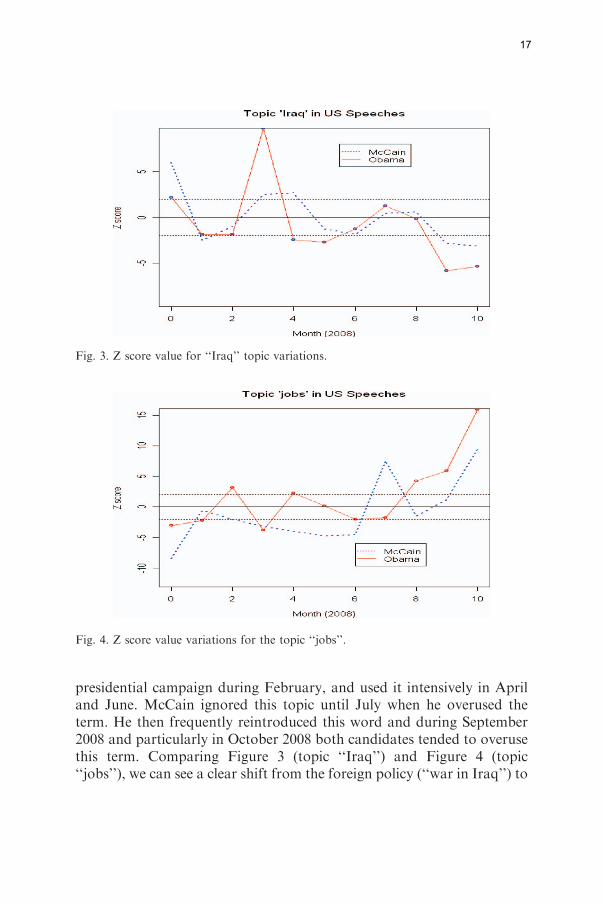
The Z score value associated with a word could also be used to reveal theevolution of a given topic during a specific time period, which in our casewas 2008. This value was computed for each candidate and thencompared with the entire US corpus. Through applying the same limitsto the Z score, we could define overuse, underuse or normal use ofspecific terms during a given month.The Z score associated with the word ‘‘Iraq’’ changed for both

candidates during the year 2008, as shown in Figure 3. The first value(x¼ 0) shows the Z score throughout 2007, and we also see that while hisissue was clearly present during 2007, during the first two months on 2008it tended to decline. Obama frequently reintroduces this term in March,while McCain does so in March and April. Subsequently the topic tendsonly to be mentioned with only average frequency, while in September andOctober it tends to totally disappear from the campaign debate.Clearly, as shown above in Figure 4, the term ‘‘jobs’’ is underused in

2007 by both candidates, while Obama reintroduced this question in the

Table 12. Terms overused and underused used by Obama in selected monthly speecheswhen compared with all his speeches.

2008 Overused Underused

January deficit, Kennedy, assumption, . . . McCain, million, energy, oil, . . .February Orleans, NAFTA, FEMA, gulf, . . . world, oil, women, history, . . .March regulatory, Wright, black, war, . . . you, energy, worker, tax, . . .April labour, worker, union, trade, . . . war, school, education, . . .May hemisphere, Cuba, Latin, freedom, . . . Iraq, kids, nuclear, market, . . .June Israel, patriotism, Jewish, cities, . . . politics, war, veteran, people, . . .July Berlin, women, cyber, Marshall, . . . politics, change, tell, story, . . .August Joe Biden, oil, energy, renewable, . . . war, white, school, law, . . .September financial, school, courses, McCain, . . . war, Iraq, oil, energy, women, . . .October insurance, tax, rescue, jobs, . . . party, children, service,

nuclear, . . .

16

presidential campaign during February, and used it intensively in Apriland June. McCain ignored this topic until July when he overused theterm. He then frequently reintroduced this word and during September2008 and particularly in October 2008 both candidates tended to overusethis term. Comparing Figure 3 (topic ‘‘Iraq’’) and Figure 4 (topic‘‘jobs’’), we can see a clear shift from the foreign policy (‘‘war in Iraq’’) to

Fig. 3. Z score value for ‘‘Iraq’’ topic variations.

Fig. 4. Z score value variations for the topic ‘‘jobs’’.

17

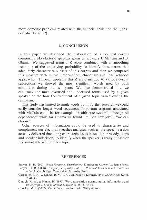
more domestic problems related with the financial crisis and the ‘‘jobs’’(see also Table 12).

8. CONCLUSION

In this paper we described the elaboration of a political corpuscomprising 245 electoral speeches given by senators J. McCain and B.Obama. We suggested using a Z score combined with a smoothingtechnique of the underlying probability to identify those terms thatadequately characterize subsets of this corpus and then we comparedthis measure with mutual information, chi-square and log-likelihoodapproaches. Through applying this Z score method to various corpussubsections we showed the most significant words used by bothcandidates during the two years. We also demonstrated how wecan track the most overused and underused terms used by a givenspeaker or the how the treatment of a given topic varied during thecampaign.This study was limited to single words but in further research we could

easily consider longer word sequences. Important trigrams associatedwith McCain could be for example: ‘‘health care system’’, ‘‘foreign oildependence’’ while for Obama we found ‘‘million new jobs’’, ‘‘we canchoose’’.Other sources of information could be used to characterize and

complement our electoral speeches analyses, such as the speech versionactually delivered (including characteristics as intonation, prosody, stopsand speaker indecision) to identify when the speaker is really at ease oruncomfortable with a given topic.

REFERENCES

Baayen, H. R. (2001). Word Frequency Distributions. Dordrecht: Kluwer Academic Press.Baayen, H. R. (2008). Analyzing Linguistic Data: A Practical Introduction to Statistics

using R. Cambridge: Cambridge University Press.Carpenter, R. H., & Seltzer, R. V. (1970). On Nixon’s Kennedy style. Speaker and Gavel,

7, 41–43.Church, K. W., & Hanks, P. (1990). Word association norms, mutual information, and

lexicography. Computational Linguistics, 16(1), 22–29.Crawley, M. J. (2007). The R Book. London: John Wiley & Sons.

18

Daille, B. (1995). Combined approach for terminology extraction: Lexical statistics andlinguistic filtering. UCREL Technical Papers. Vol 5. University of Lancaster.

Dunning, T. (1993). Accurate methods for the statistics of surprise and coincidence.Computational Linguistics, 19(1), 61–74.

Herman, V. (1974). What governments say and what governments do: An analysis ofpost-war Queen’s speeches. Parliamentary Affairs, 28(1), 22–31.

Kilgarriff, A. (2001). Comparing corpora. International Journal of Corpus Linguistics,6(1), 97–133.

Francis, W. N., & Kucera, H. (1982). Frequency Analysis of English Usage: Lexicon andGrammar. Boston: Houghton Mifflin.

Labbe, D. (2007). Experiments on authorship attribution by intertextual distance inEnglish. Journal of Quantitative Linguistics, 14(1), 33–80.

Labbe, D., & Moniere, D. (2003). Le discours gouvernemental. Canada, Quebec, France(1945–2000). Paris: Honore Champion.

Labbe, D., & Moniere, D. (2008). Les mots qui nous gouvernent. Le discours des premiersministres quebecois: 1960–2005. Montreal: Moniere-Wollank.

Manning, C. D., & Schutze, H. (2000). Foundations of Statistical Natural LanguageProcessing. Cambridge: The MIT Press.

Muller, C. (1992). Principes et methodes de statistique lexicale. Paris: Honore Champion.Nugues, P. M. (2006). An Introduction to Language Processing with Perl and Prolog.

Berlin: Springer-Verlag.Toutanova, K., & Manning, C. (2000). Enriching the knowledge sources used in a

maximum entropy part-of-speech tagging. In Proceedings of the Joint SIGDATConference on Empirical Methods in Natural Language Processing and Very LargeCorpora (EMNLP/VLC-2000), 63–70.

Toutanova, K., Klein, D., Manning, C., & Singer, Y. (2003). Feature-rich part-of-speechtagging with a cyclid dependency network. Proceedings of HLT-NAACL 2003,252–259.

19