


Languages
Pages
Legal


Chapter 8: Estimating volatility and correlations
Lecture Quantitative Finance
Spring 2011
Prof. Dr. Erich Walter Farkas
Lecture 12: May 19, 2011Chapter 8: Estimating volatility and correlations
Prof. Dr. Erich Walter Farkas Quantitative Finance 11: Lecture 12 1 / 49

Chapter 8: Estimating volatility and correlations
IntroductionEstimating volatility: EWMA and GARCH (1,1)Maximum Likelihood methodsCorrelations
1 Chapter 8: Estimating volatility and correlationsIntroductionEstimating volatility: EWMA and GARCH (1,1)Maximum Likelihood methodsCorrelations
Prof. Dr. Erich Walter Farkas Quantitative Finance 11: Lecture 12 2 / 49
Chapter 8: Estimating volatility and correlations
IntroductionEstimating volatility: EWMA and GARCH (1,1)Maximum Likelihood methodsCorrelations
Outline
1 Introduction
2 Estimating volatility
3 The exponentially weighted moving average model
4 The GARCH (1,1) model
5 Maximum Likelihood methods
6 Using GARCH (1,1) to forecast future volatility
7 Correlations
Prof. Dr. Erich Walter Farkas Quantitative Finance 11: Lecture 12 3 / 49

Chapter 8: Estimating volatility and correlations
IntroductionEstimating volatility: EWMA and GARCH (1,1)Maximum Likelihood methodsCorrelations
Introduction
the goal of this chapter is to explain how historical data can be used to produceestimates of the current and future levels of volatilities and correlations
this problem is relevant both to the calculation of value at risk and to thevaluation of derivatives
we consider the following models
1 exponentially weighted moving average (EWMA)2 autoregressive conditional heteroscedascity (ARCH)3 generalized A R C H (GARCH)
the distinctive feature is that they recognize that volatilities and correlations arenot constant
during some periods, a particular volatility or correlation may be relatively low,whereas during other periods it may be relatively high
the models attempt to keep track of the variations in the volatility or correlationthrough time
Prof. Dr. Erich Walter Farkas Quantitative Finance 11: Lecture 12 4 / 49

Chapter 8: Estimating volatility and correlations
IntroductionEstimating volatility: EWMA and GARCH (1,1)Maximum Likelihood methodsCorrelations
Introduction
to estimate the volatility of a stock empirically, the stock price is usuallyobserved at fixed intervals of time (e.g. every day, week, or month)
consider
n + 1 : number of observations
Si : stock price at end of the i th interval, with i = 0, 1, ...n
τ : length of time intervals in years
and let
ui = log
(Si
Si−1
)i = 1, 2, ..., n
the usual estimate s of the standard deviation of the ui is given by
s =
√√√√ 1
n − 1
n∑i=1
(ui − u)2
where u is the mean of uiσ can be estimated as σ = s√
τ
the standard error or this estimate can be shown to be approximatively σ/(√
2n)
Prof. Dr. Erich Walter Farkas Quantitative Finance 11: Lecture 12 5 / 49

Chapter 8: Estimating volatility and correlations
IntroductionEstimating volatility: EWMA and GARCH (1,1)Maximum Likelihood methodsCorrelations
Introduction
note that the usual estimate s of the standard deviation of the ui is given also by
s =
√√√√ 1
n − 1
n∑i=1
u2i −
1
n(n − 1)
(n∑
i=1
ui
)2
where u is the mean of ui
Prof. Dr. Erich Walter Farkas Quantitative Finance 11: Lecture 12 6 / 49

Chapter 8: Estimating volatility and correlations
IntroductionEstimating volatility: EWMA and GARCH (1,1)Maximum Likelihood methodsCorrelations
Introduction
choosing an appropriate value for n is not easy
more data generally lead to more accuracy, but σ does change over time anddata that are too old may not be relevant for predicting the future volatility
a compromise that seems to work reasonably well is to use closing prices fromdaily data over the most recent 90 to 180 days
an often used rule of the thumb is to set n equal to the number of days towhich the volatility is to be applied
thus, if the volatility estimate is to be used to value a 2-year option, daily datafor the last 2 years are used
Prof. Dr. Erich Walter Farkas Quantitative Finance 11: Lecture 12 7 / 49

Chapter 8: Estimating volatility and correlations
IntroductionEstimating volatility: EWMA and GARCH (1,1)Maximum Likelihood methodsCorrelations
Introduction: Example
A sequence of stock prices during 21 consecutive trading days:
Day Closing stock price Si/Si−1 ui = log(Si/Si−1)
0 20.001 20.10 1.00500 0.004992 19.90 0.99005 0.010003 20.00 1.00503 0.005014 20.50 1.02500 0.024695 20.25 0.98780 −0.012276 20.90 1.03210 0.031597 20.90 1.00000 0.000008 20.90 1.00000 0.000009 20.75 0.99282 −0.00720
10 20.75 1.00000 0.0000011 21.00 1.01205 0.0119812 21.10 1.00476 0.0047513 20.90 0.99052 −0.0095214 20.90 1.00000 0.0000015 21.25 1.01675 0.0166116 21.40 1.00706 0.0070317 21.40 1.00000 0.0000018 21.25 0.99299 −0.0070319 21.75 1.02353 0.0232620 22.00 1.01149 0.01143
In this case ∑ui = 0.09531 and
∑u2i = 0.00326
Prof. Dr. Erich Walter Farkas Quantitative Finance 11: Lecture 12 8 / 49

Chapter 8: Estimating volatility and correlations
IntroductionEstimating volatility: EWMA and GARCH (1,1)Maximum Likelihood methodsCorrelations
Introduction: Example
the estimate of the standard deviation of the daily return is√0.00326
19−
0.095312
20 · 19= 0.01216 or 1.216%
assuming that there are 252 trading days per year, τ = 1/252 and the data givean estimate for the volatility per annum of
0.01216×√
252 = 0.193 or 19.3%
the standard error of this estimate is
0.193√
2× 20= 0.031 or 3.1% per annum
with dividend paying stocks: the return ui during a time interval that includesan ex-dividend day is given by
ui = logSi + D
Si−1
where D is the amount of the dividend
Prof. Dr. Erich Walter Farkas Quantitative Finance 11: Lecture 12 9 / 49

Chapter 8: Estimating volatility and correlations
IntroductionEstimating volatility: EWMA and GARCH (1,1)Maximum Likelihood methodsCorrelations
Introduction: Trading days vs. calendar days
an important issue is whether time should be measured in calendar days ortrading days when volatility parameters are being estimated and used
practitioners tend to ignore days when the exchange is closed when estimatingvolatility from historical data (and when calculating the life of an option)
the volatility per annum is calculated from the volatility per trading day usingthe formula
Vol per annum = Vol per tr. day×√
nr. of tr. days per annum
Prof. Dr. Erich Walter Farkas Quantitative Finance 11: Lecture 12 10 / 49

Chapter 8: Estimating volatility and correlations
IntroductionEstimating volatility: EWMA and GARCH (1,1)Maximum Likelihood methodsCorrelations
Introduction: What causes volatility?
it is natural to assume that the volatility of a stock is caused by newinformation reaching the market
this new information causes people to revise their opinions about the value ofthe stock: the price of the stock changes and volatility results
with several years of daily stock price date researchers can calculate:
1 the variance of the stock price returns between the close oftrading on one day and the close of trading on the next daywhen there are no intervening nontrading days (in fact avariance of returns over a 1-day period)
2 the variance of the stock price returns between the close oftrading on Friday and the close of trading on Monday (in facta variance of returns over 3-day period)
Prof. Dr. Erich Walter Farkas Quantitative Finance 11: Lecture 12 11 / 49

Chapter 8: Estimating volatility and correlations
IntroductionEstimating volatility: EWMA and GARCH (1,1)Maximum Likelihood methodsCorrelations
Introduction: What causes volatility?
we might be tempted to expect the second variance to be three times as greatas the first variancebut this is not the case (Fama 1965, French 1980, French and Roll 1980: secondvariance is respectively 22%, 19% and 10.7% higher than the first variance)
it seems that volatility is to a large extent caused by trading itself (tradersusually have no difficulty accepting this conclusion!)
Prof. Dr. Erich Walter Farkas Quantitative Finance 11: Lecture 12 12 / 49
Chapter 8: Estimating volatility and correlations
IntroductionEstimating volatility: EWMA and GARCH (1,1)Maximum Likelihood methodsCorrelations
Estimating volatility
define σn the volatility of a market variable on day n, as estimated at the end ofday n − 1
the square of the volatility σ2n on day n is the variance rate
the value of the market variable at the end of day i is Si
recall the variable ui is defined as the continuously compounded return duringday i (between the end of day i − 1 and the end of day i):
ui = logSi
Si−1
an unbiased estimate of the variance rate per day, σ2n, using the most recent m
observations on the ui is
σ2n =
1
m − 1
m∑i=1
(un−i − u)2
Prof. Dr. Erich Walter Farkas Quantitative Finance 11: Lecture 12 13 / 49

Chapter 8: Estimating volatility and correlations
IntroductionEstimating volatility: EWMA and GARCH (1,1)Maximum Likelihood methodsCorrelations
Estimating volatility
the mean u is given by
u =1
m
m∑i=1
un−i
recall an unbiased estimate of the variance rate per day, σ2n, using the most
recent m observations on the ui is
σ2n =
1
m − 1
m∑i=1
(un−i − u)2
for the purposes of monitoring daily volatility the last formula is usually changedin a number of ways:
Prof. Dr. Erich Walter Farkas Quantitative Finance 11: Lecture 12 14 / 49

Chapter 8: Estimating volatility and correlations
IntroductionEstimating volatility: EWMA and GARCH (1,1)Maximum Likelihood methodsCorrelations
Estimating volatility
1 ui is defined as the percentage change in the market variablebetween the end of day i − 1 and the end of day i , so that
ui =Si − Si−1
Si−1
2 u is assumed to be zero3 m − 1 is replaced by m
these three changes make very little difference to the estimates that arecalculated but they allow us to simplify the formula for the variance rate to
σ2n =
1
m
m∑i=1
u2n−i
last equation gives equal weight to u2n−1, u
2n−2, ..., u
2n−m
our objective is to estimate the current level of volatility σn: it therefore makessense to give more weight to recent data
Prof. Dr. Erich Walter Farkas Quantitative Finance 11: Lecture 12 15 / 49

Chapter 8: Estimating volatility and correlations
IntroductionEstimating volatility: EWMA and GARCH (1,1)Maximum Likelihood methodsCorrelations
Estimating volatility
a model that does it is:
σ2n =
m∑i=1
αiu2n−i (∗)
the variable αi is the amount of weight given to the observation i days ago
the numbers αi are positive
if we choose them so that αi < αj when i > j , less weight is given to olderobservations
the weights must sum up to unity, so we have
m∑i=1
αi = 1
Prof. Dr. Erich Walter Farkas Quantitative Finance 11: Lecture 12 16 / 49

Chapter 8: Estimating volatility and correlations
IntroductionEstimating volatility: EWMA and GARCH (1,1)Maximum Likelihood methodsCorrelations
Estimating volatility
an extension of the idea in equation (*) is to assume that there is a long-runaverage variance rate and that this should be given some weight
this leads to the model that take the form
σ2n = γVL +
m∑i=1
αiu2n−i (∗∗)
where VL is the long-run variance rate and γ is the weight assigned to VL
because the weights must sum to unity, we have
γ +m∑i=1
αi = 1
Prof. Dr. Erich Walter Farkas Quantitative Finance 11: Lecture 12 17 / 49
Chapter 8: Estimating volatility and correlations
IntroductionEstimating volatility: EWMA and GARCH (1,1)Maximum Likelihood methodsCorrelations
Estimating volatility
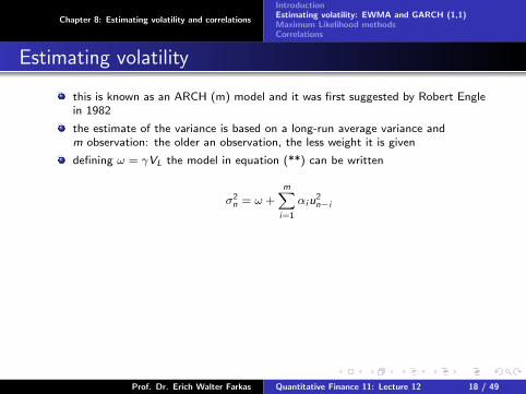
this is known as an ARCH (m) model and it was first suggested by Robert Englein 1982
the estimate of the variance is based on a long-run average variance andm observation: the older an observation, the less weight it is given
defining ω = γVL the model in equation (**) can be written
σ2n = ω +
m∑i=1
αiu2n−i
Prof. Dr. Erich Walter Farkas Quantitative Finance 11: Lecture 12 18 / 49

Chapter 8: Estimating volatility and correlations
IntroductionEstimating volatility: EWMA and GARCH (1,1)Maximum Likelihood methodsCorrelations
The EWMA model
the exponentially weighted moving average (EWMA) model is a particular caseof the model in equation (*) where the weights αi decrease exponentially as wemove back through time
specifically αi+1 = λαi where λ is a constant between 0 and 1
it turns out that this weighting scheme leads to a particularly simple formula forupdating volatility estimates:
σ2n = λσ2
n−1 + (1− λ)u2n−1 (1)
the estimate σn is the volatility for day n (made of the end of day n − 1) iscalculated from σn−1 (the estimate that was made at the end of day n − 2 ofthe volatility for day n − 1) and un−1 (the most recent percentage change)
Prof. Dr. Erich Walter Farkas Quantitative Finance 11: Lecture 12 19 / 49
Chapter 8: Estimating volatility and correlations
IntroductionEstimating volatility: EWMA and GARCH (1,1)Maximum Likelihood methodsCorrelations
The EWMA model
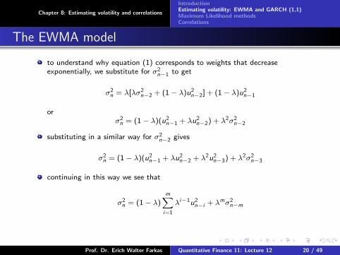
to understand why equation (1) corresponds to weights that decreaseexponentially, we substitute for σ2
n−1 to get
σ2n = λ[λσ2
n−2 + (1− λ)u2n−2] + (1− λ)u2
n−1
orσ2n = (1− λ)(u2
n−1 + λu2n−2) + λ2σ2
n−2
substituting in a similar way for σ2n−2 gives
σ2n = (1− λ)(u2
n−1 + λu2n−2 + λ2u2
n−3) + λ2σ2n−3
continuing in this way we see that
σ2n = (1− λ)
m∑i=1
λi−1u2n−i + λmσ2
n−m
Prof. Dr. Erich Walter Farkas Quantitative Finance 11: Lecture 12 20 / 49

Chapter 8: Estimating volatility and correlations
IntroductionEstimating volatility: EWMA and GARCH (1,1)Maximum Likelihood methodsCorrelations
The EWMA model
recall
σ2n = (1− λ)
m∑i=1
λi−1u2n−i + λmσ2
n−m
for large m the term λmσ2n−m is sufficiently small to be ignored so that
equation (1) is the same as equation (*) with αi = (1− λ)λi−1
the weights for the ui decline at rate λ as we move back thorugh time; eachweight is λ times the previous weight
Prof. Dr. Erich Walter Farkas Quantitative Finance 11: Lecture 12 21 / 49

Chapter 8: Estimating volatility and correlations
IntroductionEstimating volatility: EWMA and GARCH (1,1)Maximum Likelihood methodsCorrelations
The EWMA model: Example
suppose that λ = 0.90, the volatility estimated for a market variable forday n − 1 is 1% per day and during day n − 1 the market variable increasedby 2%
this means σ2n−1 = 0.012 = 0.0001 and u2
n−1 = 0.022 = 0.0004
equation (1) gives
σ2n = 0.9× 0.0001 + 0.1× 0.0004 = 0.00013
the estimate of the volatility σn for day n is therefore√
0.00013 or 1.14% perday
note that the expected value of u2n−1 is σ2
n−1 or 0.0001
in this example, the realized value of u2n−1 is greater than the expected value
and as a result our volatility estimate increases
if the realized value of u2n−1 had been less than its expected value, our estimate
of the volatility would have decreased
Prof. Dr. Erich Walter Farkas Quantitative Finance 11: Lecture 12 22 / 49

Chapter 8: Estimating volatility and correlations
IntroductionEstimating volatility: EWMA and GARCH (1,1)Maximum Likelihood methodsCorrelations
The EWMA model
the EWMA approach has the attractive feature that relatively little data need tobe stored
at any given time we need to remember only the current estimate of the variancerate and the most recent observation on the value of the market variable
when we get a new observation on the value of the market variable, we calculatea new daily percentage change and use equation (1) to update our estimate ofthe variance rate
the old estimate of the variance rate and the old value of the market variablecan then be discarded
the EWMA approach is designed to track changes in the volatility
the Risk Metrics database, which was originally created by J. P. Morgan andmade publicly available in 1994, uses the EWMA model with λ = 0.94 forupdating daily volatility estimates in its RiskMetrics database
the company found that, across a range of different market variables, this valueof λ gives forecasts of the variance rate that come closest to the realizedvariance rate
Prof. Dr. Erich Walter Farkas Quantitative Finance 11: Lecture 12 23 / 49

Chapter 8: Estimating volatility and correlations
IntroductionEstimating volatility: EWMA and GARCH (1,1)Maximum Likelihood methodsCorrelations
The GARCH (1,1) model
proposed by T. Bollerslev in 1986
the difference between GARCH (1,1) and EWMA is analogous to the differencebetween equation (*) and equation (**)
in GARCH (1,1) σ2n is calculated from the long-run average variance rate VL as
well as from σn−1 and un−1
the equation for GARCH (1,1) is
σ2n = γVL + αu2
n−1 + βσ2n−1
where γ is the weight assigned to VL, α is the weight assigned to u2n−1 and β is
the weight assigned to σ2n−1
the weights sum up to oneγ + α+ β = 1
Prof. Dr. Erich Walter Farkas Quantitative Finance 11: Lecture 12 24 / 49

Chapter 8: Estimating volatility and correlations
IntroductionEstimating volatility: EWMA and GARCH (1,1)Maximum Likelihood methodsCorrelations
The GARCH (1,1) model
the EWMA model is a particular case of GARCH (1,1) where γ = 0, α = 1− λ,β = λ
the (1,1) in GARCH (1,1) indicates that σ2n is based on the most recent
observation of u2 and the most recent estimate of the variance rate
the more general GARCH (p,q) model calculates σ2n from the most recent p
observations on u2 and the most q estimates of the variance rate; GARCH (1,1)is by far the most popular of the GARCH models
setting ω = γVL, the GARCH (1,1) model can also be written
σ2n = ω + αu2
n−1 + βσ2n−1
the last form is usually used for the purposes of estimating the parameters
for a stable GARCH (1,1) process we require α+ β < 1, otherwise the weightterm applied to the long-term variance is negative
Prof. Dr. Erich Walter Farkas Quantitative Finance 11: Lecture 12 25 / 49

Chapter 8: Estimating volatility and correlations
IntroductionEstimating volatility: EWMA and GARCH (1,1)Maximum Likelihood methodsCorrelations
The GARCH (1,1) model: Example
suppose that a GARCH (1,1) model is estimated from daily data as
σ2n = 0.000002 + 0.13u2
n−1 + 0.86σ2n−1
this corresponds to α = 0.13, β = 0.86 and ω = 0.000002
because γ = 1− α− β it follows that γ = 0.01
because ω = γVL it follows that VL = 0.0002
in other words, the long-run average variance per day implied by the modelis 0.0002
this corresponds to a volatility of√
0.0002 = 0.014 or 1.4% per day
suppose that the estimate of the volatility on day n − 1 is 1.6% per day, so thatσ2n−1 = 0.0162 = 0.000256 and that on day n − 1 the market variable decreased
by 1% so that u2n−1 = 0.012 = 0.0001
then
σ2n = 0.000002 + 0.13× 0.0001 + 0.86× 0.000256 = 0.00023516
the new estimate of the volatility is therefore√
0.00023516 = 0.0153 or 1.53%
Prof. Dr. Erich Walter Farkas Quantitative Finance 11: Lecture 12 26 / 49

Chapter 8: Estimating volatility and correlations
IntroductionEstimating volatility: EWMA and GARCH (1,1)Maximum Likelihood methodsCorrelations
The GARCH (1,1) model: The weights
as in the EWMA model we immediately get
σ2n = ω + βω + β2ω + αu2
n−1 + αβu2n−2 + αβ2u2
n−3 + β3σ2n−3
continuing in this was we see that the weight applied to u2n−i is αβi−1
the weights decline exponentially at rate β
the parameter β can be interpreted as decay rate; it is similar to the λ in theEWMA model
the GARCH (1,1) model is similar to the EWMA model except that, in additionto assigning weights that decline exponentially to past u2 it also assigns someweight to the long-run average volatility
Prof. Dr. Erich Walter Farkas Quantitative Finance 11: Lecture 12 27 / 49
Chapter 8: Estimating volatility and correlations
IntroductionEstimating volatility: EWMA and GARCH (1,1)Maximum Likelihood methodsCorrelations
The GARCH (1,1) model: Mean reversion (optional part)
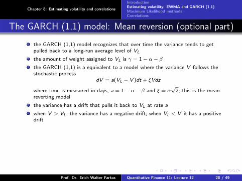
the GARCH (1,1) model recognizes that over time the variance tends to getpulled back to a long-run average level of VL
the amount of weight assigned to VL is γ = 1− α− βthe GARCH (1,1) is a equivalent to a model where the variance V follows thestochastic process
dV = a(VL − V )dt + ξVdz
where time is measured in days, a = 1− α− β and ξ = α√
2; this is the meanreverting model
the variance has a drift that pulls it back to VL at rate a
when V > VL, the variance has a negative drift; when VL < V it has a positivedrift
Prof. Dr. Erich Walter Farkas Quantitative Finance 11: Lecture 12 28 / 49

Chapter 8: Estimating volatility and correlations
IntroductionEstimating volatility: EWMA and GARCH (1,1)Maximum Likelihood methodsCorrelations
Choosing between the models
in practice variance rates tend to be mean reverting
the GARCH (1,1) model incorporates mean reversion, whereas the EWMAmodel does not
GARCH (1,1) is therefore more appealing than the EWMA model
a question that needs to be discussed is how best-fit parameters ω, α, β inGARCH (1,1) can be estimated
when the parameter ω is zero, the GARCH (1,1) reduces to EWMA
in circumstances where the best-fit value of ω turns out to be negative, theGARCH (1,1) model is not stable and it makes sense to switch to the EWMAmodel
Prof. Dr. Erich Walter Farkas Quantitative Finance 11: Lecture 12 29 / 49
Chapter 8: Estimating volatility and correlations
IntroductionEstimating volatility: EWMA and GARCH (1,1)Maximum Likelihood methodsCorrelations
Maximum Likelihood methods
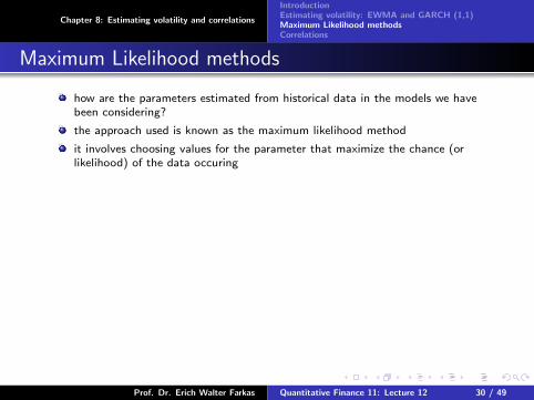
how are the parameters estimated from historical data in the models we havebeen considering?
the approach used is known as the maximum likelihood method
it involves choosing values for the parameter that maximize the chance (orlikelihood) of the data occuring
Prof. Dr. Erich Walter Farkas Quantitative Finance 11: Lecture 12 30 / 49

Chapter 8: Estimating volatility and correlations
IntroductionEstimating volatility: EWMA and GARCH (1,1)Maximum Likelihood methodsCorrelations
Estimating a constant variance
problem: estimate the variance of a variable X from m observations on X whenthe underlying distribution is normal with zero mean
we assume that the observations are u1, u2, ... and that the mean of theunderlying distribution is zero
denote the variance with v
the likelihood of ui being observed is the probability density function for Xwhen X = ui
this is
1√
2πvexp
(−u2
i
2v
)the likelihood of m observations occuring in order in which they are observed is
m∏i=1
[1
√2πv
exp
(−u2
i
2v
)]
using the maximum likelihood method, the best estimate of v is the value thatmaximizes this expression
Prof. Dr. Erich Walter Farkas Quantitative Finance 11: Lecture 12 31 / 49

Chapter 8: Estimating volatility and correlations
IntroductionEstimating volatility: EWMA and GARCH (1,1)Maximum Likelihood methodsCorrelations
Estimating a constant variance
maximizing an expression is equivalent to maximizing the logarithm of theexpression; taking logarithms and ignoring constant multiplicative factors, it canbe seen that we wish to maximize
m∑i=1
[− log v −
u2i
v
]
differentiating this expression with respect to v and setting the result equationto zero, we see that the maximum likelihood estimator of v is
1
m
m∑i=1
u2i
Prof. Dr. Erich Walter Farkas Quantitative Finance 11: Lecture 12 32 / 49

Chapter 8: Estimating volatility and correlations
IntroductionEstimating volatility: EWMA and GARCH (1,1)Maximum Likelihood methodsCorrelations
Estimating GARCH (1,1) parameters
how can the likelihood method be used to estimate the parameters whenGARCH (1,1) method or some other volatility update scheme is used?
define vi = σ2i as the variance estimated for day i
we assume that the probability distribution of ui conditional on the variance isnormal
a similar analysis to the one just given shows the best parameters are the onesthat maximize
m∏i=1
[1
√2πvi
exp
(−u2
i
2vi
)]
this is equivalent (taking logarithms) to maximizing
m∑i=1
[− log vi −
u2i
vi
](2)
this is the same expression as above, except that v is replaced by vi
we search iteratively to find the parameters in the model that maximize theexpression in (2)
Prof. Dr. Erich Walter Farkas Quantitative Finance 11: Lecture 12 33 / 49

Chapter 8: Estimating volatility and correlations
IntroductionEstimating volatility: EWMA and GARCH (1,1)Maximum Likelihood methodsCorrelations
Estimation of GARCH (1,1) parameters: Example
the data below analyses the Japanese yen exchange rate between January 6,1988 and August 15, 1997
Date Day i Si ui vi = σ2i − log(vi )− u2
i /vi
06− Jan − 88 1 0.00772807− Jan − 88 2 0.007779 0.00659908− Jan − 88 3 0.007746 −0.004242 0.00004355 9.628311− Jan − 88 4 0.007816 0.009037 0.00004198 8.132912− Jan − 88 5 0.007837 0.002687 0.00004455 9.856813− Jan − 88 6 0.007924 0.011101 0.00004220 7.1529
... ... ... ... ... ...13− Aug − 97 2421 0.008643 0.003374 0.00007626 9.332114− Aug − 97 2422 0.008493 −0.017309 0.00007092 5.329415− Aug − 97 2423 0.008495 0.000144 0.00008417 9.3824∑
= 22063.5763
Prof. Dr. Erich Walter Farkas Quantitative Finance 11: Lecture 12 34 / 49
Chapter 8: Estimating volatility and correlations
IntroductionEstimating volatility: EWMA and GARCH (1,1)Maximum Likelihood methodsCorrelations
Estimation of GARCH (1,1) parameters: Example
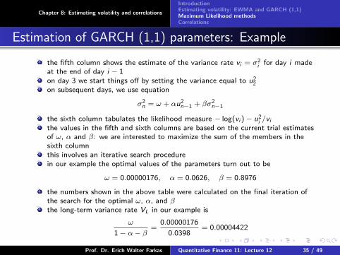
the fifth column shows the estimate of the variance rate vi = σ2i for day i made
at the end of day i − 1on day 3 we start things off by setting the variance equal to u2
2on subsequent days, we use equation
σ2n = ω + αu2
n−1 + βσ2n−1
the sixth column tabulates the likelihood measure − log(vi )− u2i /vi
the values in the fifth and sixth columns are based on the current trial estimatesof ω, α and β: we are interested to maximize the sum of the members in thesixth columnthis involves an iterative search procedurein our example the optimal values of the parameters turn out to be
ω = 0.00000176, α = 0.0626, β = 0.8976
the numbers shown in the above table were calculated on the final iteration ofthe search for the optimal ω, α, and βthe long-term variance rate VL in our example is
ω
1− α− β=
0.00000176
0.0398= 0.00004422
Prof. Dr. Erich Walter Farkas Quantitative Finance 11: Lecture 12 35 / 49

Chapter 8: Estimating volatility and correlations
IntroductionEstimating volatility: EWMA and GARCH (1,1)Maximum Likelihood methodsCorrelations
Estimation of GARCH (1,1) parameters: Example
when the EWMA model is used, the estimation procedure is relatively simple:we set ω = 0, α = 1− λ, and β = λ
in the table above, the value of λ that maximizes the objective functionis 0.9686 and the value of the objective function is 21995.8377
both GARCH (1,1) and the EWMA method can be implemented by using theSolver routine in Excel to search for the values of the parameters that maximizethe likelihood function
Prof. Dr. Erich Walter Farkas Quantitative Finance 11: Lecture 12 36 / 49

Chapter 8: Estimating volatility and correlations
IntroductionEstimating volatility: EWMA and GARCH (1,1)Maximum Likelihood methodsCorrelations
Using GARCH (1,1) to forecast future volatility
the variance rate estimated at the end of day n − 1 for day n, whenGARCH (1,1) is used, is
σ2n = (1− α− β)VL + αu2
n−1 + βσ2n−1
so thatσ2n − VL = α(u2
n−1 − VL) + β(σ2n−1 − VL)
on day n + t in the future, we have
σ2n+t − VL = α(u2
n+t−1 − VL) + β(σ2n+t−1 − VL)
the expected value of u2n+t−1 is σ2
n+t−1hence
E[σ2n+t − VL] = (α+ β)E[σ2
n+t−1 − VL]
using this equation repeatedly yields
E[σ2n+t − VL] = (α+ β)t(σ2
n − VL)
orE[σ2
n+t ] = VL + (α+ β)t(σ2n − VL)
this equation forecasts the volatility on day n + t using the information availableat the end of the day n − 1
Prof. Dr. Erich Walter Farkas Quantitative Finance 11: Lecture 12 37 / 49

Chapter 8: Estimating volatility and correlations
IntroductionEstimating volatility: EWMA and GARCH (1,1)Maximum Likelihood methodsCorrelations
Using GARCH (1,1) to forecast future volatility
in the EWMA model, α+ β = 1 and the last equation shows that the expectedfuture variance rate equals the current variance rate
when α+ β < 1 the final term in the equation becomes progressively smalleras t increases
as mentioned earlier, the variance rate exhibits mean reversion with a reversionlevel of VL and a reversion rate of 1− α− βour forecast of the future variance rate tends towards VL as we look further andfurther ahead
this analysis emphasizes the point that we must have α+ β < 1 for a stableGARCH (1,1) process
when α+ β > 1 the weight given to the long-term average variance is negativeand the process is mean fleeing rather than mean reverting
Prof. Dr. Erich Walter Farkas Quantitative Finance 11: Lecture 12 38 / 49

Chapter 8: Estimating volatility and correlations
IntroductionEstimating volatility: EWMA and GARCH (1,1)Maximum Likelihood methodsCorrelations
Using GARCH (1,1) to forecast future volatility
in the yen-dollar exchange rare example considered earlier α+ β = 0.9602and VL = 0.00004422
suppose that our estimate of the current variance rate per day is 0.00006 (thiscorresponds to a volatility of 0.77% per day)
in 10 days the expected variance rate is
0.00004422 + 0.960210(0.00006− 0.00004422) = 0.00005473
the expected volatility per day is 0.74%, still well above the long-term volatilityof 0.0665 per day
however the expected variance rate in 100 days is
0.00004422 + 0.9602100(0.00006− 0.00004422) = 0.00004449
and the expected volatility per day is 0.667% very close to the long-termvolatility
Prof. Dr. Erich Walter Farkas Quantitative Finance 11: Lecture 12 39 / 49
Chapter 8: Estimating volatility and correlations
IntroductionEstimating volatility: EWMA and GARCH (1,1)Maximum Likelihood methodsCorrelations
Correlations
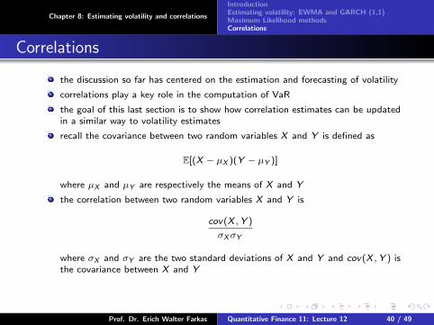
the discussion so far has centered on the estimation and forecasting of volatility
correlations play a key role in the computation of VaR
the goal of this last section is to show how correlation estimates can be updatedin a similar way to volatility estimates
recall the covariance between two random variables X and Y is defined as
E[(X − µX )(Y − µY )]
where µX and µY are respectively the means of X and Y
the correlation between two random variables X and Y is
cov(X ,Y )
σXσY
where σX and σY are the two standard deviations of X and Y and cov(X ,Y ) isthe covariance between X and Y
Prof. Dr. Erich Walter Farkas Quantitative Finance 11: Lecture 12 40 / 49

Chapter 8: Estimating volatility and correlations
IntroductionEstimating volatility: EWMA and GARCH (1,1)Maximum Likelihood methodsCorrelations
Correlations
define xi and yi as the percentage changes in X and Y between the end of theday i − 1 and the end of day i :
xi =Xi − Xi−1
Xi−1and yi =
Yi − Yi−1
Yi−1
where Xi and Yi are the values of X and Y at the end of the day i
we also define
σx,n : daily volatility of variable X estimated for day n
σy,n : daily volatility of variable Y estimated for day n
covn : estimate of covariance between daily changes in X and Y ,
calculated on day n
our estimate on the correlation between X and Y on day n is
covn
σx,nσy,n
Prof. Dr. Erich Walter Farkas Quantitative Finance 11: Lecture 12 41 / 49
Chapter 8: Estimating volatility and correlations
IntroductionEstimating volatility: EWMA and GARCH (1,1)Maximum Likelihood methodsCorrelations
Correlations
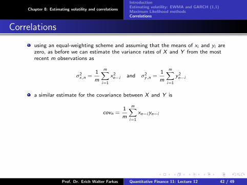
using an equal-weighting scheme and assuming that the means of xi and yi arezero, as before we can estimate the variance rates of X and Y from the mostrecent m observations as
σ2x,n =
1
m
m∑i=1
x2n−i and σ2
y,n =1
m
m∑i=1
y2n−i
a similar estimate for the covariance between X and Y is
covn =1
m
m∑i=1
xn−iyn−i
Prof. Dr. Erich Walter Farkas Quantitative Finance 11: Lecture 12 42 / 49

Chapter 8: Estimating volatility and correlations
IntroductionEstimating volatility: EWMA and GARCH (1,1)Maximum Likelihood methodsCorrelations
Correlations
one alternative for updating covariances is an EWMA model as previouslydiscussed
the formula for updating the covariance estimate is then
covn = λcovn−1 + (1− λ)xn−1yn−1
a similar analysis to that presented for the EWMA volatility model shows thatthe weights given to observations on the xi and yi decline as we move backthrough time
the lower the value of λ, the greater the weight that is given to recentobservations
Prof. Dr. Erich Walter Farkas Quantitative Finance 11: Lecture 12 43 / 49
Chapter 8: Estimating volatility and correlations
IntroductionEstimating volatility: EWMA and GARCH (1,1)Maximum Likelihood methodsCorrelations
Correlations: Example
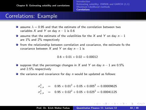
assume λ = 0.95 and that the estimate of the correlation between twovariables X and Y on day n − 1 is 0.6
assume that the estimate of the volatilities for the X and Y on day n − 1are 1% and 2% respectively
from the relationship between correlation and covariance, the estimate fo thecovariance between X and Y on day n − 1 is
0.6× 0.01× 0.02 = 0.00012
suppose that the percentage changes in X and Y on day n − 1 are 0.5%and 2.5% respectively
the variance and covariance for day n would be updated as follows:
σ2x,n = 0.95× 0.012 + 0.05× 0.0052 = 0.00009625
σ2y,n = 0.95× 0.022 + 0.05× 0.0252 = 0.00041125
Prof. Dr. Erich Walter Farkas Quantitative Finance 11: Lecture 12 44 / 49

Chapter 8: Estimating volatility and correlations
IntroductionEstimating volatility: EWMA and GARCH (1,1)Maximum Likelihood methodsCorrelations
Correlations: Example
the new volatility of X is√
0.00009625 = 0.981%
the new volatility of Y is√
0.00041125 = 2.028%
the new coefficient of correlation between X and Y is
0.00012025
0.00981× 0.02028= 0.6044
Prof. Dr. Erich Walter Farkas Quantitative Finance 11: Lecture 12 45 / 49

Chapter 8: Estimating volatility and correlations
IntroductionEstimating volatility: EWMA and GARCH (1,1)Maximum Likelihood methodsCorrelations
Correlations
GARCH models can also be used for updating covariance estimates andforecasting the future level of covariances
for example the GARCH (1,1) model for updating a covariance is
covn = ω + αxn−1yn−1 + βcovn−1
and the long-term average covariance is ω/(1− α− β)
similar formulas to those discussed above can be developed for forecastingfuture covariances and calculating the average covariance during the life time ofan option
Prof. Dr. Erich Walter Farkas Quantitative Finance 11: Lecture 12 46 / 49

Chapter 8: Estimating volatility and correlations
IntroductionEstimating volatility: EWMA and GARCH (1,1)Maximum Likelihood methodsCorrelations
Consistency condition for covariances
once all the variances and covariances have been calculated, avariance-covariance matrix can be constructed
when i 6= j , the (i , j) element of this matrix shows the covariance betweenvariable i and j ; when i = j it shows the variance of variable i
not all variance-covariance matrices are internally consistent; the condition foran N × N variance-covariance matrix Ω to be internally consistent is
wT · Ω · w ≥ 0
for all N × 1 vectors w , where wT is the transpose of w ; such a matrix is calledpositive-semidefinite
to understand why the last condition must hold, suppose that wT
is (w1, ...,wn); the expression wT · Ω · w is the variance of w1x1 + ...+ wnxnwhere xi is the value of the variable i ; as such it cannot be negative
to ensure that a positive-semidefinite matrix is produced, variances andcovariances should be calculated consistently
Prof. Dr. Erich Walter Farkas Quantitative Finance 11: Lecture 12 47 / 49

Chapter 8: Estimating volatility and correlations
IntroductionEstimating volatility: EWMA and GARCH (1,1)Maximum Likelihood methodsCorrelations
Consistency condition for covariances
to ensure that a positive-semidefinite matrix is produced, variances andcovariances should be calculated consistently
for example, if variances are calculated by giving equal weight to the last m dataitems, the same should be done for covariances
if variances are updated using an EWMA model with λ = 0.94 the same shouldbe done for covariances
an example of a variance-covariance matrix that it is not internally consistent is1 0 0.90 1 0.9
0.9 0.9 1
the variance of each variable is 1.0 and so the covariances are also coefficients ofcorrelation
the first variable is highly correlated with the third variable and the secondvariable is highly correlated with the third variable
however there is no correlation at all between the first and the second variables;this seems strange; when we set w equal to (1, 1,−1) we find that the positivesemi-definiteness condition above is not satisfied proving that the matrix is notpositive-semidefinite
Prof. Dr. Erich Walter Farkas Quantitative Finance 11: Lecture 12 48 / 49
Chapter 8: Estimating volatility and correlations
IntroductionEstimating volatility: EWMA and GARCH (1,1)Maximum Likelihood methodsCorrelations
Reference
Book:
Options, futures and other derivatives
Author: John Hull
Sixth Edition, Prentice Hall, 2006
Chapter 19: Estimating Volatilities and Correlations,pages 461 - 480
Prof. Dr. Erich Walter Farkas Quantitative Finance 11: Lecture 12 49 / 49
Top Related