


Languages
Pages
Legal

Parallel Computer Architecture and ProgrammingCMU 15-418, Spring 2013
Lecture 8:
Parallel Programming Case Studies
CMU 15-418, Spring 2013
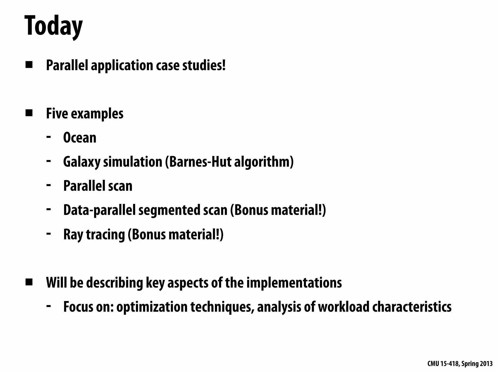
Today▪ Parallel application case studies!
▪ Five examples- Ocean- Galaxy simulation (Barnes-Hut algorithm)- Parallel scan- Data-parallel segmented scan (Bonus material!)- Ray tracing (Bonus material!)
▪ Will be describing key aspects of the implementations- Focus on: optimization techniques, analysis of workload characteristics
CMU 15-418, Spring 2013
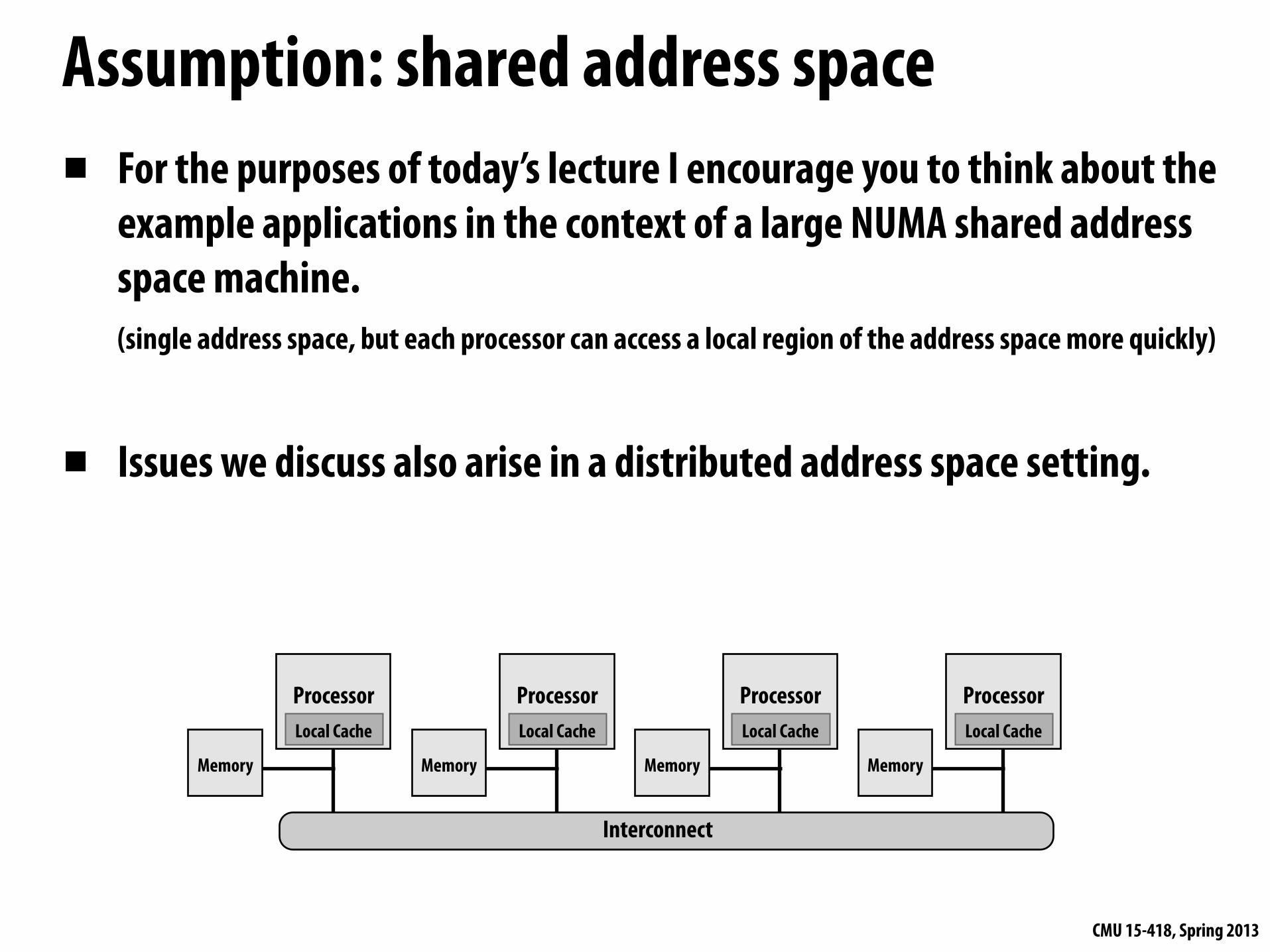
Assumption: shared address space▪ For the purposes of today’s lecture I encourage you to think about the
example applications in the context of a large NUMA shared address space machine.(single address space, but each processor can access a local region of the address space more quickly)
▪ Issues we discuss also arise in a distributed address space setting.
ProcessorLocal Cache
Memory
ProcessorLocal Cache
Memory
ProcessorLocal Cache
Memory
ProcessorLocal Cache
Memory
Interconnect
CMU 15-418, Spring 2013
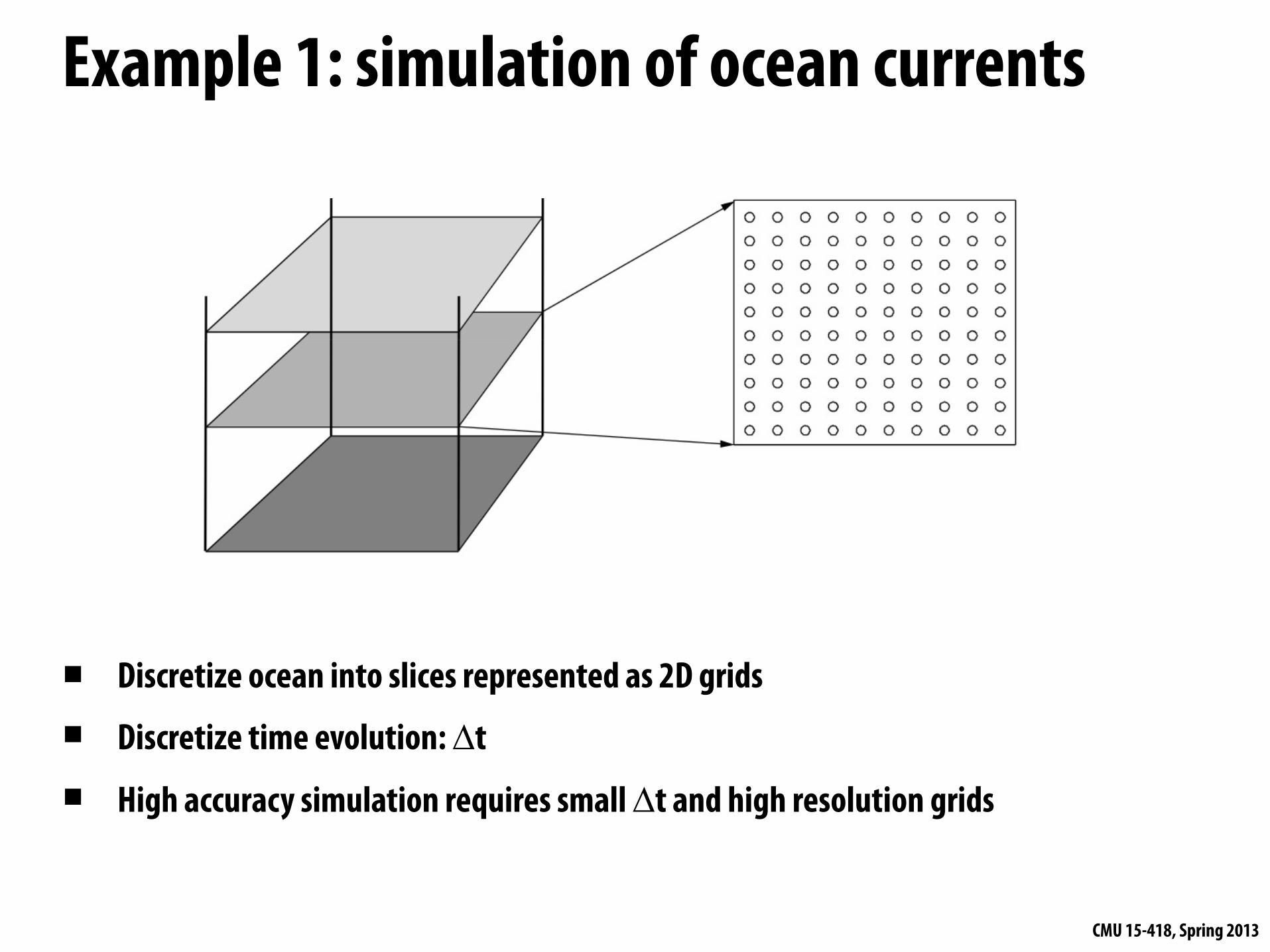
Example 1: simulation of ocean currents
▪ Discretize ocean into slices represented as 2D grids
▪ Discretize time evolution: ∆t
▪ High accuracy simulation requires small ∆t and high resolution grids
CMU 15-418, Spring 2013
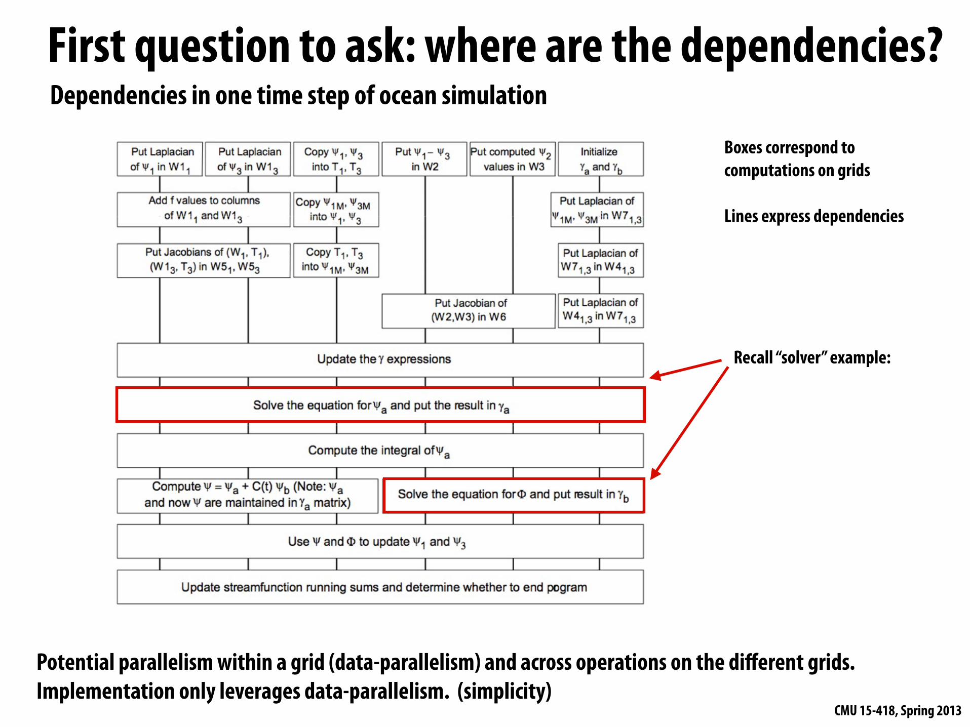
First question to ask: where are the dependencies?
Potential parallelism within a grid (data-parallelism) and across operations on the different grids. Implementation only leverages data-parallelism. (simplicity)
Boxes correspond to computations on grids
Lines express dependencies
Recall “solver” example:
Dependencies in one time step of ocean simulation
CMU 15-418, Spring 2013
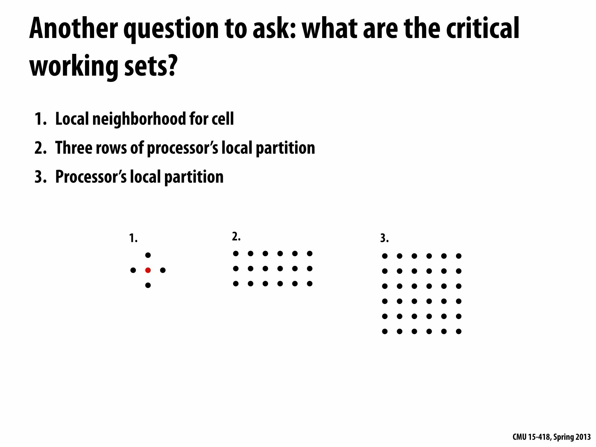
Another question to ask: what are the critical working sets?1. Local neighborhood for cell2. Three rows of processor’s local partition3. Processor’s local partition
1. 2. 3.
CMU 15-418, Spring 2013
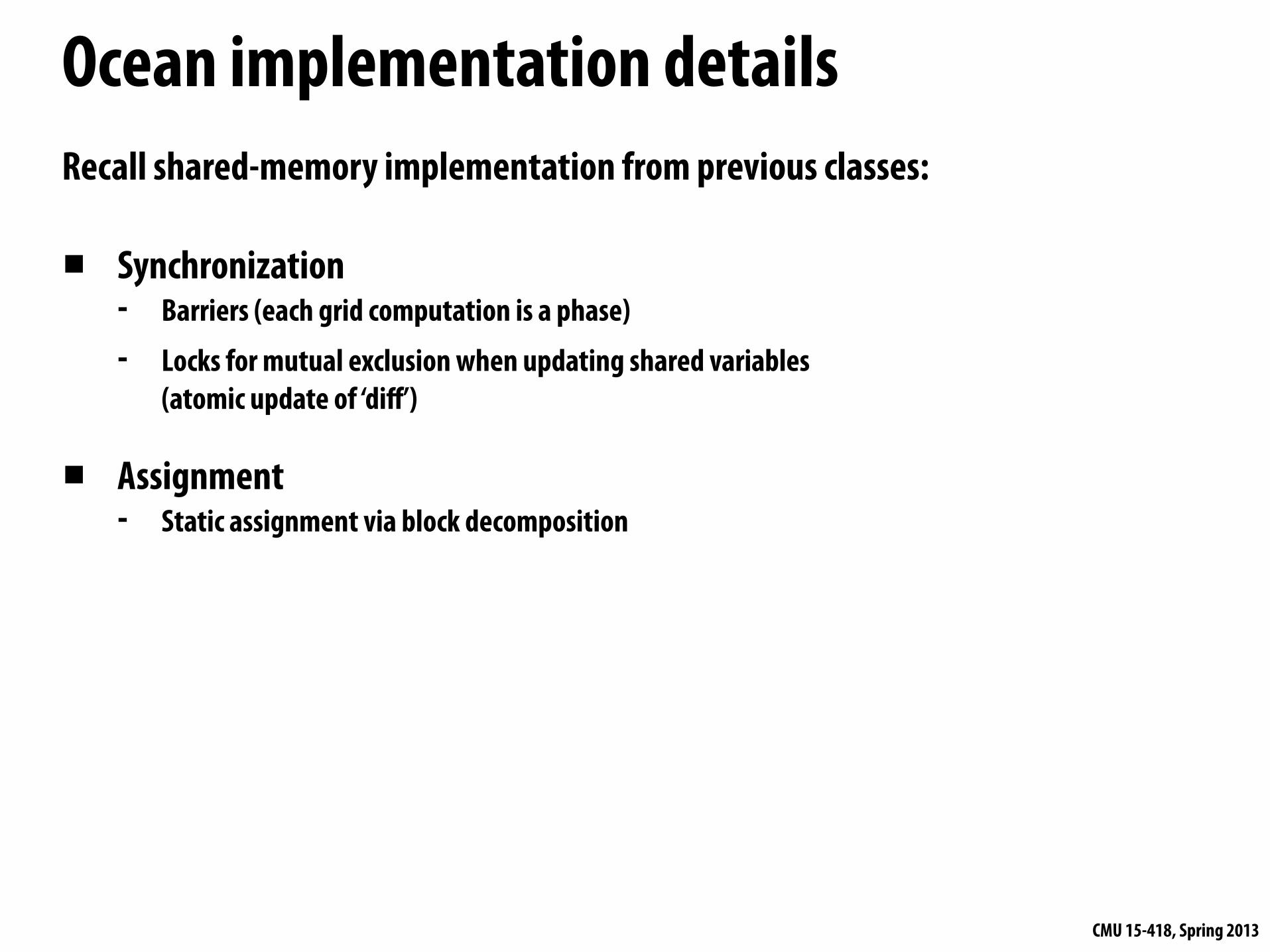
Recall shared-memory implementation from previous classes:
▪ Synchronization- Barriers (each grid computation is a phase)- Locks for mutual exclusion when updating shared variables
(atomic update of ‘diff’)
▪ Assignment- Static assignment via block decomposition
Ocean implementation details
CMU 15-418, Spring 2013
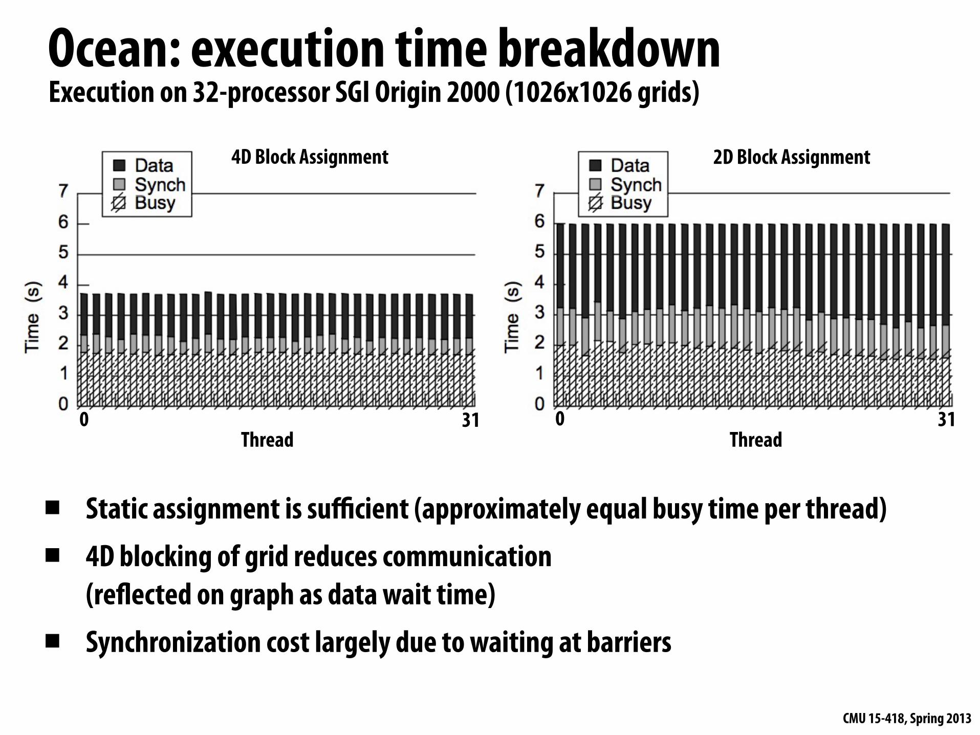
Ocean: execution time breakdown
Thread Thread0 31 0 31
▪ Static assignment is sufficient (approximately equal busy time per thread)▪ 4D blocking of grid reduces communication
(re"ected on graph as data wait time)▪ Synchronization cost largely due to waiting at barriers
4D Block Assignment 2D Block Assignment
Execution on 32-processor SGI Origin 2000 (1026x1026 grids)
CMU 15-418, Spring 2013
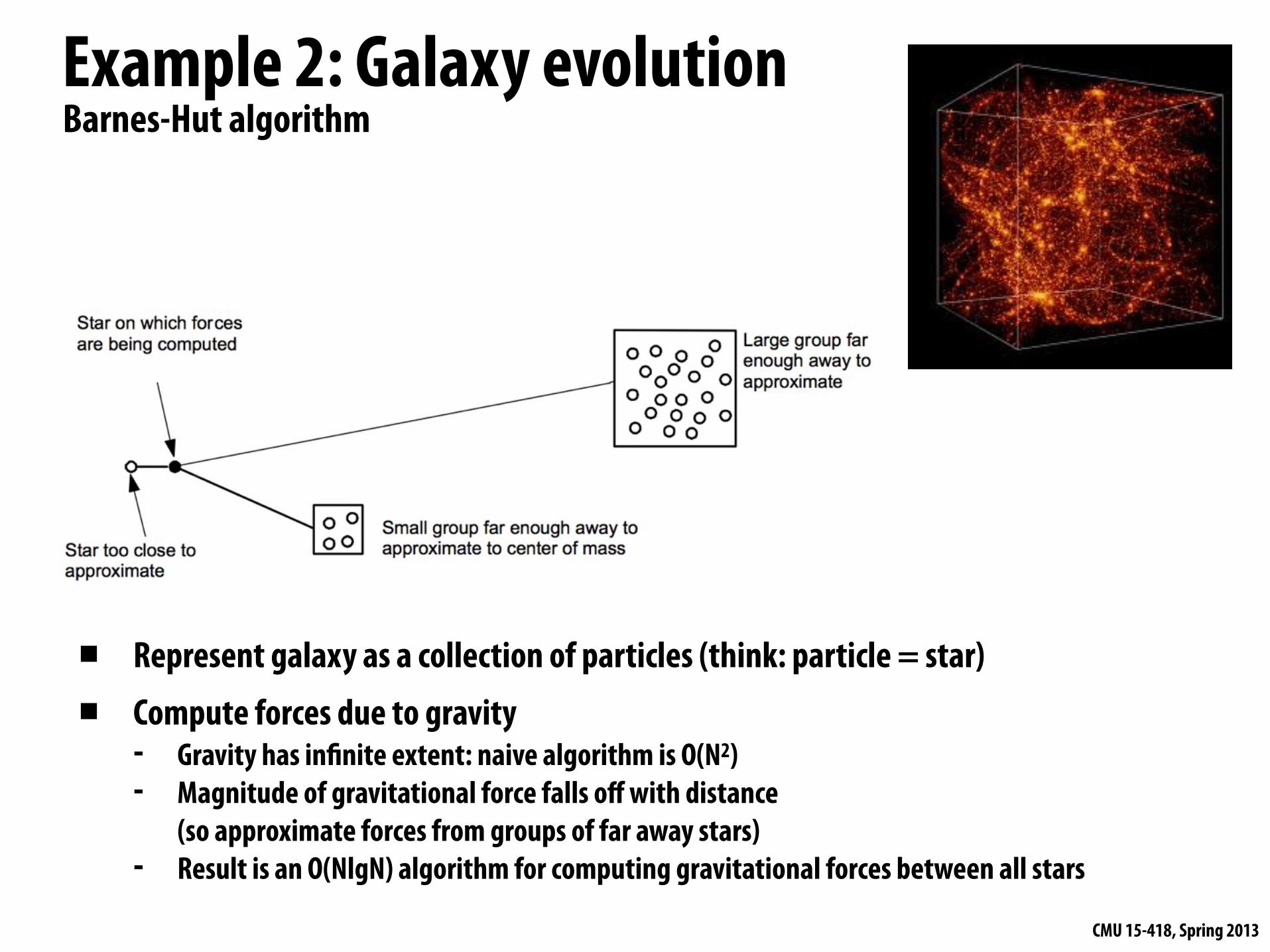
Example 2: Galaxy evolution
▪ Represent galaxy as a collection of particles (think: particle = star)
▪ Compute forces due to gravity- Gravity has in"nite extent: naive algorithm is O(N2)- Magnitude of gravitational force falls off with distance
(so approximate forces from groups of far away stars)- Result is an O(NlgN) algorithm for computing gravitational forces between all stars
Barnes-Hut algorithm
CMU 15-418, Spring 2013
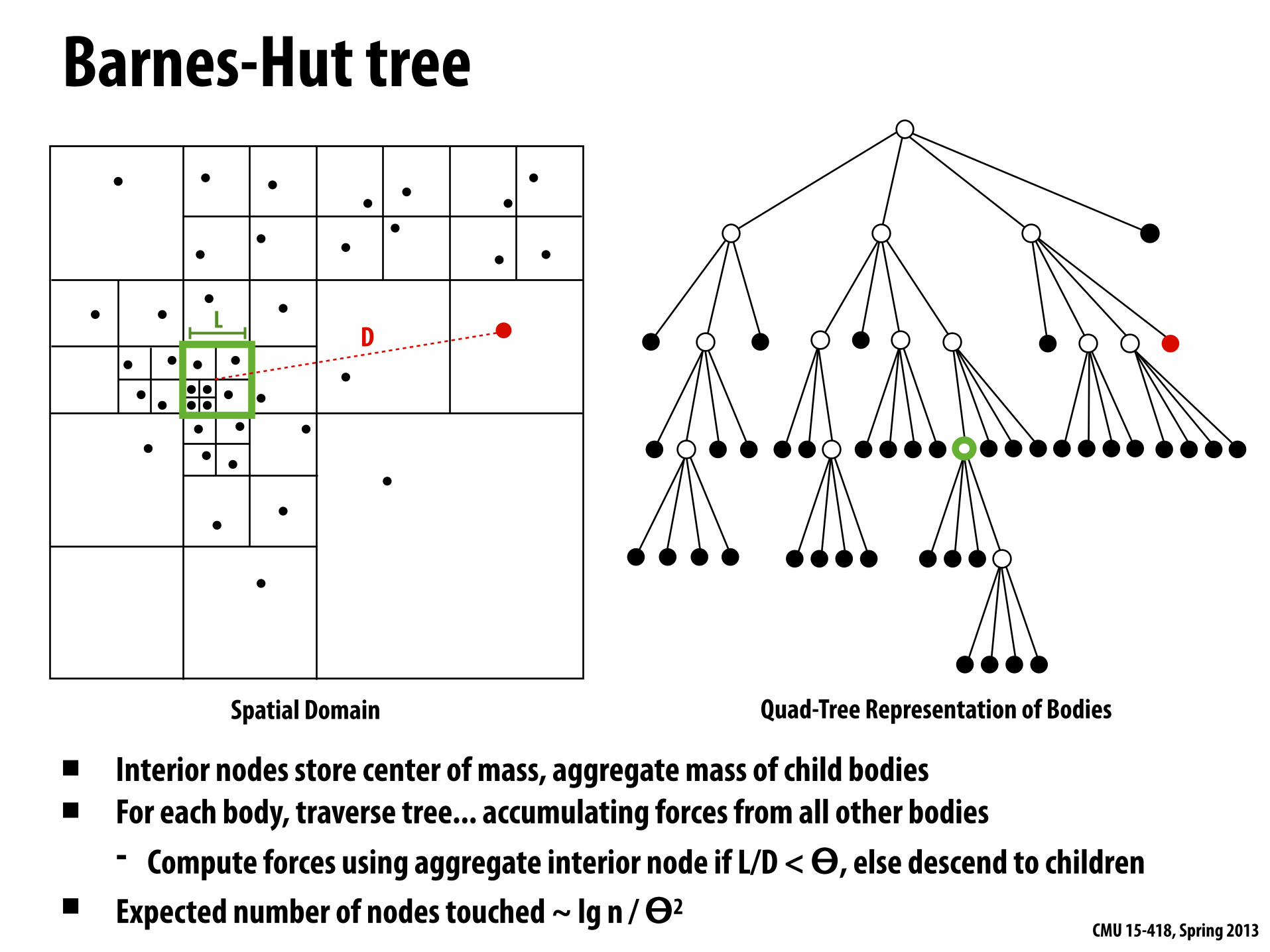
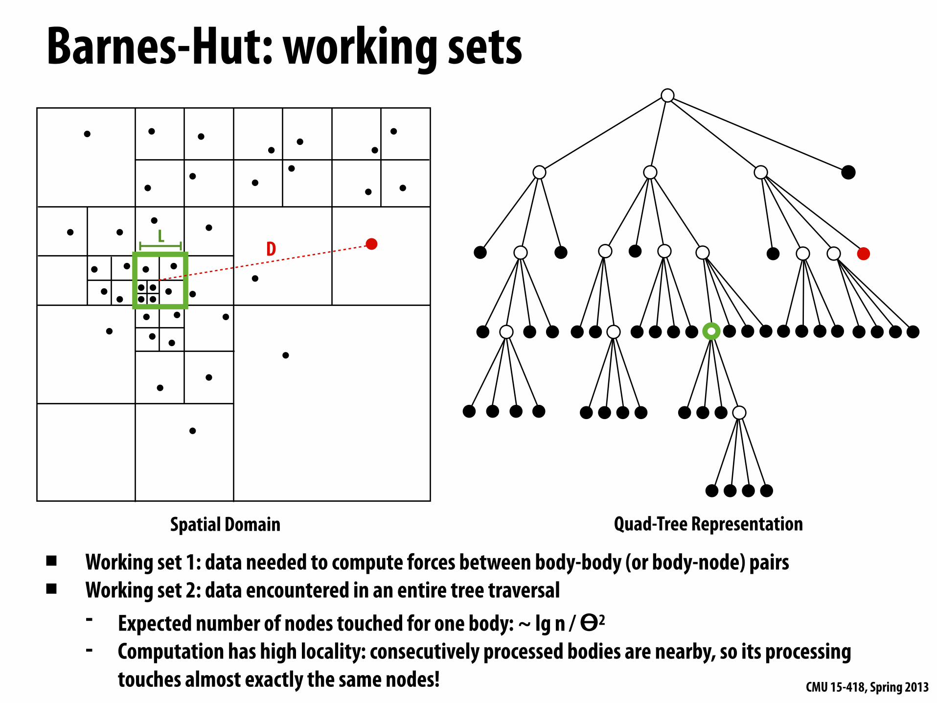
Barnes-Hut tree
Spatial Domain Quad-Tree Representation of Bodies
▪ Interior nodes store center of mass, aggregate mass of child bodies▪ For each body, traverse tree... accumulating forces from all other bodies
- Compute forces using aggregate interior node if L/D < ϴ, else descend to children▪ Expected number of nodes touched ~ lg n / ϴ2
LD
CMU 15-418, Spring 2013
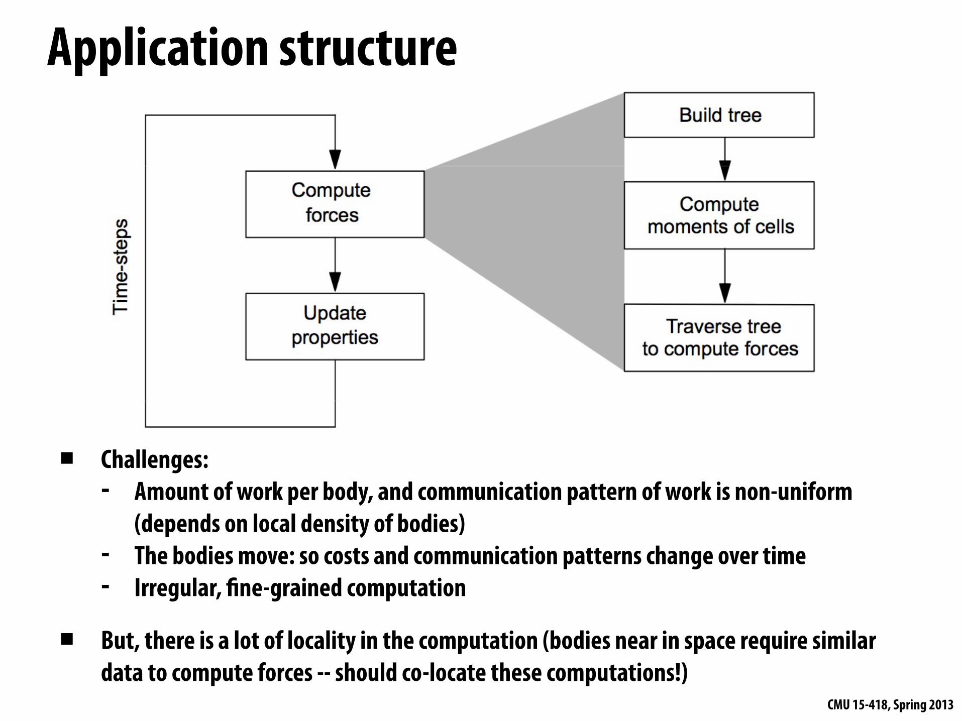
Application structure
▪ Challenges:- Amount of work per body, and communication pattern of work is non-uniform
(depends on local density of bodies)- The bodies move: so costs and communication patterns change over time- Irregular, !ne-grained computation
▪ But, there is a lot of locality in the computation (bodies near in space require similar data to compute forces -- should co-locate these computations!)
CMU 15-418, Spring 2013
Work assignment▪ Challenge:
- Equal number of bodies per processor != equal work per processor- Want equal work per processor AND assignment should preserve locality
▪ Observation: spatial distribution of bodies evolves slowly
▪ Use semi-static assignment - Each time step, for each body, record number of interactions with other
bodies (the application pro#les itself)- Cheap to compute. Just increment local per-body counters- Use values to periodically recompute assignment
CMU 15-418, Spring 2013
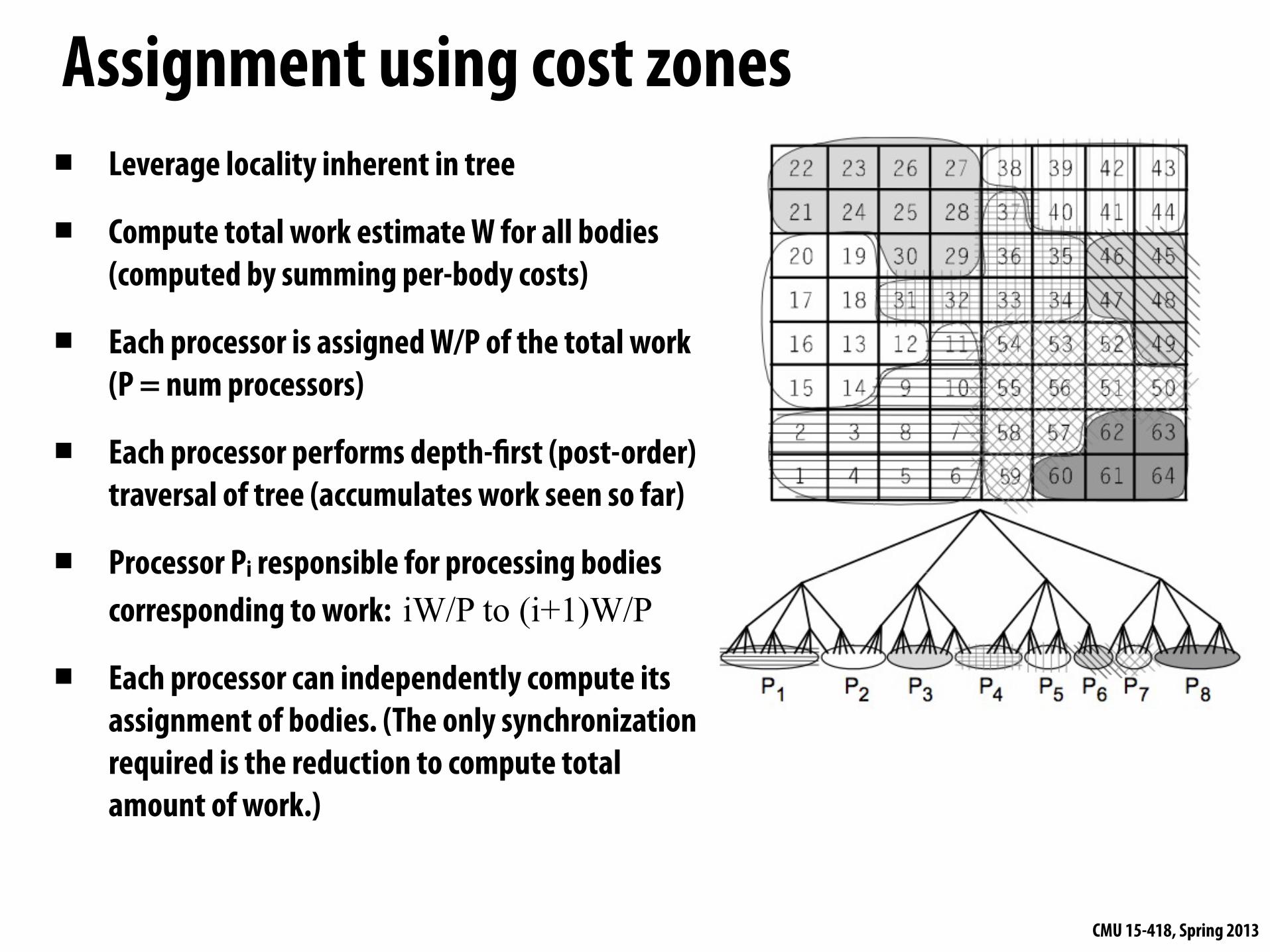
Assignment using cost zones▪ Leverage locality inherent in tree
▪ Compute total work estimate W for all bodies(computed by summing per-body costs)
▪ Each processor is assigned W/P of the total work (P = num processors)
▪ Each processor performs depth-!rst (post-order) traversal of tree (accumulates work seen so far)
▪ Processor Pi responsible for processing bodies corresponding to work: iW/P to (i+1)W/P
▪ Each processor can independently compute its assignment of bodies. (The only synchronization required is the reduction to compute total amount of work.)
CMU 15-418, Spring 2013
Barnes-Hut: working sets
Spatial Domain Quad-Tree Representation
▪ Working set 1: data needed to compute forces between body-body (or body-node) pairs▪ Working set 2: data encountered in an entire tree traversal
- Expected number of nodes touched for one body: ~ lg n / ϴ2
- Computation has high locality: consecutively processed bodies are nearby, so its processing touches almost exactly the same nodes!
LD
CMU 15-418, Spring 2013
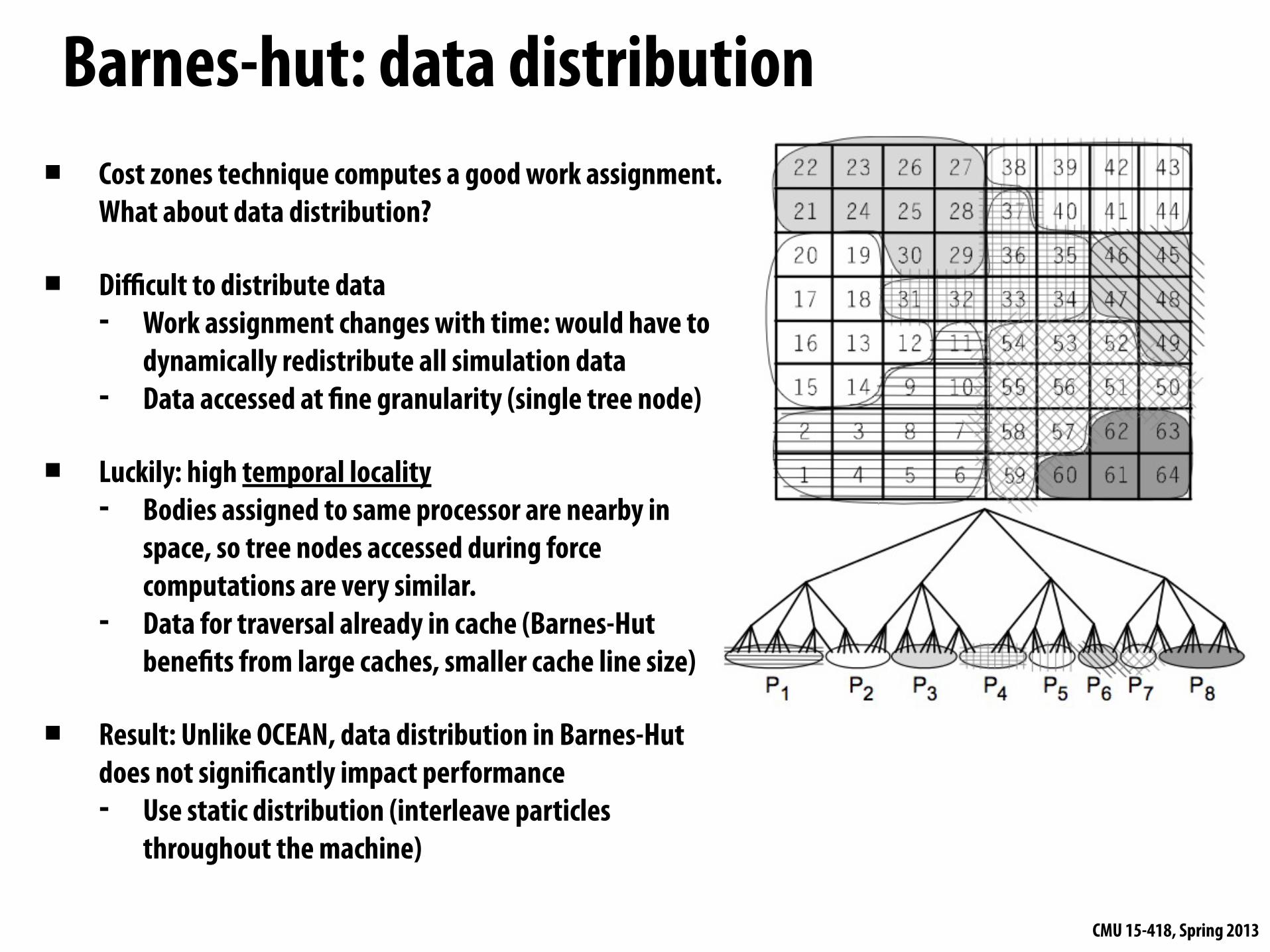
Barnes-hut: data distribution▪ Cost zones technique computes a good work assignment.
What about data distribution?
▪ Difficult to distribute data- Work assignment changes with time: would have to
dynamically redistribute all simulation data- Data accessed at "ne granularity (single tree node)
▪ Luckily: high temporal locality- Bodies assigned to same processor are nearby in
space, so tree nodes accessed during force computations are very similar.
- Data for traversal already in cache (Barnes-Hut bene"ts from large caches, smaller cache line size)
▪ Result: Unlike OCEAN, data distribution in Barnes-Hut does not signi"cantly impact performance- Use static distribution (interleave particles
throughout the machine)
CMU 15-418, Spring 2013
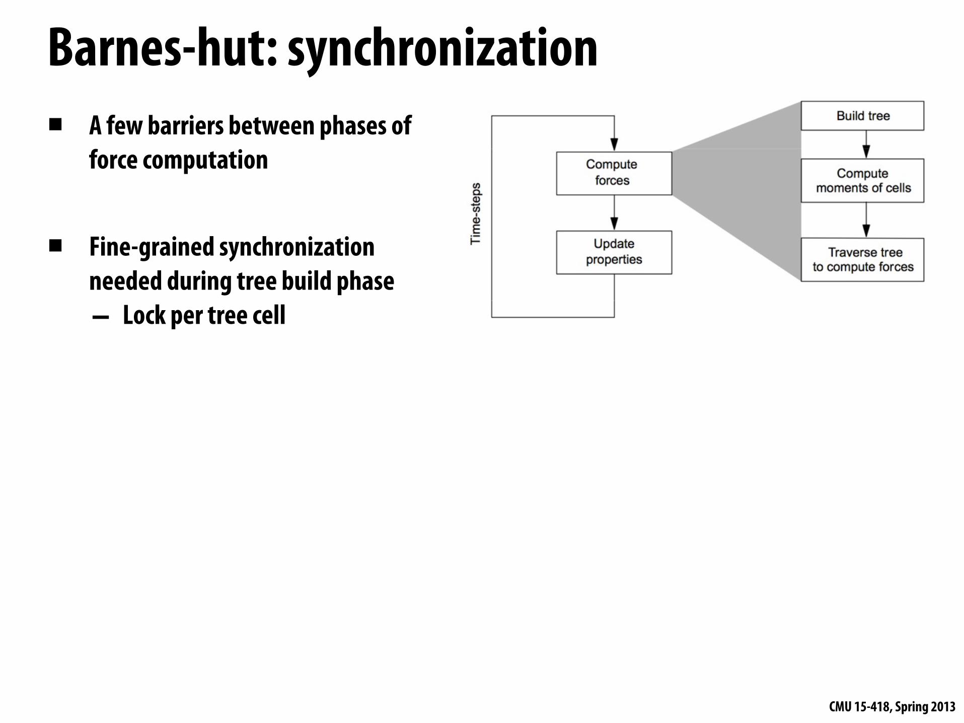
Barnes-hut: synchronization▪ A few barriers between phases of
force computation
▪ Fine-grained synchronization needed during tree build phase- Lock per tree cell
CMU 15-418, Spring 2013
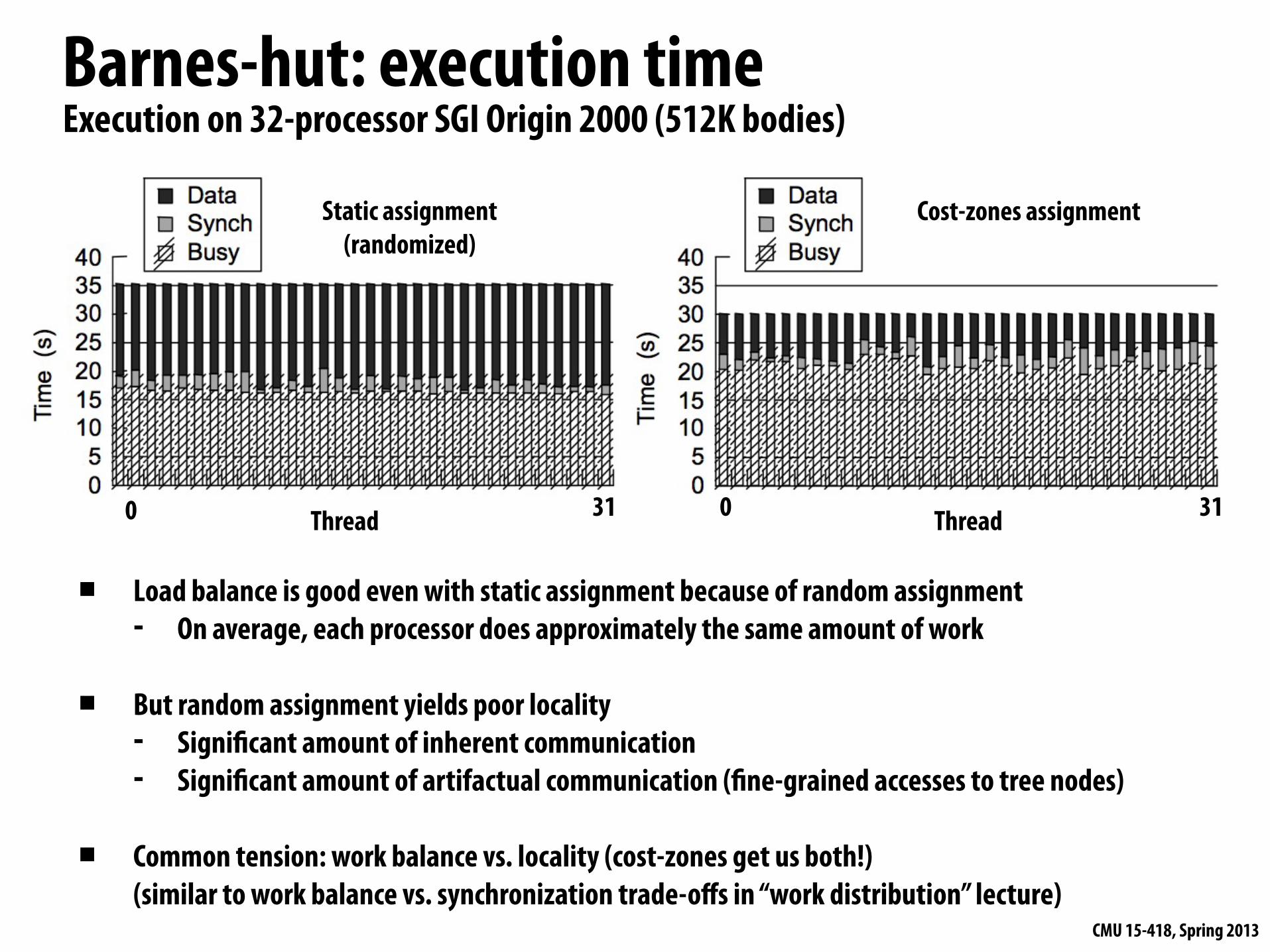
Barnes-hut: execution time
Thread Thread0 31 0 31
Static assignment(randomized)
Cost-zones assignment
Execution on 32-processor SGI Origin 2000 (512K bodies)
▪ Load balance is good even with static assignment because of random assignment- On average, each processor does approximately the same amount of work
▪ But random assignment yields poor locality- Signi"cant amount of inherent communication- Signi"cant amount of artifactual communication ("ne-grained accesses to tree nodes)
▪ Common tension: work balance vs. locality (cost-zones get us both!)(similar to work balance vs. synchronization trade-offs in “work distribution” lecture)
CMU 15-418, Spring 2013
Summary▪ Today so far: two examples of parallel program optimization▪ Key issues when discussing the applications
- How to balance the work?- How to exploit locality inherent in the problem?- What synchronization is necessary?
CMU 15-418, Spring 2013
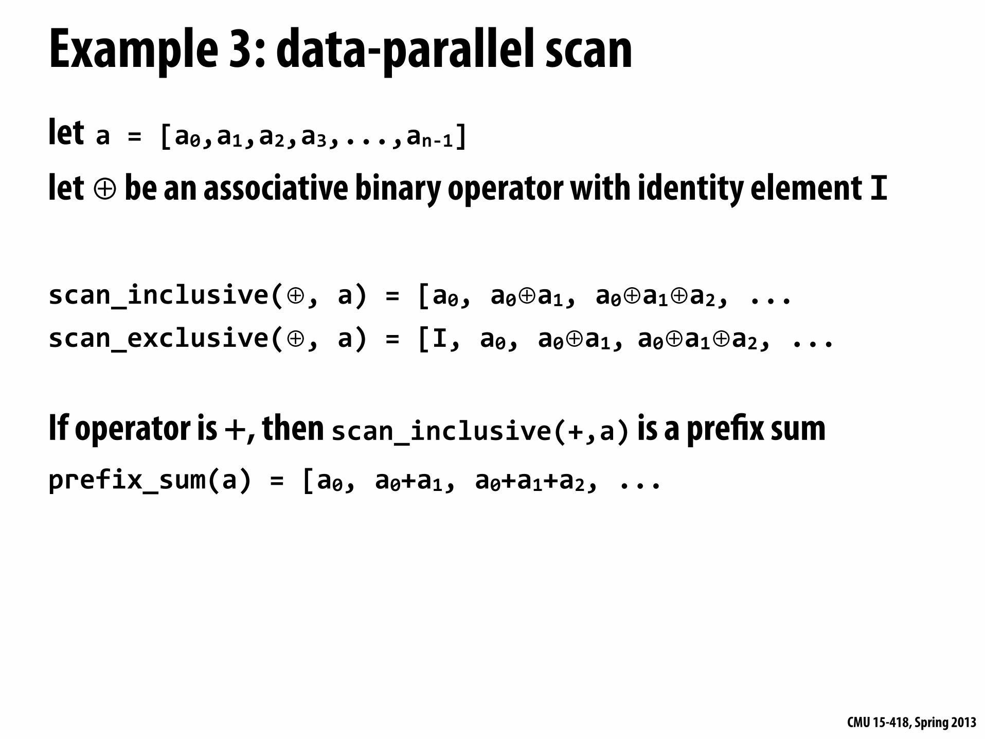
Example 3: data-parallel scanlet a = [a0,a1,a2,a3,...,an-‐1]let ⊕ be an associative binary operator with identity element I
scan_inclusive(⊕, a) = [a0, a0⊕a1, a0⊕a1⊕a2, ...scan_exclusive(⊕, a) = [I, a0, a0⊕a1, a0⊕a1⊕a2, ...
If operator is +, then scan_inclusive(+,a) is a pre#x sumprefix_sum(a) = [a0, a0+a1, a0+a1+a2, ...
CMU 15-418, Spring 2013
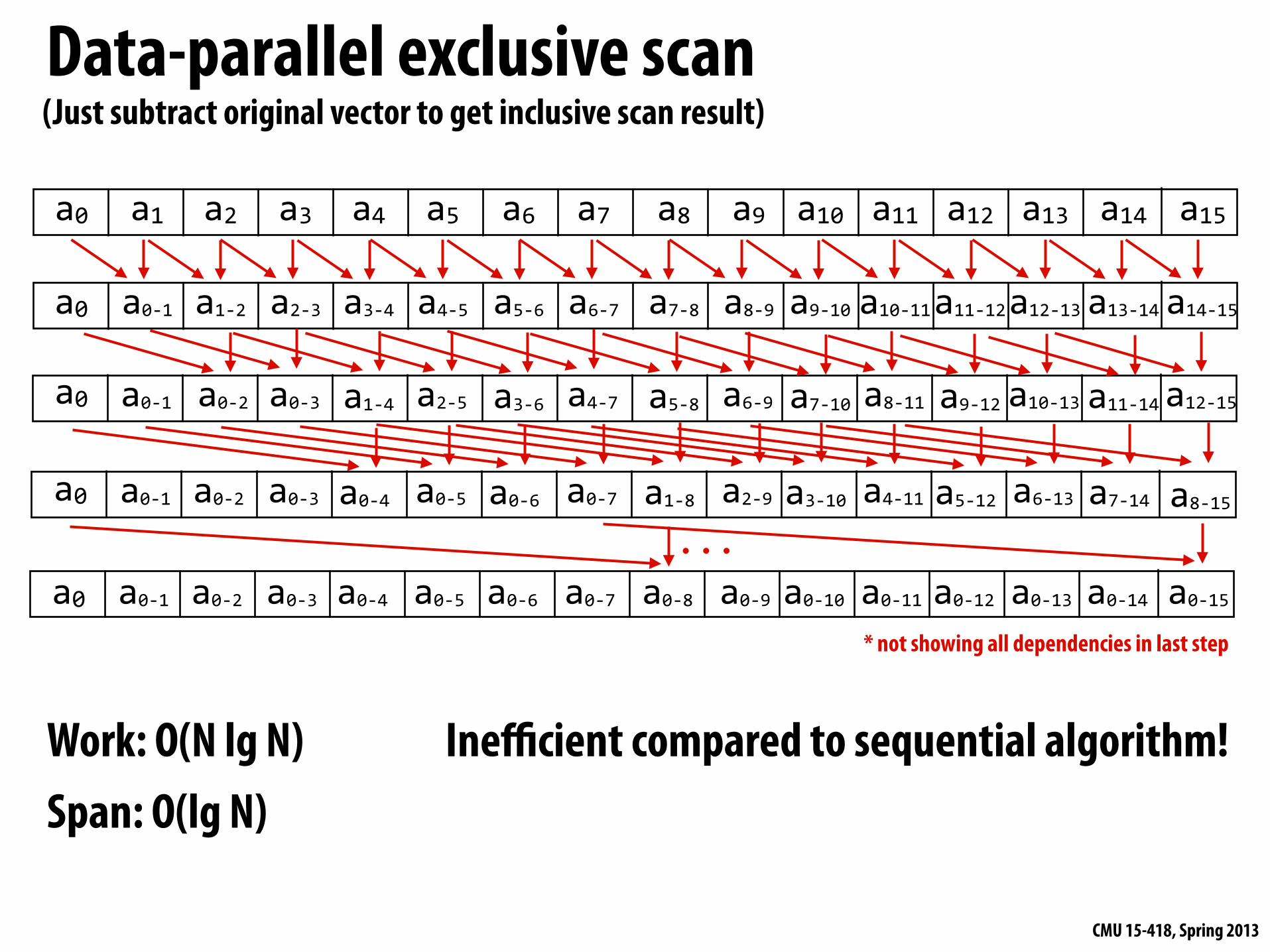
Data-parallel exclusive scan
a0 a1 a2 a3 a4 a5 a6 a7 a8 a9 a10 a11 a12 a13 a14 a15
a0 a0-‐1 a1-‐2 a2-‐3 a3-‐4 a4-‐5 a5-‐6 a6-‐7 a7-‐8 a8-‐9 a9-‐10 a10-‐11a11-‐12a12-‐13 a13-‐14 a14-‐15
a0-‐1 a0-‐3 a2-‐5 a4-‐7 a6-‐9 a8-‐11 a10-‐13 a12-‐15a0-‐2 a1-‐4 a3-‐6 a5-‐8 a7-‐10 a9-‐12 a11-‐14a0
a0-‐1 a0-‐3 a0-‐5 a0-‐7 a2-‐9 a4-‐11 a6-‐13 a8-‐15a0 a0-‐2 a0-‐4 a0-‐6 a1-‐8 a3-‐10 a5-‐12 a7-‐14
a0-‐1 a0-‐3 a0-‐5 a0-‐7 a0-‐9 a0-‐11 a0-‐13 a0-‐15a0 a0-‐2 a0-‐4 a0-‐6 a0-‐8 a0-‐10 a0-‐12 a0-‐14
...
* not showing all dependencies in last step
(Just subtract original vector to get inclusive scan result)
Work: O(N lg N) Inefficient compared to sequential algorithm!Span: O(lg N)
CMU 15-418, Spring 2013
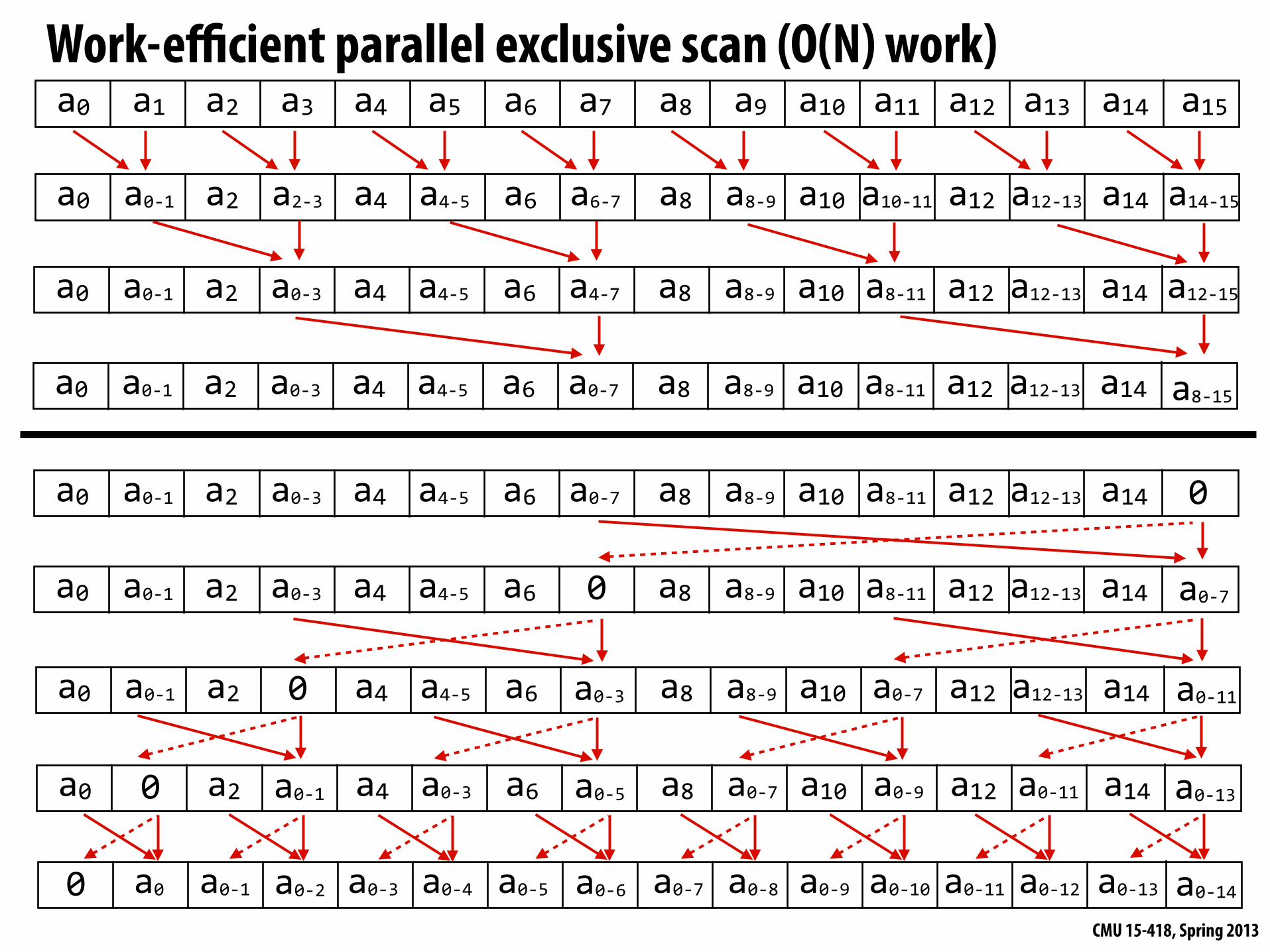
Work-efficient parallel exclusive scan (O(N) work) a0 a1 a2 a3 a4 a5 a6 a7 a8 a9 a10 a11 a12 a13 a14 a15
a0 a0-‐1 a2 a2-‐3 a4 a4-‐5 a6 a6-‐7 a8 a8-‐9 a10 a10-‐11 a12 a12-‐13 a14 a14-‐15
a0 a0-‐1 a2 a0-‐3 a4 a4-‐5 a6 a4-‐7 a8 a8-‐9 a10 a8-‐11 a12 a12-‐13 a14 a12-‐15
a0 a0-‐1 a2 a0-‐3 a4 a4-‐5 a6 a0-‐7 a8 a8-‐9 a10 a8-‐11 a12 a12-‐13 a14 a8-‐15
a0 a0-‐1 a2 a0-‐3 a4 a4-‐5 a6 a0-‐7 a8 a8-‐9 a10 a8-‐11 a12 a12-‐13 a14 0
a0 a0-‐1 a2 a0-‐3 a4 a4-‐5 a6 0 a8 a8-‐9 a10 a8-‐11 a12 a12-‐13 a14 a0-‐7
a0 a0-‐1 a2 0 a4 a4-‐5 a6 a0-‐3 a8 a8-‐9 a10 a0-‐7 a12 a12-‐13 a14 a0-‐11
a0 0 a2 a0-‐1 a4 a0-‐3 a6 a0-‐5 a8 a0-‐7 a10 a0-‐9 a12 a0-‐11 a14 a0-‐13
a00 a0-‐1 a0-‐2 a0-‐3 a0-‐4 a0-‐5 a0-‐6 a0-‐7 a0-‐8 a0-‐9 a0-‐10 a0-‐11 a0-‐12 a0-‐13 a0-‐14
CMU 15-418, Spring 2013
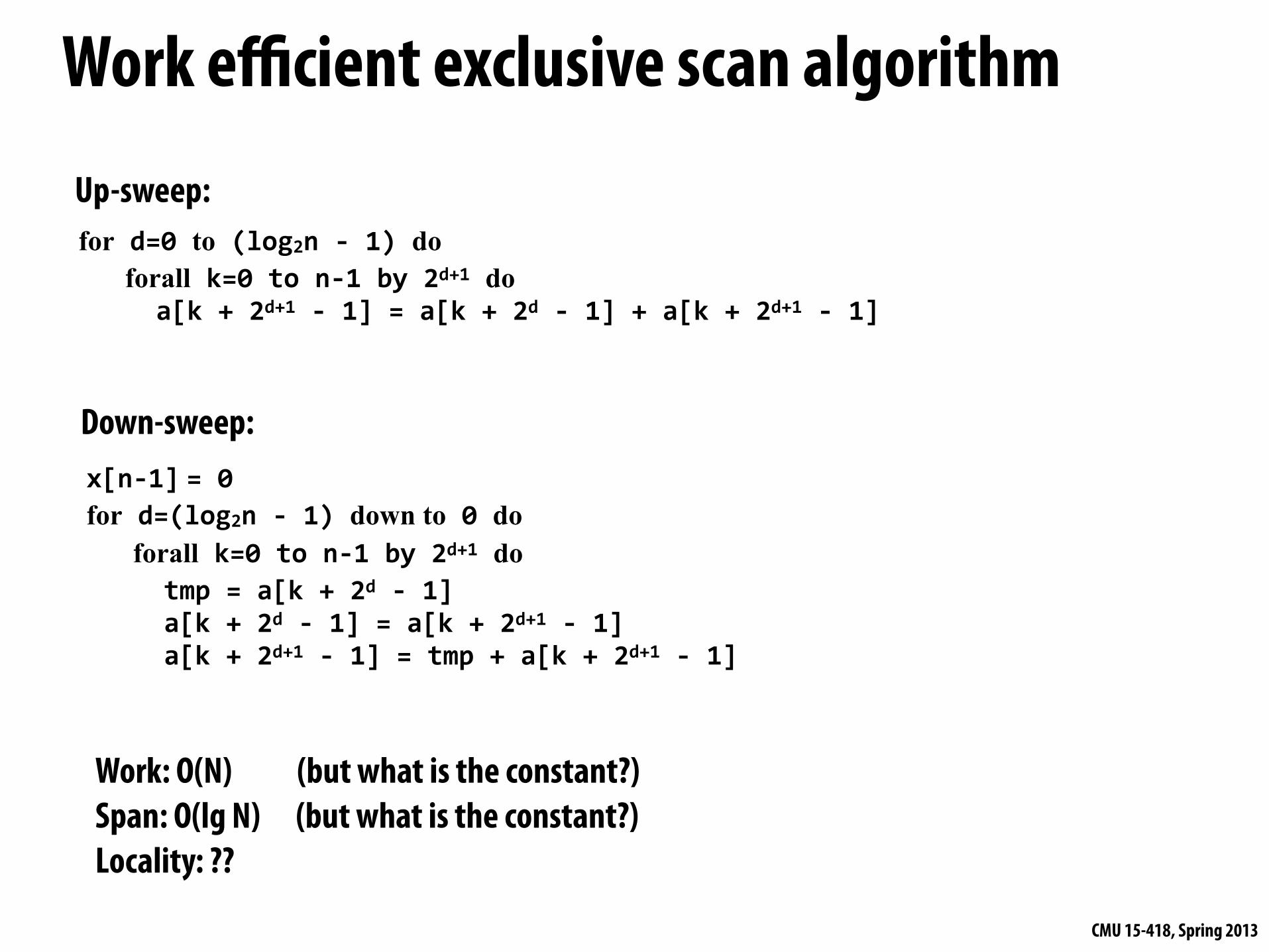
Work efficient exclusive scan algorithm
for d=0 to (log2n -‐ 1) do forall k=0 to n-‐1 by 2d+1 do a[k + 2d+1 -‐ 1] = a[k + 2d -‐ 1] + a[k + 2d+1 -‐ 1]
x[n-‐1] = 0for d=(log2n -‐ 1) down to 0 do forall k=0 to n-‐1 by 2d+1 do tmp = a[k + 2d -‐ 1] a[k + 2d -‐ 1] = a[k + 2d+1 -‐ 1] a[k + 2d+1 -‐ 1] = tmp + a[k + 2d+1 -‐ 1]
Down-sweep:
Up-sweep:
Work: O(N) (but what is the constant?)Span: O(lg N) (but what is the constant?)Locality: ??
CMU 15-418, Spring 2013
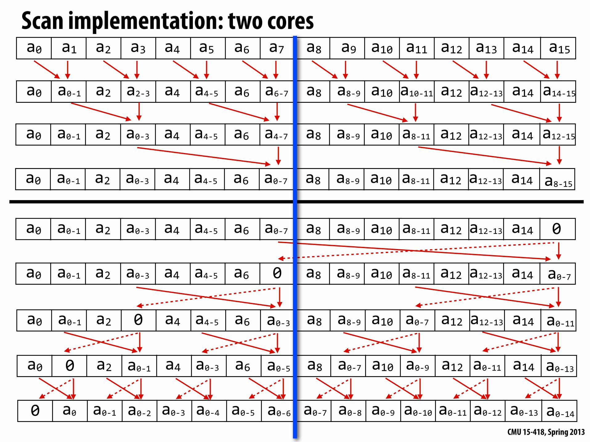
Scan implementation: two coresa0 a1 a2 a3 a4 a5 a6 a7 a8 a9 a10 a11 a12 a13 a14 a15
a0 a0-‐1 a2 a2-‐3 a4 a4-‐5 a6 a6-‐7 a8 a8-‐9 a10 a10-‐11 a12 a12-‐13 a14 a14-‐15
a0 a0-‐1 a2 a0-‐3 a4 a4-‐5 a6 a4-‐7 a8 a8-‐9 a10 a8-‐11 a12 a12-‐13 a14 a12-‐15
a0 a0-‐1 a2 a0-‐3 a4 a4-‐5 a6 a0-‐7 a8 a8-‐9 a10 a8-‐11 a12 a12-‐13 a14 a8-‐15
a0 a0-‐1 a2 a0-‐3 a4 a4-‐5 a6 a0-‐7 a8 a8-‐9 a10 a8-‐11 a12 a12-‐13 a14 0
a0 a0-‐1 a2 a0-‐3 a4 a4-‐5 a6 0 a8 a8-‐9 a10 a8-‐11 a12 a12-‐13 a14 a0-‐7
a0 a0-‐1 a2 0 a4 a4-‐5 a6 a0-‐3 a8 a8-‐9 a10 a0-‐7 a12 a12-‐13 a14 a0-‐11
a0 0 a2 a0-‐1 a4 a0-‐3 a6 a0-‐5 a8 a0-‐7 a10 a0-‐9 a12 a0-‐11 a14 a0-‐13
a00 a0-‐1 a0-‐2 a0-‐3 a0-‐4 a0-‐5 a0-‐6 a0-‐7 a0-‐8 a0-‐9 a0-‐10 a0-‐11 a0-‐12 a0-‐13 a0-‐14
CMU 15-418, Spring 2013
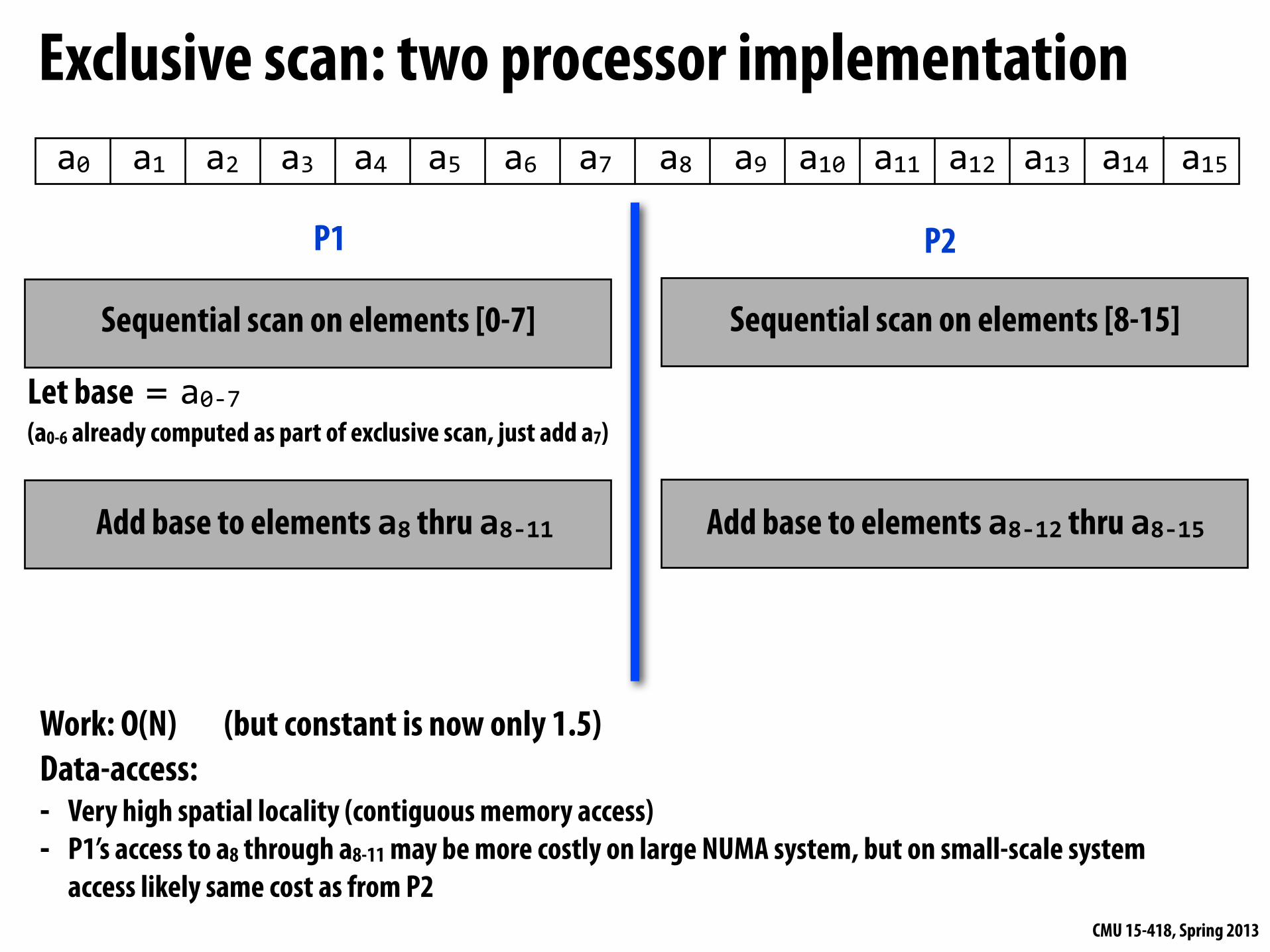
Exclusive scan: two processor implementationa0 a1 a2 a3 a4 a5 a6 a7 a8 a9 a10 a11 a12 a13 a14 a15
Sequential scan on elements [0-7] Sequential scan on elements [8-15]
Add base to elements a8 thru a8-‐11 Add base to elements a8-‐12 thru a8-‐15
P1 P2
Let base = a0-‐7(a0-6 already computed as part of exclusive scan, just add a7)
Work: O(N) (but constant is now only 1.5)Data-access:- Very high spatial locality (contiguous memory access)- P1’s access to a8 through a8-11 may be more costly on large NUMA system, but on small-scale system
access likely same cost as from P2
CMU 15-418, Spring 2013
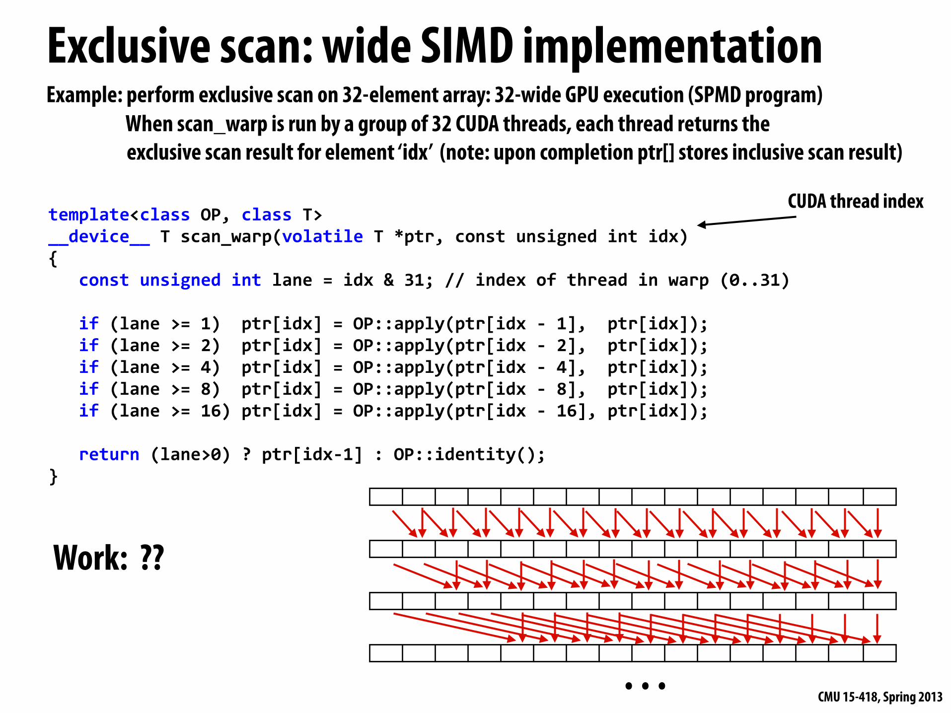
Exclusive scan: wide SIMD implementationExample: perform exclusive scan on 32-element array: 32-wide GPU execution (SPMD program) When scan_warp is run by a group of 32 CUDA threads, each thread returns the
exclusive scan result for element ‘idx’ (note: upon completion ptr[] stores inclusive scan result)
template<class OP, class T>__device__ T scan_warp(volatile T *ptr, const unsigned int idx){ const unsigned int lane = idx & 31; // index of thread in warp (0..31)
if (lane >= 1) ptr[idx] = OP::apply(ptr[idx -‐ 1], ptr[idx]); if (lane >= 2) ptr[idx] = OP::apply(ptr[idx -‐ 2], ptr[idx]); if (lane >= 4) ptr[idx] = OP::apply(ptr[idx -‐ 4], ptr[idx]); if (lane >= 8) ptr[idx] = OP::apply(ptr[idx -‐ 8], ptr[idx]); if (lane >= 16) ptr[idx] = OP::apply(ptr[idx -‐ 16], ptr[idx]);
return (lane>0) ? ptr[idx-‐1] : OP::identity();}
CUDA thread index
. . .
Work: ??
CMU 15-418, Spring 2013
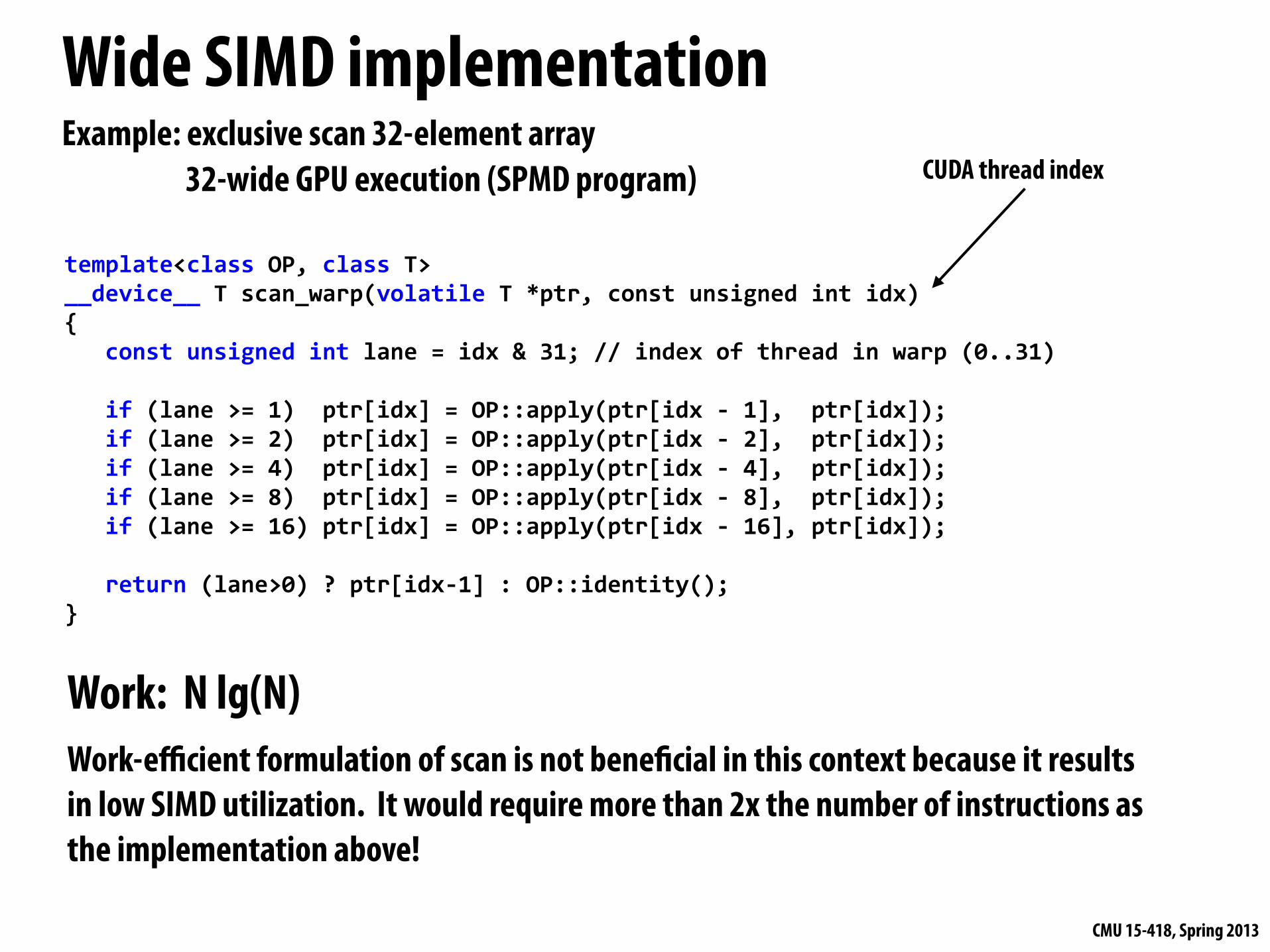
Wide SIMD implementationExample: exclusive scan 32-element array 32-wide GPU execution (SPMD program)
template<class OP, class T>__device__ T scan_warp(volatile T *ptr, const unsigned int idx){ const unsigned int lane = idx & 31; // index of thread in warp (0..31)
if (lane >= 1) ptr[idx] = OP::apply(ptr[idx -‐ 1], ptr[idx]); if (lane >= 2) ptr[idx] = OP::apply(ptr[idx -‐ 2], ptr[idx]); if (lane >= 4) ptr[idx] = OP::apply(ptr[idx -‐ 4], ptr[idx]); if (lane >= 8) ptr[idx] = OP::apply(ptr[idx -‐ 8], ptr[idx]); if (lane >= 16) ptr[idx] = OP::apply(ptr[idx -‐ 16], ptr[idx]);
return (lane>0) ? ptr[idx-‐1] : OP::identity();}
CUDA thread index
Work: N lg(N)Work-efficient formulation of scan is not bene#cial in this context because it results in low SIMD utilization. It would require more than 2x the number of instructions as the implementation above!
CMU 15-418, Spring 2013
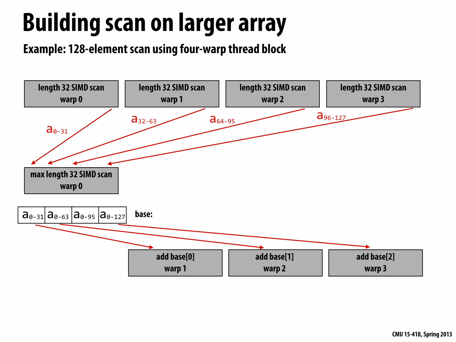
Building scan on larger array
length 32 SIMD scanwarp 0
length 32 SIMD scanwarp 1
length 32 SIMD scanwarp 2
length 32 SIMD scanwarp 3
Example: 128-element scan using four-warp thread block
max length 32 SIMD scanwarp 0
a0-‐31
a32-‐63 a64-‐95a96-‐127
add base[0]warp 1
a0-‐31 a0-‐63 a0-‐95 a0-‐127
add base[1]warp 2
add base[2]warp 3
base:
CMU 15-418, Spring 2013
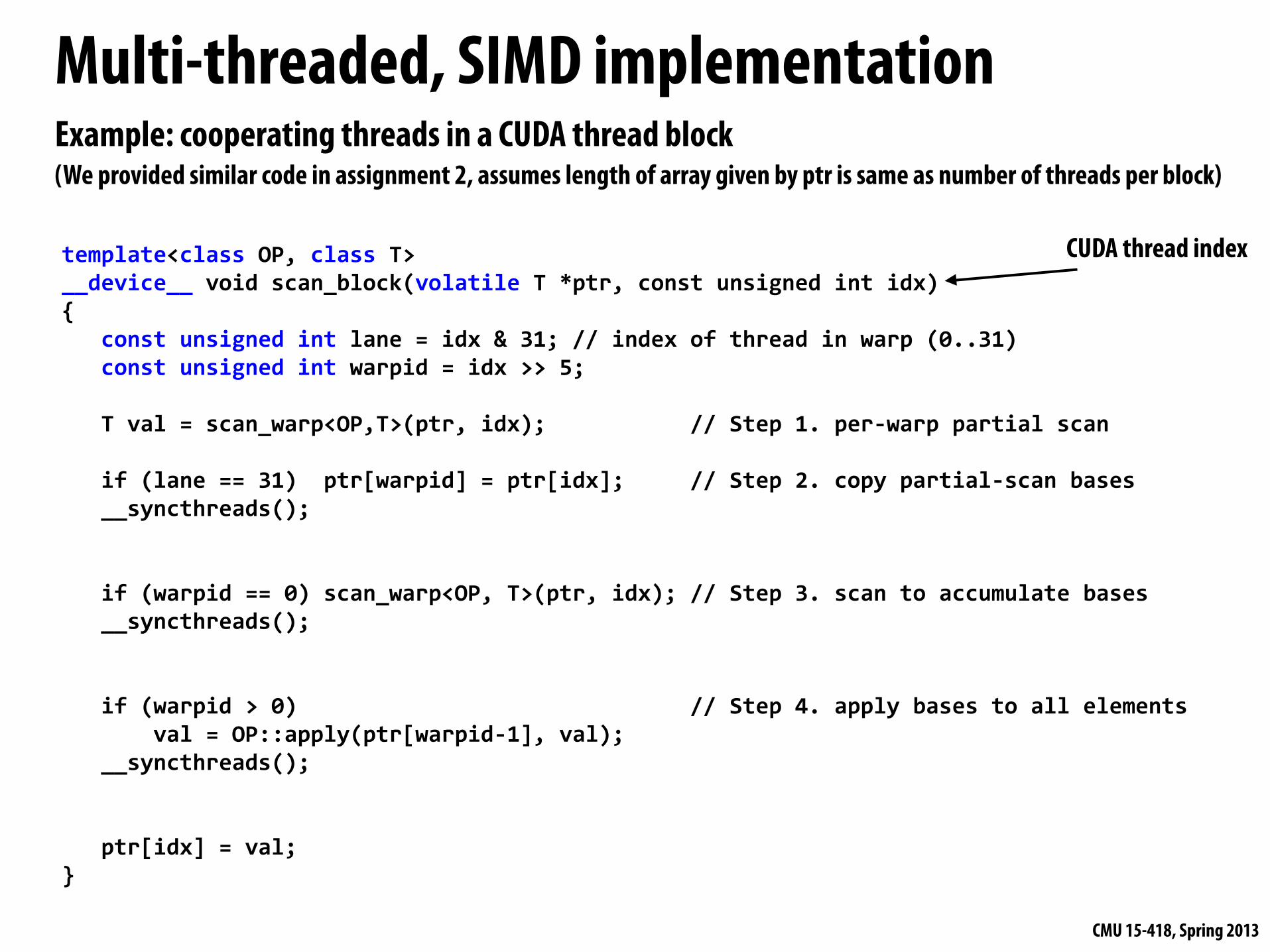
Multi-threaded, SIMD implementationExample: cooperating threads in a CUDA thread block(We provided similar code in assignment 2, assumes length of array given by ptr is same as number of threads per block)
template<class OP, class T>__device__ void scan_block(volatile T *ptr, const unsigned int idx){ const unsigned int lane = idx & 31; // index of thread in warp (0..31) const unsigned int warpid = idx >> 5;
T val = scan_warp<OP,T>(ptr, idx); // Step 1. per-‐warp partial scan
if (lane == 31) ptr[warpid] = ptr[idx]; // Step 2. copy partial-‐scan bases __syncthreads();
if (warpid == 0) scan_warp<OP, T>(ptr, idx); // Step 3. scan to accumulate bases __syncthreads();
if (warpid > 0) // Step 4. apply bases to all elements val = OP::apply(ptr[warpid-‐1], val); __syncthreads();
ptr[idx] = val;}
CUDA thread index
CMU 15-418, Spring 2013
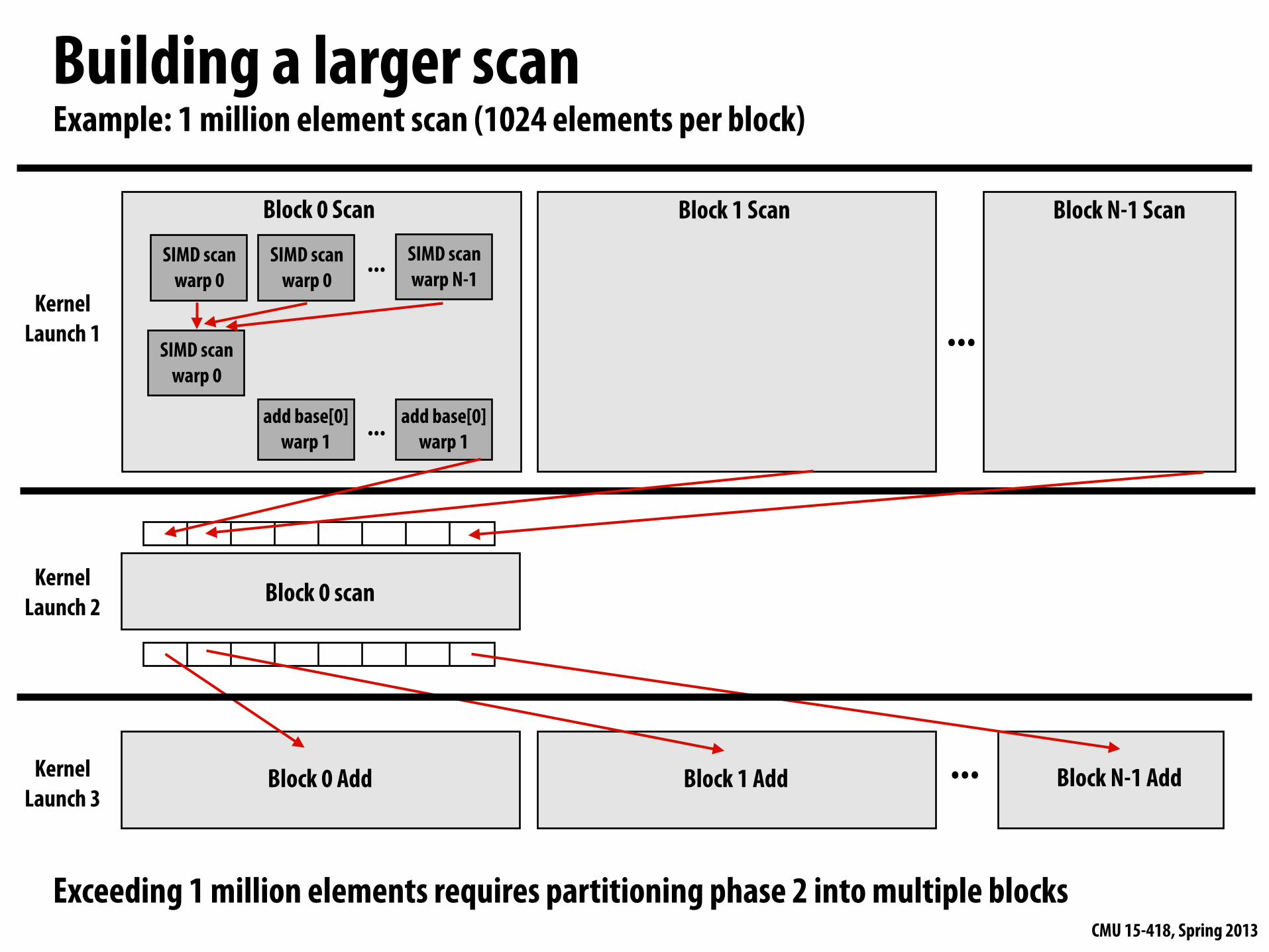
Building a larger scan
SIMD scanwarp 0
Example: 1 million element scan (1024 elements per block)
Block 0 Scan
add base[0]warp 1
...SIMD scanwarp 0
SIMD scanwarp N-1
SIMD scanwarp 0
add base[0]warp 1...
Block 1 Scan Block N-1 Scan
...
Block 0 scan
Block 0 Add Block 1 Add ... Block N-1 Add
Exceeding 1 million elements requires partitioning phase 2 into multiple blocks
Kernel Launch 1
Kernel Launch 2
Kernel Launch 3
CMU 15-418, Spring 2013
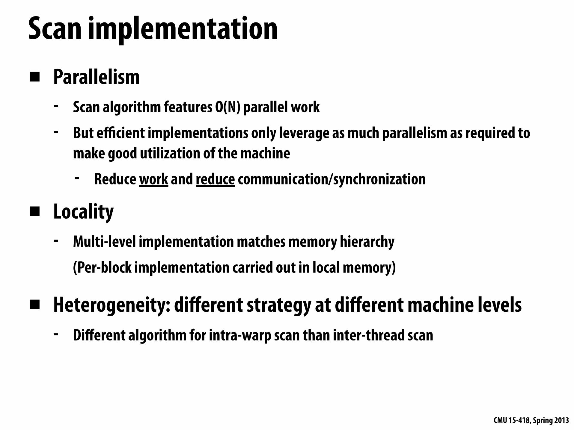
Scan implementation▪ Parallelism
- Scan algorithm features O(N) parallel work- But efficient implementations only leverage as much parallelism as required to
make good utilization of the machine- Reduce work and reduce communication/synchronization
▪ Locality- Multi-level implementation matches memory hierarchy
(Per-block implementation carried out in local memory)
▪ Heterogeneity: different strategy at different machine levels- Different algorithm for intra-warp scan than inter-thread scan
CMU 15-418, Spring 2013
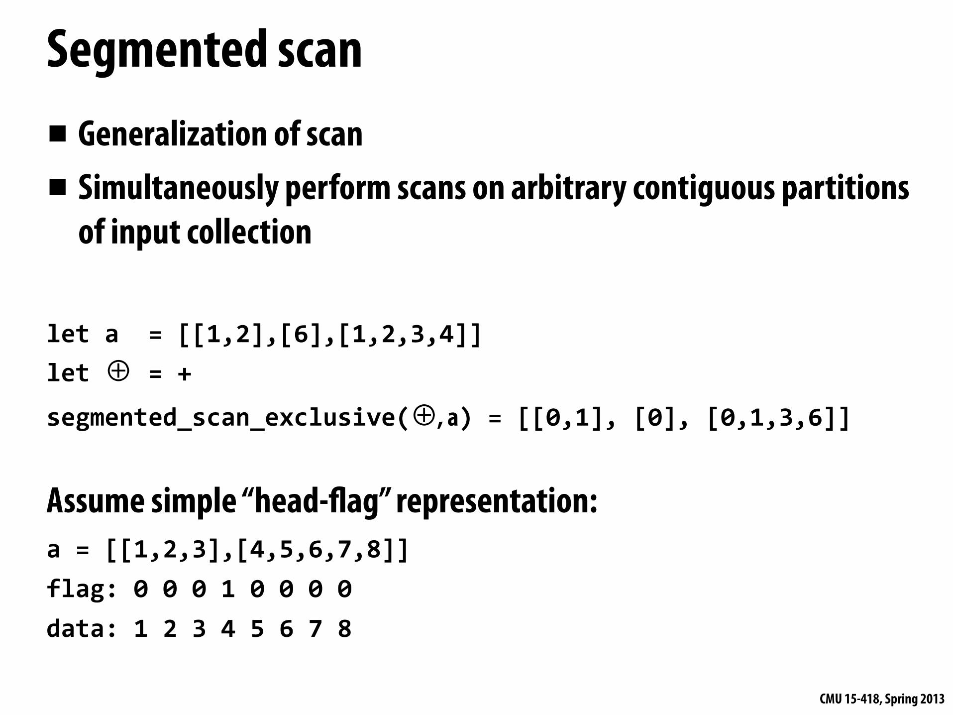
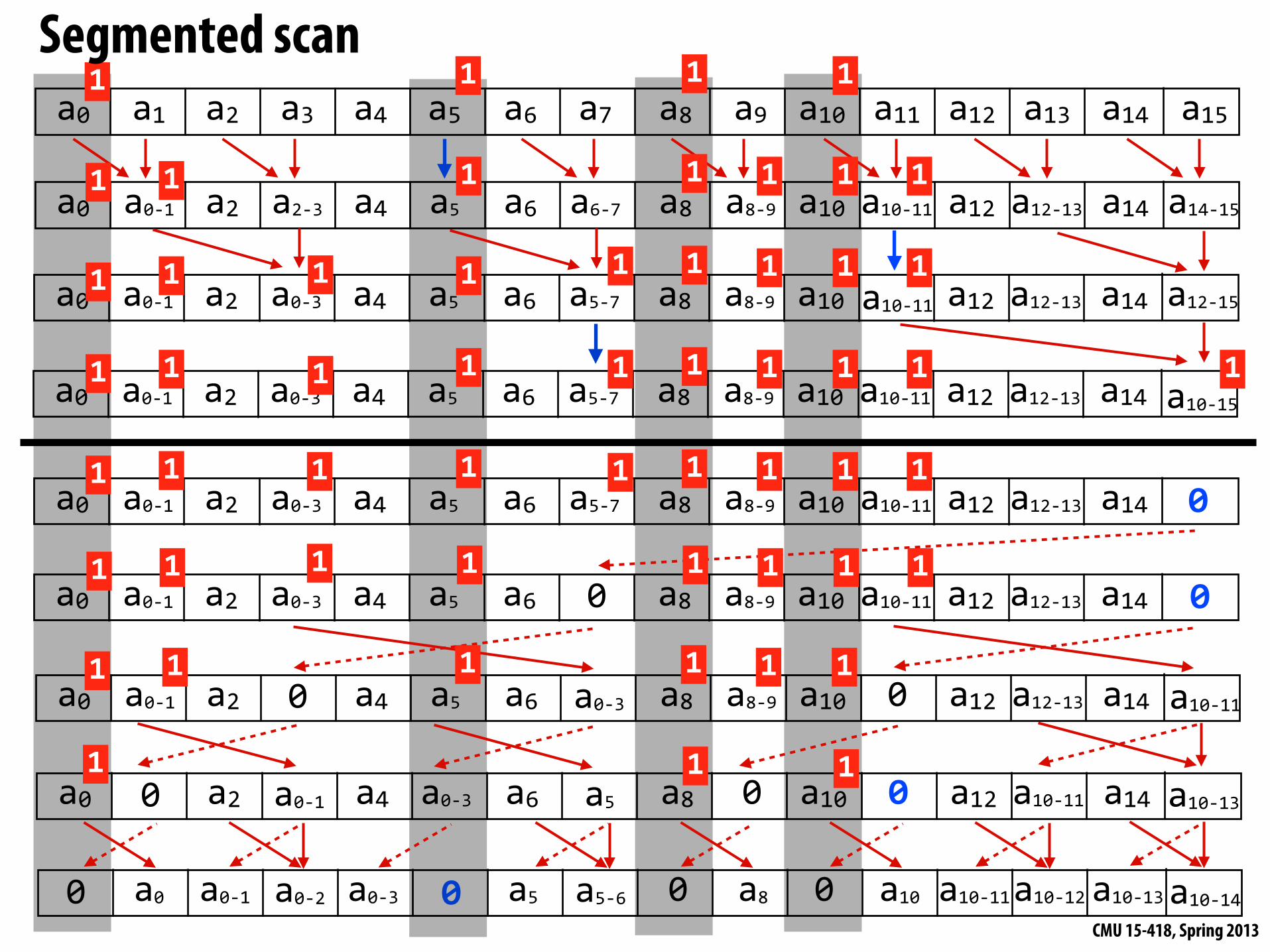
Segmented scan▪ Generalization of scan▪ Simultaneously perform scans on arbitrary contiguous partitions
of input collection
let a = [[1,2],[6],[1,2,3,4]]let ⊕ = +
segmented_scan_exclusive(⊕, a) = [[0,1], [0], [0,1,3,6]]
Assume simple “head-"ag” representation:a = [[1,2,3],[4,5,6,7,8]]flag: 0 0 0 1 0 0 0 0data: 1 2 3 4 5 6 7 8
CMU 15-418, Spring 2013
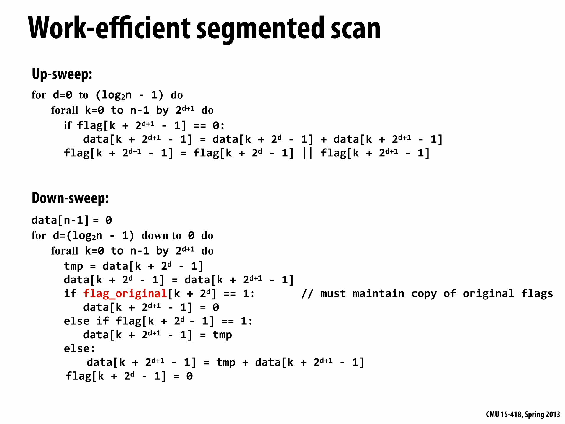
Work-efficient segmented scan
for d=0 to (log2n -‐ 1) do forall k=0 to n-‐1 by 2d+1 do if flag[k + 2d+1 -‐ 1] == 0: data[k + 2d+1 -‐ 1] = data[k + 2d -‐ 1] + data[k + 2d+1 -‐ 1] flag[k + 2d+1 -‐ 1] = flag[k + 2d -‐ 1] || flag[k + 2d+1 -‐ 1]
data[n-‐1] = 0for d=(log2n -‐ 1) down to 0 do forall k=0 to n-‐1 by 2d+1 do tmp = data[k + 2d -‐ 1] data[k + 2d -‐ 1] = data[k + 2d+1 -‐ 1] if flag_original[k + 2d] == 1: // must maintain copy of original flags data[k + 2d+1 -‐ 1] = 0 else if flag[k + 2d -‐ 1] == 1: data[k + 2d+1 -‐ 1] = tmp else:
data[k + 2d+1 -‐ 1] = tmp + data[k + 2d+1 -‐ 1] flag[k + 2d -‐ 1] = 0
Down-sweep:
Up-sweep:
CMU 15-418, Spring 2013
a0 a1 a2 a3 a4 a5 a6 a7 a8 a9 a10 a11 a12 a13 a14 a15
a0 a0-‐1 a2 a2-‐3 a4 a5 a6 a6-‐7 a8 a8-‐9 a10 a10-‐11 a12 a12-‐13 a14 a14-‐15
a0 a0-‐1 a2 a0-‐3 a4 a5 a6 a5-‐7 a8 a8-‐9 a10 a10-‐11 a12 a12-‐13 a14 a12-‐15
a0 a0-‐1 a2 a0-‐3 a4 a5 a6 a5-‐7 a8 a8-‐9 a10 a10-‐11 a12 a12-‐13 a14 a10-‐15
a0 a0-‐1 a2 a0-‐3 a4 a5 a6 a5-‐7 a8 a8-‐9 a10 a10-‐11 a12 a12-‐13 a14 0
a0 a0-‐1 a2 a0-‐3 a4 a5 a6 0 a8 a8-‐9 a10 a10-‐11 a12 a12-‐13 a14 0
a0 a0-‐1 a2 0 a4 a5 a6 a0-‐3 a8 a8-‐9 a10 0 a12 a12-‐13 a14 a10-‐11
a0 0 a2 a0-‐1 a4 a0-‐3 a6 a5 a8 0 a10 0 a12 a10-‐11 a14 a10-‐13
a00 a0-‐1 a0-‐2 a0-‐3 0 a5 a5-‐6 0 a8 0 a10 a10-‐11a10-‐12 a10-‐13 a10-‐14
1 1
1 1
1 1
11
1
1
1
1
1
1
1
1
1
1
1
1
1
1
1 1111
1 1111
1 111
11
1
1
1
1
1
1
1
1
1
1
1
1
1
1
1
1
1
1
Segmented scan
CMU 15-418, Spring 2013
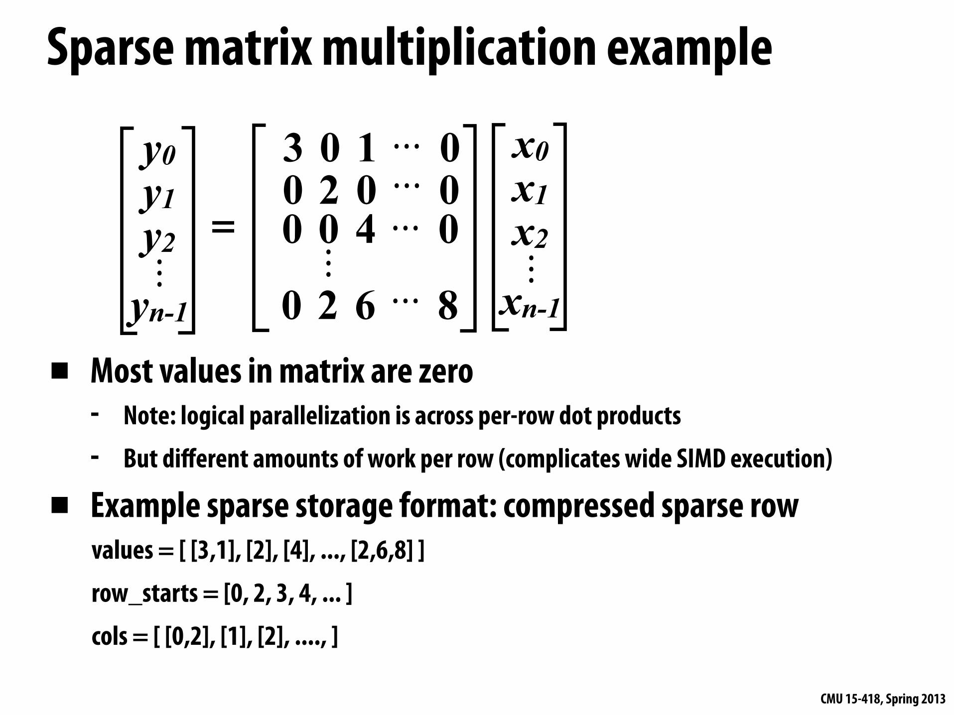
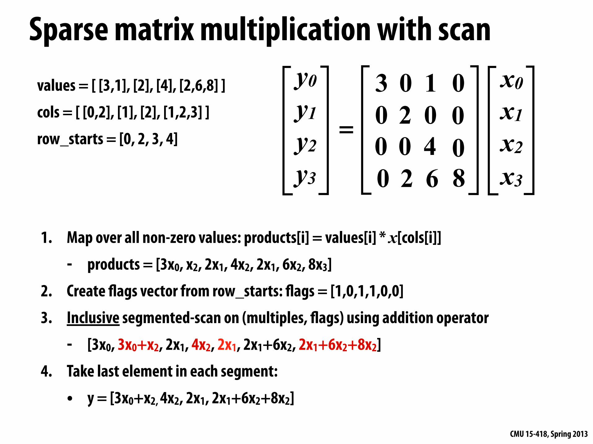
Sparse matrix multiplication example
=
x0 x1 x2
xn-1...
y0 y1 y2
yn-1...
3 0 0
1 0. . .
0 0. . . 2 0 0
0
4 0. . .
6 8. . . 2...
▪ Most values in matrix are zero- Note: logical parallelization is across per-row dot products- But different amounts of work per row (complicates wide SIMD execution)
▪ Example sparse storage format: compressed sparse rowvalues = [ [3,1], [2], [4], ..., [2,6,8] ]row_starts = [0, 2, 3, 4, ... ]cols = [ [0,2], [1], [2], ...., ]
CMU 15-418, Spring 2013
Sparse matrix multiplication with scan
1. Map over all non-zero values: products[i] = values[i] * x[cols[i]]
- products = [3x0, x2, 2x1, 4x2, 2x1, 6x2, 8x3]2. Create "ags vector from row_starts: "ags = [1,0,1,1,0,0]3. Inclusive segmented-scan on (multiples, "ags) using addition operator
- [3x0, 3x0+x2, 2x1, 4x2, 2x1, 2x1+6x2, 2x1+6x2+8x2]4. Take last element in each segment:
• y = [3x0+x2, 4x2, 2x1, 2x1+6x2+8x2]
=
x0 x1 x2 x3
y0 y1 y2 y3
3 0 0
1 0 2
0 0 0
4 6 8 2
0 0 0
values = [ [3,1], [2], [4], [2,6,8] ]cols = [ [0,2], [1], [2], [1,2,3] ]row_starts = [0, 2, 3, 4]
CMU 15-418, Spring 2013
Scan/segmented scan summary▪ Scan
- Parallel implementation of (intuitively sequential application)- Theory: parallelism linear in number of elements- Practice: exploit locality, use only as much parallelism as necessary to #ll the
machine- Great example of applying different strategies at different levels of the machine
▪ Segmented scan- Express computation and operate on irregular data structures (e.g., list of lists) in a
regular, data parallel way
CMU 15-418, Spring 2013
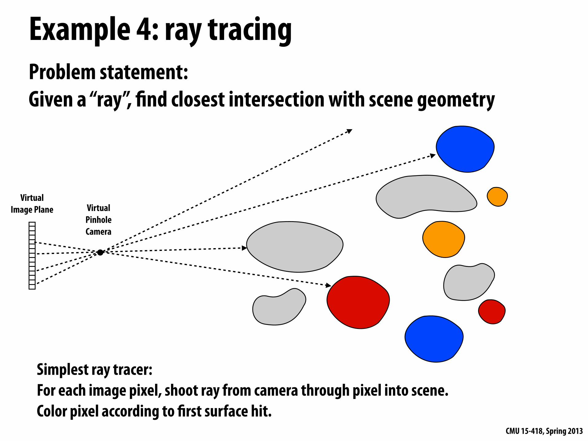
Example 4: ray tracingProblem statement:Given a “ray”, #nd closest intersection with scene geometry
VirtualPinhole Camera
VirtualImage Plane
Simplest ray tracer:For each image pixel, shoot ray from camera through pixel into scene.Color pixel according to #rst surface hit.
CMU 15-418, Spring 2013
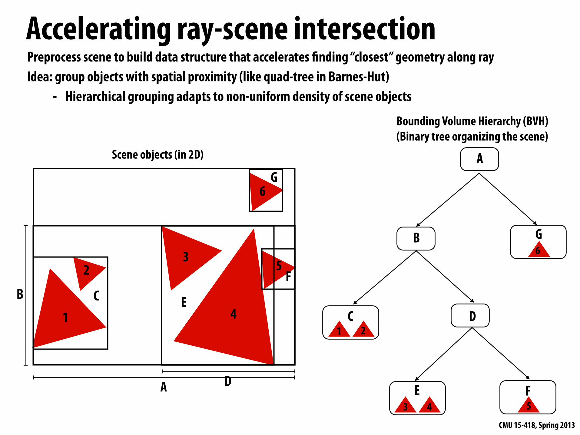
Accelerating ray-scene intersection Preprocess scene to build data structure that accelerates "nding “closest” geometry along rayIdea: group objects with spatial proximity (like quad-tree in Barnes-Hut)
- Hierarchical grouping adapts to non-uniform density of scene objects
Scene objects (in 2D)
1
2 3
4
5
C E
F
D
B
C D
E F
1 2
3 4 5
6
G6
A
A
G
B
Bounding Volume Hierarchy (BVH)(Binary tree organizing the scene)
CMU 15-418, Spring 2013
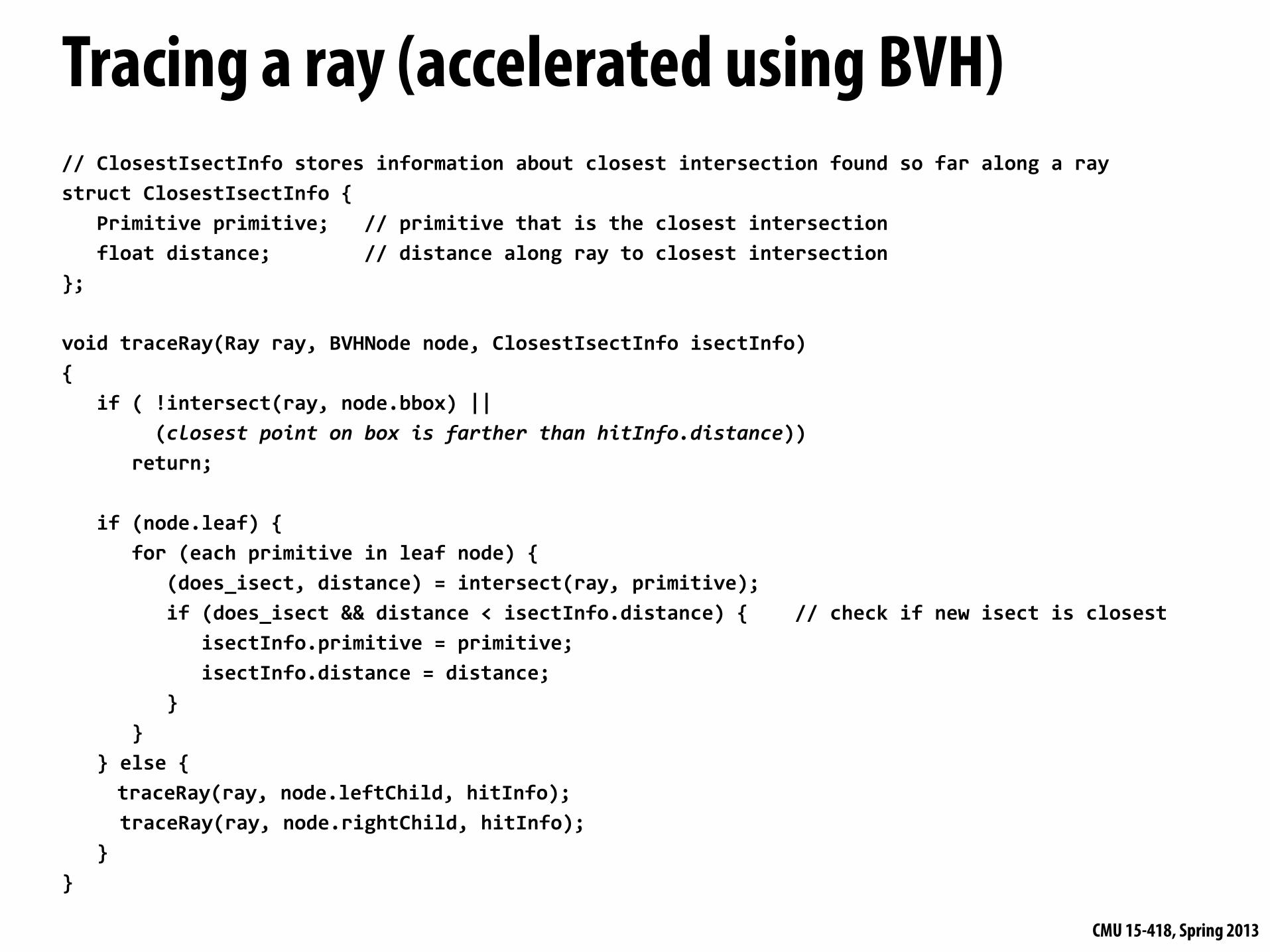
Tracing a ray (accelerated using BVH)// ClosestIsectInfo stores information about closest intersection found so far along a raystruct ClosestIsectInfo { Primitive primitive; // primitive that is the closest intersection float distance; // distance along ray to closest intersection};
void traceRay(Ray ray, BVHNode node, ClosestIsectInfo isectInfo){ if ( !intersect(ray, node.bbox) || (closest point on box is farther than hitInfo.distance)) return;
if (node.leaf) { for (each primitive in leaf node) { (does_isect, distance) = intersect(ray, primitive); if (does_isect && distance < isectInfo.distance) { // check if new isect is closest isectInfo.primitive = primitive; isectInfo.distance = distance; } } } else {
traceRay(ray, node.leftChild, hitInfo); traceRay(ray, node.rightChild, hitInfo); }}
CMU 15-418, Spring 2013
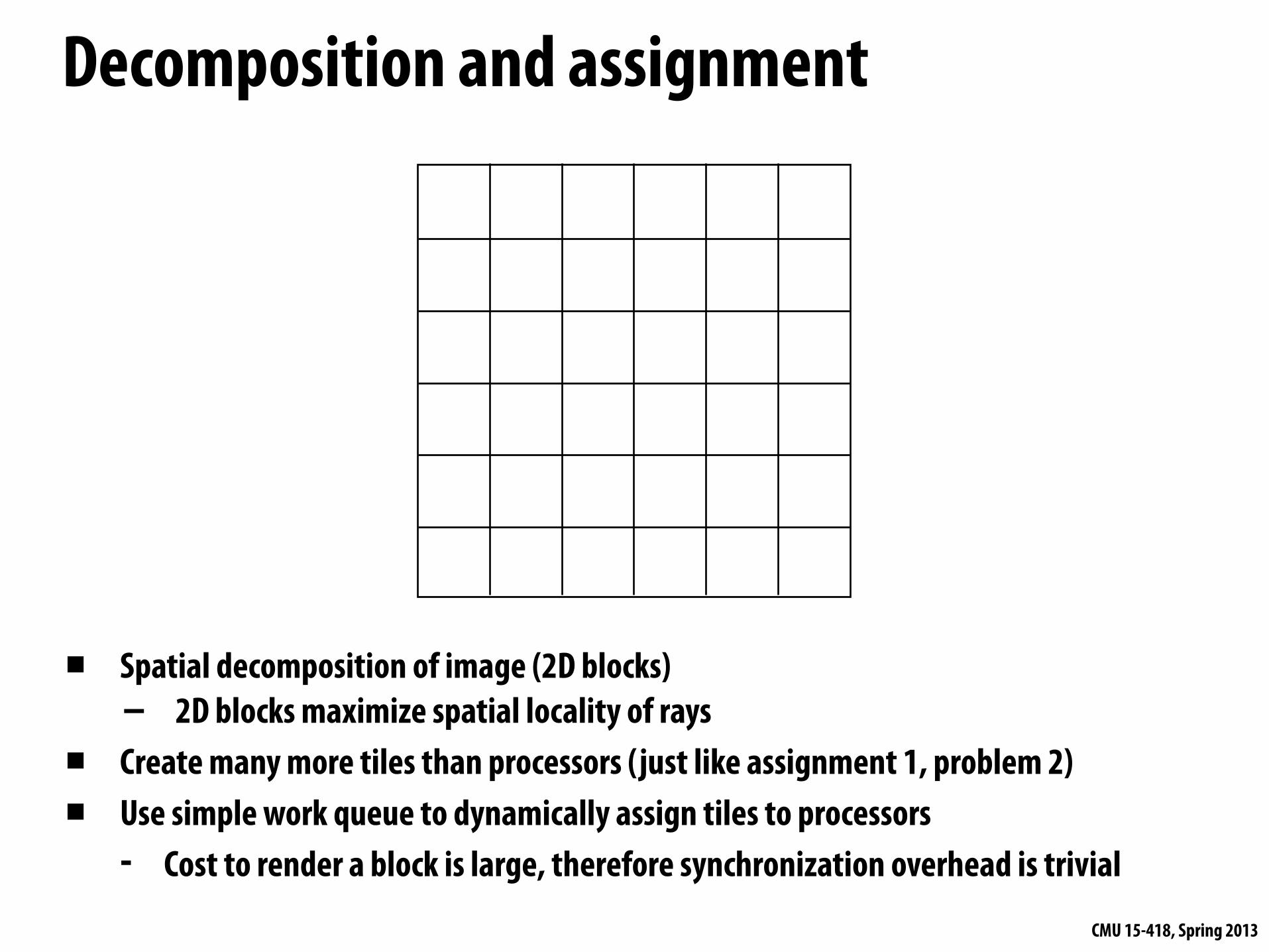
Decomposition and assignment
▪ Spatial decomposition of image (2D blocks)- 2D blocks maximize spatial locality of rays
▪ Create many more tiles than processors (just like assignment 1, problem 2)▪ Use simple work queue to dynamically assign tiles to processors
- Cost to render a block is large, therefore synchronization overhead is trivial
CMU 15-418, Spring 2013
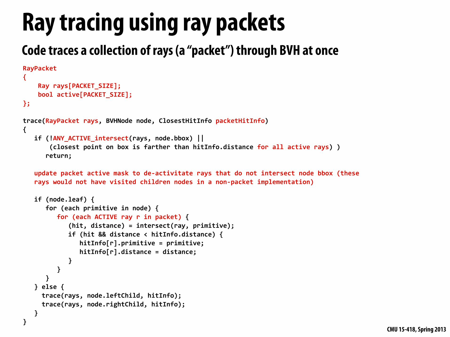
Ray tracing using ray packetsCode traces a collection of rays (a “packet”) through BVH at once RayPacket{ Ray rays[PACKET_SIZE]; bool active[PACKET_SIZE];};
trace(RayPacket rays, BVHNode node, ClosestHitInfo packetHitInfo){ if (!ANY_ACTIVE_intersect(rays, node.bbox) || (closest point on box is farther than hitInfo.distance for all active rays) ) return;
update packet active mask to de-‐activitate rays that do not intersect node bbox (these rays would not have visited children nodes in a non-‐packet implementation)
if (node.leaf) { for (each primitive in node) { for (each ACTIVE ray r in packet) { (hit, distance) = intersect(ray, primitive); if (hit && distance < hitInfo.distance) { hitInfo[r].primitive = primitive; hitInfo[r].distance = distance; } } } } else { trace(rays, node.leftChild, hitInfo); trace(rays, node.rightChild, hitInfo); }}
CMU 15-418, Spring 2013
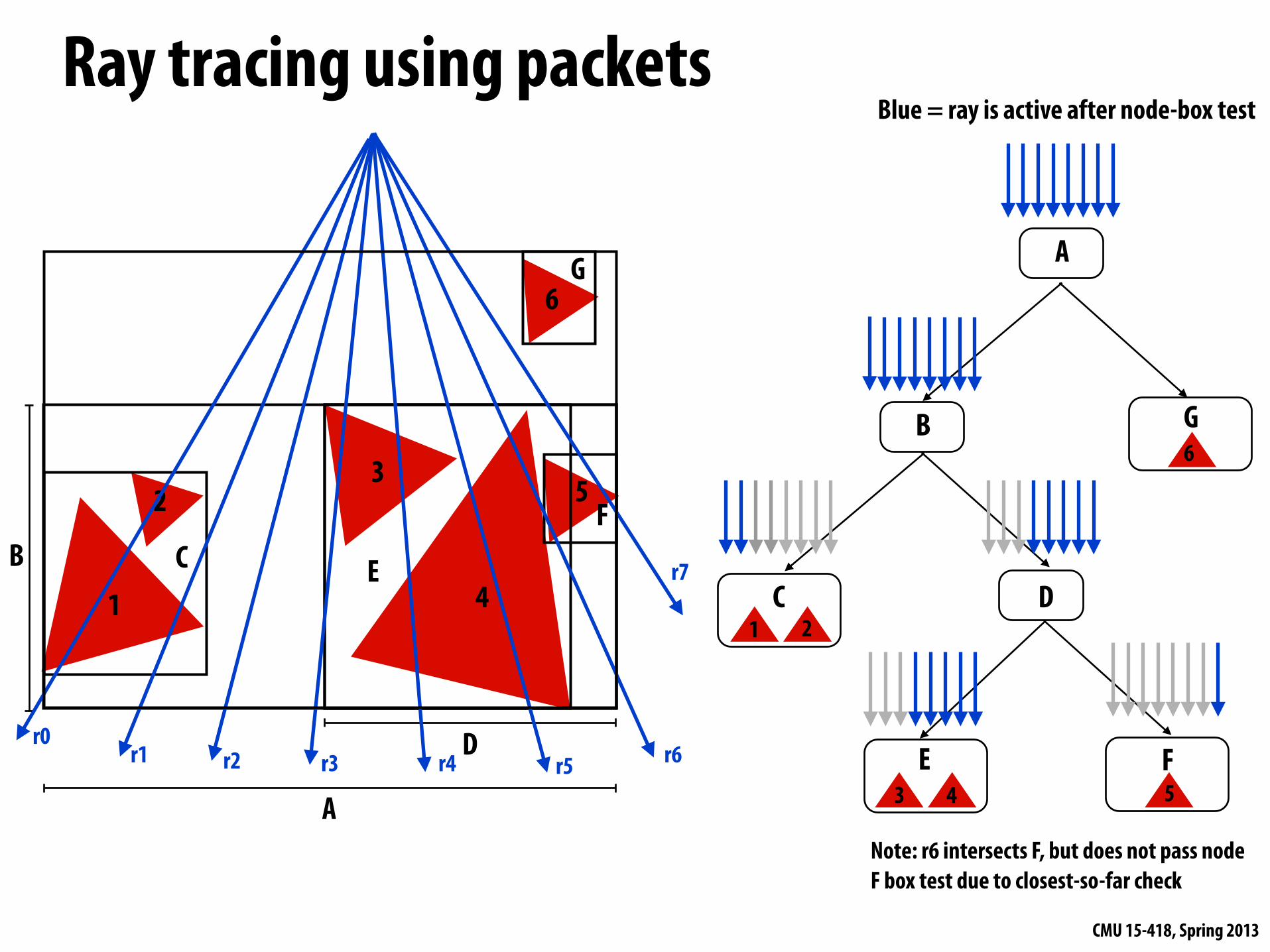
Ray tracing using packets
1
2 3
4
5
C E
F
D
B
B
C D
E F
1 2
3 4 5
6
G6
A
A
G
Blue = ray is active after node-box test
r0 r1 r2 r3 r4 r5 r6
r7
Note: r6 intersects F, but does not pass node F box test due to closest-so-far check
CMU 15-418, Spring 2013
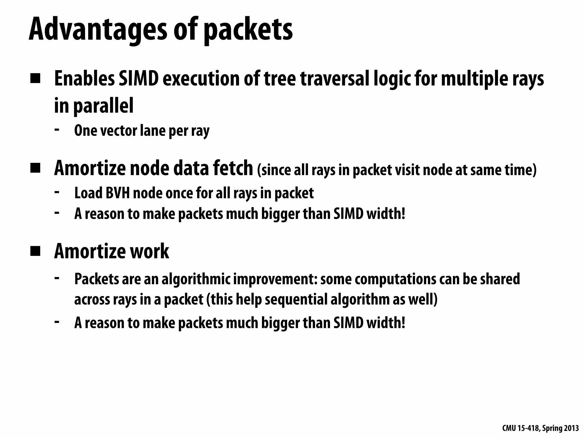
Advantages of packets▪ Enables SIMD execution of tree traversal logic for multiple rays
in parallel- One vector lane per ray
▪ Amortize node data fetch (since all rays in packet visit node at same time)- Load BVH node once for all rays in packet- A reason to make packets much bigger than SIMD width!
▪ Amortize work- Packets are an algorithmic improvement: some computations can be shared
across rays in a packet (this help sequential algorithm as well)- A reason to make packets much bigger than SIMD width!
CMU 15-418, Spring 2013
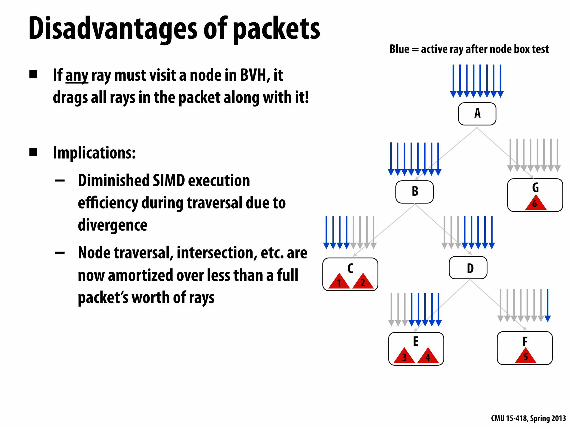
Disadvantages of packets
B
C D
E F
1 2
3 4 5
G6
A
Blue = active ray after node box test
▪ If any ray must visit a node in BVH, it drags all rays in the packet along with it!
▪ Implications:- Diminished SIMD execution
efficiency during traversal due to divergence
- Node traversal, intersection, etc. are now amortized over less than a full packet’s worth of rays
CMU 15-418, Spring 2013
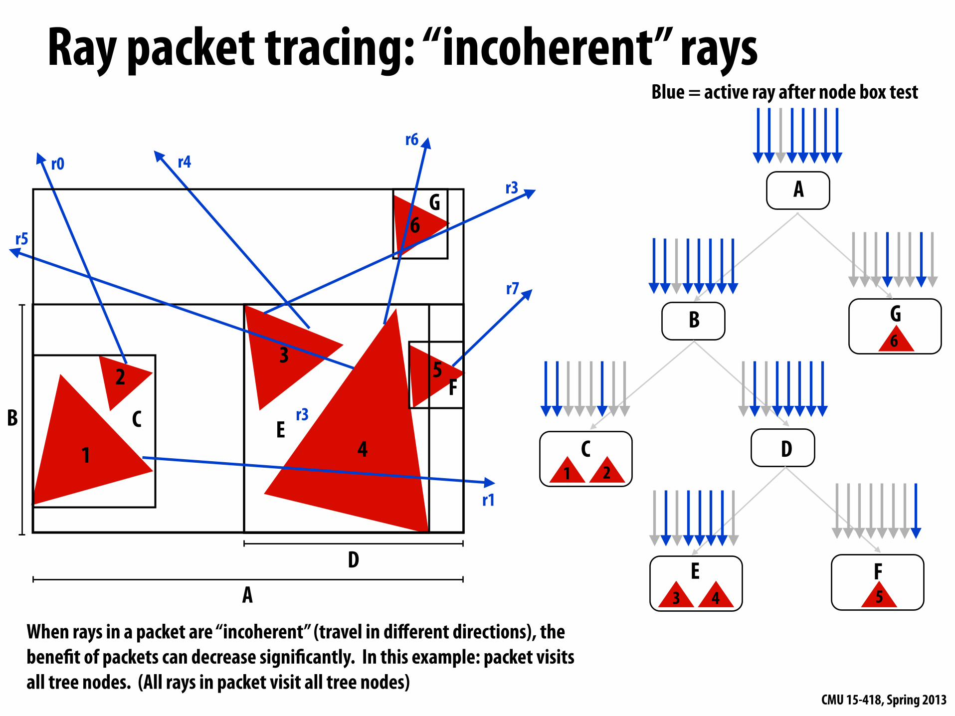
Ray packet tracing: “incoherent” rays
1
2 3
4
5
C E
F
D
B
B
C D
E F
1 2
3 4 5
6
G6
A
A
G
Blue = active ray after node box test
r0
r1
r3
r3
r4
r5
r6
r7
When rays in a packet are “incoherent” (travel in different directions), the bene#t of packets can decrease signi#cantly. In this example: packet visits all tree nodes. (All rays in packet visit all tree nodes)
CMU 15-418, Spring 2013
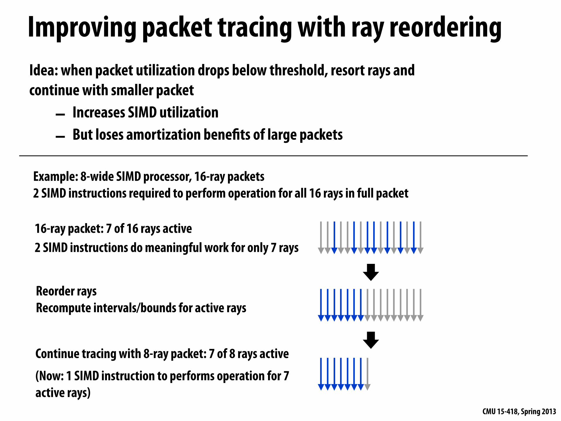
Improving packet tracing with ray reordering
16-ray packet: 7 of 16 rays active2 SIMD instructions do meaningful work for only 7 rays
Reorder raysRecompute intervals/bounds for active rays
Continue tracing with 8-ray packet: 7 of 8 rays active(Now: 1 SIMD instruction to performs operation for 7 active rays)
Example: 8-wide SIMD processor, 16-ray packets2 SIMD instructions required to perform operation for all 16 rays in full packet
Idea: when packet utilization drops below threshold, resort rays and continue with smaller packet- Increases SIMD utilization- But loses amortization bene#ts of large packets
CMU 15-418, Spring 2013
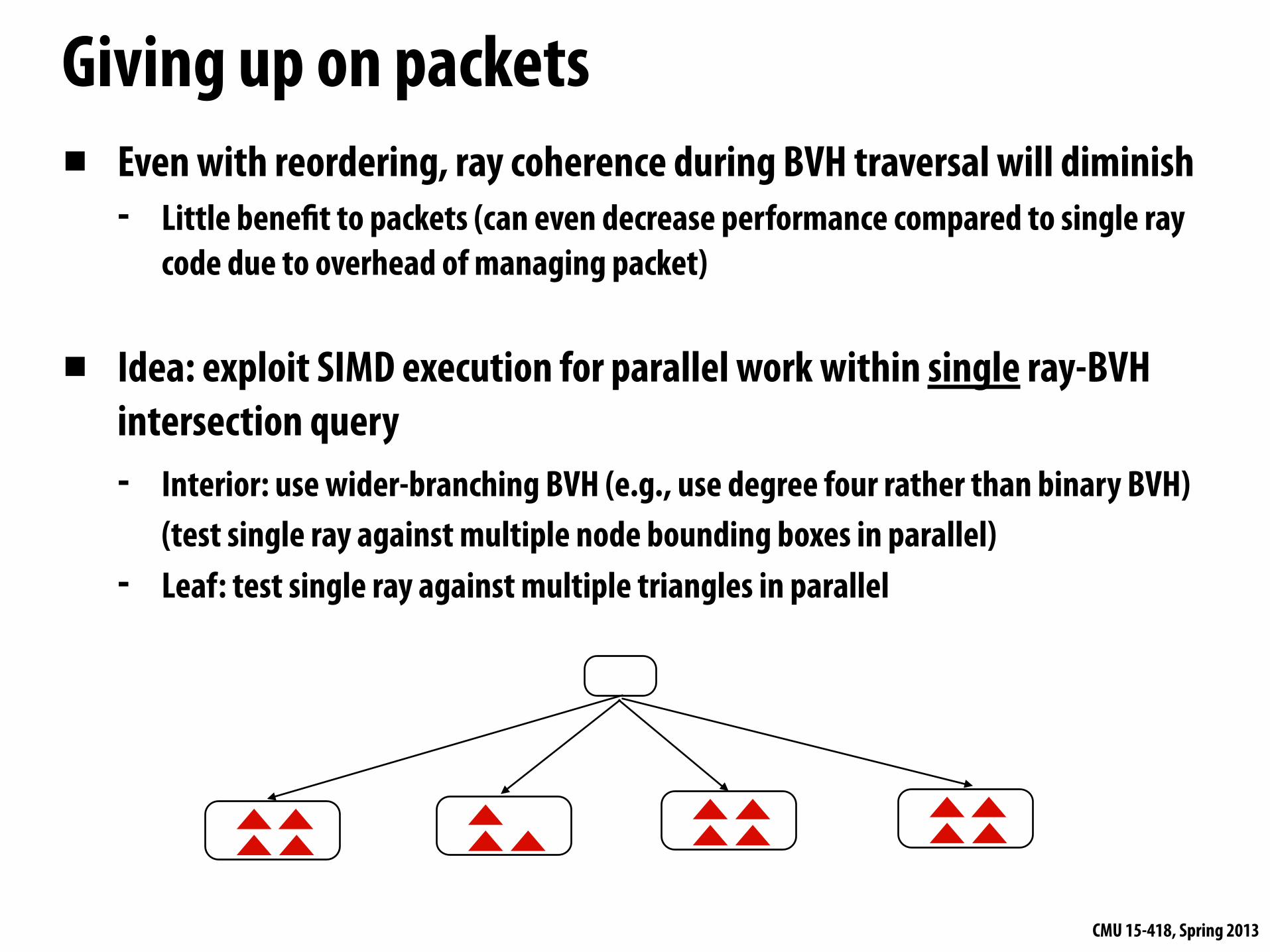
Giving up on packets▪ Even with reordering, ray coherence during BVH traversal will diminish
- Little bene#t to packets (can even decrease performance compared to single ray code due to overhead of managing packet)
▪ Idea: exploit SIMD execution for parallel work within single ray-BVH intersection query- Interior: use wider-branching BVH (e.g., use degree four rather than binary BVH)
(test single ray against multiple node bounding boxes in parallel)- Leaf: test single ray against multiple triangles in parallel
CMU 15-418, Spring 2013
Ray tracing best practices on multi-core CPU▪ Trivial assignment of screen regions to CPU cores
- Use work queue to dynamically assign regions of screen to cores(some regions may be more expensive than others)
▪ Effective use of SIMD execution is harder- Use large packets for higher levels of BVH
- Ray coherence always high at the top of the tree (visited by all rays)- Can switch to single ray (use SIMD for intra-ray parallelism) when packet utilization
drops below threshold- Can use dynamic reordering to postpone time of switch
- Reordering allows packets to provide bene!t deeper into tree
▪ Building a BVH in parallel is a tricky problem- Multiple threads must cooperate to build a shared structure- Not addressed here
CMU 15-418, Spring 2013
Summary▪ Today we looked at several different parallel programs
▪ Key questions:- What are the dependencies?- What synchronization is necessary? - How to balance the work?- How to exploit locality inherent in the problem?
▪ Trends- Only need enough parallelism to keep all processing elements busy (e.g., data-
parallel scan vs. simple multi-core scan)- Different parallelization strategies may be applicable under different
workloads (packets vs. no packets) or different locations in the machine (different implementations of scan internal and external to warp)
Top Related