


Languages
Pages
Legal

Particle Filter Example Approach for Lane Detection Filter at Work Random Particles Particle Weights Other Variants
Particle Filter1
Lecture 24
See Section 9.3.3 inReinhard Klette: Concise Computer Vision
Springer-Verlag, London, 2014
1See last slide for copyright information.1 / 33

Particle Filter Example Approach for Lane Detection Filter at Work Random Particles Particle Weights Other Variants
Agenda
1 Particle Filter
2 Example: Lane Border Detection
3 Approach for Lane Detection
4 Particle Filter at Work
5 Random Particles
6 Particle Weights and Condensation
7 Other Variants of Particle Filters
2 / 33

Particle Filter Example Approach for Lane Detection Filter at Work Random Particles Particle Weights Other Variants
Particles, Iterative Condensation, and Particle Weights
A particle represents a feature in a multi-dimensional space, theparticle space
Dimensions of this space may combine, e.g., locations, such as(x , y) in the image, or just coordinate x on a specified row in theimage, with descriptor values in a parameter vectora = (a1, a2, . . . , am) at a location; e.g. m + 2 dimensions for axesx , y , a1, . . . , am
A distribution of particles in particle space is transformed bycondensation into a new distribution taking weights of particlesinto account
3 / 33

Particle Filter Example Approach for Lane Detection Filter at Work Random Particles Particle Weights Other Variants
A 3D Particle Space
Iteration ta1
a2
x
Iteration t+1a1
a2
x
One spatial component x and two descriptor components a1 and a2
Condensation maps weighted particles from Iteration t to t + 1
Gray values indicate weights; weights change in iteration steps4 / 33

Particle Filter Example Approach for Lane Detection Filter at Work Random Particles Particle Weights Other Variants
Winning Particle
Particle filter can track parameter vectors over time or within aspace, based on evaluating consistency with a defined model
By evaluating the consistency of a particle with the model, weassign a weight (a non-negative real) to the particle
Condensation algorithm
For analyzing a cluster of weighted particles for identifying awinning particle
Many different strategies: typically, weights are recalculated initerations for the given cluster of weighted particles
Can also merge particles, change positions, or create new particles
Iteration stops: some kind of mean or local maxima is taken as awinning particle
5 / 33

Particle Filter Example Approach for Lane Detection Filter at Work Random Particles Particle Weights Other Variants
Agenda
1 Particle Filter
2 Example: Lane Border Detection
3 Approach for Lane Detection
4 Particle Filter at Work
5 Random Particles
6 Particle Weights and Condensation
7 Other Variants of Particle Filters
6 / 33

Particle Filter Example Approach for Lane Detection Filter at Work Random Particles Particle Weights Other Variants
Example: Lane Border Detection
A feature combines a left and a right point in the same image row(e.g. left and right lane border on the road)
Such a feature to be tracked in the the same image, say from oneimage row to the next, i.e. bottom-up
Translational movement of both contributing points to one featurecan (slightly) differ (i.e. their distance can change)
7 / 33

Particle Filter Example Approach for Lane Detection Filter at Work Random Particles Particle Weights Other Variants
Caption
Figure on slide before illustrates a possible chain of subprocessesfor lane border detection
Top, left to right:Input frameBird’s eye viewDetected vertical edges
Bottom, left to right:Row components of Euclidean distance transform (EDT), shown asabsolute valuesDetected center of lane and lane bordersLane borders projected back into the perspective view of therecorded frames
8 / 33

Particle Filter Example Approach for Lane Detection Filter at Work Random Particles Particle Weights Other Variants
With (Vague) Model About Movement
Features (each defined by keypoint and descriptor) to be trackedbut we have a general (“vague”) model about the movement ofthose features
Example: Tracking in the same image, row by row (bottom-up)
Image I
y
x
l rRow y
Row y-1
9 / 33
Particle Filter Example Approach for Lane Detection Filter at Work Random Particles Particle Weights Other Variants
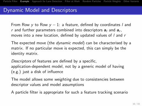
Dynamic Model and Descriptors
From Row y to Row y − 1: a feature, defined by coordinates l andr and further parameters combined into descriptors al and ar ,moves into a new location, defined by updated values of l and r
The expected move (the dynamic model) can be characterised by amatrix. If no particular move is expected, this can simply be theidentity matrix.
Descriptors of features are defined by a specific,application-dependent model, not by a generic model of having(e.g.) just a disk of influence
The model allows some weighting due to consistencies betweendescriptor values and model assumptions
A particle filter is appropriate for such a feature tracking scenario
10 / 33

Particle Filter Example Approach for Lane Detection Filter at Work Random Particles Particle Weights Other Variants
Agenda
1 Particle Filter
2 Example: Lane Border Detection
3 Approach for Lane Detection
4 Particle Filter at Work
5 Random Particles
6 Particle Weights and Condensation
7 Other Variants of Particle Filters
11 / 33

Particle Filter Example Approach for Lane Detection Filter at Work Random Particles Particle Weights Other Variants
Lane Borders
Task: Detection of lanes of a road in video data recorded in adriving ego-vehicle; brief outline of (a possible) general workflow:
1 Map recorded video frames into a bird’s-eye view
2 Detect vertical edges in bird’s-eye view, remove edge-artifacts
3 Perform Euclidean distance transform (EDT) for calculatingminimum distances between pixel locations p = (x , y) tothose edge pixels
[Use signed row components x − xedge of calculated distances√(x − xedge)2 + (y − yedge)2 for identifying centers of lanes at
places where signs are changing, and distance values about half of
the expected lane width]
4 Apply a particle filter for propagating detected lane borderpixels bottom-up, row by row, such that we have the mostlikely pixels as lane border pixels again in the next row
12 / 33

Particle Filter Example Approach for Lane Detection Filter at Work Random Particles Particle Weights Other Variants
Generating a Bird’s-Eye View
Step 1 on Slide 12 can be done by
1 inverse perspective mapping using the calibration data for theused camera (comment: more work-intensive; requirescalibration) or
2 simply by marking four pixels in the image, supposed to becorners of a rectangle in the plane of the road (thus appearingas a trapezoid in the perspective image), and by applying ahomography which maps those marked four points into arectangle, and at the same time the perspective view into abird’s-eye view
13 / 33

Particle Filter Example Approach for Lane Detection Filter at Work Random Particles Particle Weights Other Variants
Used Model
x
y
x
yl rc
α α h
l r
Left border Right border
β γ
Model visualization for the perspective image: Center point cdefines fixed height h angle α which identifies left and right laneborder points at l and r
Bird’s-view image: Model parameters defined for this view; atdetected points l and r , we have tangent angles β and γ to the leftand right border, detected as dominantly-vertical edges
14 / 33
Particle Filter Example Approach for Lane Detection Filter at Work Random Particles Particle Weights Other Variants
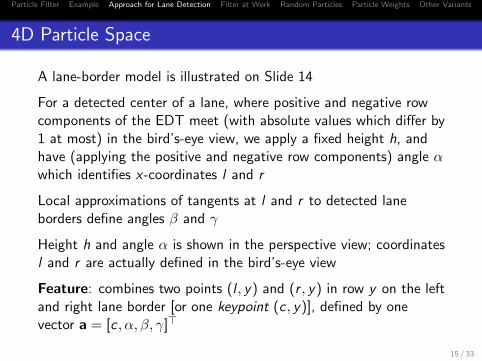
4D Particle Space
A lane-border model is illustrated on Slide 14
For a detected center of a lane, where positive and negative rowcomponents of the EDT meet (with absolute values which differ by1 at most) in the bird’s-eye view, we apply a fixed height h, andhave (applying the positive and negative row components) angle αwhich identifies x-coordinates l and r
Local approximations of tangents at l and r to detected laneborders define angles β and γ
Height h and angle α is shown in the perspective view; coordinatesl and r are actually defined in the bird’s-eye view
Feature: combines two points (l , y) and (r , y) in row y on the leftand right lane border [or one keypoint (c, y)], defined by onevector a = [c , α, β, γ]>
15 / 33

Particle Filter Example Approach for Lane Detection Filter at Work Random Particles Particle Weights Other Variants
Agenda
1 Particle Filter
2 Example: Lane Border Detection
3 Approach for Lane Detection
4 Particle Filter at Work
5 Random Particles
6 Particle Weights and Condensation
7 Other Variants of Particle Filters
16 / 33
Particle Filter Example Approach for Lane Detection Filter at Work Random Particles Particle Weights Other Variants
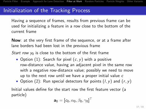
Initialization of the Tracking Process
Having a sequence of frames, results from previous frame can beused for initializing a feature in a row close to the bottom of thecurrent frame
Now: at the very first frame of the sequence, or at a frame afterlane borders had been lost in the previous frame
Start row y0 is close to the bottom of the first frame
• Option (1): Search for pixel (c , y) with a positiverow-distance value, having an adjacent pixel in the same rowwith a negative row-distance value; possibly we need to moveup to the next row until we have a proper initial value c
• Option (2): Run special detectors for points (l , y) and (r , y)
Initial values define for the start row the first feature vector (aparticle)
a0 = [c0, α0, β0, γ0]>
17 / 33

Particle Filter Example Approach for Lane Detection Filter at Work Random Particles Particle Weights Other Variants
Updating the Feature Vector of the Particle Filter
Track feature vector a = [c , α, β, γ]> (a particle) from start rowupward, up to a row which defines the upper limit for expectedlane borders (there are no lanes in the sky)
Row parameter y is calculated incrementally by applying a fixedincrement ∆, starting at y0 in the birds-eye image
Row at Step n is identified by yn = (y0 + n ·∆)
In the update process, a particle filter applies (in general) twoupdate models
18 / 33

Particle Filter Example Approach for Lane Detection Filter at Work Random Particles Particle Weights Other Variants
Two Update Models
The Dynamic Model
A dynamic model matrix A defines default motion of particles(here: in the image)
Let pn be the keypoint in Step n, expressed as a vector
Prediction value pn generated from pn−1 by pn = A · pn−1A general and simple choice: A = I (also used for our example)
The Observation Model
Determines a particle’s weight during resampling
19 / 33

Particle Filter Example Approach for Lane Detection Filter at Work Random Particles Particle Weights Other Variants
Observation Model for Given Example
Points (cn, yn) are assumed to have large absolute row-distancevalues
Let Ln and Rn be short digital line segments, centered at (ln, yn)and (rn, yn), representing the tangential lines at those two points inthe bird’s-eye view
It is assumed that these two line segments are formed by pixelswhich have absolute row-distance values (in EDT) close to 0
We assume that Ln and Rn are formed by an 8-path of length2k + 1, with points (ln, yn) or (rn, yn) at the middle position
20 / 33

Particle Filter Example Approach for Lane Detection Filter at Work Random Particles Particle Weights Other Variants
Agenda
1 Particle Filter
2 Example: Lane Border Detection
3 Approach for Lane Detection
4 Particle Filter at Work
5 Random Particles
6 Particle Weights and Condensation
7 Other Variants of Particle Filters
21 / 33

Particle Filter Example Approach for Lane Detection Filter at Work Random Particles Particle Weights Other Variants
Generation of Random Particles
In each step when going forward to the next row, we generateNpart > 0 particles randomly around the predicted parametervector (following the dynamic model) in mD particle space
For better results use a larger number of generated particles (e.g.Npart = 500)
The figure on Slide 4 illustrates 43 particles in a 3D particle space
The i th particle generated in Step n, for 1 ≤ i ≤ Npart
ain = [c in, αin, β
in, γ
in]>
22 / 33

Particle Filter Example Approach for Lane Detection Filter at Work Random Particles Particle Weights Other Variants
Particle Generation Using a Uniform Distribution
Apply a uniform distribution for generated particles in mD particlespace
For the discussed example:
For c we assume an interval [c − 10, c + 10], and we selectuniformly random values for the c-component in this interval
This process is independent from the other components of a vectorain
For the second component, we assume an interval (say) of[α− 0.1, α+ 0.1], for the third [β − 0.5, β + 0.5], and similar for γ
23 / 33

Particle Filter Example Approach for Lane Detection Filter at Work Random Particles Particle Weights Other Variants
Particle Generation Using a Gauss Distribution
We use a Gauss (or normal) distribution for the generated particlesin mD particle space
For the discussed example:
A zero-mean distribution produces values around the predictedvalue
For the individual components we assume a standard deviationσ > 0 such that we generate values about in the same intervals asspecified for the uniform distribution on the slide before
For example, we use σ = 10 for the c-component
24 / 33

Particle Filter Example Approach for Lane Detection Filter at Work Random Particles Particle Weights Other Variants
Agenda
1 Particle Filter
2 Example: Lane Border Detection
3 Approach for Lane Detection
4 Particle Filter at Work
5 Random Particles
6 Particle Weights and Condensation
7 Other Variants of Particle Filters
25 / 33

Particle Filter Example Approach for Lane Detection Filter at Work Random Particles Particle Weights Other Variants
Particle Weights
We define a weight for the ith particle ain
In the discussed example:
Left position equals
l in = c in − h · tan αin
Sum of absolute row-distance values dr (x , y) = |x − xedge |, asprovided by the EDT in the bird’s-eye view, along line segment L(assumed to be an 8-path of length 2k + 1) equals
S iL =
k∑j=−k
∣∣∣dr (l in + j · sin βin, yn + j · cos βin
)∣∣∣Calculate S i
R for the second line segment in an analogous way26 / 33

Particle Filter Example Approach for Lane Detection Filter at Work Random Particles Particle Weights Other Variants
Two Individual Weights
Obtain the weight
ωidist =
1
2σlσrπexp
(−
(S iL − µl)2
2σl−
(S iR − µr )2
2σr
)with respect to distance values on L and R, where µl , µr , σl , andσr are estimated constants (say, zero-mean µl = µr = 0 for theideal case) based on experiments for the given application
For the generated center point (c in, yn), the weight equals
ωicenter =
1
σc√
2πexp
−(∣∣∣ 1
dr (c in,yn)
∣∣∣− µc)22σc
where µc and σc are again estimated constants
27 / 33

Particle Filter Example Approach for Lane Detection Filter at Work Random Particles Particle Weights Other Variants
Total Weight
Total weight for the ith particle ain, at the beginning of theiterative condensation process, is given by
ωi = ωidist · ωi
center
These weights decide about the “influence” of the particles duringthe condensation process
A normalization of all the Npart weights is normally required beforeapplying one of the common condensation programs
There is a condensation procedure available in OpenCV: run for theselected numbers of iterations and use the specified winningparticle; this defines here the lane borders in the next image row;see CvConDensation
28 / 33
Particle Filter Example Approach for Lane Detection Filter at Work Random Particles Particle Weights Other Variants
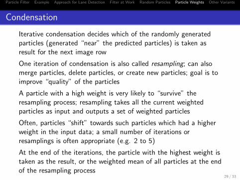
Condensation
Iterative condensation decides which of the randomly generatedparticles (generated “near” the predicted particles) is taken asresult for the next image row
One iteration of condensation is also called resampling; can alsomerge particles, delete particles, or create new particles; goal is toimprove “quality” of the particles
A particle with a high weight is very likely to “survive” theresampling process; resampling takes all the current weightedparticles as input and outputs a set of weighted particles
Often, particles “shift” towards such particles which had a higherweight in the input data; a small number of iterations orresamplings is often appropriate (e.g. 2 to 5)
At the end of the iterations, the particle with the highest weight istaken as the result, or the weighted mean of all particles at the endof the resampling process
29 / 33

Particle Filter Example Approach for Lane Detection Filter at Work Random Particles Particle Weights Other Variants
Agenda
1 Particle Filter
2 Example: Lane Border Detection
3 Approach for Lane Detection
4 Particle Filter at Work
5 Random Particles
6 Particle Weights and Condensation
7 Other Variants of Particle Filters
30 / 33
Particle Filter Example Approach for Lane Detection Filter at Work Random Particles Particle Weights Other Variants
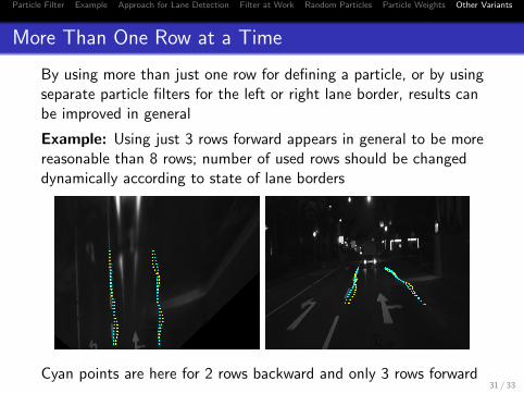
More Than One Row at a Time
By using more than just one row for defining a particle, or by usingseparate particle filters for the left or right lane border, results canbe improved in general
Example: Using just 3 rows forward appears in general to be morereasonable than 8 rows; number of used rows should be changeddynamically according to state of lane borders
Cyan points are here for 2 rows backward and only 3 rows forward31 / 33
Particle Filter Example Approach for Lane Detection Filter at Work Random Particles Particle Weights Other Variants
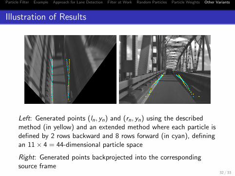
Illustration of Results
Left: Generated points (ln, yn) and (rn, yn) using the describedmethod (in yellow) and an extended method where each particle isdefined by 2 rows backward and 8 rows forward (in cyan), definingan 11× 4 = 44-dimensional particle space
Right: Generated points backprojected into the correspondingsource frame
32 / 33
Particle Filter Example Approach for Lane Detection Filter at Work Random Particles Particle Weights Other Variants
Copyright Information
This slide show was prepared by Reinhard Klettewith kind permission from Springer Science+Business Media B.V.
The slide show can be used freely for presentations.However, all the material is copyrighted.
R. Klette. Concise Computer Vision.c©Springer-Verlag, London, 2014.
In case of citation: just cite the book, that’s fine.
33 / 33
Top Related