


Languages
Pages
Legal


Lecture 14:Introduction to Logistic Regression
BMTRY 701Biostatistical Methods II

Binary outcomes
Linear regression is appropriate for continuous outcomes
in biomedical research, our outcomes are more commonly of different forms
Binary is probably the most prevalent• disease versus not disease• cured versus not cured• progressed versus not progressed• dead versus alive

Example: Prostate Cancer
PROSTATE CANCER DATA SETSIZE: 380 observations, 9 variables SOURCE: Hosmer and Lemeshow (2000) Applied Logistic egression: 2nd Edn.
1 Identification Code 1 – 380 ID 2 Tumor Penetration of 0 = No Penetration, CAPSULE Prostatic Capsule 1 = Penetration 3 Age Years AGE 4 Race 1= White, 2 = Black RACE 5 Results of Digital Rectal Exam 1 = No Nodule DPROS
2 = Unilobar Nodule (Left) 3 = Unilobar Nodule (Right) 4 = Bilobar Nodule
6 Detection of Capsular 1 = No, 2 = Yes DCAPS Involvement in Rectal Exam 7 Prostatic Specific Antigen Value mg/ml PSA 8 Tumor Volume from Ultrasound cm3 VOL 9 Total Gleason Score 0 - 10 GLEASON

What factors are related to capsular penetration?
The prostate capsule is the membrane the surrounds the prostate gland
As prostate cancer advances, the disease may extend into the capsule (extraprostatic extension) or beyond (extracapsular extension) and into the seminal vesicles.
Capsular penetration is a poor prognostic indicator, which accounts for a reduced survival expectancy and a higher progression rate following radical prostatectomy.
Let’s start with PSA and Gleason score Both are well-known factors related to disease severity What does a linear regression of capsular penetration on
PSA and Gleason mean?
ii eGSPSAY 2`0

PSA
PSA is the abbreviation for prostate-specific antigen which is an enzyme produced in the epithelial cells of both benign and malignant tissue of the prostate gland.
The enzyme keeps ejaculatory fluid from congealing after it has been expelled from the body.
Prostate-specific antigen is used as a tumor marker to determine the presence of prostate cancer because a greater prostatic volume, associated with prostate cancer, produces larger amount of prostate-specific antigen.
http://www.prostate-cancer.com/

Gleason Score
The prostate cancer Gleason Score is the sum of the two Gleason grades.
After a prostate biopsy, a pathologist examines the samples of prostate cancer cells to see how the patterns, sizes, and shapes are different from healthy prostate cells.
Cancerous cells that appear similar from healthy prostate are called well-differentiated while cancerous cells that appear very different from healthy prostate cells are called poorly-differentiated.
The pathologist assigns one Gleason grade to the most common pattern of prostate cancer cells and then assigns a second Gleason grade to the second-most common pattern of prostate cancer cells.
These two Gleason grades indicate prostate cancer’s aggresiveness, which indicates how quickly prostate cancer may extend out of the prostate gland.
Gleason score = Gleason 1 + Gleason 2
http://www.prostate-cancer.com/

What is Y?
Y is a binary outcome variable Observed data:
• Yi = 1 if patient if patient had capsular involvement
• Yi = 0 if patient did not have capsular involvement
But think about the ‘binomial distribution’ The parameter we are modeling is a probability, p We’d like to be able to find a model that relates the
probability of capsular involvement to covariates
ii eGSPSAYP 2`0)1(
For a one-unit increase in GS, we expect the probability of capsularpenetration to increase by β2.
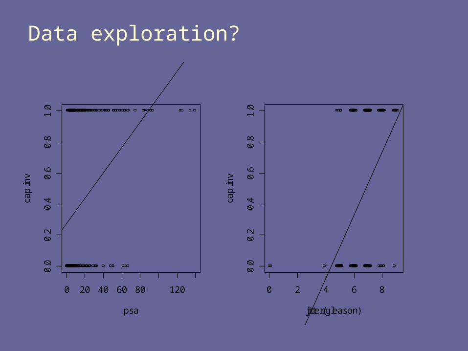
Data exploration?
0 20 40 60 80 120
0.0
0.2
0.4
0.6
0.8
1.0
psa
cap
.inv
0 2 4 6 8
0.0
0.2
0.4
0.6
0.8
1.0
jitter(gleason)
cap
.inv

What are the problems?
The interpretation does not make sense for a few reasons
You cannot have P(Y=1) values below 0 or 1 What about the behavior of residuals?
• normal? • constant variance?

Yikes!
0 20 40 60 80 120
-0.5
0.0
0.5
psa
reg
psa
$re
sid
ua
ls
0 2 4 6 8
-1.0
-0.5
0.0
0.5
jitter(gleason)
(re
gg
s$re
sid
ua
ls)
Why do they have these strange patterns?
(Based on simple linear regressions)

Properties of the residuals (with linear regression)
Nonnormal error terms• Each error term can only take one of two values:
Nonconstant error variance: the variance depends on X:
0
1 1
10
10
iii
iii
yifxe
yifxe
)1)((
)1(
)1()ˆ(
10102
2
ii xx
pp
pppVar

Clearly, that does not work!
A few things to consider We’d like to model the ‘probability’ of the event
occuring Y=1 or 0, but we can conceptualize values in
between as probabilities We cannot allow probabilities greater than 1 or
less than 0

“Link” functions: P(Y=1)
Logit link:
Probit link:
Complementary log-log:
)1(1
)1(log))1((logit
YP
YPYP
))1(())1(( 1 YPYPprobit
))]1(1log(log[))1(log(log YPYPc
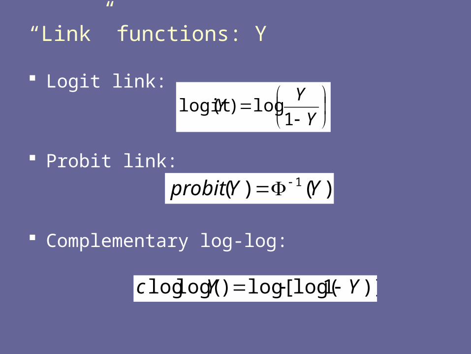
“Link” functions: Y
Logit link:
Probit link:
Complementary log-log:
Y
YY
1log)(logit
)()( 1 YYprobit
)]1log(log[)log(log YYc
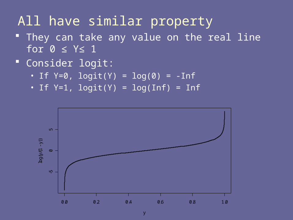
All have similar property They can take any value on the real line for 0 ≤ Y≤ 1 Consider logit:
• If Y=0, logit(Y) = log(0) = -Inf• If Y=1, logit(Y) = log(Inf) = Inf
0.0 0.2 0.4 0.6 0.8 1.0
-50
5
y
log
(y/(
1 -
y))

All three together
0.0 0.2 0.4 0.6 0.8 1.0
-4-2
02
4
y
link
fun
ctio
n
LogitProbitCLogLog

All three together
-4 -2 0 2 4
0.0
0.2
0.4
0.6
0.8
1.0
link function
y
LogitProbitCLogLog
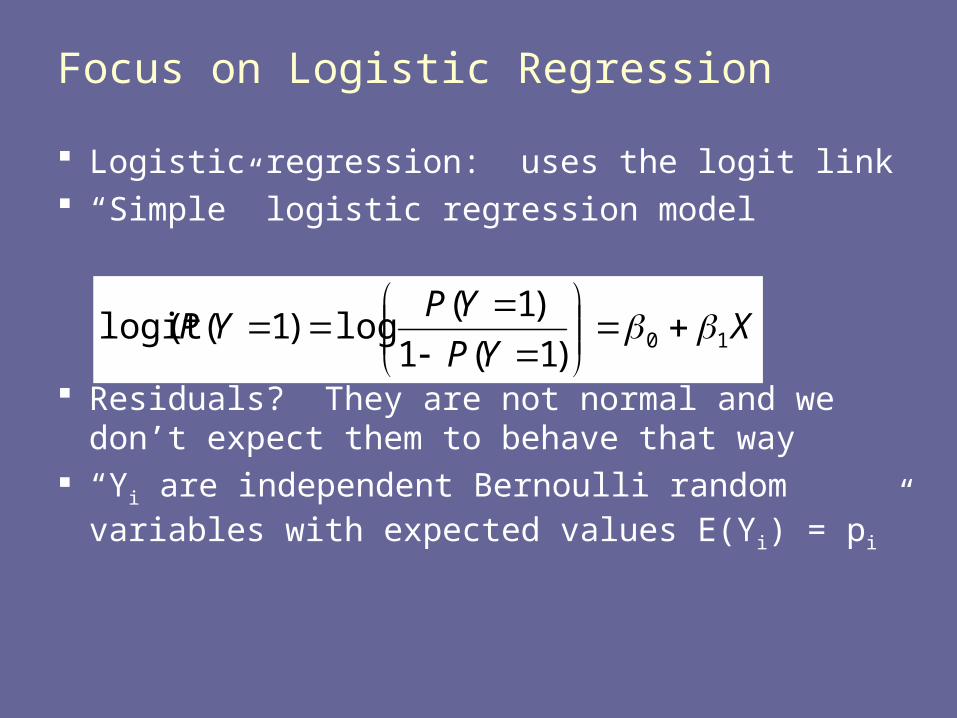
Focus on Logistic Regression
Logistic regression: uses the logit link “Simple” logistic regression model
Residuals? They are not normal and we don’t expect them to behave that way
“Yi are independent Bernoulli random variables with expected values E(Yi) = pi”
XYP
YPYP 10)1(1
)1(log)1((logit

E(Yi)
What is E(Yi) ?
• Let pi = P(Y=1)
• Then E(Yi) = 1*pi + 0*(1-pi) = pi
• Hence E(Yi) = P(Y=1) = pi
That will be our notation
Now, solve for pi:
Xp
pp
i
ii 101
log)(logit

pi
X)βexp( β1X)βexp( β
p10
10i
)exp())exp(1(
)exp()exp(
)exp()exp(
)exp()1(
)exp(1
1log
1010
1010
1010
10
10
10
XXp
XXpp
XpXp
Xpp
Xp
p
Xp
p
i
ii
ii
ii
i
i
i
i
Hence, the following are equivalent:
)Xβexp(β1
)Xβexp(βp
i10
i10i
ii Xp 10)(logit

Fitted values: two types
Linear predictor:
Fitted probability:
)Xβ̂β̂exp(1
)Xβ̂β̂exp(p̂
i10
i10i
ii Xp 10ˆˆ)(logit
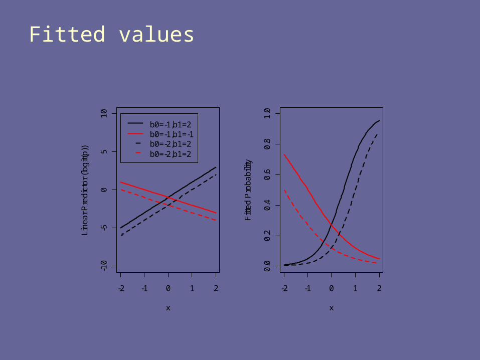
Fitted values
-2 -1 0 1 2
-10
-50
51
0
x
Lin
ea
r P
red
icto
r (l
og
it(p
))
b0=-1,b1=2b0=-1,b1=-1b0=-2,b1=2b0=-2,b1=2
-2 -1 0 1 2
0.0
0.2
0.4
0.6
0.8
1.0
x
Fitt
ed
Pro
ba
bili
ty

Prostate Cancer Example
Logistic regression of capsular penetration on PSA and Gleason Score
Notice that we don’t include the error term Implied assumption that the data (i.e. Y) is
binary (Bernoulli)
GSPSAp
p
i
i2`01
log
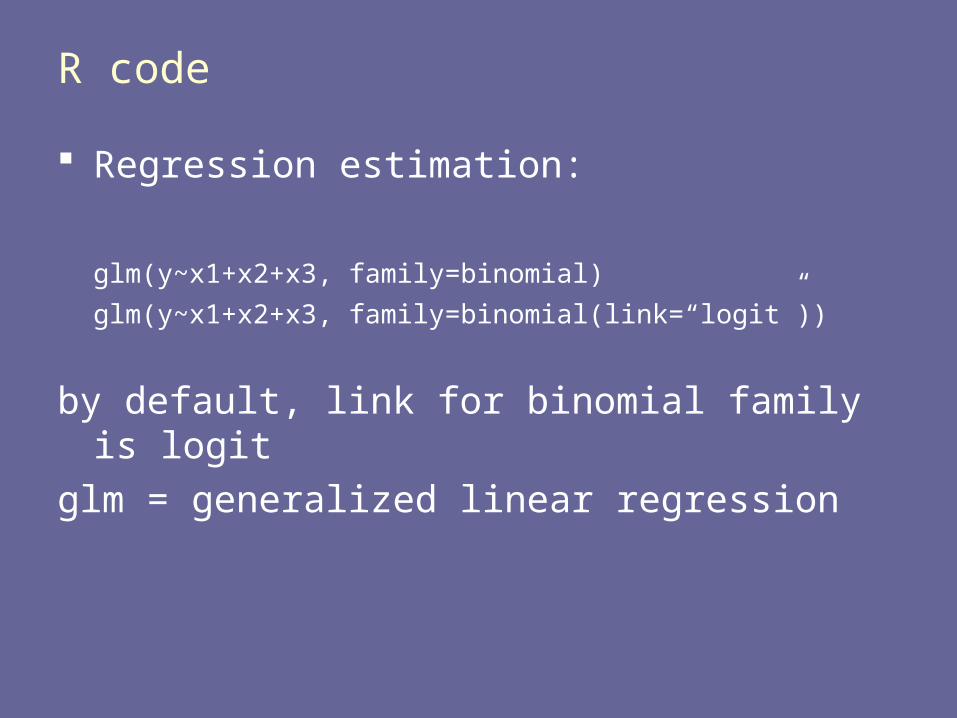
R code
Regression estimation:
glm(y~x1+x2+x3, family=binomial)
glm(y~x1+x2+x3, family=binomial(link=“logit”))
by default, link for binomial family is logit
glm = generalized linear regression
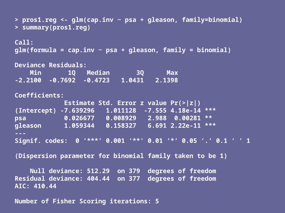
> pros1.reg <- glm(cap.inv ~ psa + gleason, family=binomial)> summary(pros1.reg)
Call:glm(formula = cap.inv ~ psa + gleason, family = binomial)
Deviance Residuals: Min 1Q Median 3Q Max -2.2100 -0.7692 -0.4723 1.0431 2.1398
Coefficients: Estimate Std. Error z value Pr(>|z|) (Intercept) -7.639296 1.011128 -7.555 4.18e-14 ***psa 0.026677 0.008929 2.988 0.00281 ** gleason 1.059344 0.158327 6.691 2.22e-11 ***---Signif. codes: 0 ‘***’ 0.001 ‘**’ 0.01 ‘*’ 0.05 ‘.’ 0.1 ‘ ’ 1
(Dispersion parameter for binomial family taken to be 1)
Null deviance: 512.29 on 379 degrees of freedomResidual deviance: 404.44 on 377 degrees of freedomAIC: 410.44
Number of Fisher Scoring iterations: 5

Interpreting the output
Beta coefficients What do they mean?
• log-odds ratios• example: comparing two men with Gleason scores that are one
unit different, the log odds ratio for capsular penetration is 1.06.
We usually exponentiate them:• exp(B2) = exp(1.06) = 2.88
• the odds of capsular penetration for a man with Gleason score of 7 is 2.88 times that of a man with Gleason score of 6
• The odds ratio for a 1 unit difference in Gleason score is 2.88
You also need to interpret them as ‘adjusting for PSA’

Inferences: Confidence intervals
Similar to that for linear regression But, not exactly the same
• The betas do NOT have a t distribution• But, asymptotically, they are normally distributed
Implications? we always use quantiles of the NORMAL distribution.
For a 95% confidence interval for β
)ˆ(96.1ˆ se

Inferences: Confidence Intervals
What about inferences for odds ratios? Exponentiate the 95% CI for the log OR Recall β = logOR 95% Confidence interval for OR:
Confidence intervals for β = logOR is symmetric Confidence intervals for exp(β) = OR is skewed
• if OR>1, skewed to the right• if OR<1, skewed to the left• the further OR is from 1, the more skewed
))ˆ(96.1ˆexp( se

Confidence Intervals for ORs
1 2 3 4 5 6 7
-2-1
01
2
1:7
log
ors
1 2 3 4 5 6 7
02
46
81
01
2
1:7
exp
(lo
go
rs)

Prostate Example
The 95% Confidence interval for logOR for Gleason Score
Adjusting for PSA, we are 95% confident that the true logOR for Gleason score is between 0.75 and 1.37
The 95% CI for OR for Gleason score
Adjusting for PSA, we are 95% confident that the true OR for Gleason score is between 2.11 and 3.93
)37.1,75.0(158.0*96.1059.1
)93.3,11.2()37.1,75.0exp(
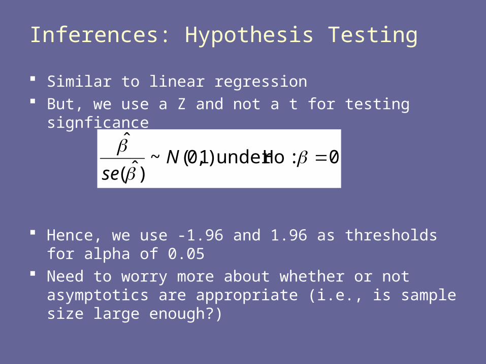
Inferences: Hypothesis Testing
Similar to linear regression But, we use a Z and not a t for testing signficance
Hence, we use -1.96 and 1.96 as thresholds for alpha of 0.05
Need to worry more about whether or not asymptotics are appropriate (i.e., is sample size large enough?)
0 :Hounder )1,0(~)ˆ(
ˆ
Nse

Prostate Example
PSA: p = 0.003 Gleason: p<0.0001
Both PSA and Gleason are strongly associated with capsular penetration
Estimate Std. Error z value Pr(>|z|) (Intercept) -7.639296 1.011128 -7.555 4.18e-14 ***psa 0.026677 0.008929 2.988 0.00281 ** gleason 1.059344 0.158327 6.691 2.22e-11 ***
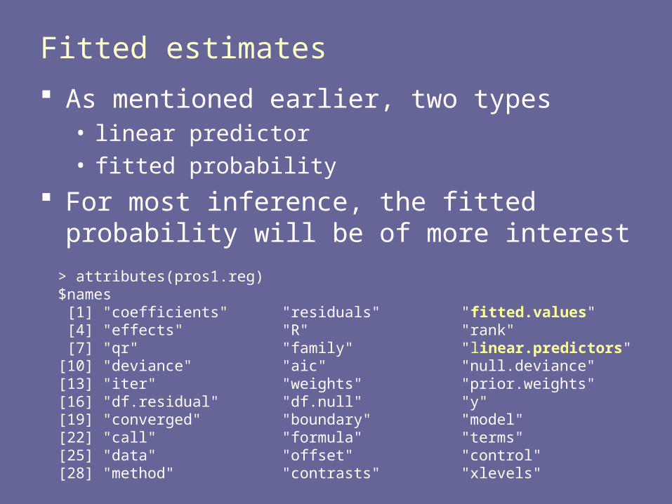
Fitted estimates
As mentioned earlier, two types• linear predictor• fitted probability
For most inference, the fitted probability will be of more interest
> attributes(pros1.reg)$names [1] "coefficients" "residuals" "fitted.values" [4] "effects" "R" "rank" [7] "qr" "family" "linear.predictors"[10] "deviance" "aic" "null.deviance" [13] "iter" "weights" "prior.weights" [16] "df.residual" "df.null" "y" [19] "converged" "boundary" "model" [22] "call" "formula" "terms" [25] "data" "offset" "control" [28] "method" "contrasts" "xlevels"

Fitted values vs. linear predictor
-8 -6 -4 -2 0 2 4 6
0.0
0.2
0.4
0.6
0.8
1.0
pros1.reg$linear.predictor
pro
s1.r
eg
$fit
ted
.va
lue
s
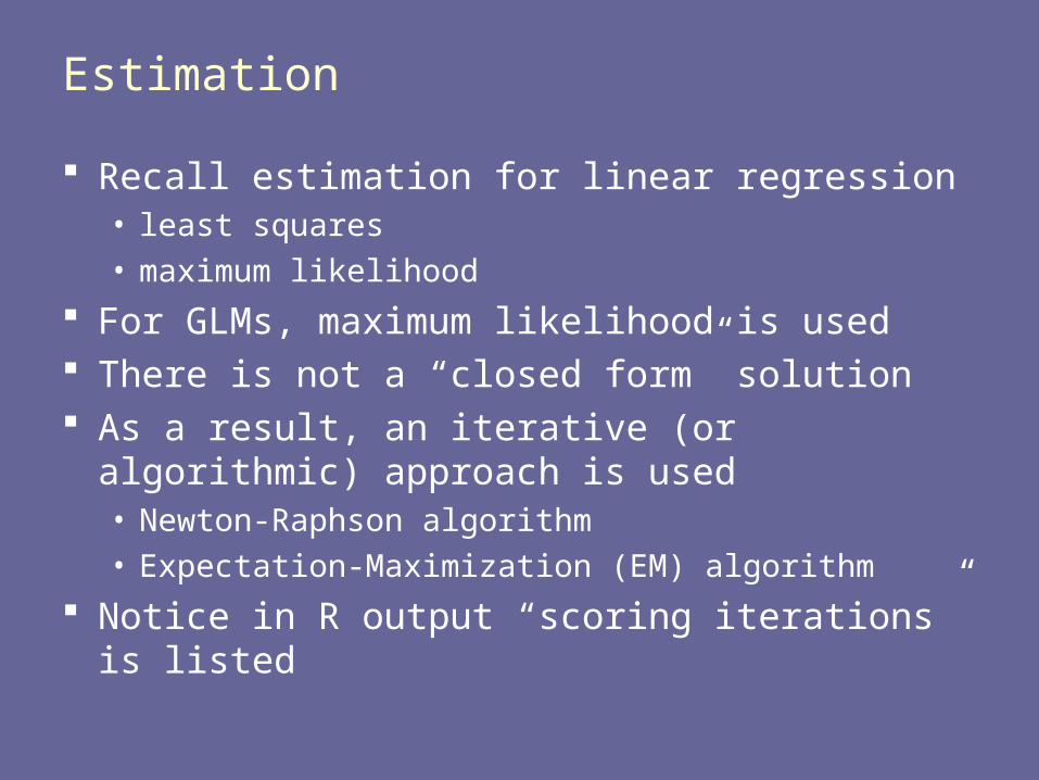
Estimation
Recall estimation for linear regression• least squares• maximum likelihood
For GLMs, maximum likelihood is used There is not a “closed form” solution As a result, an iterative (or algorithmic) approach
is used• Newton-Raphson algorithm• Expectation-Maximization (EM) algorithm
Notice in R output “scoring iterations” is listed
Maximum Likelihood Estimation
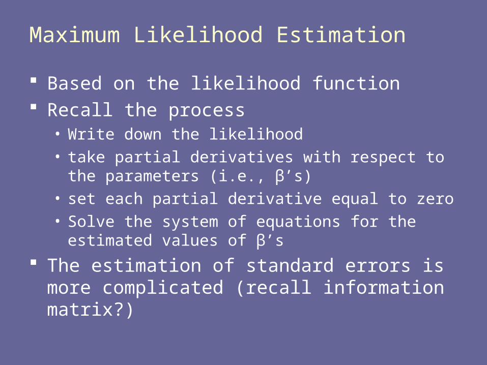
Based on the likelihood function Recall the process
• Write down the likelihood• take partial derivatives with respect to the parameters
(i.e., β’s)• set each partial derivative equal to zero• Solve the system of equations for the estimated
values of β’s
The estimation of standard errors is more complicated (recall information matrix?)

Maximum Likelihood Estimation
With logistic regression (and other generalized linear regression models), you cannot “solve” for the β’s.
You must then use Newton-Raphson (or other) approach to do the solving.
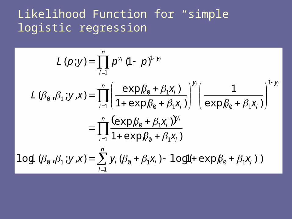
Likelihood Function for “simple” logistic regression
n
iiii
n
i i
yi
n
i
y
i
y
i
i
n
i
yy
xxyxyL
x
x
xx
xxyL
ppypL
i
ii
ii
1101010
1 10
10
1
1
1010
1010
1
1
))exp(1log()(),;,(log
)exp(1
)exp(
)exp(
1
)exp(1
)exp(),;,(
)1();(

Score functions
n
i i
iiii
n
i i
ii
n
iiii
x
xxyx
L
x
xy
L
xxyxyL
1 10
10
1
1 10
10
0
1101010
)exp(1
)exp(log
)exp(1
)exp(log
))exp(1log()(),;,(log
Second derivatives can be obtained to find standard errors and covariances of coefficients.

Data exploration and modeling Scatterplots are not helpful on their own Lowess smooths may be:
0 20 40 60 80 100 120 140
0.0
0.2
0.4
0.6
0.8
1.0
psa
cap
.inv
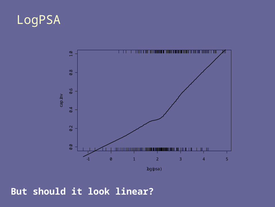
LogPSA
-1 0 1 2 3 4 5
0.0
0.2
0.4
0.6
0.8
1.0
log(psa)
cap
.inv
But should it look linear?

Gleason Score
Smoother? Gleason score is categorical We can estimate the proportion of capsular
penetration for each score
0 2 4 6 8
0.0
0.2
0.4
0.6
0.8
sort(unique(gleason))
gle
aso
n.p

Rcode###########################smoother1 <- lowess(psa, cap.inv)plot(psa, cap.inv, type="n")lines(smoother1, lwd=2)rug(psa[cap.inv==0], side=1)rug(psa[cap.inv==1], side=3)
smoother2 <- lowess(log(psa), cap.inv)plot(log(psa), cap.inv, type="n")lines(smoother2, lwd=2)rug(log(psa[cap.inv==0]), side=1)rug(log(psa[cap.inv==1]), side=3)
###########################gleason.probs <- table(gleason, cap.inv)/as.vector(table(gleason))gleason.p <- gleason.probs[,2]par(mar=c(5,4,1,1))plot(sort(unique(gleason)), gleason.p, pch=16)lines(sort(unique(gleason)), gleason.p, lwd=2)
Modeling, but also model checking
These will be useful to compare “raw data” to fitted model
Smoothers etc can be compared to fitted model If the model fits well, you would expect to see
good agreement Problem?
• only really works for simple logistic regression• cannot generalize to multiple logistic

Revised model
Try logPSA Try categories of Gleason: what makes sense?

pros2.reg <- glm(cap.inv ~ log(psa) + factor(gleason), family=binomial)summary(pros2.reg)
keep <- ifelse(gleason>4,1,0)data.keep <- data.frame(cap.inv, psa, gleason)[keep==1,]
pros3.reg <- glm(cap.inv ~ log(psa) + factor(gleason), data=data.keep, family=binomial)
summary(pros3.reg)
pros4.reg <- glm(cap.inv ~ log(psa) + gleason, data=data.keep, family=binomial)
summary(pros4.reg)
pros5.reg <- glm(cap.inv ~ log(psa) + gleason, family=binomial)summary(pros5.reg)
##########median(log(psa))b <- pros5.reg$coefficientsfit.logpsamed <- b[1] + b[2]*median(log(psa)) + b[3]*c(0:9)phat <- unlogit(fit.logpsamed)lines(0:9, phat, col=2, lwd=3)
b <- pros4.reg$coefficientsfit.logpsamed <- b[1] + b[2]*median(log(psa)) + b[3]*c(0:9)phat <- unlogit(fit.logpsamed)lines(0:9, phat, col=3, lwd=3, lty=2)

Model fit?
0 2 4 6 8
0.0
0.2
0.4
0.6
0.8
sort(unique(gleason))
gle
aso
n.p
Top Related