


Languages
Pages
Legal

Latest laser-wire results
● How does a Laser-Wire work?● Latest ATF results● Focusing optics● Latest PETRA results
University of Oxford: Nicolas Delerue, Brian Foster, David Howell, Myriam Newman, Armin Reichold, Rohan Senanayake, Roman Walczak
Royal Holloway, University of London (RHUL): Grahame Blair, Stewart Boogert, Gary
Boorman, Alessio Bosco, Lawrence Deacon, Pavel Karataev, Michael Price
BESSY: Thorsten Kamps
DESY: Klaus Balewski, Hans-Christoph Lewin, Freddy Poirier, Siegfried Schreiber,
Kay Wittenburg
FNAL: Marc Ross
KEK: Alexander Aryshev, Nobuhiro Terunuma, Junji Urakawa
SLAC: Joe Frisch, Douglas McCormick

● When the photons of a laser interact
with electrons, Compton photons are
produced.
● The number of Compton photons
produced is proportional to the
electrons' density at the position of the
laser.
● By sweeping a laser across an electron
beam one can produce a profile of the
beam and hence measure its size.
● Knowing the size of a beam allow to
measure its emittance.
How does a laser-wire work?
● The resolution of a laser-wire
depends on the size of the laser beam

Laser-wire R&Dfor the ILC
● Many (~70) laser-wires will be used along the ILC to control the
emittance from the source to the Interaction Point.
● Important R&D is needed to demonstrate laser-wire operations in
ILC-like conditions: ultra fast scanning, strong focusing,
high power high rep. rate low M2 laser
● 2 single-pass prototypes in operation:
- One at PETRA (DESY): fast scanning, 2D...
- One at the ATF (KEK): um-resolution
● Other LW applications are investigated by other groups (DR LW,...)

High PowerLASER
2D LW scanner at PETRA
Free space Beam Transport (~ 30m)
Laserrep rate = 20 Hzpulse width 6 ns
Laser spot-size ~ 12 ume- spot size50 – 200 m
Scanning device:Piezo-mirror
max speed 100 Hz
Post IP Imaging Systemaligned for both dimensions
for real time laser size monitoring
Automatic beam findingTranslation stages
2D scanthrough automatic
path selection
Lens f=250mm

0 100 200 300 400 5000,0
0,5
1,0
1,5
2,0
2,5
3,0
Data: A03Soff100TpS_BModel: GaussAmp Equation: y=y0+A*exp(-0.5*((x-xc)/w)^2) Weighting:y No weighting Chi^2/DoF = 0.16595R^2 = 0.73469 y0 0.39407 ±0.0073xc 227.82479 ±0.38993w 62.39258 ±0.51317A 1.9305 ±0.01166
Ca
lori
me
ter
Re
ad
ou
t [V
]
Displacement at IP [um]
Unseeded (100 steps, 100 points per step) 10,000/20Hz = 500sec
0 100 200 300 400 5000,0
0,5
1,0
1,5
2,0
2,5
Data: A23Son100TpSt_BModel: GaussAmp Equation: y=y0+A*exp(-0.5*((x-xc)/w)^2) Weighting:y No weighting Chi^2/DoF = 0.06425R^2 = 0.81966 y0 0.43568 ±0.0036xc 281.70086 ±0.25261w 46.59614 ±0.29214A 1.61997 ±0.008
Displacement at IP [um]
Cal
orim
eter
Rea
dout
[V]
Seeded (100 steps, 100 points per step) 10,000/20Hz = 500sec
Sigma ~ 46umSigma ~ 62um
Scan give a better resolution when the laser is seeded.
Alessio Bosco & Michael Price

0 100 200 300 400 500
0,2
0,4
0,6
0,8
1,0
1,2
1,4
1,6
1,8
2,0
2,2
Data: A21Son1TpStep_BModel: GaussAmp Equation: y=y0+A*exp(-0.5*((x-xc)/w)^2) Weighting:y No weighting Chi^2/DoF = 0.06544R^2 = 0.81187 y0 0.43749 ±0.03785xc 278.99107 ±2.70148w 49.22143 ±3.21538A 1.54167 ±0.07906
Ca
lori
me
ter
Re
ad
ou
t [V
]
Displacement at IP [um]
Seeded (100 steps, 1 point per step) 100/20Hz = 5 sec
0 100 200 300 400 5000,0
0,5
1,0
1,5
2,0
2,5
Data: A22Son10TpSte_BModel: GaussAmp Equation: y=y0+A*exp(-0.5*((x-xc)/w)^2) Weighting:y No weighting Chi^2/DoF = 0.06594R^2 = 0.81565 y0 0.42243 ±0.01192xc 284.69625 ±0.83171w 48.65234 ±0.97817A 1.59288 ±0.02501
Ca
lori
me
ter
Re
ad
ou
t [V
]
Displacement at IP [um]
Seeded (100 steps, 10 points per step) 1,000/20Hz = 50sec
Sigma ~ 49um
Sigma ~ 49um
0 100 200 300 400 5000,0
0,5
1,0
1,5
2,0
2,5
Data: A23Son100TpSt_BModel: GaussAmp Equation: y=y0+A*exp(-0.5*((x-xc)/w)^2) Weighting:y No weighting Chi^2/DoF = 0.06425R^2 = 0.81966 y0 0.43568 ±0.0036xc 281.70086 ±0.25261w 46.59614 ±0.29214A 1.61997 ±0.008
Displacement at IP [um]
Ca
lori
me
ter
Re
ad
ou
t [V
]
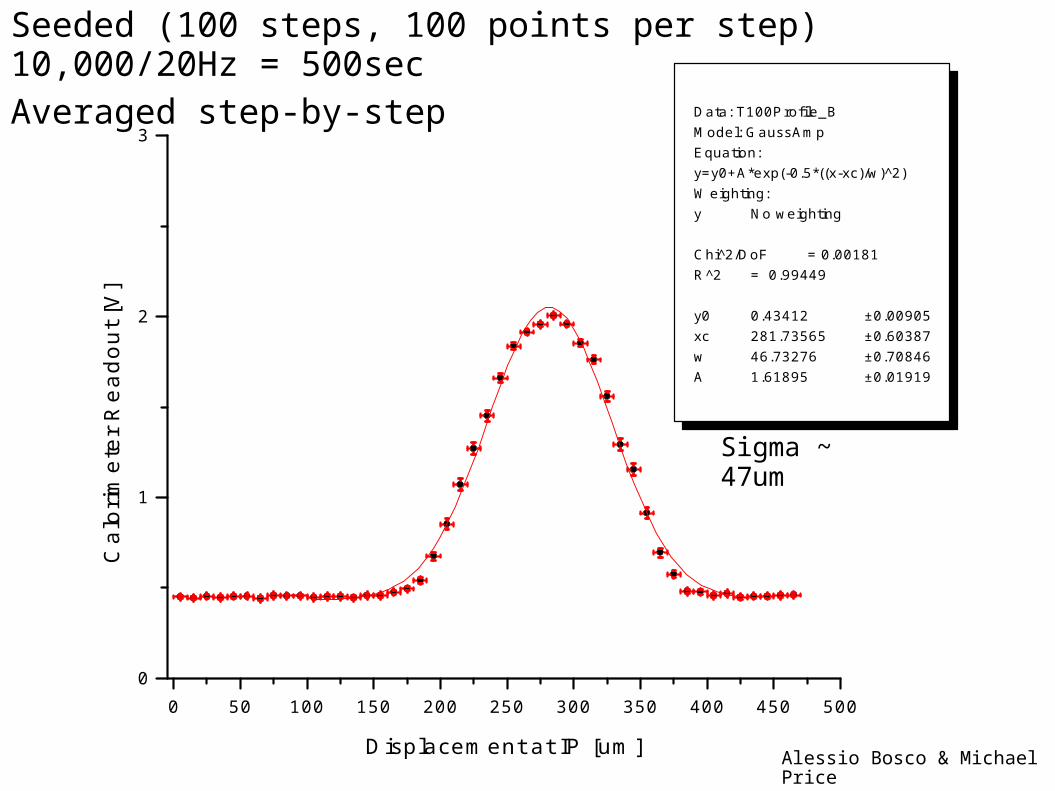
Seeded (100 steps, 100 points per step) 10,000/20Hz = 500sec
Sigma ~ 47um
Fast scans give a resolution comparable to scans with more data points
0 50 100 150 200 250 300 350 400 450 5000
1
2
3Data: T100Profile_BModel: GaussAmp Equation: y=y0+A*exp(-0.5*((x-xc)/w)^2) Weighting:y No weighting Chi^2/DoF = 0.00181R^2 = 0.99449 y0 0.43412 ±0.00905xc 281.73565 ±0.60387w 46.73276 ±0.70846A 1.61895 ±0.01919
Ca
lori
me
ter
Re
ad
ou
t [V
]
Displacement at IP [um]
Seeded (100 steps, 100 points per step) 10,000/20Hz = 500secAveraged step-by-step
Sigma ~ 47um
Alessio Bosco & Michael Price

ATF Extraction line laser-wire
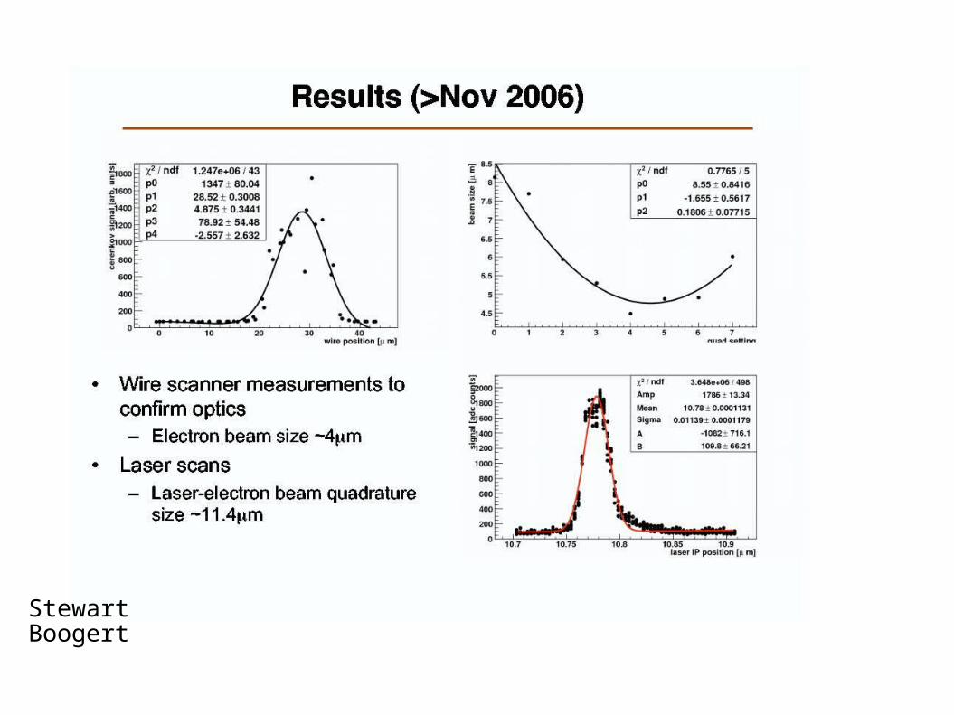
● Goal: demonstrate um-scale resolution in a single pass system
● System successfully installed and tested last year with a commercial lens
● Strong focusing lens will be installed this year
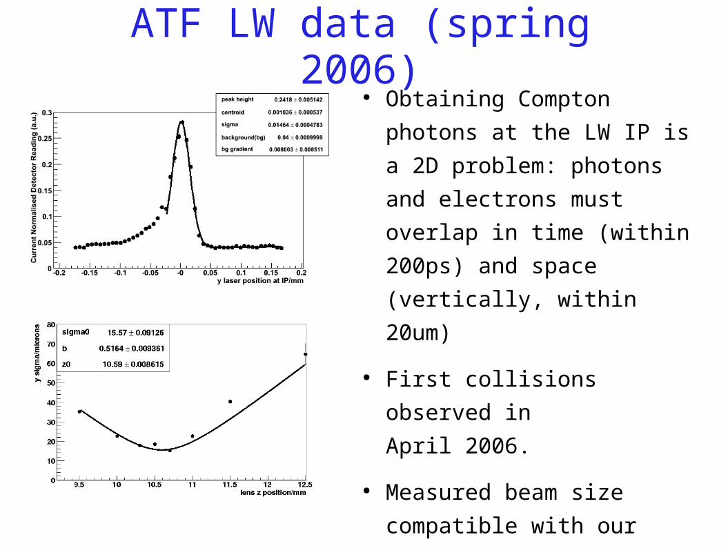
ATF LW data (spring 2006)● Obtaining Compton photons at the
LW IP is a 2D problem: photons
and electrons must overlap in time
(within 200ps) and space
(vertically, within 20um)
● First collisions observed in
April 2006.
● Measured beam size compatible
with our expectations.
● Scan asymmetry due to lens
aberrations
● Laser M2 ~ 2.9
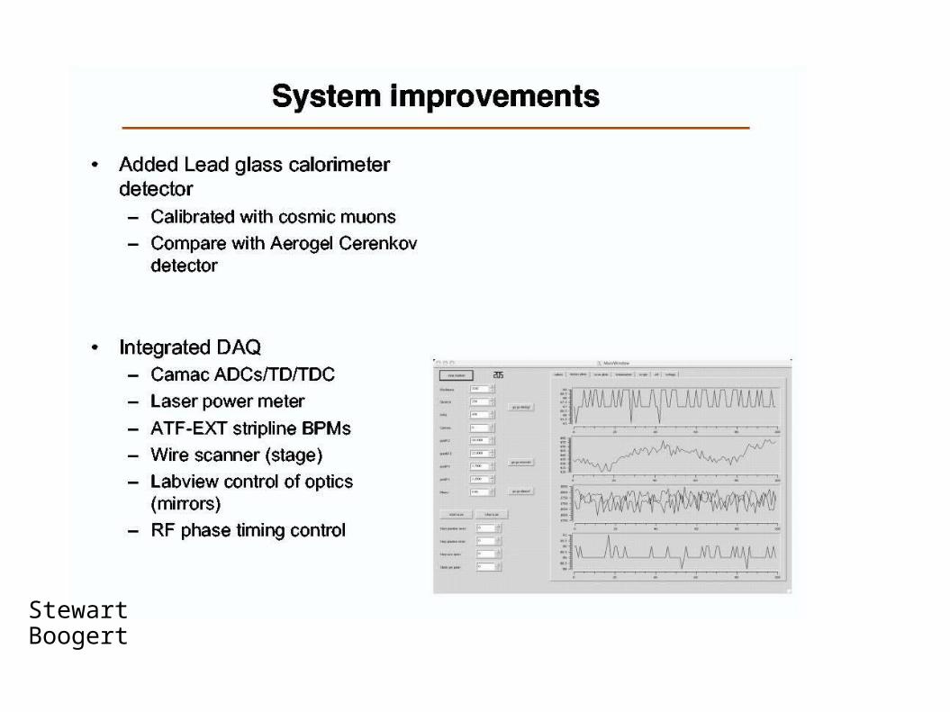
Stewart Boogert
Stewart Boogert

Lawrence Deacon
Cerenkov detector
Photon detector comparison
LW Scans 13th December 2006
Calorimeter

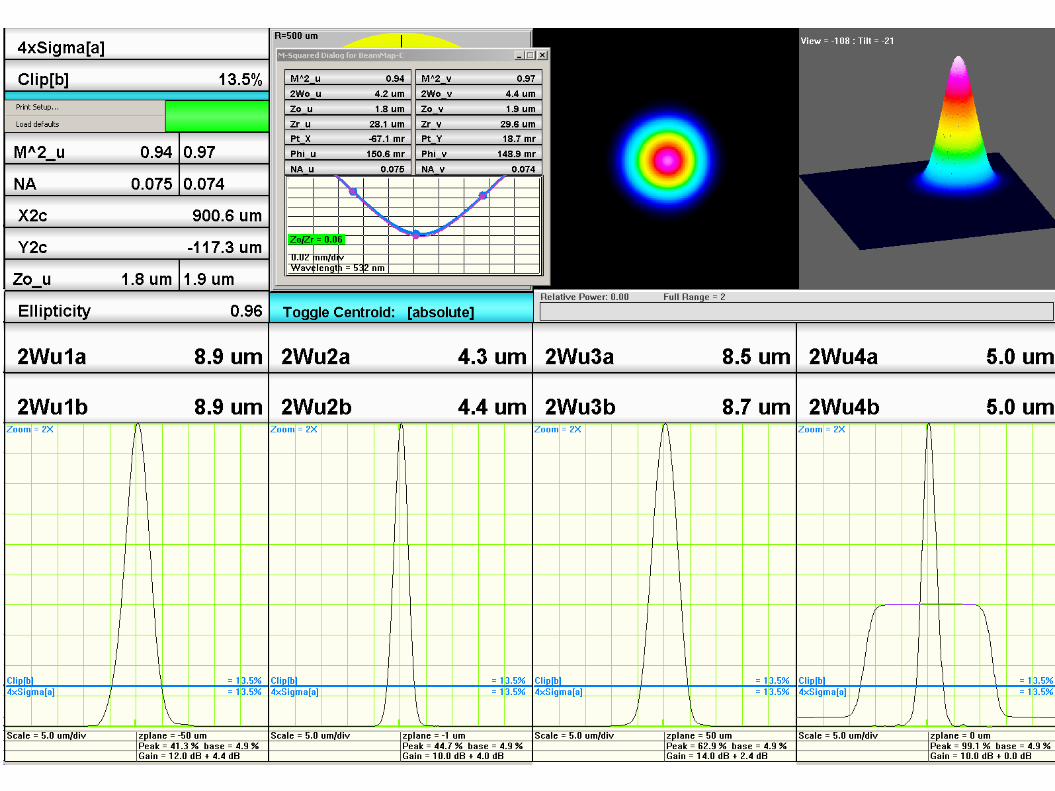
f/2 lens design@532nm● Focal length: 56mm
● One aspheric
element, one flat
● Back focal length:
24mm
● Aperture f/2
● All elements in fused
silica
● No primary ghosts,
one secondary ghost
● Expected spot radius
~2 micrometres
A low f# lens is needed to reach um-scale resolution.

Lens profiling● A precise measurement of the characteristic of the lens as
produced is necessary.
● A commercial lens with known properties has been used as benchmark of the test setup.
● Profile measurements with a knife-edge scanner confirm the expected performances.
laser
Wave plate
Telescope
1% beam splitter
mirror
lens
window
Beam profiler
mirror
mirror
mirror
10% beam splitterLaser M2 ~1.1, Parallel beam, 8.5mm diameter Myriam Newman
Laser development
● Need a high power high repetition rate laser● Mode quality is very important to achieve good
resolution● => Fibre laser technology with chirped pulse
amplification (CPA) best suited for our needs.● Currently discussing possible systems with
several companies

Outlook● Two laser-wire prototypes are now operational
for ILC related R&D ● 2D scans will soon be attempted with the PETRA
system● Strong focusing lens (f/2) performances are being
measured ● ATF LW mechanical hardware is being upgraded
for the installation of the strong focusing lens● Laser technology & design have been chosen
Top Related