


Languages
Pages
Legal

V1.8 11/20/00 Accepted for Publication, Journal of Geophysical Research.
1
Landslide Tsunami
Steven N. Ward
Institute of Geophysics and Planetary Physics
University of California at Santa Cruz
Santa Cruz, CA 95064 USA
Abstract
In the creation of “surprise tsunami”, submarine landslides head the suspect list. Moreover,
improving technologies for seafloor mapping continue to sway perceptions on the number and
size of surprises that may lay in wait offshore. At best, an entirely new distribution and mag-
nitude of tsunami hazards has yet to be fully appreciated. At worst, landslides may pose seri-
ous tsunami hazard to coastlines worldwide, including those regarded as immune. To raise the
proper degree of awareness, without needless alarm, the potential and frequency of landslide
tsunami have to be assessed quantitatively. This assessment requires gaining a solid under-
standing of tsunami generation by landslides, and undertaking a census of the locations and
extent of historical and potential submarine slides. This paper begins the process by offering
models of landslide tsunami production, propagation and shoaling; and by exercising the the-
ory on several real and hypothetical landslides offshore Hawaii, Norway and the United States
eastern seaboard. I finish by broaching a line of attack for the hazard assessment by building
on previous work that computed probabilistic tsunami hazard from asteroid impacts.
1. Introduction
Earthquakes generate most tsunami. Rightly so,
tsunami research has concentrated on the hazards
posed by seismic sources. The past decade how-
ever, has witnessed mounting evidence of tsu-
nami parented by submarine landslides. In fact,
submarine landslides have become prime sus-
pects in the creation of “surprise tsunami” from
small or distant earthquakes. As exemplified by
the wave that devastated New Guinea's north
coast in 1998 (Tappin, et. al., 1999; Geist, 2000),
surprise tsunami can initiate far outside of the
epicentral area of an associated earthquake, or be
far larger than expected given the earthquake
size. In contemplating the great number and im-
mense extent of seabed failures known to have
frequented recent geological history, the biggest
surprise just may arrive without any precursory
seismic warning at all -- a tsunami sprung from a
spontaneous submarine landslide.
The geography of earthquakes only casually
resembles the geography of submarine landslides.
Tsunami excitation mechanisms between earth-
quakes and landslides differ substantially too.
Accordingly, an entirely new distribution and
magnitude of tsunami hazards has yet to be fully
Ward: Landslide Tsunami 2
appreciated. Landslides may pose perceptible
tsunami hazards to areas regarded as immune –
the Gulf of Mexico, the North Sea, or the eastern
seaboard of the United States. Many of these ar-
eas, unaccustomed to earthquakes and earthquake
tsunami, lie on flat and passive continental mar-
gins. A 5-meter sea wave striking there would
over-run far more territory than a similar wave
hitting a rugged shore, such as California's north
coast.
To raise a proper degree of awareness, without
needless alarm, the potential and frequency of
landslide tsunami must be assessed quantitatively.
To make this assessment, geophysicists must first
garner an understanding of tsunami generation by
landslides equal to what they know about tsunami
generation by earthquakes. Second, geologists
and oceanographers must undertake a census of
the locations and sizes of historical and potential
submarine landslides, and estimate their occur-
rence rates. Setting the stage for a quantitative
hazard analysis, this paper begins to tackle step
#1 above by offering elementary models of land-
slide tsunami production, propagation and shoal-
ing; and by exercising the theory on several real
and hypothetical cases.
2. Tsunami characteristics under lineartheory.
The tsunami computed in this article derive
from classical theory. Classical tsunami theory
envisions a rigid seafloor overlain by an incom-
pressible, homogeneous, and non-viscous ocean
subjected to a constant gravitational field. Fur-
thermore, I confine attention to linear theory.
Linear theory presumes that the ratio of wave
amplitude to wavelength is much less than one,
but it does not otherwise restrict tsunami wave-
length. In particular, I do not make a long
wave/shallow water assumption.
Linear wave theory may not hold in every
situation, but in the application here, the assump-
tion of linearity presents far more advantages than
draw-backs. Foremost among the advantages is
superposition. Superposition means that complex
tsunami waveforms can be spectrally decom-
posed, independently propagated, and then recon-
structed. Superposition also means that complex
landslide sources can be synthesized from simple
ones. For all but monster landslides, linear theory
breaks down only during the final stage of tsu-
nami shoaling and inundation when the wave
height exceeds the water depth (Synolakis, 1987).
Taking waves the last mile to the beach does re-
quire full hydrodynamic calculation; however, if
one is willing to stand off a bit in water no shal-
lower than the height of the incoming waves, then
linear theory should work fine. If nothing else,
linear theory fixes a reference to compare predic-
tions from various non-linear approaches.
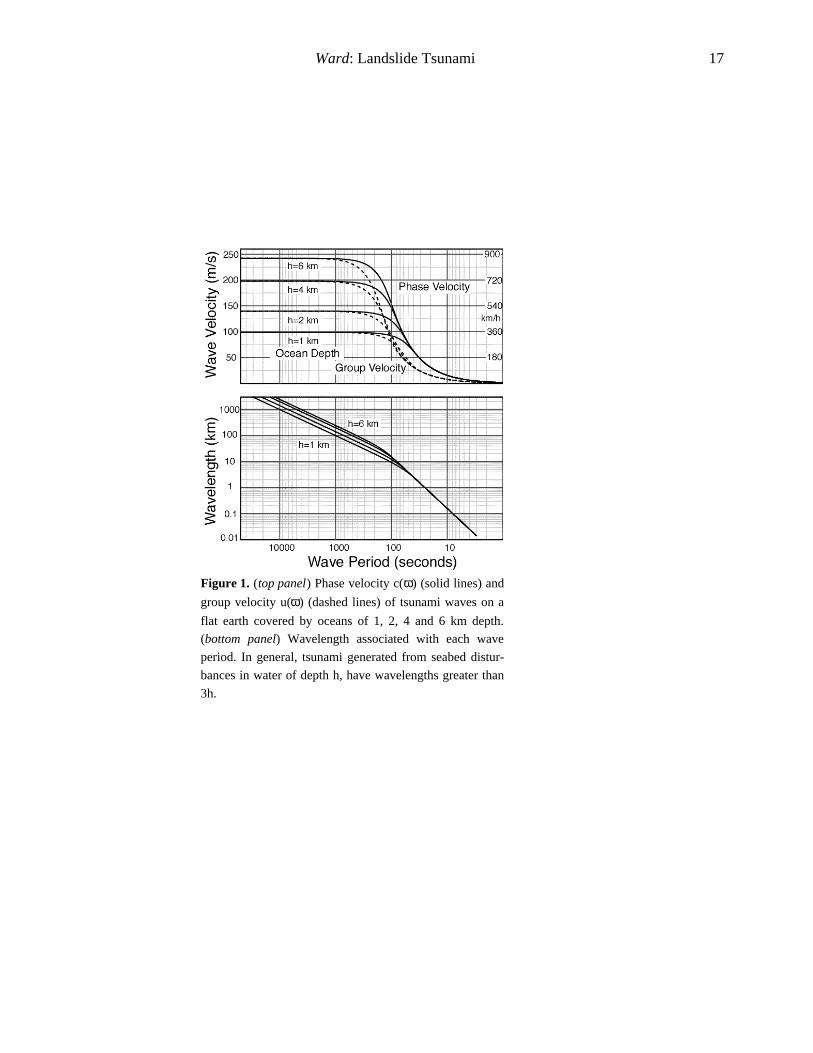
In classical theory, the phase c(ω), and group
u(ω) velocity of surface gravity waves on a flat
ocean of uniform depth h are
c( ) =gh tanh[k( )h]
k( )h (1)
and
u( ) = c( )1
2+
k( )h
sinh[2k( )h]
(2)
Here, g is the acceleration of gravity (9.8 m/s2)
and k(ω) is the wavenumber associated with a sea
Ward: Landslide Tsunami 3
wave of frequency ω. Wavenumber connects to
wavelength λ(ω) as λ(ω)=2π/k(ω). Wavenumber
also satisfies the dispersion relation
2 = gk( )tanh[k( )h] (3)
For surface gravity waves spanning 1 to 50,000 s
period, Figure 1 plots c(ω), u(ω), and λ(ω). These
quantities vary widely, both as a function of
ocean depth and wave period.
3. Excitation of Tsunami by Sea Floor up-lift
Suppose that the seafloor at points r0 uplift in-
stantaneously at time τ(r0) by amount u zbot (r0).
Under classical tsunami theory in a uniform
ocean of depth h, this bottom disturbance stimu-
lates surface tsunami waveforms (vertical com-
ponent) at observation point r=x ˆ x +y ˆ y and time t
of (Ward, 2000)
u zsurf(r,t) = Re dk
ei[ k• r− ( k ) t ]
4 2 cosh(kh)F(k)
k∫
with
F(k) = dr0 u zbot (r0 , (r0 ))e
r0
∫−i[ k• r0 − (k) ( r0 )]
(4a,b)
In (4), k=|k|, ω2(k) = gktanh(kh), dk=dkxdky,
dr0=dx0dy0, and the integrals cover all wavenum-
ber space and locations r0 where the seafloor
disturbance u zbot (r0)≠0.
Equation (4a) has three identifiable pieces:
a) The F(k) term is the wavenumber spectrum
of the seafloor uplift. This number relates to the
amplitude, spatial, and temporal distribution of
the uplift. Tsunami trains (4a) are dominated by
wavenumbers in the span where F(k) is greatest.
The peak of F(k) corresponds to the characteristic
dimension of the uplift. Usually, large-
dimensioned landslides produce longer wave-
length, hence lower frequency tsunami than
small-dimensioned sources.
b) The 1/cosh(kh) term low-pass filters the
source spectrum F(k). (1/cosh(kh)→1 when
kh→0, and 1/cosh(kh)→0 when kh→∞, so the
filter favors long waves.) Because of the low-pass
filter effect of the ocean layer, only wavelengths
of the uplift source that exceed three times the
ocean depth (i.e. kh=2πh/λ<≈2) contribute much
to a tsunami.
c) The exponential term in (4a) contains all of
the propagation information including travel time,
geometrical spreading, and frequency dispersion.
By rearranging equations (4a,b) as a Fourier-
Bessel pair, vertical tsunami motions at r can also
be written as
uzsurf (r, t )= Re
k dk e−iω ( k ) t
2π cosh(kh)Jn (kr)
n=−∞
∞
∑ einθ Fn (k)0
∞
∫with (5)
Fn (k) = dr0 uzbot(r0) Jn (kr0 )
r 0
∫ e i(ω(k)τ(r0 )−nθ0 )
Here, θ and θ0 mark azimuth of the points r and
r0 from the ˆ x axis, and the Jn(x) are cylindrical
Bessel functions. Although (4) and (5) return
identical wavefields, for certain simply distrib-
uted uplift sources (e.g. point dislocation models
of earthquakes), (5) might be easier to evaluate
Ward: Landslide Tsunami 4
than (4). For instance, for radially symmetric up-
lifts with τ(r0)=0, all of the terms in the sum save
F0(k) vanish, and (5) becomes
u zsurf(r,t) =
k dk cos[ (k)t]
2 cosh(kh)J0 (kr)F0 (k)
0
∞
∫
Fundamental formulas (4) and (5) presume in-
stantaneous seafloor uplift at each point. This
does not mean that landslides modeled by these
formulas happen all at once. The function τ(r0)
that maps the spatial evolution of the slide is un-
restricted. Actually, the distinction between in-
stantaneous uplift and uplift over several, or sev-
eral tens of seconds is not a big issue. Dominant
tsunami waves produced from landslides even in
fairly shallow water have periods exceeding 100
seconds. Uplifts taking several seconds to de-
velop still look “instantaneous”. If the distinction
ever does become significant, superposition per-
mits convolution of solutions (4) with "box car"
functions to spread the uplift at a point over a fi-
nite rise time TR as
uzsurf (r, t )= TR
-1 dˆ t t - TR
t
∫ Re dkei [k •r−ω ( k )̂ t ]
4π2 cosh(kh)F(k) (6)
k∫
4. Tsunami excitation from a simple slide.
A good way to get a feeling for the factors
governing landslide tsunami production is to con-
sider a simple slide confined to a rectangle of
length L and width W. To mimic the progression
of a landslide disturbance, let a constant uplift u0
(the slide thickness) start along one width of the
rectangle and run down its length (the ˆ x direc-
tion, say) at velocity vr, i.e. τ(r0)=x0/vr . Placing
this u zbot
(r0) and τ(r0) into (4b) gives
F(k) = u0 dy0e− iky y0
-W/2
W/2
∫ dx0 e− i[k x − (k)/vr ]x0
0
L(t)
∫ (7)
with kx = k • ˆ x and ky = k • ˆ y . The tsunami
waves from a simple slide at observation point rand time t are
uzsurf (r, t )=
u0L(t)W
4π2
× Re dke i (k •r−ω ( k ) t )e− iX( k )
cosh(kh)
sinX(k)
X(k)
sinY(k)
Y(k)k∫ (8)
where
X(k) =kL(t)
2ˆ k • ˆ x −c(k)/v r( ) ; Y(k) =
kW
2ˆ k • ˆ y ( )
and L(t)=min[L,vrt] for t≥0 and L(t)=0 for t<0.
Recognize the leading multiplier in (8) u0L(t)W,
as the volume of the uplift. Clearly, landslide
volume carries first order importance in tsunami
production. The X(k) and Y(k) terms, because
they depend on the relative positions of the ob-
servation point and the landslide source, instill
radiation patterns to the tsunami. Elements in the
radiation patterns include the length and width of
the slide, the slide velocity, the tsunami speed,
and the orientation of the slide relative to the
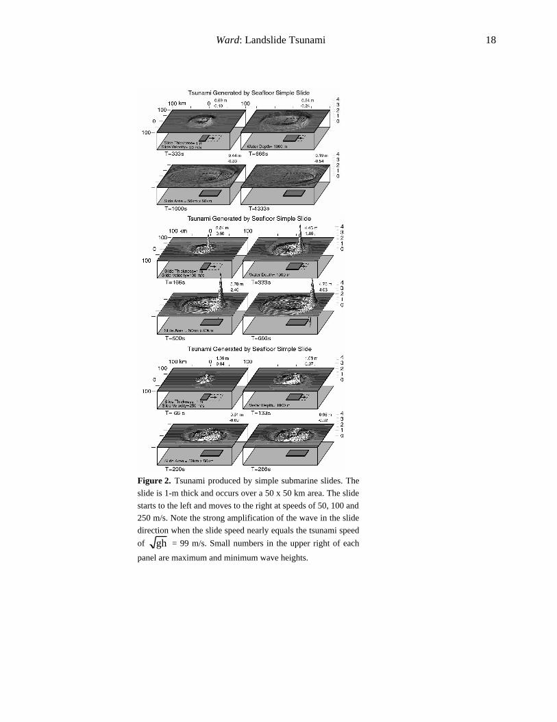
sample point. Figure 2 pictures tsunami computed
from (8) when a 50 x 50 km seafloor patch pro-
gressively uplifts by 1 m. The uplift starts along
the left edge of the slide patch and moves to the
right. The panels in Figure 2 snapshot the situa-
tion at t= 1/3, 2/3, 3/3 and 4/3 multiples of the
slide duration L/vr. Calculations like these reveal
that, depending on the aspect ratio of the land-
slide and the ratio of slide velocity to the tsunami
phase velocity, significant beaming and amplifi-
cation are possible. In particular, as the slide ve-
Ward: Landslide Tsunami 5
locity vr approaches the tsunami speed c(k)≈ gh ,
then X(k) is nearly zero for waves travelling in
the slide direction. For observation points in this
direction, the waves from different parts of the
source arrive “in phase” and constructively build.
Figure 2 highlights these beaming and amplifica-
tion effects. Witness the large tsunami pulse that
can be sent off in the direction of the slide. The
tsunami peak in the middle panel stands nearly
six times the thickness of the slide. Such extreme
amplifications however, localize to a narrow
swath in the forward direction.
Maximum Amplitude.
Figure 3 summarizes many experiments like
Figure 2 in graphs of peak tsunami height at the
toe of a simple slide (dots at top of figure) versus
slide velocity, slide dimension and water depth.
As in any wave excitation problem, the most effi-
cient generators operate at frequencies and
wavelengths that correspond to the waves in
question. Figure 1 shows that in 1000 m of water,
tsunami waves of length L=50 km for instance,
prefer to be excited at 500 second period. For
very slow slides L/vr>>L/ gh , tsunami produc-
tion tends toward zero. For very fast slides
L/vr<<L/ gh , tsunami height tends toward the
slide thickness. Slides that move at velocities
close to the tsunami speed amplify the sea waves
because the wavelength and period of excitation
are synchronized to the preferred values. Even for
slow-moving events, the steepness of the re-
sponse curves on either side of their peak be-
speaks the importance of slide velocity in tsunami
prediction. For example, Figure 3 forecasts that a
slide moving at 0.2 gh produces waves twice as
large as a slide moving 0.1 gh . Figure 3 also
documents the tendency for larger slide volumes
to generate higher waves (as expected from equa-
tion (8)) and the tendency of deeper oceans to sti-
fle wave amplitude by means of the 1/cosh(kh)
low pass filter.
5. Complex slides
Tsunami from the simple slides in Figures 2
and 3 crystallize the roles of slide volume, dimen-
sion, velocity and water depth on tsunami pro-
duction. Simple slides however, may not be suit-
able for many applications. Most notably, the
simple slide entails a net volume change at the
sea floor. Except when part of the slide material
originates above sea level, deposition (uplift)
should equal excavation (subsidence). Fortu-
nately, because of linearity, simple slides can be
combined into complex ones. The first panel in
Figure 4 pictures the simple slide. A block de-
tachment (panel 2) forms from the combination of
a simple slide and a trailing “negative” simple
slide of equal thickness and velocity. Run-out
slides (panels 3 and 4) resemble detachments,
however the block disintegrates as it slides. I find
run-out slides to be more flexible than block de-
tachments in modeling realistic situations because
the area, shape and thickness of the excavation
can differ from the area, shape and thickness of
the region covered. In Run-out Slide Type 1, a
thick block disintegrates at its front and runs out
in a thinner layer. Run-out Slide Type 1 too,
forms from a pair of simple slides – a leading
positive one trailed by a negative thicker one. In
run-out models where the front and back slides
have different thickness, the two slides must ad-
vance at different speeds to conserve volume
rates of excavation and deposition. Run-out Slide
Ward: Landslide Tsunami 6
Type 2 (panel 4, Figure 4) also begins as a de-
tachment, but the block disintegrates in such a
way as to leave a trail of debris. The disintegra-
tion mechanism resembles a pushed deck of cards
that drops in turn, each bottom one. The fifth and
sixth panels of Figure 4 portray “sand pile” slides.
These exemplify a different class of failure in that
the instability nucleates at the toe and works its
way up slope. Channel deposits often "flush out"
in sand pile fashion. Unlike avalanche-like slides,
the up-slope propagation in sand pile failures can
beam tsunami toward shore.
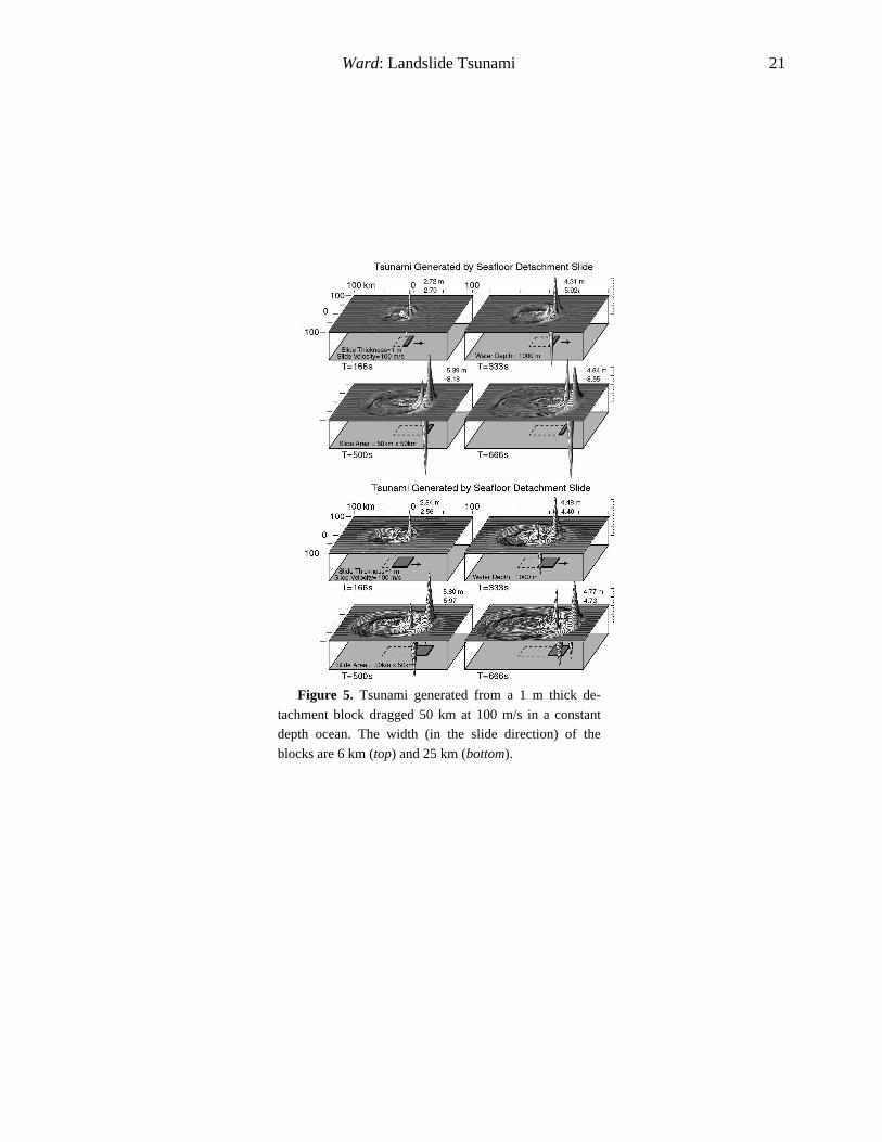
Figure 5 shows tsunami stirred from detach-
ment blocks 50 km wide, slid over 50 km of sea-
floor at a velocity of 100 m/s in a constant depth
ocean. The times pictured are at 1/3, 2/3, 3/3 and
4/3 multiples of the 500 s slide duration. In the
top and bottom panels, the block has length (par-
allel to the slide direction) of 6 and 25 km re-
spectively. Block detachments, being the sum of
positive and negative simple slides, spawn double
pulsed tsunami – a positive wave in front fol-
lowed by a negative wave of equal size. Early on,
long or thin block detachments look to be equally
efficient tsunami generators as the simple slide
(middle Figure 2), provided that they cover the
same distance at the same speed, and the length
of the block is larger than the ocean depth. When
double-pulsed waves propagate to distance how-
ever, the fastest components of the trailing nega-
tive pulse over take the slower components of the
positive pulse. Tsunami from block detachments
attenuate faster than waves from a simple slide.
6. Green’s function approach
Tsunami computed from the simple slide and
its variants are illuminating, but inflexible be-
cause they are restricted to rectangles of uniform
uplift and slide velocity in an ocean of fixed
depth. An obvious work-around uses a pseudo
Green’s function method that computes tsunami
from sums of many small simple slides of differ-
ent thickness, length, width, slide velocity, ori-
entation and initiation time, placed under seas of
changing depth. A generalization of (8) casts tsu-
nami Green's functions at r and time t from an
elemental simple slide at r0 and initiation time t0
as
Gzsurf(r,r0 , t , t0 ) = u0L0 (t − t0 )W0
4π2
× Rekdke−iω 0 (k)(t − t 0 )
cosh[kh(r0 )]0
∞
∫
× dφ0
2π
∫ eik r-r0 cos( θ−φ )
e− iX(k, φ ) sinX(k,φ)
X(k,φ)
sinY(k,φ)
Y(k,φ)
(9)
In (9), θ is the azimuth between the vector r-r0
and the slide direction,
X(k,φ) = ω0( k ) L0 (t − t0 )
2v r
vr cosφc0(k)
− 1
;
Y(k,φ) =kW0
2sin φ
(10)
and L0(t-t0)=min[L0,vr(t-t0)] for (t-t0)≥0 and L0(t-
t0)=0 for (t-t0)<0. Dimensions L0 and W0 of the
elemental sources are selected as small as needed
to reproduce adequately structural variations over
dimensions L and W of the whole slide. Antici-
pating that ocean depth atop the slide will be one
such variation, I make specific in (9) that
ω0(k)=ω(k,h(r0)) and c0(k)=c(k,h(r0)) =ω0(k)/k are
the frequency and phase velocity associated with
Ward: Landslide Tsunami 7
fixed wavenumber k in water depth h(r0), and that
h(r0) appears in the 1/cosh[kh] filter. These ex-
tensions between (8) and (9) account for the ef-
fects of the slope over which the slide moves.
A Green's function approach evaluates (9) for
several dozen elemental slides at each observa-
tion point r and time t. Because (9) includes a
double integration, repeated evaluation of it
makes for heavy computing. However, if the dis-
tance to most of the observation sites dwarfs the
size of the elemental slides (several km square
usually), then the calculation can be sped by pre-
suming that only waves directed toward the ob-
server (along a ray path) at azimuth θ contribute
significantly. That is, in the bracketed radiation
pattern term in (9), integration variable φ can be
replaced by ray azimuth θ as
Gzsurf(r,r0 , t , t0 ) ≈ u0L0(t − t0)W0
4π2
× Rekdk e−i[ω 0 ( k ) ( t−t 0 )+X(k, θ)]
cosh[kh(r0)]0
∞
∫
×sinX(k,θ)
X(k,θ)
sinY(k,θ)
Y(k,θ)dφ
0
2π
∫ eik r-r0 cos( θ−φ )
(10)
Note that there may be more than one ray that ties
the source and receiver. The identity
2πJ 0(k r - r0 ) = dφ0
2π
∫ eik r-r0 cos(θ − φ)
collapses the double integration to a single inte-
gration
Gzsurf(r,r0 , t , t0 ) ≈ u0L0(t − t0)W0
2π
×kdk J 0(k r - r0 )cos[ω0(k)(t − t0) +X(k,θ)]
cosh[(kh(r0 )]0
∞
∫
×sinX(k,θ)
X(k,θ)
sinY(k,θ)
Y(k,θ)(11)
Tsunami u zsurf(r,t) from landslides of any shape,
any velocity, and any thickness are constructed
by integrating the Green's functions over the area
of the slide
u zsurf(r,t) = dr0u0
bot(r0 )Gzsurf(r,r0 , t , t0 (r0 ))
r0
∫ (12)
Computing (12) for all r, t and ro needs hun-
dreds of Gzsurf (r,r0, t , t0(r0)), so it is worthwhile to
optimize integration (11) that consumes most of
the effort. First, recognize the senselessness of
carrying the wavenumber integration past
kmax=2π/h(r0) because the 1/cosh[kh(r0)] low pass
filter eliminates shorter wavelengths. Second, for
each elemental slide, an efficient strategy em-
ploys the same set of k values in integration (11)
for all observer locations r. This way, many terms
like ω0(k) and kdk/cosh(kh(r0)) can be computed
once, grouped, and retained. Third, take care in
the selection of step size dk. Too large a step ali-
ases the signal. Too small a step wastes resources.
7. Tsunami Propagation
In uniform depth oceans, tsunami propagate
out from landslides in circular rings with ray
paths that look like spokes on a wheel. In real
oceans, tsunami speeds vary place to place (even
at a fixed frequency). Tsunami ray paths refract
and bend. Consequently, in real oceans, both tsu-
Ward: Landslide Tsunami 8
nami travel time and amplitude have to be ad-
justed relative to their values in uniform depth
ones. To do this, it is best to transform the various
integrals over wavenumber to integrals over fre-
quency because wave frequency, not wavenum-
ber, is conserved throughout. Using the relations
u(ω)=dω/dk and c(ω)=ω/k(ω), Tsunami Green's
functions (11) in variable depth oceans are to a
good approximation
Gzsurf(r,r0 , t , t0 ) ≈ u0L0(t − t0)W0
2π
×k0(ω)dω J0(ωT(ω,r,r0 ))cos[ω(t − t0 ) +X(ω,θ)]
u0(ω)cosh[(k0 (ω)h(r0 )]0
∞
∫
×sinX(ω ,θ)
X(ω,θ)
sinY(ω ,θ)
Y(ω,θ)G(r,r0)SL(ω,r ,r0)
(13)
where
X(ω,θ) = ωL0(t − t0)
2vr
v r cosθc0(ω)
−1
;
Y(ω,θ) = ωW0
2c0(ω)sinθ
Again, with subscript 0, I make specific that
k0(ω)=k(ω,h(r0)), c0(ω)=c0(ω,h(r0))=ω/k0(ω), and
u0(ω)=u0(ω,h(r0)) are the wavenumber, phase and
group velocity associated with frequency ω in
water of depth h(r0).
In passing from (11) to (13), the travel time
of waves of frequency ω has changed from |r-
r0|/c(ω) to
T(ω,r ,r0) = d p / c (ray path∫ ω, h (p)) (14)
where the integration path traces the tsunami ray
from the source to the observation point. To side-
step tracing rays and evaluating integral (14) at
every frequency in (13), a short cut --
1) Evaluates T(ω = 0,r,r0) = dp/ gh(p)r a y p a t h
∫2) Finds an equivalent ocean depth h (r,r0 ) along
the ray path of length P(r,r0),
h (r,r0 ) = P 2(r,r0 )/gT2 (0,r,r0 )
3) Determines the wavenumber k(ω,h (r,r0 )) as-
sociated with the equivalent ocean depth by
solvingω2 = gk(ω, h (r,r0 ))tanh[k(ω, h (r,r0 ))h (r,r0 )]
and 4) Approximates the path and frequency de-
pendent travel time by
T(ω,r ,r0) = P(r,r0 )k(ω, h (r,r0 ))/ ω
Equation (13) also incorporates new geometri-
cal spreading G(r,r0), and shoaling factors
SL(ω,r,r0). In a flat, uniform ocean, the function
J0(k|r-r0|) imparts a 1/ r amplitude loss to tsu-
nami due to geometrical spreading. The new
factor
G(r,r0) =P(r,r0 )L(rξ )
P(rξ ,r0)L(r) (15)
adjusts the 1/ r attenuation to account for topog-
raphic refraction that makes wave amplitudes lo-
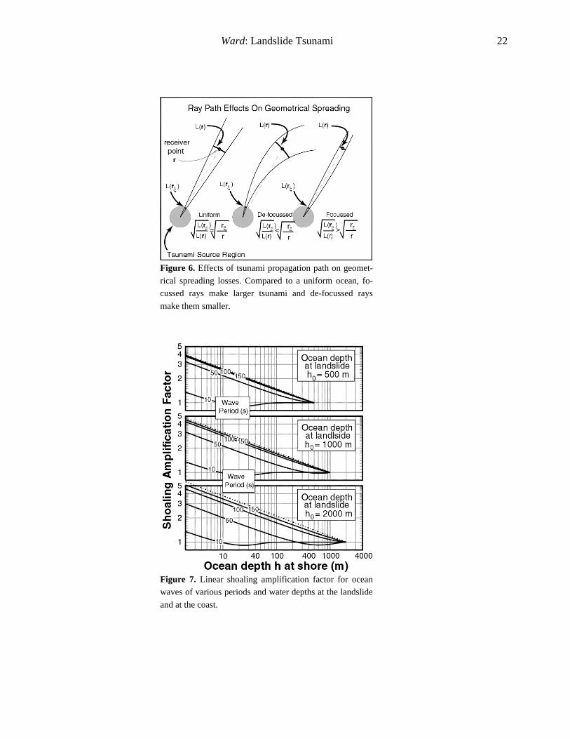
cally larger or smaller. Figure 6 cartoons typical
refraction cases and gives meaning to (15) as be-
ing the ratio of cross-sectional distances L(rξ) and
L(r) between adjacent rays measured near the
source at rξ and near the observation point at r.
Ward: Landslide Tsunami 9
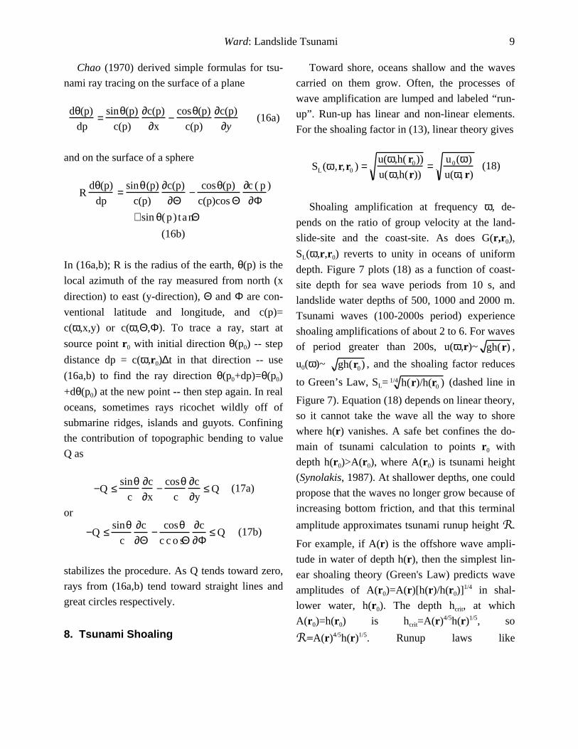
Chao (1970) derived simple formulas for tsu-
nami ray tracing on the surface of a plane
dθ(p)
dp=
sinθ(p)
c(p)
∂c(p)
∂x−
cosθ(p)
c(p)
∂c(p)
∂y (16a)
and on the surface of a sphere
Rdθ(p)
dp=
sinθ(p)
c(p)
∂c(p)
∂Θ−
cosθ(p)
c(p)cos Θ∂c ( p )
∂Φ+ sin θ(p) tanΘ
(16b)
In (16a,b); R is the radius of the earth, θ(p) is the
local azimuth of the ray measured from north (x
direction) to east (y-direction), Θ and Φ are con-
ventional latitude and longitude, and c(p)=
c(ω,x,y) or c(ω,Θ,Φ). To trace a ray, start at
source point r0 with initial direction θ(p0) -- step
distance dp = c(ω,r0)∆t in that direction -- use
(16a,b) to find the ray direction θ(p0+dp)=θ(p0)
+dθ(p0) at the new point -- then step again. In real
oceans, sometimes rays ricochet wildly off of
submarine ridges, islands and guyots. Confining
the contribution of topographic bending to value
Q as
−Q ≤sinθ
c
∂c
∂x−
cosθc
∂c
∂y≤ Q (17a)
or
−Q ≤sinθ
c
∂c
∂Θ−
cosθc c o sΘ
∂c
∂Φ≤ Q (17b)
stabilizes the procedure. As Q tends toward zero,
rays from (16a,b) tend toward straight lines and
great circles respectively.
8. Tsunami Shoaling
Toward shore, oceans shallow and the waves
carried on them grow. Often, the processes of
wave amplification are lumped and labeled “run-
up”. Run-up has linear and non-linear elements.
For the shoaling factor in (13), linear theory gives
SL(ω ,r,r0 ) =u(ω,h( r0))
u(ω,h(r))=
u0(ω)
u(ω, r) (18)
Shoaling amplification at frequency ω, de-
pends on the ratio of group velocity at the land-
slide-site and the coast-site. As does G(r,r0),
SL(ω,r,r0) reverts to unity in oceans of uniform
depth. Figure 7 plots (18) as a function of coast-
site depth for sea wave periods from 10 s, and
landslide water depths of 500, 1000 and 2000 m.
Tsunami waves (100-2000s period) experience
shoaling amplifications of about 2 to 6. For waves
of period greater than 200s, u(ω,r)~ gh(r) ,
u0(ω)~ gh(r0) , and the shoaling factor reduces
to Green’s Law, SL= h(r)/h(r0 )1/4 (dashed line in
Figure 7). Equation (18) depends on linear theory,
so it cannot take the wave all the way to shore
where h(r) vanishes. A safe bet confines the do-
main of tsunami calculation to points r0 with
depth h(r0)>A(r0), where A(r0) is tsunami height
(Synolakis, 1987). At shallower depths, one could
propose that the waves no longer grow because of
increasing bottom friction, and that this terminal
amplitude approximates tsunami runup height R.
For example, if A(r) is the offshore wave ampli-
tude in water of depth h(r), then the simplest lin-
ear shoaling theory (Green's Law) predicts wave
amplitudes of A(r0)=A(r)[h(r)/h(r0)]1/4 in shal-
lower water, h(r0). The depth hcrit, at which
A(r0)=h(r0) is hcrit=A(r)4/5h(r)1/5, so
R=A(r)4/5h(r)1/5. Runup laws like

Ward: Landslide Tsunami 10
[R/h(r)]=[A(r)/h(r)]4/5 appear to fit laboratory
observations of breaking and non-breaking waves
within a factor of two over a large range condi-
tions (Synolakis, 1987), although in real life, sel-
dom are circumstances so orderly (e.g Titov and
Synolakis, 1997).
9. Scenario Landslide Tsunami
Let's put the theory to task and compute tsu-
nami on the surface of a sphere from scenario
landslides. For this, I consider only direct waves.
If reflections and diffractions are neglected, for a
site to experience a tsunami, it must have an un-
obstructed view (along a ray path) of a part of the
landslide. To speed the calculation, I set Q=0 in
(17b) so that tsunami rays follow great circles. In
this case, the components in the geometrical
spreading factor (15) become L(r )=P(r ,r0)dφ,
L(r)=Rsin∆dφ, and P(r,r0)=R∆, so
G(r,r0) = G(∆) =∆
sin∆ (19)
where ∆ measures angular distance from the slide
to the observation point.
Nuuanu Slide, Hawaii.
Date: 2.7 Ma.
Moore et al. (1989, 1994) have mapped debris
fields of 68 spectacular landmasses that have bro-
ken off the crest of the Hawaii swell and slid into
neighboring deeps over the past 20 million years.
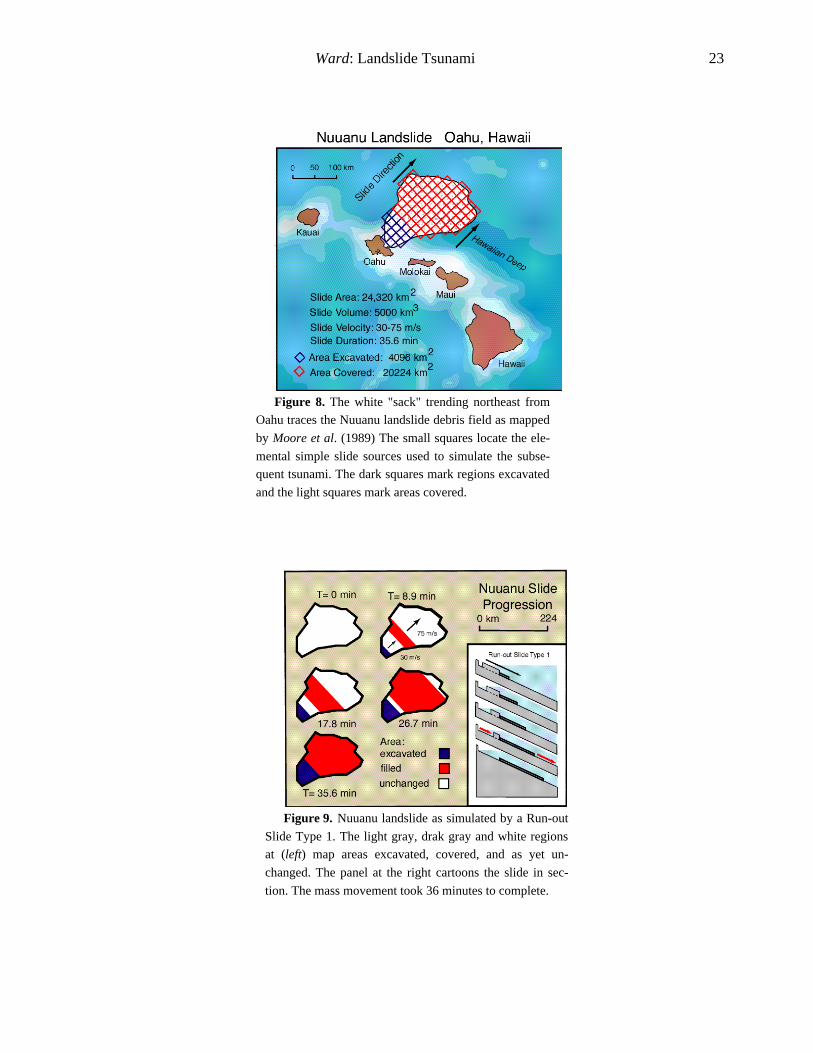
Chief among the group, with a volume of 5000
km3, is the Nuuanu landslide on Oahu’s north
shore (Figure 8). The slide scar covers 23,000
km2 in a teardrop-shape with the narrow end close
to the current shoreline. The slide ran out at high
speed as evidenced by large blocks that were car-
ried down into the Hawaiian Deep toward the
northeast and then rafted back uphill 350 meters
on the opposite slope. By analogy of a roller
coaster plying a frictionless track, the velocity of
the train at the base of a "dip" must be
vpeak= 2gH to carry it to a height H on the oppo-
site hill. If H=350 m, then the velocity of Nuuanu
slide at the base of the canyon must have been
about 80 m/s.
To simulate the Nuuanu slide, I use Run-out
Slide Model Type 1 that sequentially fires 95 in-
dividual simple slides, 16 km square, arrayed in
the grid shown in Figure 8. As modeled, the slide
has area of 24,320 km2 of which, 4,096 km2 was
excavated (darker area) and 20,224 km2 was cov-
ered (lighter area). The slide cut a 1220 m thick
slab (5000 km3) of material from the excavation
and deposited it in a 247 m thick layer over the
cover area. Certainly, part of the huge slab of ex-
cavated material extended above sea level before
the slide. To be conservative, the thickness of su-
baerial material should not be a tsunami produc-
ing part of the excavation. Accordingly, I set the
thickness of the excavated elements to the smaller
of the current water depth, or 1220 meters.
Figure 9 sketches the progression of the slide
in plan view and in section. As envisioned, a
1220 m thick block pulls away at the head of the
slide at vback= 30 m/s while the front of the block
disintegrates into a sheet 247 m thick and travels
down slope at vfront= 75 m/s. I drew vfront from the
roller coaster analogy. vback= 30 m/s equalizes
roughly the volume rates of excavation and fill. In
the cover area, ocean depth exceeds 2000 m and

Ward: Landslide Tsunami 11
tsunami travel faster than 140 m/s. Even at 75
m/s, the Nuuanu slide velocity substantially lags
the tsunami speed.
Figure 10 contours tsunami amplitudes at 18
minutes, 1 hour, 2.5 hours and 4.5 hours. In these
plots, blue and red color depressed and raised sur-
faces. The yellow dots and numbers sample the
wave height in meters. At 18 minutes, the slide,
bearly half complete, has set the ocean in full
turmoil. The fastest tsunami signal, a 40 m posi-
tive pulse, has already passed beyond the even-
tual extent of the slide. Interior to this forerunner,
atop the actively sliding zone, negative and posi-
tive waves greater than 100 m height gather. On
the coast of Oahu and Molokai, 50-60 m waves
have beached.
At 1 hour, mass movements have been com-
plete for 20 minutes and the ocean above the scar
begins to quiet. By now, 30-40 m waves have
struck Maui, Hawaii and Kauai. Other waves,
equally large, are still inbound. The directionally
of the radiation is evident in the strong waves
pushed slide-parallel, toward the northeast.
At 2 1/12 hours, dispersion has stretched the
tsunami into great sequence of waves spanning
1500 km front to back. The northeast travelling
pack peaks at 20 m height. Note that locations in
southwest quadrant have been saved the full force
of the wave thanks to the Hawaiian Islands dis-
rupting its passage.
At 4 1/2 hours, vanguards of the tsunami brush
the Aleutian Islands and the west coast of North
America. After crossing half of the Pacific Ocean,
waves 200 km offshore have managed to retain
10 m of amplitude. In their shoaling from 2000 m
depth, Figure 7 predicts growth by a factor of two
at least. I would say that the Nuuanu slide be-
stowed the Pacific Northwest coast with a 20 m
high wave.
Storegga Slide #1, Norway.
Date: 50,000-30,000y bp
The Pacific basin does not own bragging rights
to prodigious undersea landslides. In the Atlantic,
between 50,000 and 5,000 years ago, three large,
partly overlapping, landslides traversed a 500-
km-long submarine chute off the west coast of
Norway [Jansen, 1987]. Named Storegga #1, #2,
and #3, the slides had a combined volume of
5580 km3 -- comparable to the largest debris
fields mapped on the Hawaiian swell. The flared
head of the Storegga chute still can be seen taking
a noticeable bite out of the continental shelf at the
500 m contour (Figure 11, top left). The generally
rectangular slide scar runs northwest down the
continental slope to 3000 m depth and doglegs
250 to the north at its middle.
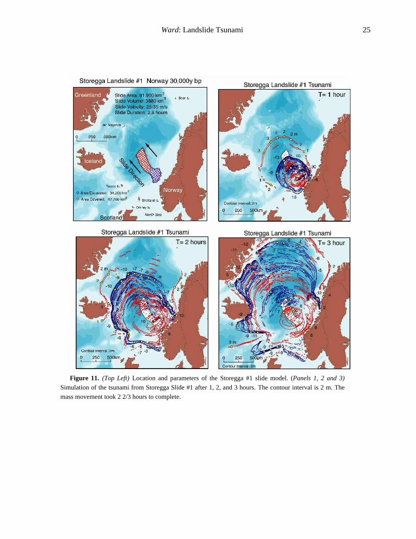
To simulate tsunami from the first, and big-
gest, Storegga slide, I follow the Nuuanu recipe
using Run-out Slide Type 1 and grid the scar with
91 simple slides, 30 x 30 km square (top left
panel of Figure 11). As modeled, the slide
spanned 81,900 km2 of which, 34,200 km2 was
excavated and 47,700 km2 was covered. The 3880
km3 slide volume [Jansen, 1987] was taken uni-
formly from the excavation (-113 m thickness)
and deposited uniformly over the distal fan (+81
m thickness). For the velocity of the Storegga
slide, no direct constraints exist. Compared to
Nuuanu, the depth of excavation was small, and
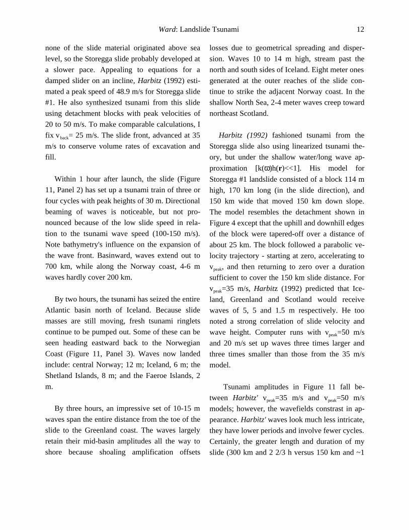
Ward: Landslide Tsunami 12
none of the slide material originated above sea
level, so the Storegga slide probably developed at
a slower pace. Appealing to equations for a
damped slider on an incline, Harbitz (1992) esti-
mated a peak speed of 48.9 m/s for Storegga slide
#1. He also synthesized tsunami from this slide
using detachment blocks with peak velocities of
20 to 50 m/s. To make comparable calculations, I
fix vback= 25 m/s. The slide front, advanced at 35
m/s to conserve volume rates of excavation and
fill.
Within 1 hour after launch, the slide (Figure
11, Panel 2) has set up a tsunami train of three or
four cycles with peak heights of 30 m. Directional
beaming of waves is noticeable, but not pro-
nounced because of the low slide speed in rela-
tion to the tsunami wave speed (100-150 m/s).
Note bathymetry's influence on the expansion of
the wave front. Basinward, waves extend out to
700 km, while along the Norway coast, 4-6 m
waves hardly cover 200 km.
By two hours, the tsunami has seized the entire
Atlantic basin north of Iceland. Because slide
masses are still moving, fresh tsunami ringlets
continue to be pumped out. Some of these can be
seen heading eastward back to the Norwegian
Coast (Figure 11, Panel 3). Waves now landed
include: central Norway; 12 m; Iceland, 6 m; the
Shetland Islands, 8 m; and the Faeroe Islands, 2
m.
By three hours, an impressive set of 10-15 m
waves span the entire distance from the toe of the
slide to the Greenland coast. The waves largely
retain their mid-basin amplitudes all the way to
shore because shoaling amplification offsets
losses due to geometrical spreading and disper-
sion. Waves 10 to 14 m high, stream past the
north and south sides of Iceland. Eight meter ones
generated at the outer reaches of the slide con-
tinue to strike the adjacent Norway coast. In the
shallow North Sea, 2-4 meter waves creep toward
northeast Scotland.
Harbitz (1992) fashioned tsunami from the
Storegga slide also using linearized tsunami the-
ory, but under the shallow water/long wave ap-
proximation [k(ω)h(r)<<1]. His model for
Storegga #1 landslide consisted of a block 114 m
high, 170 km long (in the slide direction), and
150 km wide that moved 150 km down slope.
The model resembles the detachment shown in
Figure 4 except that the uphill and downhill edges
of the block were tapered-off over a distance of
about 25 km. The block followed a parabolic ve-
locity trajectory - starting at zero, accelerating to
vpeak, and then returning to zero over a duration
sufficient to cover the 150 km slide distance. For
vpeak=35 m/s, Harbitz (1992) predicted that Ice-
land, Greenland and Scotland would receive
waves of 5, 5 and 1.5 m respectively. He too
noted a strong correlation of slide velocity and
wave height. Computer runs with vpeak=50 m/s
and 20 m/s set up waves three times larger and
three times smaller than those from the 35 m/s
model.
Tsunami amplitudes in Figure 11 fall be-
tween Harbitz' vpeak=35 m/s and vpeak=50 m/s
models; however, the wavefields constrast in ap-
pearance. Harbitz' waves look much less intricate,
they have lower periods and involve fewer cycles.
Certainly, the greater length and duration of my
slide (300 km and 2 2/3 h versus 150 km and ~1
Ward: Landslide Tsunami 13
1/2 h) must add extra persistence its waves. Har-
bitz' use of long wave theory may also contribute
to the difference in that this assumption makes
non-dispersive tsunami. Note too, that his tapered
block detachment model is decidedly smoother
and simpler in timing and shape than my run-out
slide. His block with 25 km tapers, traveling at 30
m/s will spread uplift at a point over TR=800 s
and exterminate waves of shorter period (see
equation 6). I suggest that slides onset far faster
than this, but in any case, to recognize and to un-
derstand the implications of their assumptions,
tsunami scientists must submit to "head to head"
comparisons of their models at every opportunity.
Agreeing to publish simple benchmark products,
such as the waves produced from basic slides like
those in Figure 2 or Figure 5, would be a step in
the right direction.
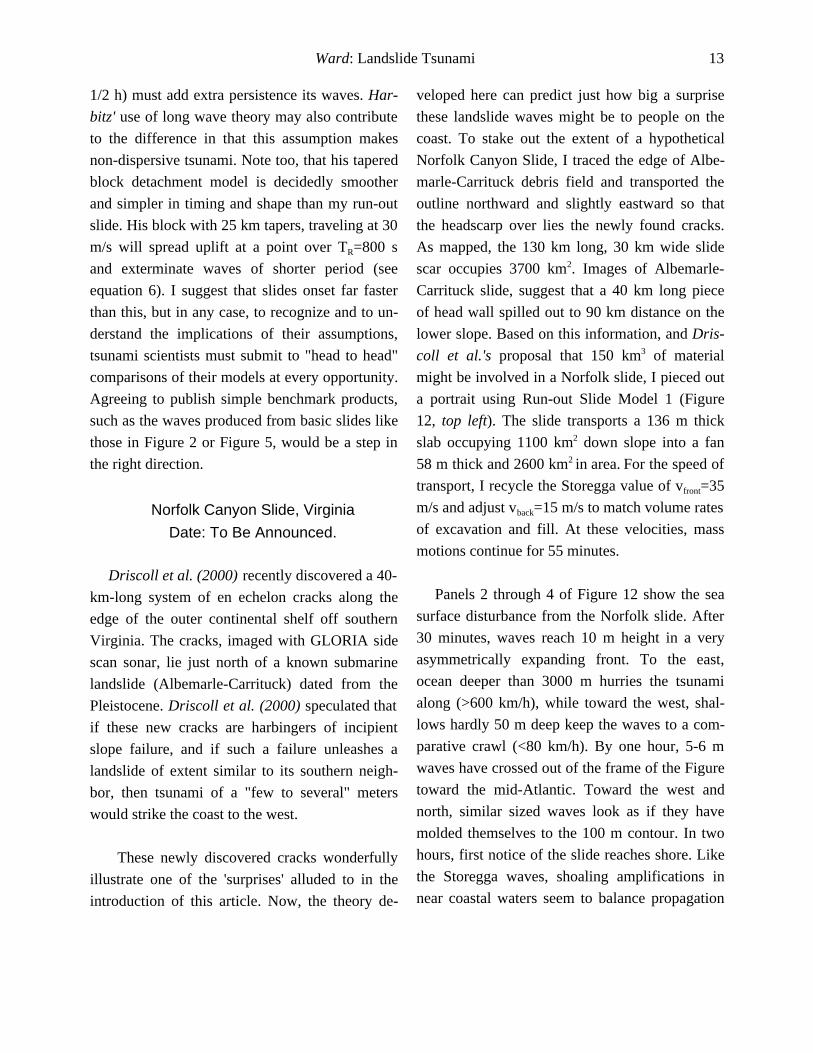
Norfolk Canyon Slide, Virginia
Date: To Be Announced.
Driscoll et al. (2000) recently discovered a 40-
km-long system of en echelon cracks along the
edge of the outer continental shelf off southern
Virginia. The cracks, imaged with GLORIA side
scan sonar, lie just north of a known submarine
landslide (Albemarle-Carrituck) dated from the
Pleistocene. Driscoll et al. (2000) speculated that
if these new cracks are harbingers of incipient
slope failure, and if such a failure unleashes a
landslide of extent similar to its southern neigh-
bor, then tsunami of a "few to several" meters
would strike the coast to the west.
These newly discovered cracks wonderfully
illustrate one of the 'surprises' alluded to in the
introduction of this article. Now, the theory de-
veloped here can predict just how big a surprise
these landslide waves might be to people on the
coast. To stake out the extent of a hypothetical
Norfolk Canyon Slide, I traced the edge of Albe-
marle-Carrituck debris field and transported the
outline northward and slightly eastward so that
the headscarp over lies the newly found cracks.
As mapped, the 130 km long, 30 km wide slide
scar occupies 3700 km2. Images of Albemarle-
Carrituck slide, suggest that a 40 km long piece
of head wall spilled out to 90 km distance on the
lower slope. Based on this information, and Dris-
coll et al.'s proposal that 150 km3 of material
might be involved in a Norfolk slide, I pieced out
a portrait using Run-out Slide Model 1 (Figure
12, top left). The slide transports a 136 m thick
slab occupying 1100 km2 down slope into a fan
58 m thick and 2600 km2 in area. For the speed of
transport, I recycle the Storegga value of vfront=35
m/s and adjust vback=15 m/s to match volume rates
of excavation and fill. At these velocities, mass
motions continue for 55 minutes.
Panels 2 through 4 of Figure 12 show the sea
surface disturbance from the Norfolk slide. After
30 minutes, waves reach 10 m height in a very
asymmetrically expanding front. To the east,
ocean deeper than 3000 m hurries the tsunami
along (>600 km/h), while toward the west, shal-
lows hardly 50 m deep keep the waves to a com-
parative crawl (<80 km/h). By one hour, 5-6 m
waves have crossed out of the frame of the Figure
toward the mid-Atlantic. Toward the west and
north, similar sized waves look as if they have
molded themselves to the 100 m contour. In two
hours, first notice of the slide reaches shore. Like
the Storegga waves, shoaling amplifications in
near coastal waters seem to balance propagation

Ward: Landslide Tsunami 14
losses in the final stages of travel. Although peak
amplitudes of 4-7 m spot the map, a typical visi-
tor along any beach from North Carolina to Long
Island would likely taste a 2-4 m wave after a
Norfolk Canyon submarine landslide.
10. Landslide Tsunami Hazard Estimation
As posed in the introduction, a quantitative as-
sessment of landslide tsunami hazard couples
tsunami theory with a census of potential land-
slide sources. This article marks a first step, and
even if many pieces are lacking, it is worthwhile
to lay out a route for the assessment. For this, I
build on Ward and Asphaug (2000) who recently
constructed probabilistic hazard tables for tsu-
nami from asteroid impacts.
The principal ingredients in a probabilistic
hazard assessment are:
(1) Maximum height Amax(ro, s) of tsunami gener-
ated atop landslides of given features
S=(ψ1,ψ2,ψ3…) [length, width, thickness, slide
velocity, etc.] in water of depth h(r0).
(2) Frequency of occurrence n(r0, s) of landslides
with features S at every offshore location ro.
(3) Tsunami amplitude loss in propagating from
the source location ro to coast location r.
(4) Tsunami amplitude gain due to shoaling on
approach to r.
(5) Statistical uncertainty of (1) to (4).
Some of these ingredients extract from the models
here. Others, are far from being in hand. Even so,
useful hazard estimates can be obtained when sta-
tistical distributions and empirical relations stand-
in. These approximations might contain just one
or two parameters that have to be found from ob-
servation or theory.
Element (1). Hazard estimation challenges tsu-
nami modelers to find the fewest landslide pa-
rameters S=(ψ1,ψ2,ψ3…) necessary to reasonably
characterize maximum tsunami amplitude
Amax(ro, s). As a start, Figure 3 points to
Amax(ro,V, v r) with slide volume V, slide speed vr,
and ocean depth h(r0), as chief players.
Element (2). The hardest nut to crack will be fix-
ing the joint frequency of landslide occurrence
n(r0, s). It might be made tractable if cleaved into
components. For example, suppose that experi-
ments find that slide velocity is (generally) inde-
pendent of slide volume. Then the function re-
duces to n(r0, s)=n(r0,V,vr,)=n(r0,V)P(r0,vr),
where n(r0,V) and P(r0,vr) specify the local rate of
landslides of volume V, and the probability that a
slide has velocity vr. I imagine P(r0,vr) being a
Gausssian with a mean and standard deviation
dependent on the seafloor slope at r0. Ideally, so-
nar recognizance would map the volume distribu-
tion of slides; however, in the absence of direct
information, a power law n(r0, V )= a(r0 )V− b(r0 )
may suffice. For landslide populations, the b-
value might be a universal scaling parameter as it
is for earthquakes. If so, the a(r0)-value then, rep-
resenting the total slide activity of a region, would
be the only parameter that needs to be extracted
from geological or geomorphological data.
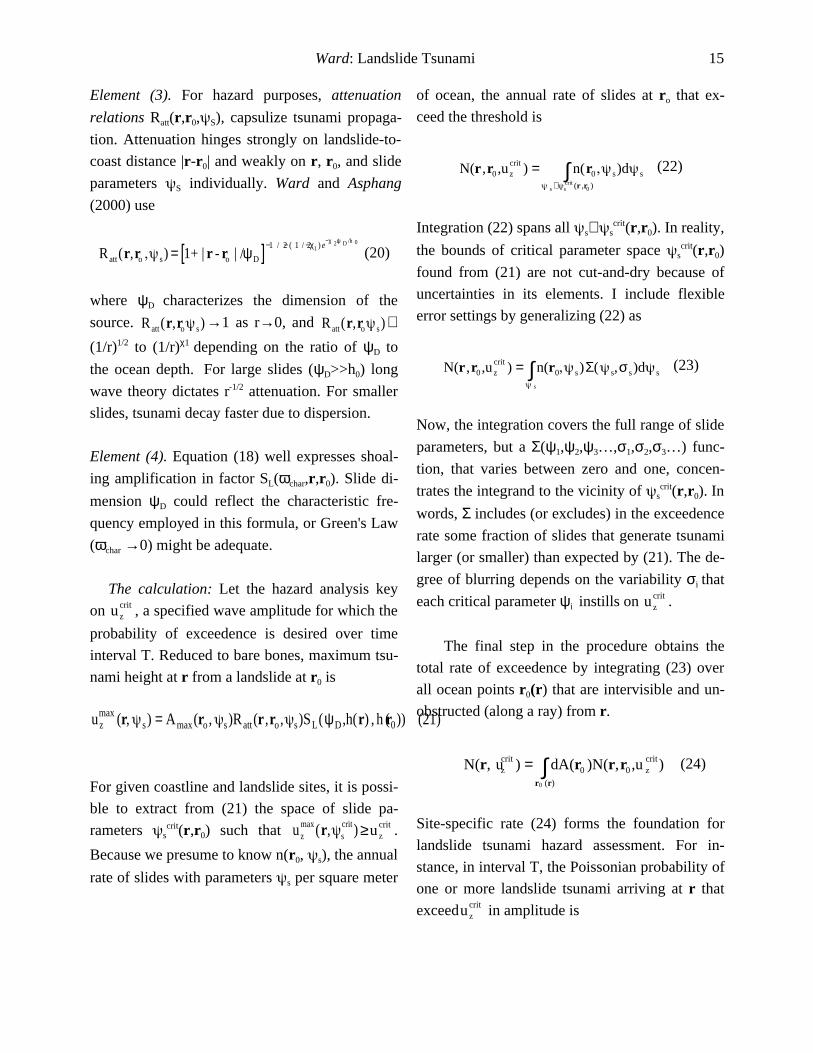
Ward: Landslide Tsunami 15
Element (3). For hazard purposes, attenuation
relations Ratt(r,r0, S), capsulize tsunami propaga-
tion. Attenuation hinges strongly on landslide-to-
coast distance |r-r0| and weakly on r, r0, and slide
parameters S individually. Ward and Asphang
(2000) use
R att(r,ro s) = 1+ | r - ro | /ψD[ ]−1 / 2− ( 1 / 2−χ1 ) e−χ 2ψ D /h 0
(20)
where ψD characterizes the dimension of the
source. R att(r,ro s)→1 as r→0, and R att(r,ro s)∝(1/r)1/2 to (1/r)χ1
depending on the ratio of ψD to
the ocean depth. For large slides (ψD>>h0) long
wave theory dictates r-1/2 attenuation. For smaller
slides, tsunami decay faster due to dispersion.
Element (4). Equation (18) well expresses shoal-
ing amplification in factor SL(ωchar,r,r0). Slide di-
mension ψD could reflect the characteristic fre-
quency employed in this formula, or Green's Law
(ωchar →0) might be adequate.
The calculation: Let the hazard analysis key
on u zcrit , a specified wave amplitude for which the
probability of exceedence is desired over time
interval T. Reduced to bare bones, maximum tsu-
nami height at r from a landslide at r0 is
uzmax (r, s) = Amax(ro , s)Ratt(r ,ro , s)SL(ψD ,h(r) , h (r0)) (21)
For given coastline and landslide sites, it is possi-
ble to extract from (21) the space of slide pa-
rameters scrit(r,r0) such that u z
max(r, scrit) ≥u z
crit .
Because we presume to know n(r0, s), the annual
rate of slides with parameters s per square meter
of ocean, the annual rate of slides at ro that ex-
ceed the threshold is
N(r ,r0 ,u zcrit ) = n(r0 s)d s
s ∈ scrit (r ,r0 )∫ (22)
Integration (22) spans all s∈ scrit(r,r0). In reality,
the bounds of critical parameter space scrit(r,r0)
found from (21) are not cut-and-dry because of
uncertainties in its elements. I include flexible
error settings by generalizing (22) as
N(r ,r0 ,u zcrit ) = n(r0 s)Σ( s,σ s)d s
s
∫ (23)
Now, the integration covers the full range of slide
parameters, but a Σ(ψ1,ψ2,ψ3…,σ1,σ2,σ3…) func-
tion, that varies between zero and one, concen-
trates the integrand to the vicinity of scrit(r,r0). In
words, Σ includes (or excludes) in the exceedence
rate some fraction of slides that generate tsunami
larger (or smaller) than expected by (21). The de-
gree of blurring depends on the variability σi that
each critical parameter ψi instills on u zcrit .
The final step in the procedure obtains the
total rate of exceedence by integrating (23) over
all ocean points r0(r) that are intervisible and un-
obstructed (along a ray) from r.
N(r, uzcrit ) = dA(r0 )N(r,r0 ,u z
crit)r0 (r)∫ (24)
Site-specific rate (24) forms the foundation for
landslide tsunami hazard assessment. For in-
stance, in interval T, the Poissonian probability of
one or more landslide tsunami arriving at r that
exceedu zcrit in amplitude is

Ward: Landslide Tsunami 16
P(r, T , uzcrit ) = 1− e− N(r ,u z
crit )T (25)
Poisson probabilities measure hazard simply, but
other more complex valuations employ the same
building blocks.
Given the potential magnitude of the risk (or
the unfounded fear of the risk) that tsunami land-
slide pose, I believe that a primary goal of geo-
physicists, geologists and oceanographers in the
next decade includes mapping landslide tsunami
probabilities along the coastlines of the world.
AcknowledgmentsI thank Costas Synolakis and Eric Geist for helpful reviews.
This work was partially supported by Southern California
Earthquake Center Award 662703. Institute of Geophysics
and Planetary Physics, University of California, Santa Cruz,
CA 95064. [email protected]
References
Chao, Y.Y., 1970. The theory of wave refraction in shoal-
ing water, including the effects of caustics and the
spherical earth, New York University, School of Engi-
neering and Science, University Heights New York,
10453.
Driscoll, N. W., J. K. Weissel, and J. A. Goff, 2000. Poten-
tial for large scale submarine slope failure and tsunami
generation along the U.S. mid-Atlantic coast, Geology,
28, 407-410.
Geist, E. 2000. Origin of the 17 July 1998 Papua New
Guinea tsunami: Earthquake or Landslide?, Seism. Res.
Lett., 71, 344-351.
Harbitz, C. B., 1992. Model simulations of tsunamis gener-
ated by the Storegga Slides, Marine Geology, 105, 1-
21.
Jansen, E., S. Befring, T. Bugge, T. Eidvin, H. Holtedahl,
and H. P. Sejrup, 1987. Large submarine slides on the
Norwegian continental margin; Sediments. transport
and timing, Marine Geology, 78, 77-107.
Moore, J. G., D. A. Clague, R. T. Holcomb, P.W. Lipman,
W. R. Normark, and M. E. Torresan, 1989. Prodigious
submarine landslides on the Hawaiian Ridge, J. Geo-
phys. Res., 94, 17,465-17,484.
Moore, J. G., W. R. Normark, and R. T. Holcomb, 1994.
Giant Hawaiian landslides, Ann. Rev. Earth and Planet.
Sci., 22, 119-124.
Synolakis, C. E., 1987, The runup of solitary waves, J.
Fluid Mech., 185, 523-545.
Tappin, D. R., et. al., 1999. Sediment slump likely caused
Papua New Guinea tsunami, EOS, 80, 329-340.
Titov, V. V. and C. E. Synolakis, 1997. Extreme inundation
flows during the Hokkaido-Nansei-Oki tsunami, Geo-
phys. Res. Lett., 24, 1315-1318.
Ward, S. N. and E. Asphaug, 2000. Asteroid Impact Tsu-
nami: A probabilistic hazard assessment, Icarus, 145,
64-78.
Ward, S. N., 2000. “Tsunamis” in The Encyclopedia of
Physical Science and Technology, ed. R. A. Meyers,
Academic Press, in press.
Steven N. Ward
Institute of Geophysics and Planetary Physics
University of California
Santa Cruz, CA 95064 USA
Ward: Landslide Tsunami 17
Figure 1. (top panel) Phase velocity c(ω) (solid lines) and
group velocity u(ω) (dashed lines) of tsunami waves on a
flat earth covered by oceans of 1, 2, 4 and 6 km depth.
(bottom panel) Wavelength associated with each wave
period. In general, tsunami generated from seabed distur-
bances in water of depth h, have wavelengths greater than
3h.
Ward: Landslide Tsunami 18
Figure 2. Tsunami produced by simple submarine slides. The
slide is 1-m thick and occurs over a 50 x 50 km area. The slide
starts to the left and moves to the right at speeds of 50, 100 and
250 m/s. Note the strong amplification of the wave in the slide
direction when the slide speed nearly equals the tsunami speed
of gh = 99 m/s. Small numbers in the upper right of each
panel are maximum and minimum wave heights.

Ward: Landslide Tsunami 19
Figure 3. Effects of slide velocity, slide dimension and
water depth on peak tsunami height. Slides that happen
too fast (right sides of boxes) or too slow (left sides of
boxes) are inefficient generators of tsunami. The stars
in the top left panel indicate the conditions in top, mid-
dle and bottom cases of Figure 2.

Ward: Landslide Tsunami 20
Figure 4. Under linear theory, complex landslides can be
produced by combining simple ones. Block, Run-out and
Sand Pile slides hint at the range of possibilities. The
Green's function approach permits more geologically real-
istic landslide behaviors than do many engineering-type
descriptions.
Ward: Landslide Tsunami 21
Figure 5. Tsunami generated from a 1 m thick de-
tachment block dragged 50 km at 100 m/s in a constant
depth ocean. The width (in the slide direction) of the
blocks are 6 km (top) and 25 km (bottom).
Ward: Landslide Tsunami 22
Figure 6. Effects of tsunami propagation path on geomet-
rical spreading losses. Compared to a uniform ocean, fo-
cussed rays make larger tsunami and de-focussed rays
make them smaller.
Figure 7. Linear shoaling amplification factor for ocean
waves of various periods and water depths at the landslide
and at the coast.
Ward: Landslide Tsunami 23
Figure 8. The white "sack" trending northeast from
Oahu traces the Nuuanu landslide debris field as mapped
by Moore et al. (1989) The small squares locate the ele-
mental simple slide sources used to simulate the subse-
quent tsunami. The dark squares mark regions excavated
and the light squares mark areas covered.
Figure 9. Nuuanu landslide as simulated by a Run-out
Slide Type 1. The light gray, drak gray and white regions
at (left) map areas excavated, covered, and as yet un-
changed. The panel at the right cartoons the slide in sec-
tion. The mass movement took 36 minutes to complete.

Ward: Landslide Tsunami 24
Figure 10. Simulation of the tsunami from the Nuuanu landslide. Times are 18 minutes, 1 hour, 2 1/2
hour and 4 1/2 hours. Contour intervals are 10 m, 5 m, 5 m and 2 m respectively.
Ward: Landslide Tsunami 25
Figure 11. (Top Left) Location and parameters of the Storegga #1 slide model. (Panels 1, 2 and 3)
Simulation of the tsunami from Storegga Slide #1 after 1, 2, and 3 hours. The contour interval is 2 m. The
mass movement took 2 2/3 hours to complete.

Ward: Landslide Tsunami 26
Figure 12. (Top Left) Location and parameters of a Norfolk Canyon Slide. Thirty-seven, 10 x10 km simple slides com-
prise this model. (Panels 2, 3 and 4) Tsunami after 1/2, 1, and 2 hours. Note how long it takes for the waves to traverse
the shallow continental shelf.
Ward: Landslide Tsunami 27
Top Related