


Languages
Pages
Legal


Investor Information Acquisition and Money Market Fund RiskRebalancing during the 2011-12 Eurozone Crisis*
Emily Gallagher† Lawrence Schmidt‡
University of Colorado Boulder Massachusetts Institute of Technology
Allan Timmermann§ Russ Wermers¶
University of California, San Diego University of Maryland at College Park
March 12, 2019
Abstract
We study investor redemptions and portfolio rebalancing decisions of prime money market mutualfunds (MMFs) during the Eurozone crisis. We find that sophisticated investors selectively acquire in-formation about MMFs’ risk exposures to Europe, which leads managers to withdraw funding frominformation-sensitive European issuers. That is, MMF managers, particularly those serving the mostsophisticated investors, selectively adjust their portfolio risk exposures to avoid information-sensitiveEuropean risks, while maintaining or increasing risk exposures to other regions. This mechanism helpsto explain the occurrence of selective “dry-ups” in debt markets where delegation is common and returnsto information production are usually low.
Key words: Money market funds, Eurozone crisis, financial fragility, endogenous information acqui-sition.
JEL: G01, G21, G23
*We thank Itay Goldstein and two anonymous referees for numerous constructive comments on the paper. We also thank partici-pants at the 2013 Workshop of the Dauphine-Amundi Asset Management Chair, the 2016 American Finance Association Meetings,the 2016 Midwest Finance Association Meetings, and seminar participants at Australian National University, Copenhagen Busi-ness School (FRIC 2017 conference on financial frictions), Northwestern University (Kellogg), Monash University, SouthwesternUniversity of Finance and Economics (Chengdu, China), University of Houston, and University of Melbourne. Finally, we aregrateful to Doug Diamond, Phil Dybvig, Maryam Farboodi, Gary Gorton, Bengt Holmstrom, Antoine Martin, and Zongyan Zhufor very helpful discussions and comments on the paper. The authors have received financial support from the Dauphine Chair inAsset Management, an initiative of Amundi and the University Paris-Dauphine, under the aegis of the Dauphine Foundation. Theviews expressed here are those of the authors only; as such, they do not represent those of any of the affiliated institutions or dataproviders.
†Finance Department, Leeds School of Business, 995 Regent Dr, Boulder, CO 80309. [email protected]‡Finance Group, Sloan School of Management, 100 Main St, Cambridge, MA 02142. [email protected]§Rady School of Management, 9500 Gilman Drive, La Jolla CA 92093. [email protected]¶Smith School of Business, 7621 Mowatt Ln, College Park, MD 20742. [email protected]

1 Introduction
Intermediated short-term debt markets play a key role in providing liquidity to firms and households.
Through intermediation, large volumes of near riskless, short-maturity debt contracts are regularly writ-
ten and rolled over by issuers, with minimal frictions and with little attention paid by financial markets. A
leading example of low-involvement intermediation is prime money market mutual funds (MMFs) which,
with assets totalling about $3 trillion at the end of 2018, are a major source of corporate debt funding,
especially for financial institutions.1
In normal times, short-term debt securities fluctuate little in value because their payoffs are near-certain
and rarely change with the arrival of new information. In such an “information insensitive” environment,
investors have very limited incentives to expend resources to monitor intermediaries’ investment strategies,
and, with low expected benefits, may rationally choose to engage in little to no information acquisition,
reducing the transaction costs and redundant acquisition of information about collateral quality.2 Likewise,
absent concerns about fundamental credit quality, strategic complementarities (i.e. concerns about negative
externalities from other investors’ actions) play little role in governing investors’ choices.3
In such a setting, a rapid “dry-up” of liquidity may develop as a result of information events which
cause investors to become concerned, almost overnight, about the value of the often opaque, hard-to-value,
pools of assets backing debt obligations. These concerns, in turn, may generate incentives for debt-holders
to acquire information about risk exposures and/or to worry about the potential adverse effects of other
investors’ redemptions. Specifically, in MMF markets, redemptions may ensue when investors choose to
scrutinize funds’ portfolio exposures more carefully, revise expectations about other investors’ actions, and,
if risks are perceived to be too high, redeem their shares. Under these circumstances, MMF shares become
information-sensitive and investor perceptions of MMFs’ risks are suddenly differentiated. Nevertheless,
even during a crisis, information acquisition may be selective, and available information incomplete. After
all, MMF payoffs are, by design, insensitive to most changes in market conditions. Moreover, private
information acquisition is costly and MMF portfolios are complex, containing many securities from global
1See https://www.ici.org/research/stats/mmf/mm_12_20_18.2See, e.g., Dang et al. (2017), Gorton (2017), Dang et al. (2015), Holmstrom (2015), and references therein.3For models of intermediation with strategic complementarities, see e.g., Diamond and Dybvig (1983); Goldstein and Pauzner
(2005). For applications to open-ended mutual funds, see, e.g., Chen et al. (2010); Schmidt et al. (2016); Goldstein et al. (2017).
1
issuers.4
Motivated by these ideas from prior theoretical models, this paper empirically documents a novel source
of fragility in short-term debt markets that is driven by such an incomplete information acquisition setting.
Selective or incomplete information acquisition by investors can prompt selective portfolio rebalancing by
intermediaries (i.e., MMF portfolio managers) by creating incentives to avoid holding only those securities
that are most impacted by the negative news signals at the onset of a crisis. To the extent that such rebalanc-
ing by portfolio managers suppresses their investors’ need to engage in subsequent information acquisition
and/or reduce strategic complementarities, rebalancing may prevent further redemptions. Thus, managers
may rationally exhibit an aversion to “headline risk” and avoid information-sensitive securities. In MMF
markets, where the benefits of maintaining exposures to comparatively riskier securities are quite low, even
small fluctuations in perceived risks can be associated with rapid dry-ups in funding for the issuers of such
securities.
To shed light on this mechanism, we study investor responses to initial portfolio risk and the subsequent
portfolio rebalancing by MMF managers during the 2011-12 Eurozone crisis, where a major concern for
investors was the geographic origin of the issuer of a particular security. At the time, numerous press reports
cited concerns from regulators and other market participants about the exposures of European banks to a
potential Greek default. These events increased the quantity/value of available information about individual
MMFs’ exposures to European default risk, relative to risks emanating from other regions, plausibly making
redemptions disproportionately sensitive to cross-sectional differences in MMFs’ European exposures.5
Since investors choose how much information, if any, to acquire about credit risk, we should expect
to see the largest amount of information acquisition and the largest flow responses to individual funds’
credit risks among investors with the greatest comparative advantage (i.e., lowest costs/highest benefits)
4Consistent with this hypothesis, Peter Crane (CEO of Crane Data, one of the two major data vendors for MMFs) noted in aninterview with the authors that shortly prior to the 2008 failure of Lehman Brothers (and a subsequent run on the MMF sector), “theReserve Primary Fund was posting its full portfolio on its website and updating it daily, so it showed all of that Lehman paper sittingthere. That didn’t stop all of the big institutional clients from leaving their cash there over the weekend [during which Lehmanfailed].” By this time, Lehman’s stock was already down 95% from its 52 week high and the Reserve Primary Fund – a large MMFthat “broke the buck” during the crisis – held more than 1% of its portfolio in Lehman’s short term debt.
5Such heterogeneity in redemption decisions contrasts with the more uniform redemptions from riskier MMFs that would beexpected following an increase in investor risk aversion alone or in the absence of information processing capacity constraints.Even if investors begin to acquire more information, most are unlikely to have the information processing infrastructure in place topermit efficient risk reallocation in bad times. As formalized by Hanson and Sunderam (2013), it takes time and resources to scaleup capacity to collect and process information. Thus, information acquisition, even by sophisticated investors, is likely selectiveand incomplete during stress episodes, as shown by the anecdotal evidence discussed in the prior footnote.
2

in acquiring and processing information. Also, more precise public information (i.e., a market-wide lower
marginal cost of gathering information) about European issuers’ changing default risks might make investors
better able to coordinate runs on individual MMFs with high European exposures. In both cases, MMF
managers who cater predominantly to highly sophisticated investors have the strongest incentives to quickly
move their portfolios away from these informationally-sensitive securities.6
Taking advantage of the rich detail available in MMF portfolio holdings reports starting November
2010, we provide empirical evidence consistent with MMF managers acting upon such incentives. To the
extent that a reduction in risk exposure to certain issuers is not replaced one-to-one with added exposure to
other issuers, such behavior may indeed have the effect of making MMF investors’ payoffs safer. However,
fragility may simply be pushed one link further down the chain by concentrating a reduction in financing on
a particular subset of issuers. As is well known, MMFs rapidly and dramatically cut exposures to European
issuers during the period of our study (see, e.g., Ivashina et al., 2015). We offer evidence that, controlling
for initial risk exposures, managers with the most attentive investors adjusted their portfolios away from
Eurozone credit risks by the largest amount. At the same time, MMF funding of issuers from outside
of Europe with comparable default probabilities remained stable or even increased throughout the period,
consistent with a selective focus on the part of fund investors and, in turn, fund managers.
We note that testing these ideas requires (i) accurate measures of fund-level credit risk, commensurate
with the real-time information available to sophisticated investors, and (ii) good proxies for (heterogeneous)
investor information acquisition and their processing capacity. To this end, we combine granular MMF
portfolio holdings data – the same information available to investors on a monthly basis as of the end of
2010 – with a data set of contemporaneous issuer default probabilities to calculate forward-looking, fund
and security-level credit risk measures that move with market conditions. These detailed data also enable
us to characterize fund manager portfolio rebalancing decisions throughout the crisis. Furthermore, we
use a unique, proprietary dataset of types of shareholders in each MMF shareclass to classify institutional
ownership (our proxy for low/high information acquisition costs) with more precision than in previous
6Schmidt et al. (2016) provide a model in which strategic complementarities are stronger in funds with a higher concentrationof sophisticated investors, so managers with better-informed investors may also have a stronger incentive to avoid informationsensitive securities. Further, when investors’ actions are strategic complements, investors have an incentive to “know what otherinvestors know” (Hellwig and Veldkamp, 2009) and acquire similar types of information. In our setting, given the media andregulatory focus on European exposures, it is most likely that investors would coordinate on acquiring more information aboutthese dimensions of portfolio risk, so these mechanisms potentially reinforce one another.
3

studies.7 We supplement this latter information with data logs containing a record of the number of times
investors view the fund filings on the SEC’s EDGAR website – a direct measure of investor acquisition of
the most readily available detailed information on MMFs.
Empirically, we find evidence consistent with the premise that sophisticated investors are the investors
most responsive to fund-level credit risk. Prime MMFs, especially those serving the most sophisticated
investor-types (“HiSOPH” funds), experience brisk outflows, amounting to roughly 10% of aggregate as-
sets, from June 8–July 5 of 2011.8 Moreover, outflows are sharpest among shareclasses with the highest
concentration of sophisticated investors and with higher credit risk at the onset of the crisis.9 In contrast,
we see little-to-no evidence of a differential response according to initial credit risk among shareclasses
owned by less sophisticated investors (“LoMiSOPH” funds). Our above-mentioned measure of investor in-
formation acquisition from the SEC EDGAR website also points to little information acquisition prior to
June 2011, followed by a substantial increase in information acquisition during the crisis. This increase
occurred almost exclusively among funds with a high concentration of sophisticated investors, suggesting
that more sophisticated investors were much more likely to have viewed the holdings information of indi-
vidual MMFs during the Eurozone crisis, motivating sophisticated investor outflows, at least in the absence
of risk-mitigating actions of MMF portfolio managers.
While sophisticated investors likely processed and incorporated holdings information into their redemp-
tion decisions, the data point to a selective focus on Europe. We find that European risk exposures are highly
predictive of redemption behavior within HiSOPH shareclasses relative to shareclasses with less sophisti-
cated ownership. In contrast, portfolio exposures outside of Europe are not associated with redemptions,
even in HiSOPH shareclasses, consistent with investors’ risk assessments narrowly focusing on the impact
of the Eurozone crisis on European issuers.
Turning to MMF managers’ responses, we provide multiple pieces of evidence consistent with an at-
7We consider a broad definition of “sophisticated accounts” as those in which natural persons represent a minority of ownershipinterest. By this definition, we estimate that 26% of self-designated “institutional” shareclasses of MMFs have less than 5%sophisticated ownership, while 16% of institutional classes have at least 95% sophisticated ownership, by dollar value.
8We choose July 5, 2011 as an endpoint because large outflows from prime funds ceased after that date, a well as to avoidcontaminating flows related to the Eurozone crisis with flows due to concerns about a potential breach of the U.S. debt ceiling inmid-to-late July 2011. For robustness, we also consider an alternative time range, similar to Chernenko and Sunderam (2014)–June1 to July 31, 2011–with qualitatively similar results.
9While we find that investor sophistication is a clear predictor of information acquisition during the crisis, having a higherinitial risk exposure, conditional on sophistication, does not predict higher information acquisition across funds at the onset of thecrisis.
4
tempt by managers of HiSOPH funds to make their portfolios less informationally sensitive. We demon-
strate that HiSOPH funds reduced the credit risk of their portfolios to a significantly higher degree, relative
to LoMiSOPH funds, per unit of initial European credit risk. Further, these reductions came completely from
efforts to rebalance away from European issuers. We find no evidence of similar reductions in exposure to
issuers outside of Europe, even when non-European initial exposures are high. To the contrary, HiSOPH
funds – funds more likely to be monitored by their investors – with initially high European exposures sub-
stitute more aggressively towards non-European exposures and, in the process, increase their non-European
credit risk level relative to their pre-crisis portfolios. These findings suggest that fund managers rebalanced,
not according to agnostic measures of issuer credit risk, but according to pressure from sophisticated in-
vestors on MMF managers to make portfolios less sensitive to events in Europe. Consistent with large
blockholders internalizing the costs of potential redemptions and being less selective in their information
acquisition efforts, we find that portfolio rebalancing away from Europe is more muted in funds with more
concentrated ownership (as proxied for by their average balance size).
We consider three alternative explanations for our findings. First, our rebalancing analysis compares
funds with similar ex-ante risk levels but different investors. A natural concern could be that HiSOPH
funds differ from their peers in terms of unobservable exposures to the Eurozone crisis, which might lead
them to reduce their European holdings more aggressively. However, we demonstrate that the relationship
between initial credit risk and observed increases in counterfactual credit risk is similar across HiSOPH
and LoMiSOPH funds, and that several observable measures of pre-crisis portfolio composition are similar
across groups, conditional on our initial risk measures. Second, similar to the evidence in Strahan and
Tanyeri (2015), the need to meet heavy redemptions may have led HiSOPH funds with greater European
exposures to pull back proportionally to their regional allocations, implying that our results, in part, might
be driven by outflows as opposed to a desire to reduce portfolio information sensitivity. However, results
are insensitive to various controls for redemptions, and we find similar differences between HiSOPH and
LoMiSOPH funds when we re-estimate the model for subsamples split on prior outflows.
A third alternative explanation involves regulations on the MMF investable universe. Perhaps, a dispro-
portionate fraction of European issuers, relative to issuers in other regions, simply drop below investment
grade and, thus, lose access to the heavily-regulated MMF sector. Such a scenario may explain managers’
5
focused withdrawals from this market. We find evidence counter to this simple “flight-to-quality” story;
that is, we observe very large reductions in the total value of issuance of short-term debt securities, and
reductions in maturities of new securities for essentially all European issuers – even those with low default
probabilities throughout the crisis. These reductions in total funding and maturities are larger for riskier
European issuers, consistent with the patterns documented for wholesale funding dry-ups in Perignon et al.
(2018) and Covitz et al. (2013). However, we find no similar reductions of funding on average, nor are
reductions in funding correlated with default risk, outside of Europe.
Our paper contributes to a recent literature studying sources of financial fragility in short-term funding
markets and, in particular, the 2011-12 Eurozone crisis.10 Chernenko and Sunderam (2014) find that, over
the summer of 2011, MMFs holding more Eurozone bank debt experience greater outflows. Correa et al.
(2013) find that, as MMFs reduced lending to European banks, U.S. branches of European banks reduce
lending to U.S. entities. Ivashina et al. (2015) make a similar argument, finding that European banks that
are more reliant on dollar-denominated funding from MMFs experience larger declines in their outstanding
dollar loans. The main focus of these papers is quite different from ours, however. They study how the
lending channel can generate credit supply shocks for firms outside of Europe. Conversely, we focus on
the information acquisition and monitoring behavior of investors with different sophistication levels and
the implications of this behavior for how managers restructure their portfolios following an initial credit
shock.11 Moreover, we propose new tests to plausibly identify this mechanism.
The remainder of the paper proceeds as follows. Section 2 contains a short background on MMFs
and the 2011-12 Eurozone crisis. Section 3 develops the hypotheses that we test in our empirical analysis.
Section 4 introduces our dataset, which is used to study investor redemptions and information acquisition
(Section 5) and fund portfolio risk reallocations (Section 6) during and after the Eurozone crisis. Section
7 compares the level of MMF funding available to individual issuers, both between and within regions.
Section 8 concludes.10Covitz, Liang, and Suarez (2013) study the asset-backed commercial paper (ABCP) market, while McCabe (2010), Kacper-
czyk and Schnabl (2013), Duygan-Bump et al. (2013), Strahan and Tanyeri (2015), and Schmidt et al. (2016) study investor behaviorand flows to MMFs around the Lehman crisis. Goldstein (2013) provides a survey of the empirical literature on bank runs.
11In other words, the primary focus of these earlier studies is on how changes in the total quantity of assets under management(which declined disproportionately for MMFs serving sophisticated investors and with high European credit risk exposures) affectthe total amount of lending to issuers in other regions.
6

2 Background: Money Market Funds and the Eurozone Crisis
MMFs are mutual funds that are widely used by U.S. corporations and individuals as a liquid cash in-
vestment. They invest exclusively in short-term debt securities, a “default-remote” contract designed to be
informationally insensitive. In normal times, investors may rationally choose to be inattentive to news about
the value of MMF portfolios, choosing to delegate the details of these investment decisions to a MMF man-
ager.12 On the asset side, they are an important provider of short-term financing to corporations, holding
16.6% of their aggregate portfolios in time deposits (e.g., bank CDs), 14.3% in commercial paper (CP),
26.9% in Treasury and Agency securities, 17.4% in repurchase agreements (repos), 13.8% in municipal
securities, and 11.0% in other investments at the end of 2010.13 Similar to a bank deposit account (but, in
actuality, an equity investment), shares in a MMF are designed to each have a constant value of $1, allowing
investment and redemption by investors without loss of principal (i.e., similar to a bank account).14 There
are three categories of money market funds: prime, government, and tax-exempt. Prime funds are the largest
category, the most flexible and riskiest of such funds.
MMFs must adhere to strict portfolio restrictions under SEC Rule 2a-7 of the Investment Company
Act of 1940. This provision, along with the ability to round prices to the nearest penny, allows MMFs
to maintain, almost always, the above-mentioned $1 per share net asset value (NAV); they may do so as
long as their mark-to-market portfolio values do not deviate by more than 50 bps from $1, under which
circumstance they would reprice NAV shares to “break the buck”. This feature of investors’ payoffs – that
those withdrawing from funds quickly may exit at the $1 NAV, leaving remaining investors to potentially
bear the costs of liquidating portfolio assets – creates a first-mover advantage and, in turn, makes investors’
redemption decisions strategic complements (Chen et al., 2010; Goldstein et al., 2017; Schmidt et al., 2016).
In 2010, the SEC adopted a set of amendments to Rule 2a-7 which mandated that funds file complete
portfolio holdings reports (Form N-MFP) within five days of month-end. These data facilitate a richer
analysis of fund portfolio risks than was possible during the 2008 crisis, which we exploit throughout this
paper.
12These features of short-term debt payoffs are discussed extensively in Gorton and Pennacchi (1990), DeMarzo et al. (2005),Holmstrom, 2015, Dang et al. (2017), and references therein.
13http://www.icifactbook.org/deployedfiles/FactBook/Site%20Properties/pdf/16_fb_table36.pdf14https://www.federalreserve.gov/releases/z1/current/accessible/l121.htm.
7
Investors responded to the Eurozone crisis with heavy redemptions from prime MMFs during June and
July of 2011. Citing their exposure to Greek debt, on June 15, 2011, Moody’s placed several French banks
on review for possible downgrade. Figure 1 shows that prime MMFs experienced outflows amounting to
roughly 10% of aggregate assets ($113 billion) from June 8–July 5 of 2011, and, at the same time, gov-
ernment MMFs experienced heavy inflows. After this period, however, the influence of the Eurozone crisis
on MMF flows is less clear. That is, later in July 2011, a second potential crisis appeared as Republicans
in the U.S. Congress demanded concessions in return for extending the federal debt ceiling. MMF flows
remained flat between mid-July until the debt ceiling deadline approached on August 2. Indeed, in late-July
and early-August of 2011, outflows from both prime and government MMFs rose sharply. To separate these
events, we focus on the period from June 8 through July 5 of 2011 when evaluating factors contributing to
rapid outflows from MMFs during the Eurozone crisis.
The Eurozone crisis continued long after flows began to slow from MMFs. Figure 2 shows average
5-year CDS premiums on banks in Europe, the U.S., and the Asia/Pacific region. Credit risk moved slowly
upward during June and July of 2011, accelerating in August of 2011. Credit risk remained high until
September of 2012, when the European Central Bank (ECB) announced that it would buy unlimited amounts
of the bonds of troubled Eurozone countries, thereby committing to be a lender of last resort.
Relative to issuers based in other regions, a disproportionate amount of public information was available
about the changing fortunes of European issuers during the period of our study. To demonstrate this, we
collect information from Bloomberg on the daily number of news articles written about each of the issuers
funded by prime funds and use this to construct indices of media attention by region, details of which are
provided in Appendix D. These indices, which we plot in Figure 3, track one another quite closely up until
May 2011, at which point media coverage of European issuers further increases, whereas media coverage on
issuers from other regions remains relatively flat. From July 2011 through the end of the year, the volume
of news articles on European issuers is roughly two to three times the average from 2010, and European
issuers continue to receive elevated levels of coverage relative to other regions, until the spring of 2012.
8

3 Hypothesis Development
In this section, we develop a set of hypotheses which we empirically test in the following sections. Our
first hypothesis is that, from the start of 2011 (shortly after holdings data first become available) until the
events of June 2011 described above, the MMF industry is in an information-insensitive state – meaning
that the expected benefit from incurring costs to distinguish the credit risk of individual MMFs is small. In
this state, more sophisticated MMF investors exhibit no greater responsiveness to changes in credit risk than
less sophisticated investors. Moreover, cross-sectional variation in credit risk does not predict investors’
subsequent information acquisition. Below, we test these predictions by considering the cross-sectional
correlation between investors’ redemptions (a signal of information acquisition) and MMF portfolio credit
risk, conditional on investor sophistication. We do so using data prior to the Eurozone crisis.
The onset of the Eurozone crisis is associated with sharply elevated default risk levels for the portfolio
holdings of some MMFs, increasing incentives of MMF investors to acquire information about funds’ risk
exposures. In this more information-sensitive regime, we expect investors, particularly larger, more sophis-
ticated institutional ones, to acquire more information. Investors, then, act on this information by retreating
selectively from funds for which fundamentals were revealed to be weak, leading to a reallocation of AUM
across funds. In this regime, the mechanisms discussed in Section 1 – costly information acquisition and
strategic complementarities – have several testable implications for the behavior of both investors and funds.
These implications are described next.
Starting with the investors, our second hypothesis is that investors with a comparative advantage at
monitoring (1) acquire/receive more information about individual funds’ risk exposures and (2) respond
more intensely to changes in funds’ perceived credit risks. Testing this hypothesis requires observable
proxies for monitoring costs, which we describe below. We expect these proxies to signal increased levels
of investor information acquisition, particularly for investors with low information acquisition costs. We
validate this expectation using web views of funds’ SEC filings.
In practice, information acquisition is costly, and investors likely differ in their likelihood of receiving
and/or capacity for processing information about portfolio risk. Since MMFs hold many heterogeneous as-
sets in their portfolios, risk assessment is complex and available information is often incomplete.15 When
15The evidence we present below (for example, the number of views of SEC filings in Figure 5) is consistent with unsophisticated
9
choosing between multiple types of signals to acquire, investors may find it beneficial to selectively ac-
quire information about a subset of assets (Kacperczyk et al., 2016) – most likely European assets in our
setting. Even those investors that do not actively pursue new information may still be exposed to certain
public signals during this period. We assume that investors were more likely to receive information about
European risks in MMFs’ portfolios, relative to risks emanating from other regions, and also that this type
of information may serve as a coordination signal. Hence, investors’ actions might be disproportionately
influenced by those risk exposures about which they are most aware. In particular, we expect to see larger
redemption responses to portfolio risks from European relative to other sources of risk, with the most sophis-
ticated investors responding comparatively more. We test these predictions by considering the correlation
between investor withdrawals and credit risk during the Eurozone crisis, separately by region and by investor
sophistication.
Turning to the behavior of fund managers, our third hypothesis is that incomplete information acquisi-
tion by investors will create manager incentives to selectively rebalance their portfolios. A key underlying
assumption is that changes in portfolio asset composition will change the information that investors are
likely to receive, whether from private information acquisition and/or from exogenous public signals. If
the signals associated with certain asset positions are perceived by managers as boosting the likelihood of
future redemptions, managers will reduce exposures to only the affected assets, even across sets of securities
with similar objective default probabilities. Thus, holding credit risk constant, we expect managers to more
aggressively rebalance away from assets for which the benefit/likelihood of acquiring information about
default risk is relatively high (and/or the cost is low). In addition, we expect these incentives to be strongest,
leading to relatively larger reductions in risk, in those funds that are most exposed to the initial information
event as well as in those funds catering to more sophisticated investors.16 Note that such rebalancing incen-
tives may exist irrespective of whether the underlying objective is to weaken complementarities or to avoid
private information acquisition on the part of sophisticated investors; we do not distinguish between these
investors (e.g., retail customers) receiving essentially no information about MMFs’ risk exposures during our sample period. Giventhe information insensitivity of MMF portfolio payoffs, we assume (and test below) that the decision by more sophisticated investors(e.g., institutional investors) regarding whether to disinvest will also be based upon incomplete information.
16Recall that, in the model of Schmidt et al. (2016), higher information processing capacity is associated with stronger com-plementarities. The argument that large institutional investors have a stronger incentive to withdraw from MMFs in response toincreases in credit risk is subject to the important caveat that very large blockholders better internalize the negative externalitiesassociated with their redemptions in response to news about credit risk (Chen et al., 2010) and refrain from doing so, which couldweaken these rebalancing incentives. We further discuss and empirically explore this point in section 6.2.
10

two potential mechanisms.
Managers can reduce the information sensitivity of their portfolios by rebalancing risk across regions
(i.e., if news about European issuers is more plentiful than news about Asia/Pacific issuers) and within
regions (i.e., if information about some European issuers is more readily available and/or valuable). We
expect that managers may choose to avoid the more information-sensitive issuers or security types, such as
those with lower expected recovery rates or longer maturities. We test these latter implications by studying
compositional changes of fund portfolios. We test all of the above predictions in Sections 6 and 7.
4 Data and Variables
Our empirical analysis relies on data merged from five sources, the union of which represents, to our knowl-
edge, the most comprehensive and complete empirical database studied to date on MMFs.
Our first data source consists of a complete record of the portfolio holdings of all prime MMFs at
each month-end in the 2011–2012 period. The SEC’s 2010 Amendments require each MMF, starting in
November 2010, to file Form N-MFP each month with the SEC. We obtain this detailed monthly portfolio-
level holdings information from SEC’s EDGAR data site. For each portfolio security, the fund must report
the name of the issuer, details about the issue (e.g., the type of security and whether it is collateralized), and
the security’s maturity. We categorize the holdings on Form N-MFP by the parent of the issuer.17 We assign
each parent firm to a particular region of the world, based on the parent firm’s headquarters. From this data
set, we calculate our main credit risk measures (discussed next) as well as measures of fund liquidity and
dollar exposures to European issuers during the crisis.
Second, to generate our credit risk measure, the “expected-loss-to-maturity” (ELM) of the fund’s port-
folio, we use default probabilities that match the time to maturity of each security in our N-MFP data. We
obtain default probabilities from the Risk Management Institute (RMI) of the National University of Singa-
pore. RMI generates forward-looking default probabilities for issuers on a daily basis for maturities of 1, 3,
6, 12, and 24 months ahead.18 We hand match firms in the RMI database with the list of parent companies
17Parent companies are often global firms that may need dollar funding from MMFs. For example, Honda Auto ReceivablesOwner Trust, which issues commercial paper in the U.S. to help finance auto loans to U.S. residents, is affiliated with Honda MotorCompany Ltd., which is its “parent.”
18These probabilities are generated using the reduced form forward intensity model of Duan, Sun, and Wang (2012). RMI coversaround 60,400 listed firms (some of which are no longer active) in 106 economies around the world and issues default probabilities
11

that issue debt to MMFs from our N-MFP data; this matching has a 90% success rate. For the remaining
10% of securities in N-MFP, we use other market quotes to arrive at estimated default probabilities (see
Appendix B). We calculate the expected-loss-to-maturity on a security as the issuer’s default probability
(maturity-matched to the security and then annualized) times the expected loss given default. Each security-
level risk estimate is then multiplied by its portfolio weight and summed across all securities in a fund’s
portfolio. ELM approximates the annualized expected loss on a fund’s portfolio.19 Appendix B details this
calculation and documents the necessary assumptions.
We use this framework to construct a counterfactual measure of credit risk (CELM) by applying current
default probabilities to fund portfolio holdings as of May 31, 2011. Then, by comparing ELM with CELM
after May 2011, we can determine whether a fund’s actual portfolio is more or less risky than its May
2011 portfolios would have been had the fund continued to hold the same securities with the same portfolio
weights as May 2011. This provides a timely measure of how a portfolio manager’s actions have altered the
fund’s risk profile since May 2011.
Figure 4 shows that ELM evolves with market conditions. This figure plots monthly asset-weighted
averages (across all prime MMFs) of three fund credit risk measures (LHS) and, for comparison, the
5-year CDS premium for the iTraxx European senior financial index (RHS). Fund credit risk measures
include ELM, its counterfactual (CELM), and the prime-to-government money market fund yield spread
(Yield spread). Yield spread is the most commonly used indicator of a prime fund’s credit risk. It is simple
to calculate, but the use of amortized cost accounting means that a fund’s yield spread can lag behind a
fund’s “true” credit risk. In Figure 4, average ELM and yield spread diverge by as much as 12 bps/year, and
yield spread appears to lag 2–3 months behind ELM throughout the crisis. In contrast, ELM and, especially,
CELM, appear to closely track the market’s perceived credit risk in European banks as measured by CDS
premiums.
for 34,000 firms. In fact, RMI publishes default probabilities for a number of firms which are important for our analysis, but forwhich CDS are not traded, notably for Canadian banks.
19To an extent, RMI’s default probabilities take into account the prospect of common shocks across firms. Our credit riskmeasure, ELM, does not, however, directly account for the extent of co-movement in default probabilities across firms held withinan individual fund’s portfolio. Correlated defaults with a portfolio could be of serious concern during those rare events when a largenumber of defaults occur simultaneously. Collins and Gallagher (2016) calculate the cost of “break the dollar insurance” (BDI),which accounts for correlation in credit risk across issuers but, unlike ELM, cannot be broken out into regional risk contributions.Borrowing their BDI measure, we find that it is highly correlated over time with ELM (ρ = 0.95 for the asset-weighted averagefund over time and ρ = 0.85 across individual funds). Moreover, we verify the robustness of our main results to using BDI insteadof ELM. See Appendix B and, in particular, Figures B1 and B2 for more details.
12

Third, we use a unique and novel database consisting of the proportion of assets, for each MMF share-
class, held by different categories of investors at the start of 2011. This proprietary data is compiled by the
Investment Company Institute (ICI) from fund transfer agents.20 A shortcoming of publicly available data
sets such as iMoneynet, is that so-called “institutional” shareclasses often are comprised of collective trusts
or omnibus accounts sold through brokers, which have large numbers of retail investors (also referred to as
“natural persons”). Thus, prior studies that treat all institutional shareclasses alike have missed a good deal
of the heterogeneity in the underlying investor base. As we show in Appendix Figure C1a, only about half
of the money in self-designated prime institutional shareclasses come from true institutions. Our preferred
measure of investor sophistication, SOPH, is the portion of “truly institutional” investors (i.e., accounts for
which natural persons do not represent the beneficial ownership interest) in a given fund or shareclass.21
Our maintained assumption is that these truly institutional investors are more sophisticated and face lower
costs of acquiring information.22
Fourth, we use a separate data source, iMoneyNet.com, to calculate investor flows to/from both indi-
vidual shareclasses and individual funds during the Eurozone crisis, along with several other explanatory
variables. Most notably, from daily iMoneyNet data, we obtain the dependent variable for cross-sectional
regressions explaining flows (FLOW ), which is measured as daily percentage changes in assets of each
shareclass during the crisis. From iMoneyNet, we also measure each class’s (log) total net assets (ASSET S),
historical flow variation (FLOWST D) and gross 7-day annualized yield (GY IELD).23
Finally, we use aggregate daily views of individual funds’ SEC Edgar filings as our proxy for investor
information acquisition, using files which track the number of hits on each page (URL) along with a blurred
20All statistical analyses were conducted using only high-level categorizations and de-identified data (this data is not publiclyavailable or for purchase). The data contains estimates of the number of accounts in each fund, from which we calculate each fund’saverage balance size. This variable is measured imperfectly, however, as brokers and 401(k) plans often pool their clients into one“omnibus” account which appear as one account despite containing a multitude of investors. Given this caveat, we use this variableonly as a control and in auxiliary analyses. We merge the RMI/N-MFP data set with ICI and iMoneyNet data based on EDGARidentifiers, CIK codes, and tickers.
21True institutional investors consist of nonfinancial corporations, financial corporations, nonprofit accounts, state/local gov-ernments, other intermediated funds (e.g., hedge funds and fund-of-fund mutual funds), and other institutional investors (e.g.,international organizations, unions, and cemeteries). See Appendix C for a more detailed discussion.
22We split all funds with at least one (self-designated) institutional shareclass into terciles based upon SOPH and use thebreakpoints from this procedure to sort all funds, including those with only retail shareclasses, into three categories. The breakpointsare at 13% and 57% of fund assets coming from sophisticated investors. While this procedure yields unequal numbers of fundswithin each group due to a large number of retail funds with near-zero sophistication, it creates more separation across funds, suchthat HiSOPH are markedly more sophisticated than remaining funds, on average–82% of the assets of the HiSOPH group areowned by sophisticated investors compared to only 14% of the assets of remaining funds (LoMiSOPH).
23FLOWST D is calculated as the (log) standard deviation of daily percentage changes in fund assets over the prior 3 months.This measure captures the historical liquidity needs of a fund’s investors (Gallagher and Collins, 2016; McCabe, 2010).
13

IP address of the user and a precise timestamp. For further details, see Appendix D.
Table 1 depicts rich heterogeneity in the characteristics of prime MMFs during the Eurozone crisis.24
While the median fund had outflows of just over 1% of its assets over the period of heavy redemptions in
June and early July of 2011, at the 10th percentile, outflows reached more than 15% of fund assets. The
number of EDGAR page views also rose relative to before the crisis, from 14.55 to 19.80, with an across-
fund standard deviation of 144.68 page views, implying substantial heterogeneity in investor attention as a
response to the crisis.
Next, we turn to measures of credit risk and rebalancing. The average fund had nearly 17 basis points
of credit risk over the 2011–2012 period, of which 10 bps came from European (“EU”) holdings and 7
bps came from non-European (“NotEU”) holdings. Counterfactual portfolios became much riskier over the
period, with average CELM of 24 bps, most of which (19 bps) could be attributed to European holdings.
The “pre” vs. “post” crisis comparison in the table suggests that actual MMF risk from Europe, ELM(EU),
fell marginally during the crisis, from 10.96 bps to 9.54 bps. Meanwhile, risk emanating outside of Europe
rose by about 3 bps. These differences, ELM−CELM, imply that substantial rebalancing occurred over the
crisis period. In fact, the average fund rebalanced 9.56 bps out of Europe and 1.61 bps into other regions.
As further evidence of rebalancing, the European share of credit risk from new securities (identified using
the CUSIP) fell from 77% to 56% as the crisis developed.
5 Investor Information Acquisition and Redemption Behavior
Focusing on the rapid outflows from prime MMFs that took place early on in the Eurozone crisis, this section
tests the prediction that selective information acquisition plays an important role in explaining investor
redemption choices following bad news signals.
5.1 Direct evidence on investor information acquisition
As argued in Section 3, MMF investors have limited incentives to actively acquire private information about
funds’ credit risk exposures in normal times. To test this prediction, we generate time series measures
of investor information acquisition by exploiting the availability of regulatory filings on the SEC EDGAR24These statistics are displayed at the fund portfolio level. Appendix Table A1 presents statistics for key variables used in our
fund flow regressions at the shareclass level.
14

website. Although investors can access information on fund portfolios from other sources, the information
available on the EDGAR website is standardized across funds and time during our period of study. It is also
updated regularly. Crucially, for certain key filings, we can unambiguously associate web traffic with the
specific filings of individual funds and then aggregate investors’ web traffic over time and across funds to get
a proxy for active information acquisition.25 Finally, the activity logs include a scrambled IP address, which
makes it possible to classify different page views according to the activity level of the user and exclude web
traffic that is unlikely to be associated with actual human interaction with the website.26
Figure 5 plots the total number of page views for different types of funds, expressed as a fraction of the
number of total accounts across all funds within each category, where we sort funds into three categories
–LoSOPH, MiSOPH, and HiSOPH– based on the fraction of AUM owned by sophisticated investors. We
express these monthly traffic levels as a rate per 10,000 investors. Further note that we graph the web
traffic series for the LoSOPH and MiSOPH funds on a separate axis, given that their activity measures
are substantially lower relative to HiSOPH funds, consistent with SOPH being a good proxy for investor
attentiveness; the average traffic levels for the three months prior to the start of the crisis–March through
May 2011–are 16.2, 1.2, and 0.66, for high, mid, and low sophistication-level funds, respectively.
Page views of HiSOPH funds’ filings increase sharply in the months of June and July 2011. In fact, the
spike at 189 views per 10,000 accounts is almost 12 times larger relative to the pre-period.27 Recall, much of
the news coverage about MMFs exposures occurred late in the month of June 2011. We observe non-trivial
increases in traffic levels for LoSOPH and MiSOPH funds, though the magnitudes are much smaller in both
absolute and percentage terms relative to the HiSOPH funds – consistent with true institutional investors
having a comparative advantage at information acquisition (as well as a larger benefit from their generally
larger positions). Information acquisition activity returns to pre-crisis levels from August 2011 onward.28
25We aggregate views of Forms N-MFP (holdings reports) and 497K (summary prospectuses), which make up a very large shareof total traffic on MMF’s EDGAR pages and can be uniquely linked with a single fund. Many of the other forms are filed at a higher(e.g., fund management company) level and contain less standardized information.
26A non-trivial fraction of EDGAR web traffic is related to automatic data collection algorithms, and the use of these algorithmshas increased over time to some extent. Following Loughran and Mcdonald (2014) and Lee et al., 2015, we apply a “no robot” filterwhich discards any IP addresses which view more than 50 unique CIKs (the SEC’s identifier) on a single day. Noting that there isa very strong time trend in the number of non-human views (these users are clearly identifiable from the timestamps in the data,see Loughran and Mcdonald (2014) ), we use the threshold they propose to rule out these sources of traffic. To the extent that theseviews are disproportionately coming from more sophisticated accounts, this likely works against us (since removing these "bot"views would understate the difference between traffic for HiSOPH funds relative to other funds).
27To the extent that, in addition to using Edgar, sophisticated investors are able to process holdings reports from fund manage-ment company websites, these measures of SEC page traffic are lower bound estimates of information acquisition.
28In unreported additional analysis, we aggregate the data in a slightly different way, classifying individual IP addresses into
15

These results are consistent with investors acquiring little-to-no information about credit risk in normal
times and support the view of financial crises as “information events” during which sophisticated investors
substantially increase information acquisition.29 To our knowledge, such direct evidence on changes in
information acquisition during a crisis is new to the literature.
5.2 Investor redemption behavior
Figure 6 provides preliminary evidence on the role of investor sophistication and credit exposure in explain-
ing redemptions from funds. It shows daily flows, aggregated across shareclasses, around the June 15, 2011
announcement that Moody’s had downgraded French bank credit ratings. The figure plots the log percentage
change in assets in the days around this announcement for four categories of shareclasses, cross-sorted by
ELM (fund credit risk) and investor sophistication, relative to assets under management as of May 31, 2011.
Class sophistication is measured by the portion of class assets held by sophisticated investors (SOPHc). Us-
ing the distribution of assets under management as of May 31, 2011, shareclasses are binned into low, mid,
and high terciles and, in regression specifications below, these categories are associated with the indicator
variables DLow,c, DMid,c, and DHigh,c, respectively.
Consistent with being in an information-insensitive regime in the days prior to the announcement,
cumulative flows to all four groups hovered close to zero and were in close alignment. Regardless of
investor sophistication, we observe no systematic difference in the redemptions of investors in funds with
high and low ELM prior to the June 2011 news events–which pushed MMFs into the spotlight.
From June 15th onward, “HiSOPH x HiELM” shareclasses experience large outflows during the two
weeks following the downgrade. On a cumulative basis, a very economically significant 12 percent of
assets were lost relative to peak AUM as of June 7th, whereas HiSOPH funds with lower risk exposures
do not experience withdrawals. In contrast, redemptions of less sophistication investors are similar for both
terciles based upon the level of activity on the EDGAR website. The spikes in activity are almost exclusively coming from the mostactive IP addresses on the site, consistent with information acquisition activities being concentrated among institutional investors,rather than retail investors. Performing a double sort on these (MMF and investor-level) classifications, we find that the increase inJune and July 2011 is predominantly driven by active EDGAR users looking at forms filed by HiSOPH funds.
29As further evidence, the small spike in page traffic for mid and high sophistication funds in February 2011 are most likelyrelated to an SEC press release from January 31, 2011 announcing the introduction of Form N-MFP. We are able to confirm thatmuch of the variation in SEC page views pre-dates the Eurozone crisis: many of the same investors who responded to the SEC’sJanuary 2011 press release also monitored fund N-MFP filings during the summer of 2011. In other words, there appears tobe a class of investors that followed the SEC announcement and learned about the information contained in the new form. Seehttps://www.sec.gov/news/press/2011/2011-32.html.
16

high and low ELM funds, consistent with earlier evidence of limited information acquisition among less
sophisticated investors. These patterns support the hypotheses in Section 3. However, this analysis does not
control for other potentially relevant investor or fund characteristics. Next, we conduct cross-sectional flow
regressions at the shareclass level.
In Section 3, we make predictions about differential redemption responses across investors with similar
MMF portfolios according to their ability (or incentive) to acquire information. Given our sample size, a
fully nonparametric matching procedure is impractical, so we approximate such an experiment through the
following regression specification, run at the shareclass level:
FLOWc =J
∑j∈{All},{EU},or{EU,NotEU}
RISKc, j ·[βLow, j ·DLow,c +βMid, j ·DMid,c +βHigh, j ·DHigh,c
]+X ′cγ + εc,
(1)
where shareclass-level variables, some of which vary only at the fund (portfolio) level, are denoted by “c”
subscripts and the j subscript refers to the geograpical source of credit risk (which can originate from “All”
regions, “EU, or “NotEU”).30 FLOWc, is the cumulative percentage change in class shares over the period
of heavy outflows, 6/7/2011–7/5/2011. Our benchmark portfolio credit risk measure, RISKc, j, is a fund’s
expected-loss-to-maturity (ELM f (c))31, which is identical across shareclasses within a fund.
Regression (1) also includes a number of class- and fund-level controls, Xc, including the logged total
net assets of the class and the fund (ASSET Sc and ASSET S f (c), respectively), the fund’s annualized gross
yield (GY IELD f (c)), the logged historical investor flow variation (FLOWST Dc), the share of fund assets not
maturing during the month nor invested in Treasury/Agency securities (ILLIQUIDITYf (c)), sophistication
category dummies as well as a continuous measure of class sophistication (SOPHc), the log of the average
balance size for the fund (BALSIZE f (c)), and an indicator for whether the class is designated as “institu-
tional” in the fund’s prospectus (INSTc). All independent variables are measured at the beginning of period
over which FLOWc is measured. To reduce the impact of outliers in flows (which tend to be driven by small
shareclasses), we winsorize flows at the 2nd and 98th percentiles and note that results are similar at other
30To economize on notation in equation (1), we mark all variables with a c subscript. In the text below, we identify variablesthat only vary at the fund-level with the subscript f (c), where f (c) captures the known mapping from shareclass to fund indices.
31In these flow-risk regressions, ELM f (c) is winsorized at the 98th percentile across security-level holdings before aggregationto the fund-level. The next section describes this process in more detail (see footnote 38). Winsorization is performed here to beconsistent with that later analysis. Results are similar with the un-winsorized ELM f (c) measure.
17

thresholds. All standard errors are clustered at the fund level.32
Table (2) summarizes the coefficients of interest from Equation 1 for different specifications and time
periods. Columns (1)–(3) estimate a monthly panel regression relating monthly flows with lagged fund
and investor characteristics using data for the four months prior to the crisis, where we also include time
fixed effects. In column (1) we interact total ELM with our sophistication indicators. Column (2) uses the
contribution to ELM from European (“EU”) issuers only. Column (3) estimates a bivariate specification
which allows for different coefficients on the contribution to fund ELM from European and non-European
(“NotEU”) issuers. In all three columns, we find a low R2 and small and statistically insignificant coefficients
on these credit risk measures, consistent with investors reacting very little to fluctuations in credit risk in
normal times. The bottom of the table includes p-values for a test of equal flow sensitivity of HiSOPH and
LoSOPH shareclasses to variation in credit risk, i.e., βLow,All = β High,All in columns (1), (4), (5), and (8) and
βLow,EU = β High,EU otherwise. We fail to reject this hypothesis in the pre-period. Our finding in column (3)
is consistent with Chernenko and Sunderam (2014), who find that European exposures do not predict flows,
controlling for yield.
The remaining columns (4)-(10) estimate the same specification using cumulative outflows during the
crisis period as the dependent variable. Here, notable differences begin to emerge depending on investor
sophistication. Columns (4)–(5) estimate Equation (1) using overall ELM as the credit risk measure without
and with controls, respectively. In both cases, coefficients are decreasing in investor sophistication, and
only βHigh is significant at the 95% level (we omit the second subscript since there is a single category).
This is consistent with our hypothesis, suggesting that investors who have a stronger incentive to acquire
information are more responsive to cross-sectional differences in funds’ credit risk exposures. Including
fund controls, we see a modest increase in the predictive power of the specification and a modest reduction
in the magnitude of βHigh. The estimated magnitude of βHigh in column (5) is nontrivial: it suggest that
predicted outflows from HiSOPH shareclasses would be about 4.0 percentage points larger (18 × 0.22) if its
fund’s ELM is at the 90th percentile relative to a fund with an ELM at the 10th percentile (see Table A1).
This effect is substantial relative to the change in aggregate assets under management for prime institutional
32Our analysis winsorizes at the 2nd and 98th percentile to manage the small fund denominator problem (i.e., flows will be morevolatile as a percentage of assets for smaller funds). To explore the robustness of our findings, we re-calculated the flow regressionsin Table (2) using winsorization at the 1st and 99th percentiles. While the associated tests are marginally less powerful due to theslightly greater influence of outliers, all but one of the columns maintain statistical significance.
18
shareclasses (-9%, see Figure 1).
Column (6) repeats the analysis using only the contribution to ELM from European issuers, discarding
any credit risk emanating from other regions. The estimate of βHigh increases and is highly significant,
whereas coefficients for other shareclasses (βLow and βMid) are small and insignificant. Moreover, the dif-
ference between βLow and βHigh is highly significant. We observe a slight increase in the R2 despite the fact
that our predictor variable ignores some sources of risk; at about 14 bps (see Table A1), the 90-10 spread for
European credit risk is non-trivial. It implies that a HiSOPH shareclass in a fund with European exposure at
the 90th percentile would receive outflows during the crisis period that are about 4.5 percentage points (of
assets) larger relative to a HiSOPH shareclass in a fund at the 10th percentile of European exposure. The
magnitudes of these effects are roughly on par with those in Chernenko and Sunderam (2014).
Column (7) estimates a bivariate specification which includes both European and non-European ELM.
As before, βHigh,EU is virtually unchanged and highly significant whereas the coefficient on not-Europe is
insignificant. These highly asymmetric responses to a credit risk measure, which is directly comparable
across regions, suggest that European risk was viewed by investors as being different, in the sense that
equivalent risks emanating from other regions were not associated with investor redemptions. Our results
point to a more nuanced response to the crisis than one that can be explained by a simple story in which
“EU securities were more risky and sophisticated investors ran on the riskiest funds.”33 Moreover, we
find evidence of selectivity among highly sophisticated investors. These results, coupled with qualitative
evidence of media coverage centered on MMFs’ European exposures in June-July 2011, suggest that fund
managers–especially those with sophisticated clients–had a disproportionate incentive to rebalance away
from European risks, which we investigate in the next section.
In interpreting the above findings, one must be wary of unobservable factors. An identification concern
would arise, for example, if, after controlling for the European ELM, HiSOPH funds differ from other funds
in terms of their exposures to unobserved elements of the Eurozone crisis that worsen over time. To partially
address this concern, in columns (8)–(10) we re-estimate the specifications from columns (5)–(7) using the
33Chernenko and Sunderam (2014) show that the fraction of AUM in European securities predicts outflows from sophisticatedinvestors, even after controlling for yield. Such a result could reflect the fact that, during this period, Eurozone exposure was abetter proxy for overall credit risk relative to the (backward-looking) yield measure. As such, while their empirical results areconsistent with selectivity, this finding does not speak to selectivity of investors’ redemption behavior per se. In contrast, our riskmeasures are constructed to have units (bp of credit risk) that allow for a direct comparison across regions–i.e., if investors wereequally responsive to European and non-European credit risks, we would expect βHigh,EU = β High,NotEU .
19

counterfactual expected-loss-to-maturity (CELM9/2011f ) in place of ELM f . This alternative measure captures
a fund’s credit risk as of 9/31/2011, had the fund continued to hold the same portfolio it held as of 5/31/2011,
just before the Eurozone crisis worsened. We choose 09/30/2011 because the Eurozone crisis had grown
acutely worse by this date (see Figure 2). Results are qualitatively similar to those based on ELM and are
highly statistically significant, though magnitudes are smaller (which is expected because the distribution of
CELM has more dispersion relative to ELM).34 Sophisticated investors appear to have redeemed more from
funds that were on a trajectory to have the highest expected losses during a prolonged Eurozone crisis.35
There is no evidence of a similar perspicaciousness with respect to impending risk from other regions.
6 Regional Portfolio Risk Rebalancing
The flow regressions in Table 2 suggest that sophisticated investors acquired information about and pre-
dominantly withdrew from funds with higher levels of credit risk. Further, these investors appear to have
selectively monitored risk attributable to investments in Europe, compared to other regions. This section
studies the portfolio rebalancing responses of fund managers in the wake of the outflows, and the extent to
which such rebalancing differed for funds that predominantly catered to sophisticated investors.
6.1 Rebalancing regressions
We evaluate the short-, medium-, and long-run influences of investor flows on fund managers’ (re-)allocation
decisions using the following cross-sectional regression at the fund-level:
REBALANCING f ,t = αt + ∑k∈Low,Mid,High
Dk f
[βktELM(EU) f +ωktELM(NotEU) f
]+X ′f ,tγt + ε f ,t , (2)
where the summation is over the three investor sophistication categories, k, defined at the fund-level as
discussed in Section 4 according to our estimate of SOPH f as of May 2011. Since, in aggregate, MMFs
34In Appendix Table A2, we estimate similar specifications which use the EDGAR page view data at the fund-level to form analternative proxy for the intensity of investor information acquisition based on the ratio of the number of page views in the monthsprior to June 2011 to the number of accounts in each MMF. We find very similar results to those from Table 2 when sorting onthis alternative measure of sophistication, despite it being generated from very different information. Again, investors who monitorfund websites are more responsive to credit risk, but their responses are selectively focused on European securities.
35This result does not, of course, imply that the most sophisticated investors necessarily anticipated the unfolding of the crisis.Rather, it suggests that these investors were able to identify funds with the greatest exposure to issuers that were most likely to beadversely affected if, as turned out to be the case, the Eurozone crisis continued to escalate.
20

experienced heavy redemptions only at the onset of the Eurozone crisis, and since the crisis endured long
after redemptions moderated, we can track the responses of fund managers over time. For instance, in the
short run, we might expect fund managers to have fewer opportunities to address the factors driving outflows
from their funds as they simply try to meet redemptions by offloading their most liquid assets.36
Our preferred rebalancing measure is ELM f ,t−CELM f ,t , the actual contribution of a region to a fund’s
credit risk (ELM f ,t) on a given date minus the counterfactual contribution (CELM f ,t), both measures poten-
tially being region-specific (we omit this notation for simplicity). By constructing counterfactual portfolios,
we can adjust for the credit risk a fund would have had on a given date had the manager elected to do nothing,
effectively holding an unchanged set of securities. Thus, the dependent variable captures a fund manager’s
efforts since May to actively increase (+) or reduce (-) the fund’s credit risk relative to the pre-crisis baseline
portfolio on May 31, 2011. We take snapshots of this variable at the end of each month during the Eurozone
crisis. Our vector of controls, X f ,t , includes the fund-level versions of the same controls considered in the
flow regression above in addition to the reduction in assets under management, if any, experienced by each
fund during the onset of the crisis, OUT FLOWf . Credit risk changes substantially throughout the crisis, so
we allow these coefficients to vary across calendar months then present averages over various periods.37
The key explanatory variable of interest in (2) is the interaction between ELM(EU) f , which measures
the initial level of European exposure of a fund’s portfolio prior to the start of the crisis, and dummies
Dk f which, as above, separate funds into three categories based on the fraction of assets under manage-
ment owned by sophisticated investors, with DHigh, f indicating the tercile with the highest concentration
of sophisticated investors. Our baseline specification separates risk into components associated with Euro-
pean and non-European exposures, constructed as the average of each fund’s regional ELM measures from
January through May 2011.
We apply two simple adjustments to the data before estimation. First, since we are interested in how
variation in initial European exposures correlates with rebalancing, we exclude funds that have essentially
no (ELM(EU) f < 2 bp) pre-crisis European exposure to potentially rebalance out of. Second, we observe
that, as the crisis develops, a small number of funds have substantial initial exposures to a small subset of
issuers (in particular, the Belgian bank Dexia) that experience dramatic increases in their default probabil-
36Strahan and Tanyeri (2015) find that funds with greater outflows during the 2008 MMF crisis became temporarily riskier asmanagers fed redemptions with the safest and most liquid assets.
37Similar results obtain from restricted models which impose constant coefficients over longer periods, e.g., calendar quarters.
21

ities starting in October 2011. These cases induce a handful of outliers in our credit risk and rebalancing
measures. To ensure that our conclusions are not influenced by a small number of pre-existing positions
subject to out-sized increases in default probabilities (essentially all of these positions had been eliminated
before October), we adopt a winsorization approach.38
The βkt , coefficients compare rebalancing activity of fund managers who had investors with similar
information acquisition costs (as proxied for investor sophistication measure) but different European ex-
posures. For instance, βHigh,t characterizes the change in expected rebalancing during the crisis (in basis
points) of a HiSOPH f manager in response to a one bp change in initial European risk exposure. Since
this coefficient is estimated in cross-sectional regressions, it is identified via differences in initial portfolio
composition across HiSOPH f funds.
An assumption underlying this setup is that differences in initial portfolio exposures are associated
with comparable differences in counterfactual exposures. In other words, initial differences in credit risk are
good proxies for increases in future portfolio risk, holding fixed the portfolio over time, and these differences
are comparable across HiSOPH and LoMiSOPH funds. This is essentially a “parallel trends” assumption
because it allows us to exploit differences in initial exposures that are comparable across sophistication bins.
Under these conditions, we would expect similar rebalancing patterns per unit of initial exposure if there is
little or no cross-sectional variation in investors’ information processing capacity.
Table 3 presents a formal test for this assumption – namely that differences in initial credit risk pre-
dict similar changes in portfolio risk exposures for HiSOPH versus LoMiSOPH funds. Specifically, we
test whether the coefficients on the linear projection of CELM f ,t , as well as its breakdown into regional sub-
components CELM(EU) f ,t and CELM(NotEU) f ,t , per unit of initial credit risk are comparable across funds
with different categories of investor sophistication. Columns (1)–(3) present averages of the monthly coef-
38Specifically, for each month in our sample, we compute the distribution of security-level ELM, where we weight holdingsaccording to their market values in the aggregate money market portfolios. We, then, winsorize security-level ELM at the asset-weighted 98th percentile, then compute ELM f ,t as asset-weighted average of the winsorized security-level measures. (We do notwinsorize below since the distribution is naturally bounded below by zero.) We follow an analogous procedure for CELM f ,t . Thisapproach has the advantages that it (a) applies the identical contribution to credit risk for two funds that hold the same securityat the same time and (b) makes the ELM measures additive across regions, which would not be the case if we computed fund-level measures first, then winsorized afterwards. We obtain similar results with higher and lower thresholds. For example, whenwe winsorize instead at the 99th percentile, we obtain modestly larger estimates for the rebalancing effects. For the most part,this happens because HighSoph funds had slightly higher average initial exposures to a couple of these distressed issuers, whichincreases the CELM coefficients a little more relative to our preferred specification with 98% winsorization. At the same time, ELM– CELM coefficients increase even more relative to our baseline estimates because HighSoph funds (like all others) eliminated theirpre-existing exposures to them. Accordingly, we prefer the more conservative approach because we do not want our results to beunduly influenced by modest differences between funds’ initial exposures to these issuers.
22

ficients from a specification identical to Equation (2) which uses total fund risk, CELM f ,t , as the dependent
variable. Different rows correspond to averages computed over different subperiods (roughly quarterly),
where the “Pre-crisis” period ranges from January through April 2011 (well before the downgrades of major
European banks), “Post-crisis” denotes the 12-month period from 2011Q4–2012Q3 when fund redemptions
had slowed but global credit risk was elevated, and different columns are associated with different sophisti-
cation groups.
While the coefficients in columns (1)–(2) exhibit non-trivial time-series variation, increasing substan-
tially relative to the pre-crisis period, the differences across investor sophistication bins in column (3) are
always statistically insignificant. This finding confirms our parallel trends assumption. Columns (4)–(6)
and (7)–(9) report the same coefficients for CELM(EU) f ,t and CELM(NotEU) f ,t , respectively. Results are
similar for EU exposures. Unsurprisingly, initial EU exposures are relatively uncorrelated with changes in
CELM outside of Europe, given that we are already conditioning on initial non-EU exposures. Point esti-
mates are weakly negative, but generally insignificant.39 The last row repeats this exercise, with all controls
dropped except for indicators for the sophistication categories. This more parsimonious specification further
supports our parallel trends assumption.
6.2 Investor information acquisition costs and fund risk rebalancing
Having established empirical support for our parallel trends assumption, we next present our main rebal-
ancing results. Panel A of Table 4 is structured as in the previous table, except that the dependent variables
are [ELM f ,t −CELM f ,t ], [ELM(EU) f ,t −CELM(EU) f ,t ], and [ELM(NotEU) f ,t −CELM(NotEU) f ,t ], re-
spectively. In the period prior to the crisis, differences between the βLow,t , βMid,t , and βHigh,t coefficients
are quantitatively small and statistically indistinguishable from one another, both overall and across regions,
suggesting that the average pre-period exposures are unrelated to pre-crisis trends in the accumulation of
credit risk.
Even in the very short run, fund managers with initially high levels of European credit risk exposures
began to reduce overall portfolio risk. The point estimates for 2011Q3, though far from trivial, are relatively
modest in magnitude relative to later periods and statistically indistinguishable between HiSOPH and other
39We present the coefficients on credit risk from outside of Europe (ωkt ) in Appendix Table A4. Again, we observe that initialnon-European exposures predict increases in counterfactual portfolio risk, consistent with the rise in global credit risk observed inFigure 2, and differences in ωkt across fund sophistication terciles are insignificant.
23
funds. Short-run efforts to reduce portfolio risk were likely impeded by the need to meet redemptions with
sales of more liquid securities, making it challenging initially to reduce risk. This channel may have been
more important for HiSOPH funds since they received above-average levels of redemptions during the crisis.
Focusing on the HiSOPH funds, we note that each additional 5 bps of initial European exposure (roughly
one standard deviation) is associated with a 1.9 bp (5×0.37) reduction in European exposure and a 1.4 bp
(5×0.27) increase in exposure to issuers outside of Europe.
Beginning in 2011Q4 and continuing through 2012Q3, reductions in European credit risk grow relative
to the counterfactual. Looking first at overall rebalancing (columns 1–3), we find that, per basis point of
initial European credit risk, βHigh,t is strongly negative and consistently more than twice as large as either
βLow,t or βMid,t , suggesting that more exposed, HiSOPH funds cut European exposures more aggressively
than funds with less sophisticated investors. However, like their investors, fund managers did not treat all
origins of credit risk equally; columns (4)–(9) show that the reductions in overall risk exposure and the
difference in overall coefficients between HiSOPH and LoMiSOPH funds are entirely driven by Europe. As
was the case in 2011Q3, higher initial European exposure is associated with statistically significant increases
in risk exposures outside of Europe. To visualize these results, Figure 7 plots monthly coefficients on βLow,t ,
βMid,t , and βHigh,t . The graph suggests that it took time, following the redemptions over the summer of 2011,
for funds to undertake major portfolio adjustments. The bulk of the rebalancing occurred from October 2011
through June 2012, coinciding with the period of elevated credit risk in global banks (Figure 2).40
Table 4, Panel B, presents several additional robustness checks and subsample splits to help better
understand the mechanism.41 For brevity, we focus on the post-crisis period (2011Q4-2012Q3), suppressing
additional subperiods. The first row (B.1) demonstrates that our baseline conclusions are quite similar even
if we drop all controls (including non-European risk) except for sophistication category dummies, which are
necessary given our use of interaction terms.
Earlier, we argued that very large blockholders may (a) have a stronger incentive to actively monitor
fund portfolios (i.e., have more complete information available) and (b) be more likely to internalize the
40Nonparametric sorts of[ELM f ,t −CELM f ,t
]by sophistication and region (or country), presented in Appendix Table A4, also
show a delay in rebalancing. Moreover, these sorts tell us that from May through August 2011, the average HiSOPH fund reducedcredit risk by 20 basis points less than did the average LoSOPH fund. By November 2011, this differential had more than fullyreversed. The average fund withdrew most from French and Belgian issuers while risk exposures to Japanese issuers grew the most.
41In Appendix Table A5, we draw similar conclusions from an analysis of three alternative measures of portfolio rebalancingwhich do not require specifying a counterfactual portfolio risk measure.
24

negative externalities produced by their redemptions (i.e., due to concerns about strategic complementari-
ties). We investigate this possibility in rows B.2 and B.3 by splitting funds into two groups based on whether
their average balance sizes are greater than or less than $2 million, which is similar conceptually to the ap-
proach in Chen et al. (2010) and Goldstein et al. (2017). βHigh,t is more than twice as large in magnitude
for low balance funds relative to high balance funds. Additionally, funds with small balances and initially
high European exposures are somewhat more likely to increase risk exposures outside of Europe, suggestive
of reallocation away from European risks rather than a simple flight-to-quality. In contrast, for funds with
large average balances, we can no longer reject the hypothesis that βHigh,t is significantly different from
the average of βLow,t and βMid,t . These results are consistent with large blockholders internalizing potential
negative externalities from “running on Europe”, relative to smaller investors.
In Section 5, we demonstrated that HiSOPH funds with higher initial European risk exposures expe-
rience larger outflows during June-July 2011 relative to other funds with similar portfolios. As such, an
alternative explanation for our findings relates to Strahan and Tanyeri (2015), namely that funds experienc-
ing larger outflows (independent of investor sophistication) may disproportionately reduce exposure to risky
securities, as was the case following the 2008 Lehman episode.
We address this potential concern in several ways, but ultimately our evidence is inconsistent with a di-
rect effect of outflows driving our results. First, we note that our main specification includes outflows during
the summer of 2011 as a control, though its inclusion has only a minimal impact on our main coefficients
of interest. Second, to allow for the possibility that outflows from more sophisticated investors are more
informative, row B.4 presents estimates from our main specification allowing the coefficient on outflows to
be heterogeneous across different sophistication bins. Results are quite similar. Finally, in rows B.5 and
B.6, we re-estimate the model for subsamples of funds that experience outflows greater than or less than
2 percent of assets under management, which is effectively a double-sort on sophistication and outflows.
Interestingly, for both sophistication groups, we find modestly larger rebalancing responses for funds with
lower outflows, suggesting that it may have been more difficult for funds with high outflows to quickly
reduce risk exposures in the short run. Differences between HiSOPH and LoMiSOPH funds, though not as
precisely estimated, are similar in magnitude to the baseline estimates in both subsamples.
The results in Table 4 are consistent with managers acting upon differential incentives to reduce ex-
25

posures to informationally-sensitive debt during the crisis. Such incentives appear to have been strongest
among funds serving the most attentive investors, particularly when average balance sizes are small. This
interpretation is reinforced by our analysis of views of SEC EDGAR filings which finds that, during (but
not prior to) the crisis, funds with high European credit risks are significantly more likely to be monitored
when they have more sophisticated ownership; see Appendix figure A5 for more detail.
Finally, exploiting the granular nature of our data, we provide additional evidence in Appendix A on
changes in portfolio composition by investigating specific portfolio actions taken by fund managers with
respect to sales, additions and security rollovers. Added securities represent active choices on the part
of managers and, hence, are unlikely to be mechanically affected by unobserved heterogeneity in initial
portfolios or investor redemption behavior, making decisions on these securities particularly informative.
First, we show managers tend not to roll-over a maturing security only when that security originates from
Europe and the fund has more attentive investors, a pattern not observed for LoMiSOPH funds. Second,
we examine the composition of the new securities that are added to a fund’s portfolio during the crisis.
New securities reflect active portfolio choices and are, therefore, not mechanically affected by a manager’s
past portfolio decisions or the need to meet investor redemptions. Per unit of initial European credit risk,
HiSOPH funds become more reluctant than LoMiSOPH funds to allocate new risk exposure to Europe
relative to other regions and are more selective, as measured by the average default risk of the issuers of new
holdings. These tests corroborate our original result, namely that HiSOPH funds more aggressively reduce
the information sensitivity of their European portfolios without making similar adjustments elsewhere.
7 Selective Rebalancing from Europe: Issuer-level Results
To the extent that European securities became informationally-sensitive and securities from elsewhere did
not, we would expect to see heterogeneous changes in the credit supply available to issuers with similar
credit risk but located in different regions. The Eurozone crisis provides an ideal setting for such a test:
a market scenario in which the initial shock to credit risk was highly geographically concentrated but was
associated with contemporaneous increases in default risk in other regions of the world.
In this section, we aggregate holdings across all MMFs to the issuer level and characterize the change in
MMF funding received by different issuers during the period of our study. This analysis helps to differentiate
26

our proposed explanation for the withdrawal of MMF funding from Europe from a simpler flight-to-quality
story, under which the most effective way for funds to reduce overall credit risk exposure is to dispropor-
tionately eliminate investments in those European issuers that had grown riskier during mid-to-late 2011.42
Access to forward-looking measures of issuer-level credit risk enable us to compare changes in funding for
low and high-risk issuers in different regions. Specifically, for each issuer-fund-month, we compute the
share of fund assets allocated to new securities from that issuer. We then average these portfolio weights
across funds by month, giving us an issuer-level monthly balanced panel. We drop government issuers and
issuers that are held by fewer than ten funds throughout our period of analysis. We repeat this exercise
for uncollateralized securities (which have lower recovery rates) – i.e., commercial paper and certificates of
deposit.
Table 5 presents estimates of the coefficients from the following regression specification:
Log∆Port f olioWeighti,t = β0(δCrisist ×δ EU
i )+β1(δCrisis
t ×δ EUi ×PDi,t
)+β2
(δCrisis
t ×δ NotEUi ×PDi,t
)+
β3(δ EU
i ×PDi,t)+β4
(δ NotEU
i ×PDi,t)+δ EU
i +δt + εi,t ,
(3)
where the dependent variable is the log difference between the issuer’s average portfolio weight at time t and
its weight as of May 2011, again, winsorized at the 2nd and 98th percentiles. The dummy variable, δCrisist ,
equals 1 for June 2011 onward. The dummy variables, δ EUi and δ NotEU
i , equal 1 for European and non-
European issuers, respectively. We always include a time fixed effect, δt , and some specifications include
the annualized 90-day default probability of the issuer, PDi,t measured in percentage points with coefficients
that are allowed to vary over pre/post periods and across regions. We complement these regression speci-
fications with additional nonparametric evidence, which provides summary measures for specific high/low
risk issuers, in Appendix A.
Columns (1)–(6) begin with specifications that restrict β1, β2, β3, and β4 to zero – i.e., a standard
differences-in-differences design. The main coefficient of interest in this specification is β0, which com-
pares the growth rate of assets under management of European issuers with those of their non-European
counterparts. This growth rate is measured in log points (-0.1 corresponds with a 10% change). Column
(1) estimates this coefficient for the full sample of private issuers and securities, without placing any restric-
42For instance, Ivashina et al. (2015) provide statistics on withdrawals of overall AUM from MMF portfolios as well as a listof percentage changes in AUM for a subset of European banks. Collins and Gallagher (2016) and Thierfelder (2012) demonstratematurity shortening and a shift towards repo for European issuers.
27

tions on default risk. Overall, the estimated magnitude of β0 is very large (in absolute value) and highly
statistically significant. For comparison, prior to the crisis, growth rates of new issuance of European and
non-European securities were similar. Column (2) repeats this analysis computing weights based on CP and
CD securities only. The magnitude of the relative decline (β0) is even larger for riskier securities.
We address the concern that a broad flight-to-quality, rather than a disproportionate reduction in assets
from European issuers, explain these findings in two ways. First, in columns (3)–(6), we re-estimate β0
for a restricted sample of issuers with low levels of credit risk. In particular, we restrict the sample to
issuers whose 90-day default probability never exceeds 1% or 0.5% per annum during our sample period.
Even among “safe” issuers, we continue to find large and highly significant estimates of β0– indicating
disproportionate reductions in the financing of European issuers during the crisis.
Second, we estimate the full model in Equation (3) in columns (7) and (8), wherein we test whether
cross-sectional differences in issuer default probabilities are associated with differential reductions in financ-
ing for European versus non-European issuers. Thus, we compare β1 and β2 (the two triple interactions).
The magnitude of our estimate of β1 is quite large as a one percentage point higher annualized default proba-
bility is associated with a 44 logarithmic percentage point reduction in new financing for an issuer located in
Europe. In contrast, our estimate of the same slope coefficient is statistically insignificant outside of Europe
(β2). Moreover, β0 remains quite large at -0.48. Turning to column (8), we find that this interaction term
is even larger in magnitude for CD and CP security types. Thus, European issuers, particularly those with
higher default probabilities, experience reductions in their representation within MMF portfolios, whereas
we observe no similar effect outside of Europe.
Figure 8 plots the distribution of maturities (measured in calendar days) on new securities added to
funds’ portfolios, by calendar quarter. The left panel plots all securities, whereas the right panel plots CP
and CDs, which tend to have longer maturities relative to many others (e.g., repo). Consistent with Perignon
et al. (2018), we see dramatic evidence of maturity shortening for European issuers immediately following
the crisis, whereas the distribution of maturities actually expands outside of Europe.43
Table 6 presents estimates from a set of regressions that is very similar in structure to Equation (3),
only now the dependent variable is the number of calendar days to maturity for newly issued securities.
43In an interview in Crane Data’s newsletter from July 2011, one manager said: “But the other consideration is headline risk...Weaim to be transparent with our clients by providing context around why we are comfortable with specific banks, and we strive tomitigate risks associated with liquidity drains at these institutions by keeping maturity relatively short.”
28

Here, we leverage the disaggregated nature of our data and perform this analysis at the security level be-
cause maturities tend to be quite heterogeneous across different security types (e.g., “overnight” repo). We
hold a number of additional characteristics constant through the inclusion of security category×time and
issuer×security category fixed effects. Through fixed effects, we absorb time invariant issuer characteristics
and time-varying market conditions.
Overall, the results again suggest that European issuers, especially riskier ones, experience substan-
tial declines in maturities while we find no observed change outside of Europe. Our finding that riskier
European issuers experience larger reductions in volume of new issuance and maturities is consistent with
predictions of the models discussed above where uninformed lenders value information-insensitive debt, as
observed by Perignon et al. (2018). However, even European issuers with low levels of credit risk (e.g., de-
fault probabilities less than 50 bp throughout the crisis) experience large reductions in maturity (25 days in
column 5) during the crisis period.44 Estimates in columns (7) and (8) suggest that riskier European issuers
experienced larger reductions in maturity, especially for new CP and CD securities, whereas credit risk and
maturity changes were uncorrelated for non-European issuers.
Both sets of results demonstrate that the European debt market experienced a large, systematic dry-up,
while risky debt in other regions did not. Even fairly safe European issuers experienced large reductions in
funding whereas fairly risky non-European issuers did not, again pointing to a disproportionate reduction in
exposure to European headline risk rather than a broad-based flight-to-quality.
8 Conclusion
Our paper combines several novel data sources to shed new light on investor and MMF managers’ be-
havior and incentives during the 2011-2012 Eurozone crisis. Our results suggest that investors, especially
institutional investors with low costs of processing information, selectively acquired and acted upon (via
redemption behavior) information about MMFs’ risk exposures. These responses appear to emphasize risks
emanating from European issuers relative to other sources of risk. Next, we present evidence that MMF
managers, particularly those with sophisticated clients, selectively rebalanced their portfolios so as to dra-
matically reduce the information-sensitivity of their European holdings. Managers’ incentives to selectively44See also Farboodi and Kondor, 2018 for a model with heterogeneously informed investors that produces a similar prediction
in times of crisis.
29

avoid European securities may, in turn, have reduced the ability of an already-stressed European banking
sector, particularly issuers with the higher credit risk, to access dollar funding from US MMFs.
Our findings suggest that investors’ limited information acquisition may be an important component
in the stability of intermediated short-term funding markets. When investors’ decisions are based on in-
complete information, there can be extra benefits that accrue to fund managers who de-sensitize portfolio
holdings and, in doing so, alleviate investor concerns and prevent a loss of business. Managers can reap
these benefits be either by reducing investors’ incentives to engage in private information production or
by weakening strategic complementarities. Thus, a model featuring selective and incomplete information
acquisition can provide a rational justification for a fund manager who chooses to avoid “headline risk.” Pre-
cisely because the costs of rebalancing away from a particular issuer may be perceived to be low (from both
individual investors’ and the intermediaries’ perspectives), intermediaries may effectively “run” on issuers
in wholesale funding markets. These incentives can lead to “relatively flighty” behavior of investors in these
markets, as emphasized by Ivashina et al. (2015). As the old saying goes, the customer (even if relatively
uninformed) is always right.
References
Ben-Rephael, Azi, Zhi Da, and Ryan D Israelsen (2017), “It depends on where you search: Institutional
investor attention and underreaction to news.” The Review of Financial Studies, 30, 3009–3047.
Chen, Qi, Itay Goldstein, and Wei Jiang (2010), “Payoff complementarities and financial fragility: Evidence
from mutual fund outflows.” Journal of Financial Economics, 97, 239 – 262.
Chernenko, Sergey and Adi Sunderam (2014), “Frictions in shadow banking: Evidence from the lending
behavior of money market funds.” Review of Financial Studies, 27, 1717–1750.
Collins, Sean and Emily Gallagher (2016), “Assessing credit risk in money market funds during the eurozone
crisis.” Journal of Financial Stability, 25, 150–165.
Correa, Ricardo, Horacio Sapriza, and Andrei Zlate (2013), “Liquidity shocks, dollar funding costs, and the
bank lending channel during the European sovereign crisis.” Board of Governors of the Federal Reserve
System, International Finance Discussion Papers: 1059.
30

Covitz, Dan and Chris Downing (2007), “Liquidity or credit risk? The determinants of very short-term
corporate yield spreads.” Journal of Finance, 62, 2303–2328.
Covitz, Daniel, Nellie Liang, and Gustavo A. Suarez (2013), “The evolution of a financial crisis: Collapse
of the asset-backed commercial paper market.” Journal of Finance, 68, 815 – 848.
Dang, Tri Vi, Gary Gorton, and Bengt Holmstrom (2015), “Ignorance, debt and the financial crisis.” Working
paper.
Dang, Tri Vi, Gary Gorton, Bengt Holmstrom, and Guillermo Ordonez (2017), “Banks as secret keepers.”
American Economic Review, 107, 1005–1029.
DeMarzo, Peter M, Ilan Kremer, and Andrzej Skrzypacz (2005), “Bidding with securities: Auctions and
security design.” The American Economic Review, 95, 936–959.
Diamond, Douglas W. and Philip H. Dybvig (1983), “Bank runs, deposit insurance, and liquidity.” Journal
of Political Economy, 91, 401 – 419.
Duan, J., J. Sun, and T. Wang (2012), “Multiperiod corporate default prediction–A forward intensity ap-
proach.” Journal of Econometrics, 170, 191–209.
Duan, Jin-Chuan and Weimin Miao (2016), “Default correlations and large-portfolio credit analysis.” Jour-
nal of Business & Economic Statistics, 34, 536–546.
Duygan-Bump, Burcu, Patrick Parkinson, Eric Rosengren, Gustavo A. Suarez, and Paul Willen (2013),
“How effective were the Federal Reserve emergency liquidity facilities? Evidence from the Asset-Backed
Commercial Paper Money Market Mutual Fund Liquidity Facility.” Journal of Finance, 68, 715–737.
Farboodi, Maryam and Peter Kondor (2018), “Heterogenous global cycles.” Working paper.
Gallagher, Emily and Sean Collins (2016), “Money market funds and the prospect of a U.S. Treasury de-
fault.” Quarterly Journal of Finance, 06, 01–44.
Goldstein, Itay (2013), The Evidence and Impact of Financial Globalization, chapter Empirical Literature
on Financial Crises: Fundamentals vs. Panic, 523–534. Elsevier, Amsterdam.
31

Goldstein, Itay, Hao Jiang, and David T. Ng (2017), “Investor flows and fragility in corporate bond funds.”
Journal of Financial Economics, 126, 592–613.
Goldstein, Itay and Ady Pauzner (2005), “Demand-deposit contracts and the probability of bank runs.”
Journal of Finance, 60, 1293 – 1327.
Gorton, Gary (2017), “The history and economics of safe assets.” Annual Review of Economics, 9, 547.
Gorton, Gary and George Pennacchi (1990), “Financial intermediaries and liquidity creation.” The Journal
of Finance, 45, 49–71.
Hanson, Samuel G and Adi Sunderam (2013), “Are there too many safe securities? Securitization and the
incentives for information production.” Journal of Financial Economics, 108, 565–584.
Hellwig, Christian and Laura Veldkamp (2009), “Knowing what others know: Coordination motives in
information acquisition.” The Review of Economic Studies, 76, 223–251.
Holmstrom, Bengt (2015), “Understanding the role of debt in the financial system.” Working paper.
Ivashina, Victoria, David S. Scharfstein, and Jeremy C. Stein (2015), “Dollar funding and the lending be-
havior of global banks.” Quarterly Journal of Economics, 130, 1241–1281.
Kacperczyk, Marcin and Philipp Schnabl (2013), “How safe are money market funds?” Quarterly Journal
of Economics, 128, 1073 – 1122.
Kacperczyk, Marcin, Stijn Van Nieuwerburgh, and Laura Veldkamp (2016), “A rational theory of mutual
funds’ attention allocation.” Econometrica, 84, 571–626.
Lee, Charles M.C., Paul Ma, and Charles C.Y. Wang (2015), “Search-based peer firms: Aggregating investor
perceptions through internet co-searches.” Journal of Financial Economics, 116, 410 – 431.
Li, David (2000), “On default correlation: A copula function approach.” Journal of Fixed Income, 9(4),
43–54.
Loughran, Tim and Bill Mcdonald (2014), “Information decay and financial disclosures.” Working Paper.
32

McCabe, Patrick E. (2010), “The cross section of money market fund risks and financial crises.” Working
paper.
Perignon, Christophe, David Thesmar, and Guillaume Vuillemey (2018), “Wholesale funding dry-ups.” The
Journal of Finance, 73, 575–617.
Risk Management Institute (2017), “Credit research initiative.” Technical Report, National University of
Singapore.
Schmidt, Lawrence, Allan Timmermann, and Russ Wermers (2016), “Runs on money market mutual funds.”
American Economic Review, 106, 2625–57.
Strahan, Philip E. and Basak Tanyeri (2015), “Once burned, twice shy: Money market fund responses to a
systemic liquidity shock.” Journal of Financial and Quantitative Analysis, 50, 119 – 144.
Tarashev, N.. and H. Zhu (2008), “The pricing of correlated default risk: Evidence from the credit derivatives
market.” Working paper.
Thierfelder, Felix (2012), “U.S. Prime Money Market Funds after Lehman: The Quest to Regain Safe-
Asset-Status.”
33

Table 1: Descriptive Statistics
These are descriptive statistics for key dependent and explanatory variables in portfolio-level rebalancing tests. Credit risk is mea-sured as the expected-loss-to-maturity (ELM) on the fund’s portfolio. The “counterfactual” credit risk (CELM) is measured asthe expected-loss-to-maturity on a given date had the fund continued to hold the same portfolio securities it held as of 5/31/2011.[ELM−CELM (EU)] is the actual contribution of Europe to a fund’s credit risk on a given date minus the counterfactual contri-bution had the fund continued to hold the same securities it held as of 5/31/2011 (measured as basis point changes). SOPH isthe portion of fund portfolio assets held by sophisticated investors. The pre-period is defined as January through May of 2011.FLOWSTD captures the prior 3 month asset variation of the fund.
ALL Pre Post Pre - Post
mean sd p10 p50 p90 mean mean t-stat
Fund Flow % (6/7-7/5/11) -3.12 7.92 -15.22 -1.18 4.56 - - -# of EDGAR Page Views 18.69 144.68 0.00 2.00 40.00 14.55 19.80 (-1.51)
ELM 16.59 9.44 6.14 15.31 28.35 15.25 16.95 (-4.40)
ELM (EU) 9.84 7.00 1.48 9.05 19.06 10.96 9.54 (6.22)
ELM (NotEU) 6.74 5.90 1.76 5.53 13.25 4.29 7.41 (-9.67)
CELM 24.32 14.73 10.21 20.75 43.82 14.99 26.87 (-34.96)
CELM (EU) 19.19 13.68 6.08 15.51 35.84 10.86 21.46 (-34.63)
CELM (NotEU) 4.99 3.32 1.44 4.28 9.84 4.02 5.25 (-10.42)
ELM - CELM (EU) -9.56 12.55 -23.46 -5.92 0.37 -0.00 -12.17 (49.53)
ELM - CELM (Non-EU) 1.61 3.17 -1.65 0.74 6.62 -0.15 2.09 (-30.97)
ASSETS ($M) 8770.23 18550.46 197.42 2120.65 20734.87 9478.08 8580.37 (1.16)
BALSIZE ($M) 27.04 121.78 0.02 0.84 45.51 26.43 27.21 (-0.16)
SOPH 26.01 30.73 0.00 11.10 81.69 25.51 26.15 (-0.53)
N 3797 814 2983
34

Tabl
e2:
Flow
regr
essi
ons:
the
influ
ence
ofcr
edit
risk
and
inve
stor
soph
istic
atio
n
The
depe
nden
tvar
iabl
e(F
LOW
c,t)
isth
epe
rcen
tage
chan
gein
the
asse
tsof
clas
s,c,
duri
ngm
onth
,t.
Key
expl
anat
ory
vari
able
sar
ein
tera
ctio
nsof
fund
cred
itri
skan
dits
inve
stor
soph
istic
atio
n–
terc
iledu
mm
ies
gene
rate
dfr
omth
edi
stri
butio
nof
the
port
ion
ofcl
ass
asse
tshe
ldby
soph
istic
ated
inve
stor
s(S
OP
Hc)
asof
the
star
tof
the
year
.T
hecr
edit
risk
mea
sure
sus
edin
thes
ein
tera
ctio
nsdi
ffer
acco
rdin
gto
thei
rm
omen
tof
mea
sure
men
tand
the
regi
onal
orig
inof
the
secu
ritie
sin
clud
edin
the
mea
sure
.T
hese
diff
eren
ces
are
mar
ked
atth
eto
pof
the
tabl
e(“
EU
”is
anab
revi
atio
nof
Eur
ope)
.Col
umns
(1)-
(3)p
rese
ntre
sults
from
pane
lreg
ress
ions
over
the
4m
onth
spr
eced
ing
the
cris
is(F
ebru
ary–
May
2011
).C
olum
ns(4
)–(6
)us
ecr
oss-
sect
iona
lreg
ress
ions
over
the
peri
odof
heav
yre
dem
ptio
ns(6
/7–7
/5/2
011)
.A
llre
gres
sion
sin
clud
em
id(M
iSO
PH
c)an
dhi
gh(H
iSO
PH
c)du
mm
ies.
Add
ition
alco
ntro
lsar
ein
vest
orso
phis
ticat
ion
inco
ntin
uous
form
(SO
PH
c)as
wel
las
mid
(MiS
OP
Hc)
and
high
(HiS
OP
Hc)
bins
,an
indi
cato
rfo
rw
heth
erth
ecl
ass
isde
sign
ated
as“i
nstit
utio
nal”
inth
efu
nd’s
pros
pect
us(I
NST
c),t
helo
gged
tota
lnet
asse
tsof
the
clas
san
dth
efu
nd(A
SSE
TS c
,t−
1an
dA
SSE
TS
f,t−
1,re
spec
tivel
y),t
hefu
nd’s
annu
aliz
edgr
oss
yiel
d(G
YIE
LDf,
t−1)
,the
shar
ecla
ss’
logg
edhi
stor
ical
asse
tva
riat
ion
(FLO
WST
Dc,
t−1)
,the
log
ofth
eav
erag
eba
lanc
esi
zefo
rth
efu
nd(B
ALS
IZE
f),a
ndth
esh
are
offu
ndas
sets
notm
atur
ing
duri
ngth
em
onth
nor
inve
sted
inTr
easu
ry/A
genc
yse
curi
ties
(ILL
IQU
IDIT
Yf)
.Pr
e-cr
isis
pane
lreg
ress
ions
incl
ude
time
fixed
effe
cts.
Con
trol
sar
eno
tsho
wn
for
brev
ity.
Tom
anag
eta
xse
ason
-rel
ated
outli
ers,
the
FLO
Wc,
tan
dF
LOW
STD
c,t−
1ar
ebo
thw
inso
rize
dat
the
2nd
and
98th
perc
entil
esac
ross
shar
ecla
sses
byda
te.
Inpa
rent
hese
sar
et-
stat
istic
s,ca
lcul
ated
usin
gst
anda
rder
rors
clus
tere
dat
the
fund
port
folio
leve
l.T
heth
ird-
from
-bot
tom
row
prov
ides
the
p-va
lue
from
atw
o-si
ded
test
that
the
coef
ficie
nton
ELM
(All
orE
U)x
LoSO
PH
ceq
uals
the
coef
ficie
nton
ELM
(All
orE
U)x
HiS
OP
Hc.
Est
imat
esw
itha
p-va
lue
belo
w0.
10,0
.05,
and
0.01
are
mar
ked
with
a*,
**,a
nd**
*,re
spec
tivel
y.
Pre-
cris
ispe
riod
:Feb
-May
2011
Cri
sis
peri
od:J
une
7-J
uly
5,20
11
EL
Mm
easu
re:
Prio
rmon
th-e
ndE
LM
Prio
rmon
th-e
ndE
LM
Sept
embe
r201
1C
ount
erfa
ctua
lEL
M
Agg
rega
tion
leve
lfor
EL
M:
All
EU
EU
All
All
EU
EU
All
EU
EU
(1)
(2)
(3)
(4)
(5)
(6)
(7)
(8)
(9)
(10)
ELM
(All
orE
U)x
LoSO
PH
c-0
.014
-0.0
35-0
.038
-0.0
170.
073
0.08
90.
112
0.03
00.
046
0.05
2
(-0.
355)
(-0.
625)
(-0.
694)
(-0.
124)
(0.5
33)
(0.5
70)
(0.7
16)
(0.4
51)
(0.7
12)
(0.7
94)
ELM
(All
orE
U)x
MiS
OP
Hc
0.01
00.
030
0.02
9-0
.220
*-0
.126
-0.2
19-0
.206
-0.0
78-0
.094
-0.0
92
(0.2
64)
(0.7
45)
(0.7
14)
(-1.
861)
(-1.
117)
(-1.
526)
(-1.
439)
(-1.
415)
(-1.
595)
(-1.
580)
ELM
(All
orE
U)x
HiS
OP
Hc
-0.0
19-0
.014
-0.0
17-0
.301
**-0
.216
*-0
.319
***
-0.2
91**
-0.1
31**
-0.1
40**
-0.1
30**
(-0.
434)
(-0.
286)
(-0.
337)
(-2.
186)
(-1.
747)
(-2.
640)
(-2.
396)
(-2.
428)
(-2.
579)
(-2.
344)
ELM
(Not
EU
)xLo
SOP
Hc
0.05
50.
002
-0.0
82
(0.7
90)
(0.0
06)
(-0.
374)
ELM
(Not
EU
)xM
iSO
PH
c-0
.044
0.11
90.
097
(-0.
607)
(0.5
29)
(0.5
38)
ELM
(Not
EU
)xH
iSO
PH
c-0
.032
0.29
50.
128
(-0.
382)
(0.8
51)
(0.4
88)
N19
2819
2819
2849
449
249
249
249
249
249
2
R2
0.03
0.03
0.03
0.09
0.13
0.14
0.14
0.13
0.14
0.14
Pva
lue
(HM
L)
0.92
90.
760
0.75
50.
122
0.10
30.
027
0.03
10.
050
0.02
00.
027
Con
trol
sY
esY
esY
esN
oY
esY
esY
esY
esY
esY
es
Tim
eF.
E.
Yes
Yes
Yes
No
No
No
No
No
No
No
35

Tabl
e3:
Reb
alan
cing
-eff
ecto
fsop
hist
icat
ion
and
Eur
opea
nex
posu
reon
coun
terf
actu
alcr
edit
risk
The
sear
em
onth
lycr
oss-
sect
iona
lreg
ress
ions
acro
ssfu
ndpo
rtfo
lios
over
sele
cted
peri
ods.
Rep
orte
dco
effic
ient
sar
eav
erag
esof
mon
thly
regr
essi
onco
effic
ient
sov
erea
chde
sign
ated
peri
od(e
.g.2
011Q
3).“
Pre-
cris
is”
refe
rsto
Janu
ary–
Apr
il20
11an
d“P
ost-
cris
is”
refe
rsto
2011
Q4–
2012
Q3.
The
depe
nden
tvar
iabl
e,C
ELM
Peri
od(R
egio
n),i
sth
eco
unte
rfac
tual
cont
ribu
tion
toa
fund
’sto
talc
redi
tris
kfr
omis
suer
sof
agi
ven
Reg
ion
asof
Peri
odha
dth
efu
ndco
ntin
ued
toho
ldth
esa
me
secu
ritie
sit
held
asof
5/31
/201
1(m
easu
red
inba
sis
poin
ts).
The
tabl
ere
port
sco
effic
ient
son
inte
ract
ions
ofa
fund
’sav
erag
epr
e-pe
riod
expe
cted
-los
s-to
-mat
urity
from
Eur
opea
nse
curi
ties,
ELM
(EU)
f,w
ithte
rcile
dum
mie
sof
low
-to-
mid
soph
istic
atio
n,Lo
MiS
OP
H,a
nd,s
epar
atel
y,hi
ghso
phis
ticat
ion
(HiS
OP
H).
Inal
lreg
ress
ions
exce
ptfo
rthe
last
row
,we
cont
rolf
orin
tera
ctio
nsof
ELM
(Not
EU)
fan
dso
phis
ticat
ion
terc
iles
and
aco
ntin
uous
mea
sure
ofso
phis
ticat
ion
asw
ella
sin
dica
tors
ofm
idan
dhi
ghso
phis
ticat
ion.
We
also
cont
rolf
orth
ele
vel
oflo
gged
fund
asse
ts,t
helo
gged
aver
age
fund
bala
nce
size
,log
ged
stan
dard
devi
atio
nin
prio
r3-
mon
thfu
ndas
sets
,fun
dliq
uidi
ty,f
und
outfl
ows
(as
ape
rcen
tage
ofas
sets
).T
hese
latte
rco
ntro
lsar
eca
ptur
ed,a
sap
prop
riat
e,ei
ther
asof
the
star
tof
the
peri
odof
heav
yre
dem
ptio
ns(6
/7-7
/5/2
011)
oras
ato
talo
ver
the
peri
odof
heav
yre
dem
ptio
ns.
The
depe
nden
tvar
iabl
eis
notd
irec
tlyw
inso
rize
d;ho
wev
er,b
efor
ebe
ing
aggr
egat
edto
the
port
folio
-lev
el,C
ELM
s,i,t
isw
inso
rize
dat
the
secu
rity
-lev
el,o
nan
asse
t-w
eigh
ted
basi
s,at
the
98th
perc
entil
eby
date
(so
that
estim
ates
are
notu
ndul
yin
fluen
ced
bya
hand
fulo
fsec
urity
hold
ings
with
out-
size
dde
faul
tpro
babi
litie
s).R
obus
tsta
ndar
der
rors
are
show
nin
pare
nthe
ses.
Est
imat
esw
itha
p-va
lue
belo
w0.
10,0
.05,
and
0.01
are
mar
ked
with
a*,
**,a
nd**
*,re
spec
tivel
y.
CE
LMf,
t=
αt+
∑k∈
Low,
Mid,H
igh
Dk
f
[ βkt
ELM
(EU)
f+
ωkt
ELM
(Not
EU)
f] +X′ f,
tγt+
εf,
t
Reg
ion:
ALL
EU
Not
EU
Coe
ff:[β
Hi−
[βH
i−[β
Hi−
βH
iβ
Lo,M
iβ
Lo,M
i]β
Hi
βLo
,Mi
βLo
,Mi]
βH
iβ
Lo,M
iβ
Lo,M
i]
Peri
od(1
)(2
)(3
)(4
)(5
)(6
)(7
)(8
)(9
)
Pre-
cris
is0.
90**
*0.
95**
*-0
.06
0.93
***
0.96
***
-0.0
3-0
.05
-0.0
1-0
.03
(12.
04)
(17.
47)
(-0.
65)
(12.
52)
(23.
15)
(-0.
41)
(-0.
74)
(-0.
36)
(-0.
46)
2011
Q3
1.56
***
1.63
***
-0.0
71.
53**
*1.
59**
*-0
.07
-0.0
30.
04-0
.06
(12.
22)
(17.
23)
(-0.
44)
(11.
18)
(19.
00)
(-0.
44)
(-0.
37)
(0.6
9)(-
0.73
)
2011
Q4
3.48
***
2.60
***
0.88
3.44
***
2.58
***
0.86
0.00
0.01
0.00
(7.8
5)(6
.94)
(1.6
1)(7
.13)
(7.0
4)(1
.51)
(0.0
4)(0
.12)
(-0.
03)
2012
Q1
2.25
***
1.78
***
0.47
2.24
***
1.79
***
0.45
-0.0
2-0
.01
-0.0
1
(6.3
2)(9
.17)
(1.2
6)(5
.65)
(9.0
4)(1
.11)
(-0.
37)
(-0.
28)
(-0.
11)
2012
Q2
2.73
***
2.16
***
0.57
2.75
***
2.25
***
0.50
-0.0
7-0
.10
*0.
03
(6.7
7)(9
.39)
(1.3
2)(6
.35)
(9.4
2)(1
.08)
(-1.
19)
(-1.
83)
(0.4
1)
2012
Q3
1.32
***
1.24
***
0.07
1.25
***
1.29
***
-0.0
5-0
.04
-0.0
70.
03
(21.
30)
(17.
05)
(0.8
2)(1
2.79
)(1
8.23
)(-
0.42
)(-
0.67
)(-
1.30
)(0
.38)
Post
-cri
sis
2.44
***
1.95
***
0.50
2.42
***
1.98
***
0.44
-0.0
3-0
.04
0.01
(8.7
4)(9
.57)
(1.5
3)(7
.81)
(9.5
9)(1
.25)
(-0.
47)
(-0.
80)
(0.1
4)
Post
-cri
sis
2.15
***
1.83
***
0.31
2.14
***
1.79
***
0.34
-0.0
50.
03-0
.08
(exc
l.co
ntro
ls)
(6.8
0)(1
0.36
)(0
.87)
(6.4
5)(1
1.68
)(0
.94)
(-0.
63)
(0.4
4)(-
0.76
)
36
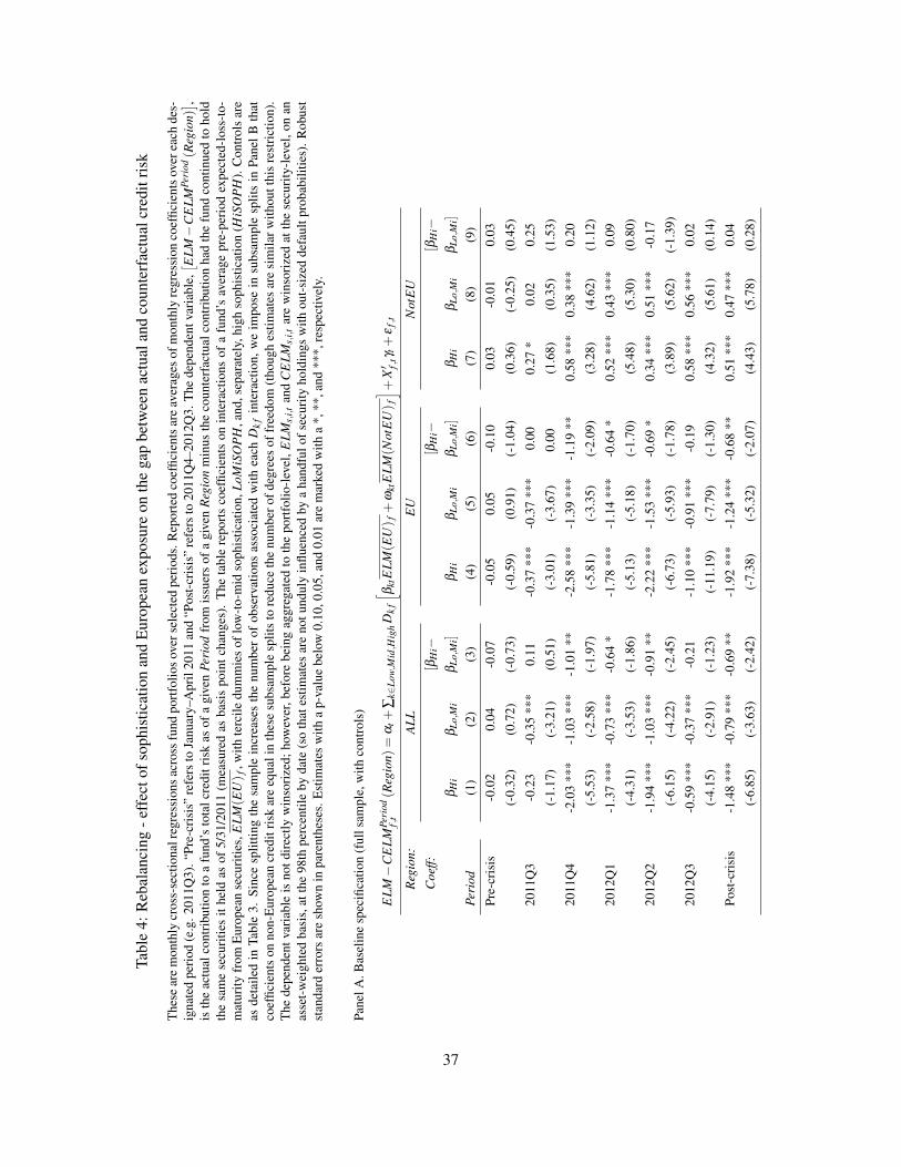
Tabl
e4:
Reb
alan
cing
-eff
ecto
fsop
hist
icat
ion
and
Eur
opea
nex
posu
reon
the
gap
betw
een
actu
alan
dco
unte
rfac
tual
cred
itri
sk
The
sear
em
onth
lycr
oss-
sect
iona
lreg
ress
ions
acro
ssfu
ndpo
rtfo
lios
over
sele
cted
peri
ods.
Rep
orte
dco
effic
ient
sar
eav
erag
esof
mon
thly
regr
essi
onco
effic
ient
sov
erea
chde
s-ig
nate
dpe
riod
(e.g
.201
1Q3)
.“Pr
e-cr
isis
”re
fers
toJa
nuar
y–A
pril
2011
and
“Pos
t-cr
isis
”re
fers
to20
11Q
4–20
12Q
3.T
hede
pend
entv
aria
ble,[ E
LM−
CE
LMPe
riod(R
egio
n)] ,
isth
eac
tual
cont
ribu
tion
toa
fund
’sto
talc
redi
tris
kas
ofa
give
nPe
riod
from
issu
ers
ofa
give
nR
egio
nm
inus
the
coun
terf
actu
alco
ntri
butio
nha
dth
efu
ndco
ntin
ued
toho
ldth
esa
me
secu
ritie
sit
held
asof
5/31
/201
1(m
easu
red
asba
sis
poin
tcha
nges
).T
heta
ble
repo
rts
coef
ficie
nts
onin
tera
ctio
nsof
afu
nd’s
aver
age
pre-
peri
odex
pect
ed-l
oss-
to-
mat
urity
from
Eur
opea
nse
curi
ties,
ELM
(EU)
f,w
ithte
rcile
dum
mie
sof
low
-to-
mid
soph
istic
atio
n,Lo
MiS
OP
H,a
nd,s
epar
atel
y,hi
ghso
phis
ticat
ion
(HiS
OP
H).
Con
trol
sar
eas
deta
iled
inTa
ble
3.Si
nce
split
ting
the
sam
ple
incr
ease
sth
enu
mbe
rof
obse
rvat
ions
asso
ciat
edw
ithea
chD
kf
inte
ract
ion,
we
impo
sein
subs
ampl
esp
lits
inPa
nelB
that
coef
ficie
nts
onno
n-E
urop
ean
cred
itri
skar
eeq
uali
nth
ese
subs
ampl
esp
lits
tore
duce
the
num
bero
fdeg
rees
offr
eedo
m(t
houg
hes
timat
esar
esi
mila
rwith
outt
his
rest
rict
ion)
.T
hede
pend
entv
aria
ble
isno
tdir
ectly
win
sori
zed;
how
ever
,bef
ore
bein
gag
greg
ated
toth
epo
rtfo
lio-l
evel
,ELM
s,i,t
and
CE
LMs,
i,tar
ew
inso
rize
dat
the
secu
rity
-lev
el,o
nan
asse
t-w
eigh
ted
basi
s,at
the
98th
perc
entil
eby
date
(so
that
estim
ates
are
notu
ndul
yin
fluen
ced
bya
hand
fulo
fsec
urity
hold
ings
with
out-
size
dde
faul
tpro
babi
litie
s).R
obus
tst
anda
rder
rors
are
show
nin
pare
nthe
ses.
Est
imat
esw
itha
p-va
lue
belo
w0.
10,0
.05,
and
0.01
are
mar
ked
with
a*,
**,a
nd**
*,re
spec
tivel
y.
Pane
lA.B
asel
ine
spec
ifica
tion
(ful
lsam
ple,
with
cont
rols
)
ELM−
CE
LMPe
riod
f,t
(Reg
ion)
=α
t+∑
k∈Lo
w,M
id,H
igh
Dk
f
[ βkt
ELM
(EU)
f+
ωkt
ELM
(Not
EU)
f] +X′ f,
tγt+
εf,
t
Reg
ion:
ALL
EU
Not
EU
Coe
ff:[β
Hi−
[βH
i−[β
Hi−
βH
iβ
Lo,M
iβ
Lo,M
i]β
Hi
βLo
,Mi
βLo
,Mi]
βH
iβ
Lo,M
iβ
Lo,M
i]
Peri
od(1
)(2
)(3
)(4
)(5
)(6
)(7
)(8
)(9
)
Pre-
cris
is-0
.02
0.04
-0.0
7-0
.05
0.05
-0.1
00.
03-0
.01
0.03
(-0.
32)
(0.7
2)(-
0.73
)(-
0.59
)(0
.91)
(-1.
04)
(0.3
6)(-
0.25
)(0
.45)
2011
Q3
-0.2
3-0
.35
***
0.11
-0.3
7**
*-0
.37
***
0.00
0.27
*0.
020.
25
(-1.
17)
(-3.
21)
(0.5
1)(-
3.01
)(-
3.67
)0.
00(1
.68)
(0.3
5)(1
.53)
2011
Q4
-2.0
3**
*-1
.03
***
-1.0
1**
-2.5
8**
*-1
.39
***
-1.1
9**
0.58
***
0.38
***
0.20
(-5.
53)
(-2.
58)
(-1.
97)
(-5.
81)
(-3.
35)
(-2.
09)
(3.2
8)(4
.62)
(1.1
2)
2012
Q1
-1.3
7**
*-0
.73
***
-0.6
4*
-1.7
8**
*-1
.14
***
-0.6
4*
0.52
***
0.43
***
0.09
(-4.
31)
(-3.
53)
(-1.
86)
(-5.
13)
(-5.
18)
(-1.
70)
(5.4
8)(5
.30)
(0.8
0)
2012
Q2
-1.9
4**
*-1
.03
***
-0.9
1**
-2.2
2**
*-1
.53
***
-0.6
9*
0.34
***
0.51
***
-0.1
7
(-6.
15)
(-4.
22)
(-2.
45)
(-6.
73)
(-5.
93)
(-1.
78)
(3.8
9)(5
.62)
(-1.
39)
2012
Q3
-0.5
9**
*-0
.37
***
-0.2
1-1
.10
***
-0.9
1**
*-0
.19
0.58
***
0.56
***
0.02
(-4.
15)
(-2.
91)
(-1.
23)
(-11
.19)
(-7.
79)
(-1.
30)
(4.3
2)(5
.61)
(0.1
4)
Post
-cri
sis
-1.4
8**
*-0
.79
***
-0.6
9**
-1.9
2**
*-1
.24
***
-0.6
8**
0.51
***
0.47
***
0.04
(-6.
85)
(-3.
63)
(-2.
42)
(-7.
38)
(-5.
32)
(-2.
07)
(4.4
3)(5
.78)
(0.2
8)
37

Pane
lB:S
ubsa
mpl
esp
lits
and
robu
stne
ssch
ecks
ELM−
CE
LMPe
riod
f(R
egio
n)=
αt+
∑3 k=
1
[ βkE
LM(E
U)
f×
Dk
f+
ωkE
LM(N
otE
U)
f×
Dk
f] +X′ fγ
+ε
f
Reg
ion:
ALL
EU
Not
EU
Coe
ff:[β
Hi−
[βH
i−[β
Hi−
βH
iβ
LoM
iβ
LoM
i]β
Hi
βLo
Mi
βLo
Mi]
βH
iβ
LoM
iβ
LoM
i]
Peri
od(1
)(2
)(3
)(4
)(5
)(6
)(7
)(8
)(9
)
B.1
Exc
ludi
ngco
ntro
ls
Post
-cri
sis
-1.3
0**
*-0
.52
***
-0.7
8**
*-1
.65
***
-0.9
1**
*-0
.74
**0.
42**
*0.
40**
*0.
01
(-5.
56)
(-3.
35)
(-2.
79)
(-5.
35)
(-5.
70)
(-2.
12)
(3.0
4)(5
.12)
(0.0
9)
B.2
Subs
ampl
eof
fund
sw
ithbe
low
med
ian
aver
age
bala
nce
size
Post
-cri
sis
-2.7
7**
*-0
.49
*-2
.28
***
-3.7
6**
*-0
.93
***
-2.8
4**
*1.
05**
0.43
***
0.62
(-4.
66)
(-1.
74)
(-3.
63)
(-4.
32)
(-3.
28)
(-3.
19)
(2.4
6)(4
.36)
(1.4
5)
B.3
Subs
ampl
eof
fund
sw
ithab
ove
med
ian
aver
age
bala
nce
size
Post
-cri
sis
-0.8
7**
*-1
.21
***
0.34
-1.2
0**
*-1
.74
***
0.54
0.38
***
0.57
***
-0.1
9
(-3.
05)
(-2.
75)
(0.6
2)(-
3.63
)(-
3.71
)(0
.87)
(3.4
2)(3
.64)
(-0.
97)
B.4
Incl
udin
gin
tera
ctio
nsbe
twee
nso
phis
ticat
ion
bins
and
fund
outfl
ows
duri
ng6/
7–7/
5/20
11
Post
-cri
sis
-1.5
7**
*-0
.82
***
-0.7
4**
-2.0
0**
*-1
.28
***
-0.7
2**
0.51
***
0.47
***
0.04
(-7.
80)
(-3.
85)
(-2.
54)
(-8.
12)
(-5.
61)
(-2.
13)
(4.1
3)(5
.88)
(0.2
6)
B.5
Subs
ampl
eof
fund
sw
ithbe
low
med
ian
outfl
ows
duri
ng6/
7–7/
5/20
11
Post
-cri
sis
-1.4
3**
*-1
.15
***
-0.2
8-1
.89
***
-1.6
5**
*-0
.24
0.66
***
0.50
***
0.16
(-3.
65)
(-2.
80)
(-0.
45)
(-4.
89)
(-3.
86)
(-0.
38)
(5.5
8)(4
.42)
(1.0
0)
B.6
Subs
ampl
eof
fund
sw
ithab
ove
med
ian
outfl
ows
duri
ng6/
7–7/
5/20
11
Post
-cri
sis
-1.3
3**
*-0
.52
-0.8
1-1
.60
***
-0.9
1**
-0.6
90.
26*
0.39
**-0
.13
(-2.
85)
(-1.
05)
(-1.
14)
(-2.
84)
(-1.
98)
(-0.
92)
(1.6
7)(2
.02)
(-0.
52)
38

Table 5: Issuer-level difference-in-difference estimates – effect of issuer region and risk level on MMFinvestment allocations
Using a difference-in-difference regression design of the following form at the issuer-date-level, this table documents that riskierissuers in Europe experienced the largest declines in MMF asset allocations during the eurozone crisis:
Log∆Port f olioWeighti,t = β0(δCrisist ×δ EU
i )+β1(δCrisis
t ×δ EUi ×PDi,t
)+β2
(δCrisis
t ×δ NotEUi ×PDi,t
)+
β3(δ EU
i ×PDi,t)+β4
(δ NotEU
i ×PDi,t)+δ EU
i +δt + εi,t ,
The dependent variable is the logged month-over-month change in issuer i’s total outstanding debt held by prime MMFs (as apercentage of total prime MMF assets), Log∆Port f olioWeighti,t . The crisis indicator, δCrisis, takes the value of 1 after May 2011and 0 before. Issuers headquartered in Europe or outside of Europe are identified with the dummy δ EU
i or δ NotEUi , respectively.
These indicators are interacted with the issuer’s 90-day annualized default probability, PDi,t . All regressions include date fixedeffects, δt . Specified columns restrict securities to CP and CDs (i.e., uncollateralized securities). Columns (3)–(6) also restrict thesample to only those issuers with relatively low credit risk – based on the maximum PDi,t of the issuer over the 2011–2012 period.The dependent variable is winsorized at the 2nd and 98th percentiles across issuers by date.
Regressor (1) (2) (3) (4) (5) (6) (7) (8)
δCrisist ×δ EU
i -0.563*** -0.630*** -0.529*** -0.453** -0.548** -0.476** -0.483*** -0.325*
(-4.383) (-4.000) (-3.426) (-2.563) (-2.610) (-2.066) (-2.879) (-1.746)
δCrisist ×δ EU
i ×PDi,t -0.443** -0.674***
(-2.249) (-3.239)
δCrisist ×δ NotEU
i ×PDi,t -0.093 0.080
(-0.654) (1.124)
δ EUi ×PDi,t 0.053 -0.008
(0.439) (-0.078)
δ NotEUi ×PDi,t 0.083 -0.084
(0.882) (-1.390)
δ EUi 0.035 -0.031 0.082 -0.014 0.048 -0.025 0.043 -0.023
(0.592) (-0.437) (0.988) (-0.135) (0.460) (-0.202) (0.475) (-0.212)
N 2385 1893 1400 1234 1105 979 1821 1581
R2 0.082 0.096 0.073 0.055 0.081 0.053 0.164 0.183
Sample All CP & CDs All CP & CDs All CP & CDs All CP & CDs
Max PD (0,100%) (0,1%) (0,0.5%) (0,100%)
39

Table 6: Security-level difference-in-difference estimates – effect of issuer region and risk level on MMFinvestment maturities
Using a difference-in-difference regression design of the following form at the security-fund-date-level, this table documents thatriskier issuers in Europe experienced the largest declines in maturities on outstanding debt held by MMFs during the eurozonecrisis:
Maturitys,i, f .t = β0(δCrisist ×δ EU
i )+β1(δCrisis
t ×δ EUi ×PDi,t
)+β2
(δCrisis
t ×δ NotEUi ×PDi,t
)+
β3(δ EU
i ×PDi,t)+β4
(δ NotEU
i ×PDi,t)+δi×δ
Categorys +δt ×δ
Categorys + εs, f ,t
The dependent variable is the number of days until final maturity on security of type s issued by issuer i held by fund f ondate t, Maturitys. f .t . The post period indicator, δCrisis
t , takes the value 1 after May 2011 and 0 before. Issuers headquartered inEurope or outside of Europe are identified with the dummy δ EU
i and δ NotEUi , respectively. These indicators are interacted with
the issuer’s 90-day annualized default probability, PDi,t . All regressions include issuer × security category and date × securitycategory fixed effects, δi× δ
Categorys and δt × δ
Categorys , respectively. Even-numbered columns restrict securities to CP and CDs
(i.e., uncollateralized securities). Columns (3)–(6) also restrict the sample to only those issuers with relatively low credit risk –based on the maximum PDi,t of the issuer over the 2011–2012 period. The dependent variable is winsorized at the 98th percentileacross securities by date.
(1) (2) (3) (4) (5) (6) (7) (8)
δCrisist ×δ EU
i -33.310*** -42.680*** -23.086*** -25.922*** -24.740*** -21.289** -25.263*** -27.033***
(-7.563) (-5.599) (-4.283) (-3.417) (-3.960) (-2.335) (-4.091) (-2.994)
δCrisist ×δ EU
i ×PDi,t -10.590* -26.931***
(-1.732) (-3.244)
δCrisist ×δ NotEU
i ×PDi,t -0.018 -1.583
(-0.007) (-0.487)
δ EUi ×PDi,t 3.972 12.682
(0.641) (1.530)
δ NotEUi ×PDi,t 2.204 6.845
(0.279) (0.882)
N 111765 60501 66359 37514 45437 25716 102283 56245
R2 0.534 0.374 0.546 0.358 0.541 0.354 0.527 0.365
Sample All CP & CDs All CP & CDs All CP & CDs All CP & CDs
Max PD (0,100%) (0,1%) (0,0.5%) (0,100%)
40

8/2/2011
6/7/2011, 1.1
7/5/2011, -9.0
-30
-20
-10
0
10
20
30
17-May-11 17-Jun-11 17-Jul-11 17-Aug-11 17-Sep-11 17-Oct-11 17-Nov-11
Per
cen
tage
Ch
ange
in A
sset
s
Government
Prime
Eurozone
(rapid)Eurozone
(slow)
Debt
Ceiling
Figure 1: Aggregate MMF institutional shareclass flows
This figure shows the change in aggregate institutional shareclass assets of MMFs from May 17–December 16 of 2011. Changesin assets are normalized by asset values on May 17, 2011. The graph shows flows split by investment objective (i.e., prime versusgovernment-only MMFs).
100
150
200
250
300
350
400
Jan-1
1
Feb
-11
Mar
-11
Apr-
11
May
-11
Jun-1
1
Jul-
11
Aug-1
1
Sep
-11
Oct
-11
Nov-1
1
Dec
-11
Jan-1
2
Feb
-12
Mar
-12
Apr-
12
May
-12
Jun-1
2
Jul-
12
Aug-1
2
Sep
-12
Oct
-12
Nov-1
2
Dec
-12
5-y
ear
CD
S p
rem
ium
(bps)
European
U.S.
Asia/Pacific
Figure 2: 5-Year CDS premiums for banks by region, 2011
The CDS premium for European financials is the iTraxx senior financial index for Europe. The CDS premiums for large Asia/Pacificand U.S. banks is the average of 5-year CDS premiums for (Sumitomo Bank and Mizuho Bank, National Australia Bank, Westpac,and ANZ) and (Bank of America, JPMorgan Chase, Citi, Wells Fargo, and Goldman Sachs), respectively. Canadian banks areexcluded because their CDS is thinly traded.
41

����
���
���
���
$YJ����RI�QHZ
V�VWRULHV��LQGH[HG�WR������
����P�
����P�
����P�
����P�
'DWH
$PHULFDV$VLD�3DFLILF(XURSH
Figure 3: Volume of Media Coverage for MMF Issuers, by Region, 2010-2012
The figure presents indices of daily media attention by region. The y-axis variable is the average number of news reports onBloomberg referencing MMF issuers each day, by region of issuer headquarters, indexed to 100 as of January 1, 2010.
0
50
100
150
200
250
300
350
0
5
10
15
20
25
30
35
40
45
50
Jan
-11
Feb
-11
Mar
-11
Ap
r-1
1
May
-11
Jun-1
1
Jul-
11
Au
g-1
1
Sep
-11
Oct
-11
No
v-1
1
Dec
-11
Jan
-12
Feb
-12
Mar
-12
Ap
r-1
2
May
-12
Jun-1
2
Jul-
12
Au
g-1
2
Sep
-12
Oct
-12
No
v-1
2
Dec
-12
CD
S (
bp
s)
Fu
nd
cre
dit
ris
k (
bp
s)
ELM Counterfactual ELM (CELM) Yield spread European CDS
Figure 4: Credit risk measures over time
This figure shows the asset-weighted average credit risk in prime MMFs (LHS) and the CDS premium for the iTraxx senior financialindex for Europe (RHS). The credit risk in prime MMFs as of month-end is measured in 3 ways: the annualized expected-loss-to-maturity (ELM), the counterfactual annualized ELM had prime funds continued to hold their end-May portfolio allocations(CELM), and the annualized gross yield on each prime MMF minus the yield on the average government MMF (Yield spread).
42
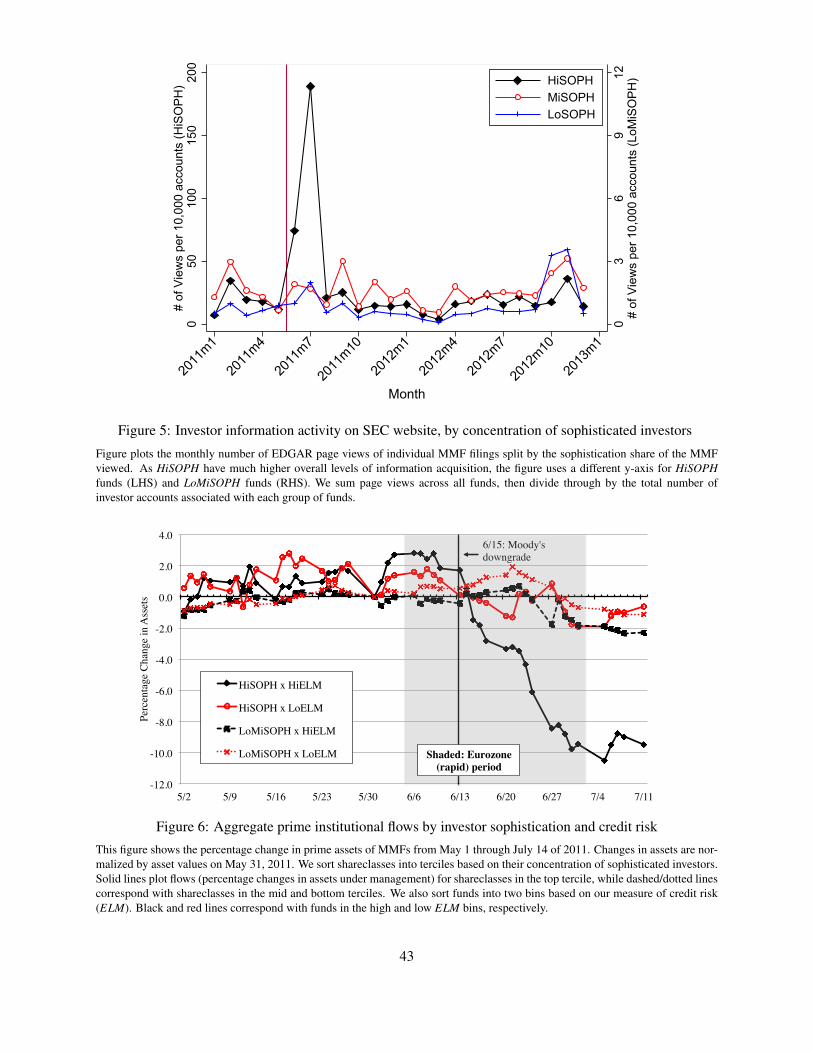
03
69
12#
of V
iew
s pe
r 10,
000
acco
unts
(LoM
iSO
PH)
050
100
150
200
# of
Vie
ws
per 1
0,00
0 ac
coun
ts (H
iSO
PH)
2011
m1
2011
m4
2011
m7
2011
m10
2012
m1
2012
m4
2012
m7
2012
m10
2013
m1
Month
HiSOPHMiSOPHLoSOPH
Figure 5: Investor information activity on SEC website, by concentration of sophisticated investors
Figure plots the monthly number of EDGAR page views of individual MMF filings split by the sophistication share of the MMFviewed. As HiSOPH have much higher overall levels of information acquisition, the figure uses a different y-axis for HiSOPHfunds (LHS) and LoMiSOPH funds (RHS). We sum page views across all funds, then divide through by the total number ofinvestor accounts associated with each group of funds.
-12.0
-10.0
-8.0
-6.0
-4.0
-2.0
0.0
2.0
4.0
5/2 5/9 5/16 5/23 5/30 6/6 6/13 6/20 6/27 7/4 7/11
Perc
enta
ge C
hang
e in
Ass
ets
HiSOPH x HiELM
HiSOPH x LoELM
LoMiSOPH x HiELM
LoMiSOPH x LoELM
6/15: Moody's downgrade
Shaded: Eurozone (rapid) period
Figure 6: Aggregate prime institutional flows by investor sophistication and credit risk
This figure shows the percentage change in prime assets of MMFs from May 1 through July 14 of 2011. Changes in assets are nor-malized by asset values on May 31, 2011. We sort shareclasses into terciles based on their concentration of sophisticated investors.Solid lines plot flows (percentage changes in assets under management) for shareclasses in the top tercile, while dashed/dotted linescorrespond with shareclasses in the mid and bottom terciles. We also sort funds into two bins based on our measure of credit risk(ELM). Black and red lines correspond with funds in the high and low ELM bins, respectively.
43

Figure 7: Rebalancing - actual vs. counterfactual credit risk by region
This figure plots the coefficient estimates of βk in Equation 2 based on a series of monthly cross-sectional regressions. Depen-dent variables are either
[ELM−CELMPeriod
f (Region)]
for regions specified above the plots. Explanatory variables capture theinteraction effect between a fund’s pre-period average European credit risk exposure and its investor sophistication tercile.
P25
P50
P75
P90
050
100
150
200
2011
q1
2011
q2
2011
q3
2011
q4
2012
q1
2012
q2
2012
q3
2012
q4
Europe Not Europe
Panel A: All new securities
P25
P50
P75
P90
050
100
150
200
2011
q1
2011
q2
2011
q3
2011
q4
2012
q1
2012
q2
2012
q3
2012
q4
Europe Not Europe
Panel B: New CP and CD securities
Figure 8: Security maturities by issuer default probability, region, and date
The figure plots the number of days until maturity (y-axis) by date (x-axis). Solid and dashed lines identify securities from Europeand from outside of Europe, receptively. The figure plots the 25th, 50th, 75th, and 90th percentiles of the cross-sectional distributionof maturities (in calendar days) of new securities which are added to funds’ portfolios in each calendar quarter. Panel A uses the fullsample of securities. Panel B restricts the sample to CP and CD security categories, which are generally uncollateralized categories.
44

A Additional Results Not Included in Main Text
Data construction
Appendix Figure A1 depicts information about each of these data sources and the process used to compile
them. Our first data source consists of a complete record of the portfolio holdings of all prime MMFs at
each month-end in the 2011–2012 period. The SEC’s 2010 Amendments require each MMF, starting in
November 2010, to file Form N-MFP each month with the SEC. We obtain this detailed monthly portfolio-
level holdings information from SEC’s Edgar data site. With respect to each portfolio security, the fund
must report the name of the issuer, details about the issue (e.g., the type of security and whether it is
collateralized), and the security’s maturity. We categorize the holdings on Form N-MFP by the parent of the
issuer. Second, we hand match firms in the RMI database with the list of parent companies that issue debt to
MMFs from our N-MFP data. Third, we use a unique database from the Investment Company Institute (ICI)
consisting of the proportion of assets, for each MMF shareclass, held by broad categories of investors at
the start of 2011. This data also contains detail on the number of accounts associated with each shareclass.
Finally, we use a separate data source, iMoneyNet.com, to calculate investor flows to/from both individual
shareclasses and individual funds during the Eurozone crisis, along with several other explanatory variables.
We join the RMI/N-MFP data set with ICI and iMoneyNet data based on EDGAR identifiers, CIK codes,
and tickers.
45
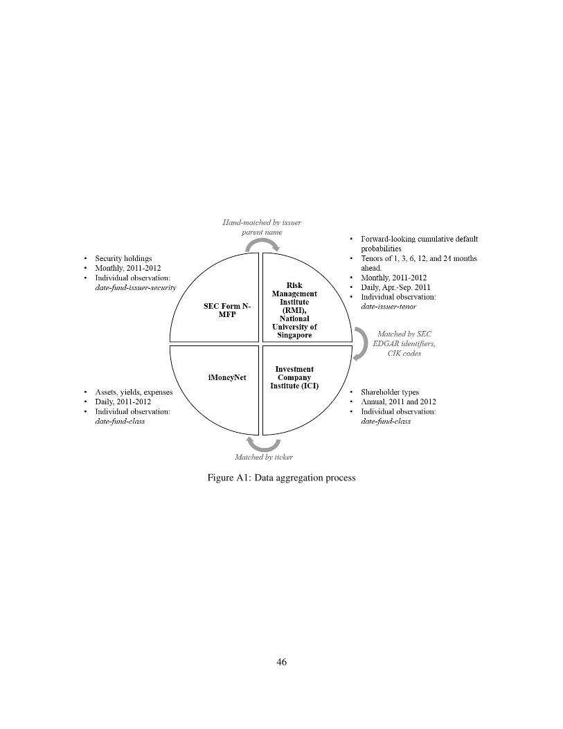
Figure A1: Data aggregation process
46

Shareclass-level descriptive statistics
Appendix Table A1 presents statistics for key variables used in our fund flow regressions at the shareclass
level (i.e., regressions shown in Table 2). The right-most columns compare shareclasses with low and mid
sophisticated ownership to those with high sophisticated ownership. Of note is the wide variation in flows
(standard deviation of 8% of assets) experienced by shareclasses during the period of heavy redemptions
(6/7-7/5/2011). Sophisticated ownership is also widely distributed (standard deviation of 32% of assets).
The last columns indicate that HiSOPH shareclasses experienced significantly more outflows relative to
LoMiSOPH shareclasses, consistent with greater monitoring behavior. HiSOPH shareclasses also tend to
have about 3 basis points more credit risk (ELM), on average during the period of heavy redemptions,
than do LoMiSOPH shareclasses. The differential risk is primarily attributable to European securities. We
control for this difference in regressions (Table 2) by separately controlling for sophistication and evaluating
the interaction effect between sophistication and credit risk. HiSOPH shareclasses also tend to be larger
(ASSETS) and higher yielding funds (GYIELD). As expected, they are more likely to be designated as
“institutional” in their prospectus (INST).
47

Table A1: Shareclass-level descriptive Statistics, summer redemption period (6/7–7/5/2011)
These are descriptive statistics for key dependent and explanatory variables only. Class-level and fund-level (a.k.a., portfolio-level)variables are denoted by the subscript “c” and “ f ”, respectively. Flow variables are measured as a percentage of class or fund assetsduring the period of rapid redemptions, 6/7/2011–7/5/2011. Credit risk is measured as the expected-loss-to-maturity (ELM f ) onthe fund’s portfolio (measured in basis points). Unless otherwise dated, this variable is averaged across days during 6/7–7/5/2011.The “counterfactual” credit risk, measured as the expected-loss-to-maturity on 9/30/2011 had the fund continued to hold the sameportfolio securities it held as of 5/31/2011 (CELM f ). SOPH is the portion of class or fund assets held by sophisticated investors.
ALL LoMiSOPH HiSOPH LoMi - Hi
mean sd p10 p50 p90 mean mean t-stat
FLOWc(%) -2.24 8.07 -14.30 -0.85 7.23 -0.85 -5.04 (5.08)
SOPHc1/1/11 (%) 23.15 32.63 0.00 4.12 85.84 3.46 62.77 (-26.77)
ELM f (bps) 14.49 6.37 5.66 14.39 23.92 13.49 16.42 (-4.97)
ELM f (EU) (bps) 10.38 5.57 1.7 10.86 16.16 9.32 12.55 (-6.10)
ELM f (NotEU) (bps) 4.11 2.83 1.38 3.44 8.14 4.17 3.87 (1.17)
CELM f 9/30/2011 (bps) 30.24 12.48 12.09 31.96 44.39 28.11 34.36 (-5.42)
CELM f (EU) 9/30/2011 (bps) 23.47 12.13 4.28 24.96 36.02 21.14 28.20 (-6.20)
CELM f (NotEU) 9/30/11 (bps) 6.77 3.58 3.26 6.15 11.87 6.97 6.16 (2.46)
ASSET Sc6/7/2011 ($ mil) 3175.57 9956.38 16.70 402.30 6876.20 2149.64 5239.93 (-3.01)
ASSET S f 6/7/2011 ($ mil) 13522.11 26456.09 280.30 2586.40 32047.90 9627.11 21359.61 (-4.21)
BALSIZE f 5/31/11 ($ mil) 0.02 0.08 0.00 0.00 0.04 0.02 0.03 (-1.46)
GY IELDc(bps) 24.33 5.69 16.70 25.03 30.48 23.75 25.50 (-3.57)
INSTc 5/31/2011 [0,1] 0.51 0.50 0.00 1.00 1.00 0.30 0.92 (-18.71)
N 494 330 164
Alternative flow regression specification using EDGAR traffic as a proxy for investor infor-
mation processing capacity
In the main text, we use survey data on shareholder composition as our proxy for investor information
acquisition costs. Here, we present the results from a specification which instead uses the number of hits
on the SEC EDGAR webiste from January through June 2011, relative to the number of accounts, as an
alternative measure of investor monitoring intensity. Note that a nontrivial fraction of these page views were
associated with a SEC press release that announced the introduction of Form-NMP.
Similar to the regressions in Table 2, we sort funds into categories based on the level of activity on
the EDGAR site then run a sequence of regressions to predict flows in Table A2. There are two minor
differences relative to the specification described in the text. First, since we cannot allocate traffic across
shareclasses, we run the analysis at the fund level. Second, as this measure is somewhat noisier than our
baseline sophistication measure, we sort funds into two (rather than three) categories. We also omit pre-crisis
48

coefficients for brevity. Otherwise, the empirical specification and layout is identical to columns (4-10) of
Table 2. As is clear from the table, estimates have similar signs and statistical significance to those obtained
in the main text. If anything, magnitudes are slightly higher relative to estimates in Table 2.
Table A2: Flow regressions: the influence of credit risk and investor sophistication (as defined by EDGARpage views)
The dependent variable (FLOW f ,t ) is the percentage change in the assets of class, f , during month, t. Key explanatory variablesare interactions of fund credit risk and its investor sophistication – high/low dummies generated from the distribution of number ofEDGAR page views relative to the number of accounts as of the start of the year. The credit risk measures used in these interactionsdiffer according to their moment of measurement and the regional origin of the securities included in the measure. These differencesare marked at the top of the table (“EU” is an abreviation of Europe). Columns (1)–(7) use cross-sectional regressions over theperiod of heavy redemptions (6/7–7/5/2011). All regressions include a high views bin (HiV IEWS f ) dummy. Additional controlsare investor sophistication in continuous form (SOPH f ), the fraction of assets under management designated as “institutional” inthe fund’s prospectus (INSTf ), the logged total net assets of the class and the fund (ASSET S f ,t−1 and ASSET S f ,t−1, respectively),the fund’s annualized gross yield (GY IELD f ,t−1), the asset weighted average of shareclass-level logged historical asset variation(FLOWST Dc,t−1), the log of the average balance size for the fund (BALSIZE f ), and the share of fund assets not maturing duringthe month nor invested in Treasury/Agency securities (ILLIQUIDITY f ). Pre-crisis panel regressions include time fixed effects.To manage tax season-related outliers, the FLOW f ,t and FLOWST D f ,t−1 are both winsorized at the 2nd and 98th percentiles. Inparentheses are t-statistics, calculated using standard errors clustered at the fund portfolio level. The penultimate row provides thep-value from a two-sided test that the coefficient on ELM (All or EU) x LoVIEWS equals the coefficient on ELM (All or EU) xHiVIEWS. Estimates with a p-value below 0.10, 0.05, and 0.01 are marked with a *, **, and ***, respectively.
Crisis period: June 7 - July 5, 2011
ELM measure: Prior month-end ELM September 2011 Counterfactual ELM
Aggregation level for ELM: All All EU EU All EU EU
(1) (2) (3) (4) (5) (6) (7)
ELM (All or EU) x LoVIEWS -0.106 0.026 -0.030 -0.044 0.007 -0.005 -0.010
(-1.589) (0.330) (-0.297) (-0.415) (0.172) (-0.112) (-0.211)
ELM (All or EU) x HiVIEWS -0.488*** -0.212* -0.496*** -0.528*** -0.146** -0.205*** -0.209***
(-4.594) (-1.738) (-3.565) (-3.712) (-2.348) (-3.200) (-3.268)
ELM (NotEU) x LoVIEWS 0.171 0.091
(0.860) (0.648)
ELM (NotEU) x HiVIEWS 0.458** 0.282
(2.001) (1.453)
N 183 183 183 183 183 183 183
R2 0.10 0.32 0.35 0.37 0.33 0.34 0.35
P value (HML) 0.003 0.063 0.002 0.002 0.020 0.004 0.005
Controls No Yes Yes Yes Yes Yes Yes
49
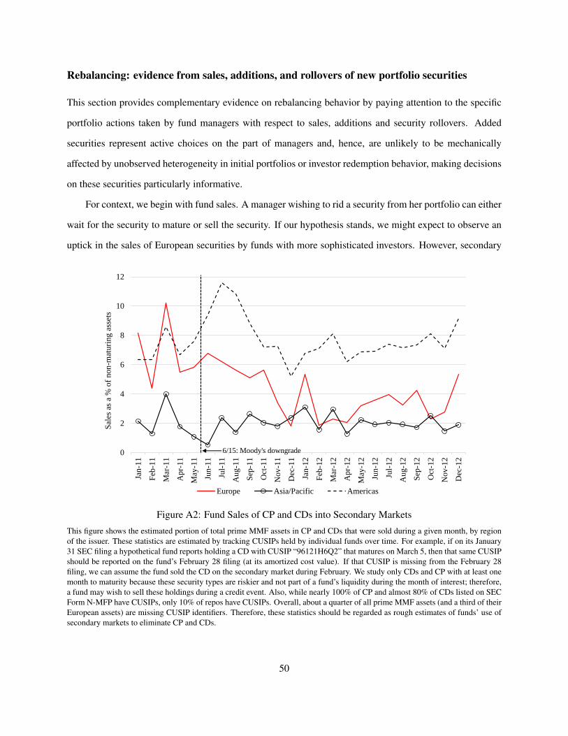
Rebalancing: evidence from sales, additions, and rollovers of new portfolio securities
This section provides complementary evidence on rebalancing behavior by paying attention to the specific
portfolio actions taken by fund managers with respect to sales, additions and security rollovers. Added
securities represent active choices on the part of managers and, hence, are unlikely to be mechanically
affected by unobserved heterogeneity in initial portfolios or investor redemption behavior, making decisions
on these securities particularly informative.
For context, we begin with fund sales. A manager wishing to rid a security from her portfolio can either
wait for the security to mature or sell the security. If our hypothesis stands, we might expect to observe an
uptick in the sales of European securities by funds with more sophisticated investors. However, secondary
0
2
4
6
8
10
12
Jan-1
1
Feb
-11
Mar
-11
Ap
r-1
1
May
-11
Jun
-11
Jul-
11
Au
g-1
1
Sep
-11
Oct
-11
No
v-1
1
Dec
-11
Jan
-12
Feb
-12
Mar
-12
Ap
r-1
2
May
-12
Jun-1
2
Jul-
12
Au
g-1
2
Sep
-12
Oct
-12
No
v-1
2
Dec
-12
Sal
es a
s a
% o
f n
on
-mat
uri
ng a
sset
s
Europe Asia/Pacific Americas
6/15: Moody's downgrade
Figure A2: Fund Sales of CP and CDs into Secondary Markets
This figure shows the estimated portion of total prime MMF assets in CP and CDs that were sold during a given month, by regionof the issuer. These statistics are estimated by tracking CUSIPs held by individual funds over time. For example, if on its January31 SEC filing a hypothetical fund reports holding a CD with CUSIP “96121H6Q2” that matures on March 5, then that same CUSIPshould be reported on the fund’s February 28 filing (at its amortized cost value). If that CUSIP is missing from the February 28filing, we can assume the fund sold the CD on the secondary market during February. We study only CDs and CP with at least onemonth to maturity because these security types are riskier and not part of a fund’s liquidity during the month of interest; therefore,a fund may wish to sell these holdings during a credit event. Also, while nearly 100% of CP and almost 80% of CDs listed on SECForm N-MFP have CUSIPs, only 10% of repos have CUSIPs. Overall, about a quarter of all prime MMF assets (and a third of theirEuropean assets) are missing CUSIP identifiers. Therefore, these statistics should be regarded as rough estimates of funds’ use ofsecondary markets to eliminate CP and CDs.
50

markets for short-term securities, like CDs and CP, are famously thin (Covitz and Downing, 2007) and
are even thinner for non-U.S. issued debt. Accordingly, we estimate that monthly fund sales account for
under 5% of assets, on average, over 2011–2012. We arrive at this figure by tracking CUSIPs on fund
holdings over time. Non-maturing CUSIPs that do not appear in a fund’s portfolio as of the next month-end
are assumed to have been sold onto secondary markets.45 The results are presented in Figure A2. Fund
sales of U.S. paper rose during the summer of 2011, while, at the same time, fund sales of European paper
slumped and remained low throughout the Eurozone crisis. Falling liquidity and, hence, lower secondary
market prices for European paper might explain why just 3% of funds’ European CP and CDs were sold
into secondary markets during the peak of the Eurozone crisis in November of 2011. This is consistent with
our earlier observation that the rebalancing accelerated after October 2011 (see Figure 7), well after the
summer’s redemptions.
The graph suggests that funds with sophisticated investors likely held European paper until maturity,
then refrained from replacing it with new European issues, or replaced it with shorter maturing and/or better
collateralized issues. We, therefore, do not attempt to model heterogeneity in security sales across funds
and, instead, turn our attention to securities that are added to fund portfolios during the crisis. Prior analyses
suggest an excess supply of dollar-denominated short-term debt from European banks during the Eurozone
crisis (Correa et al., 2013; Ivashina et al., 2015) and, hence, a variety of securities for MMF managers to
choose from – enabling an analysis of heterogeneity in selections across funds.46
Using the same regression specification from Equation (2), Table A3 presents cross-sectional estimates
relating new security risks (dependent variable) with funds’ initial European exposures and sophistication
during the crisis. The first dependent variable in the table captures the European share of risk (ELM) coming
from CUSIPs that appear in a fund’s portfolio for the first time in a given month (EU%o f NewELM).47
The baseline correlation in the pre-crisis period (February-May 2011, since we lose one month of data to
identify new securities) is positive and significant for both HiSOPH and LoMiSOPH funds, which simply
implies that MMFs with higher (lower) initial European ELM tend to have larger fractions of new portfolio
45Note that securities with CUSIPS are mostly CP and CD securities; repo tend not to have CUSIPs.46Note also the roughly $85 billion uptick in the dollar-denominated borrowing of European banks from the European Central
Bank (ECB) “swap line” in December of 2011. The ECB swap line has been cited as one of the ways that European banks replacedfinancing from MMFs over the period. See: https://www.ici.org/pdf/per19-01.pdf
47To be consistent with our earlier analysis, we winsorize dependent variables at the 95th percentile, though results are similarif we do not winsorize.
51

risk coming from (outside) Europe. Importantly, the slope coefficients between HiSOPH and LoMiSOPH
funds are indistinguishable. Starting in 2011Q3 and continuing through the post-crisis (2011Q4-2012Q3),
LoMiSOPH funds with initially higher European exposures maintain their higher share of new securities
risk coming from Europe. In sharp contrast, the coefficient changes sign for HiSOPH funds, a substantial
decrease to -0.23 from the pre-crisis baseline estimate of 0.59, and this negative estimate persists throughout
the crisis (although it is marginally significant only during the post-crisis period). The difference between
β3t and the average of β1t and β2t is highly statistically significant in the post-crisis, consistent with a much
sharper reallocation away from Europe among funds serving the most sophisticated investors.
Next, we compute a measure of weighted-average issuer credit risk (PDNew), which is the 90-day
annualized default probability of issuers of new portfolio CUSIPs, weighted by the share of fund assets.
We do this separately for European and non-European securities. Pre-crisis estimates suggest that, to some
extent, funds with higher initial European exposures achieved them by allocating more funding towards
riskier European issuers. Consistent with what we would expect to observe from the European component
of a passive portfolio, these coefficients become larger for LoMiSOPH funds in the post-crisis period. In
contrast, the estimates become smaller and remain insignificant for HiSOPH funds. Differences between the
two groups are statistically significant from 2011Q3 onward with respect to new European holdings only.
Finally, we compute a measure of the probability of rolling over maturing securities (ProbRoll). Specif-
ically, for each security due to mature in a given calendar month, we construct a dummy variable which
equals one if we see a new issuer-maturity date-security category combination that had not yet appeared in
a prior portfolio and zero otherwise. The dependent variable a weighted average of these dummy variables,
using the market value of maturing securities as weights, for each month. For European rollover opportuni-
ties, the βk,t’s are modestly negative and insignificantly different from zero in the pre-period, but they diverge
sharply in the post-period. Beginning in 2011Q3 and continuing throughout the post-period, HiSOPH funds
with higher initial European exposures are less likely to roll over maturing positions, whereas LoMiSOPH
funds with higher initial European exposures are more likely to roll over maturing positions. Differences
between the groups are also highly significant.
A consistent pattern in Table A3 is the significant differences, as soon as 2011Q3, in the βk,t estimates.
Recall, that when [ELM−CELM] is the dependent variable (Table 4) significant differences in the βk,t’s do
52

not arise until Q42011. This suggests that it takes more time to alter rebalancing measures computed from
the entire portfolio than to adjust measures based only on new holdings or on rollovers.
Table A3: Rebalancing - effect of sophistication and European exposure on new security choice
These are monthly cross-sectional regressions across fund portfolios over selected periods. Reported coefficients are averages ofmonthly regression coefficients over each designated period (e.g. 2011Q3). “Pre-crisis” refers to January–April 2011 and “Post-crisis” refers to 2011Q4–2012Q3. The first dependent variable measures the European share of ELM from new portfolio securities(EU%o f NewELM,). The second dependent variable captures the asset-weighted average 90-day annualized default probabil-ity on the issuers of a fund’s new portfolio securities (PDNew). Securities are determined to be “new” if the associated CUSIPwas not in the fund’s portfolio as of the prior month-end. The third dependent variable captures the probability that a maturingsecurity is rolled-over (ProbRoll) – measured as whether a maturing fund-issuer-maturity date-security category combination reap-pears the next month (weighted by the dollar value). The table reports coefficients on interactions of a fund’s average pre-periodexpected-loss-to-maturity from European securities, ELM(EU) f , with tercile dummies of low-to-mid sophistication, LoMiSOPH,and, separately, high sophistication (HiSOPH). Controls are as detailed in Table 3. Before being aggregated to the portfolio-level,both ELM and PD are winsorized at the security-level, on an asset-weighted basis, at the 98th percentile by date (so that estimatesare not unduly influenced by a handful of security holdings with out-sized default probabilities). Robust standard errors are shownin parentheses. Estimates with a p-value below 0.10, 0.05, and 0.01 are marked with a *, **, and ***, respectively.
REBALANCINGPeriodf (Region) = αt +∑
3k=1
[βkELM(EU) f ×Dk f +ωkELM(NotEU) f ×Dk f
]+X ′f γ + ε f
Region: EU NotEU
Coeff: [β3=Hi− [β3=Hi−β3=Hi β1,2=Lo,Mi β1,2=Lo,Mi] β3=Hi β1,2=Lo,Mi β1,2=Lo,Mi]
Dependent variable (Y f ) Period (1) (2) (3) (4) (5) (6)
EU%o f NewELM
Pre-crisis 0.59 1.17 *** -0.58 - - -
(1.37) (3.20) (-1.02) - - -
2011Q3 -0.23 1.67 *** -1.90 *** - - -
(-0.41) (3.72) (-2.84) - - -
Post-crisis -0.65 * 2.04 *** -2.69 *** - - -
(-1.77) (4.55) (-4.87) - - -
PDNew
Pre-crisis 0.22 0.44 *** -0.22 0.05 0.03 0.02
(1.61) (4.28) (-1.38) (0.92) (1.10) (0.29)
2011Q3 0.19 0.71 *** -0.53 * 0.16 0.16 ** 0.00
(0.77) (4.26) (-1.84) (1.28) (2.40) (0.03)
Post-crisis -0.18 0.49 *** -0.67 *** 0.16 0.22 *** -0.06
(-0.90) (3.46) (-2.82) (1.61) (3.15) (-0.49)
ProbRoll
Pre-crisis -0.35 -0.21 -0.13 -1.20 ** -0.98 ** -0.22
(-1.03) (-0.62) (-0.28) (-2.47) (-2.09) (-0.34)
2011Q3 -0.82 ** 0.59 -1.42 ** -0.18 -0.38 0.20
(-2.34) (1.18) (-2.44) (-0.47) (-0.71) (0.32)
Post-crisis -0.52 ** 1.32 *** -1.84 *** -0.24 0.50 * -0.74 **
(-2.17) (3.95) (-4.38) (-1.01) (1.91) (-2.07)
53
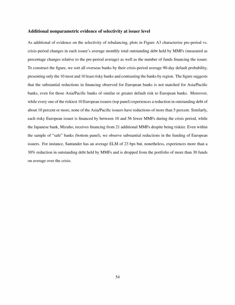
Additional nonparametric evidence of selectivity at issuer level
As additional of evidence on the selectivity of rebalancing, plots in Figure A3 characterize pre-period vs.
crisis-period changes in each issuer’s average monthly total outstanding debt held by MMFs (measured as
percentage changes relative to the pre-period average) as well as the number of funds financing the issuer.
To construct the figure, we sort all overseas banks by their crisis-period average 90-day default probability,
presenting only the 10 most and 10 least risky banks and contrasting the banks by region. The figure suggests
that the substantial reductions in financing observed for European banks is not matched for Asia/Pacific
banks, even for those Asia/Pacific banks of similar or greater default risk to European banks. Moreover,
while every one of the riskiest 10 European issuers (top panel) experiences a reduction in outstanding debt of
about 10 percent or more, none of the Asia/Pacific issuers have reductions of more than 5 percent. Similarly,
each risky European issuer is financed by between 10 and 56 fewer MMFs during the crisis period, while
the Japanese bank, Mizuho, receives financing from 21 additional MMFs despite being riskier. Even within
the sample of “safe” banks (bottom panel), we observe substantial reductions in the funding of European
issuers. For instance, Santander has an average ELM of 23 bps but, nonetheless, experiences more than a
30% reduction in outstanding debt held by MMFs and is dropped from the portfolio of more than 30 funds
on average over the crisis.
54

-60 -40 -20 0 20%∆ Outstanding
KBC(134bp)DanskeBank(138bp)
AxisBank(174bp)RBS(175bp)
Barclays(177bp)Macquarie(181bp)
SocGenerale(186bp)ICICIBank(188bp)
DEXIA(204bp)MizuhoBank(304bp)
-60 -40 -20 0 20∆ # of funds financing
Europe Asia/Pacific
-60 -40 -20 0 20%∆ Outstanding
ComwealthAus(3bp)Aus&NZBank(9bp)
NRWBank(9bp)TokyoMitsu.(10bp)
UnitedOvers.(13bp)StandardCh.(15bp)
HSBC(19bp)SvenskaHand.(19bp)
BilbaoVicaya(20bp)Santander(23bp)
-60 -40 -20 0 20∆ # of funds financing
Mos
t ris
ky 1
0 ba
nks
Leas
t ris
ky 1
0 ba
nks
Figure A3: Rebalancing - differential treatment of issuers by region
This figure plots how the funding relationships between U.S. MMFs and overseas banks changed before and after the start ofheavy redemptions from MMFs due to the Eurozone crisis. Plots show changes in outstanding and number of funds, averagedover January through May 2011 (“pre-crisis”) and, separately, over June 2011 through September 2012 (the full Eurozone “crisis”period). In parentheses is the annualized 90-day default probability on the issuer, averaged over each month-end in the post periodduring which the issuer had outstanding to at least one fund. In other words, if no fund holds the issuer in a given month, thatissuer’s default probability for that month is excluded in its post-period average. We restrict the sample of issuers to those with atleast $10 million outstanding on average during either period.
Additional rebalancing analysis
Appendix Table A4 presents estimates of the coefficients on the interactions between fund sophistication
categories and pre-period, non-European credit risk (ωk,t in Equation 2). The layout is identical to Tables
3 and 4, where different columns are associated with overall, European, and non-European counterfactual
ELM/rebalancing, though we omit some subperiods for brevity. Panel A corresponds with the specification
in Table 3. In panel A, the dependent variable is the fund’s counterfactual credit risk (CELM), holding the
fund’s portfolio fixed at its May 31st 2011 level. We observe that initial non-European exposures predict
55

Tabl
eA
4:R
ebal
anci
ng-t
heef
fect
ofso
phis
ticat
ion
and
non-
Eur
opea
nex
posu
reon
actu
alan
dco
unte
rfac
tual
cred
itri
sk
The
sear
em
onth
lycr
oss-
sect
iona
lre
gres
sion
sac
ross
fund
port
folio
sov
erse
lect
edpe
riod
s.R
epor
ted
coef
ficie
nts
are
aver
ages
ofm
onth
lyre
gres
sion
coef
ficie
nts
over
the
desi
gnat
edpe
riod
(e.g
.20
11Q
3).
“Pre
-cri
sis”
refe
rsto
Janu
ary–
Apr
il20
11an
d“P
ost-
cris
is”
refe
rsto
2011
Q4–
2012
Q3.
The
depe
nden
tvar
iabl
esar
etw
om
easu
res
offu
ndpo
rtfo
liore
bala
ncin
g:C
ELM
Peri
odf
(Reg
ion)
(Pan
elA
)an
dE
LM−
CE
LMPe
riod
f(R
egio
n)(P
anel
B),
asde
scri
bed
inin
Tabl
es3
and
4,re
spec
tivel
y.U
nlik
eth
ose
tabl
es,t
his
tabl
ere
port
sco
effic
ient
son
inte
ract
ions
ofa
fund
’sav
erag
epr
e-pe
riod
expe
cted
-los
s-to
-mat
urity
from
non-
Eur
opea
nse
curi
ties,
ELM
(Not
EU)
f,w
ithte
rcile
dum
mie
sof
soph
istic
atio
n.R
obus
tsta
ndar
der
rors
are
show
nin
pare
nthe
ses.
Est
imat
esw
itha
p-va
lue
belo
w0.
10,0
.05,
and
0.01
are
mar
ked
with
a*,
**,a
nd**
*,re
spec
tivel
y.R
EBA
LAN
CIN
GPe
riod
f(R
egio
n)=
α+
∑3 k=
1
[ βkE
LM(E
U)
f×
Dk
f+
ωkE
LM(N
otE
U)
f×
Dk
f] +X′ fγ
+ε
f
Reg
ion:
ALL
EU
Not
EU
[ω3=
Hi−
[ω3=
Hi−
[ω3=
Hi−
ω3=
Hi
ω1,
2=Lo
,Mi
ω1,
2=Lo
,Mi]
ω3=
Hi
ω1,
2=Lo
,Mi
ω1,
2=Lo
,Mi]
ω3=
Hi
ω1,
2=Lo
,Mi
ω1,
2=Lo
,Mi]
Peri
od(1
)(2
)(3
)(4
)(5
)(6
)(7
)(8
)(9
)
Pane
lA.D
epen
dent
vari
able
:CE
LMPe
riod
f(R
egio
n)
Pre-
cris
is0.
91**
*0.
64**
*0.
270.
440.
050.
390.
40**
0.58
***
-0.1
8
(3.0
7)(5
.67)
(0.8
6)(1
.53)
(1.5
5)(1
.38)
(2.1
4)(5
.53)
(-0.
85)
2011
Q3
1.42
***
0.82
***
0.61
0.67
0.08
0.59
0.55
**0.
71**
*-0
.16
(3.3
4)(5
.58)
(1.3
7)(1
.39)
(1.1
9)(1
.22)
(2.0
9)(5
.63)
(-0.
56)
2011
Q4
6.49
***
0.87
**5.
63**
*6.
15**
*-0
.03
6.18
***
0.54
0.87
***
-0.3
3
(3.6
1)(2
.16)
(3.0
5)(3
.20)
(-0.
07)
(3.1
6)(1
.40)
(5.5
3)(-
0.80
)
2012
Q1
3.08
**0.
93**
*2.
152.
81*
0.33
*2.
480.
33*
0.57
***
-0.2
4
(2.0
6)(4
.91)
(1.4
4)(1
.69)
(1.9
0)(1
.49)
(1.7
3)(6
.09)
(-1.
14)
2012
Q2
3.37
**1.
00**
*2.
373.
05*
0.39
*2.
660.
320.
59**
*-0
.27
(2.0
2)(4
.85)
(1.4
2)(1
.70)
(1.9
3)(1
.49)
(1.5
7)(6
.10)
(-1.
25)
2012
Q3
0.82
***
0.76
***
0.07
0.51
0.18
***
0.33
0.18
0.57
***
-0.3
9*
(3.4
1)(6
.84)
(0.2
6)(1
.60)
(2.9
4)(1
.04)
(0.8
7)(6
.24)
(-1.
74)
Post
-cri
sis
2.42
**0.
89**
*1.
532.
12*
0.30
**1.
830.
280.
58**
*-0
.30
(ex
2011
Q4)
(2.2
3)(5
.74)
(1.4
0)(1
.74)
(2.1
9)(1
.49)
(1.3
9)(6
.17)
(-1.
40)
Pane
lB.D
epen
dent
vari
able
:ELM−
CE
LMPe
riod
f(R
egio
n)
Pre-
cris
is0.
14-0
.04
0.18
-0.2
6-0
.06
*-0
.19
0.47
**-0
.02
0.49
**
(0.4
4)(-
0.71
)(0
.55)
(-0.
82)
(-1.
73)
(-0.
62)
(2.4
7)(-
0.62
)(2
.56)
Post
-cri
sis
-1.6
2**
-0.1
8-1
.44
*-2
.11
**-0
.01
-2.1
0**
0.60
**-0
.14
*0.
74**
(ex
2011
Q4)
(-2.
10)
(-1.
12)
(-1.
82)
(-2.
31)
(-0.
07)
(-2.
27)
(2.1
1)(-
1.82
)(2
.54)
56
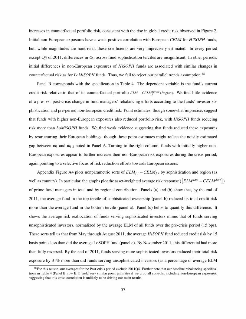
increases in counterfactual portfolio risk, consistent with the rise in global credit risk observed in Figure 2.
Initial non-European exposures have a weak positive correlation with European CELM for HiSOPH funds,
but, while magnitudes are nontrivial, these coefficients are very imprecisely estimated. In every period
except Q4 of 2011, differences in ωkt across fund sophistication terciles are insignificant. In other periods,
initial differences in non-European exposures of HiSOPH funds are associated with similar changes in
counterfactual risk as for LoMiSOPH funds. Thus, we fail to reject our parallel trends assumption.48
Panel B corresponds with the specification in Table 4. The dependent variable is the fund’s current
credit risk relative to that of its counterfactual portfolio ELM−CELMPeriodf (Region). We find little evidence
of a pre- vs. post-crisis change in fund managers’ rebalancing efforts according to the funds’ investor so-
phistication and pre-period non-European credit risk. Point estimates, though somewhat imprecise, suggest
that funds with higher non-European exposures also reduced portfolio risk, with HiSOPH funds reducing
risk more than LoMiSOPH funds. We find weak evidence suggesting that funds reduced these exposures
by restructuring their European holdings, though these point estimates might reflect the noisily estimated
gap between ω3 and ω1,2 noted in Panel A. Turning to the right column, funds with initially higher non-
European exposures appear to further increase their non-European risk exposures during the crisis period,
again pointing to a selective focus of risk reduction efforts towards European issuers.
Appendix Figure A4 plots nonparametric sorts of ELM f ,t −CELM f ,t by sophistication and region (as
well as country). In particular, the graphs plot the asset-weighted average risk response ([ELMdate−CELMdate
])
of prime fund managers in total and by regional contribution. Panels (a) and (b) show that, by the end of
2011, the average fund in the top tercile of sophisticated ownership (panel b) reduced its total credit risk
more than the average fund in the bottom tercile (panel a). Panel (c) helps to quantify this difference. It
shows the average risk reallocation of funds serving sophisticated investors minus that of funds serving
unsophisticated investors, normalized by the average ELM of all funds over the pre-crisis period (15 bps).
These sorts tell us that from May through August 2011, the average HiSOPH fund reduced credit risk by 15
basis points less than did the average LoSOPH fund (panel c). By November 2011, this differential had more
than fully reversed. By the end of 2011, funds serving more sophisticated investors reduced their total risk
exposure by 31% more than did funds serving unsophisticated investors (as a percentage of average ELM
48For this reason, our averages for the Post-crisis period exclude 2011Q4. Further note that our baseline rebalancing specifica-tions in Table 4 (Panel B, row B.1) yield very similar point estimates if we drop all controls, including non-European exposures,suggesting that this cross-correlation is unlikely to be driving our main results.
57

-35
-30
-25
-20
-15
-10
-5
0
5
10
May
-11
Jun-1
1
Jul-
11
Aug-1
1
Sep
-11
Oct
-11
Nov-1
1
Dec
-11
Jan-1
2
Feb
-12
Mar
-12
Apr-
12
May
-12
Jun-1
2
Jul-
12
Aug-1
2
Sep
-12
Oct
-12
Nov-1
2
Dec
-12
(a) All funds with low SOPH: Reallcoations by region
All
Europe
Americas
Asia/Pacific
Bps:
-35
-30
-25
-20
-15
-10
-5
0
5
10
May
-11
Jun-1
1
Jul-
11
Aug-1
1
Sep
-11
Oct
-11
Nov-1
1
Dec
-11
Jan-1
2
Feb
-12
Mar
-12
Apr-
12
May
-12
Jun-1
2
Jul-
12
Aug-1
2
Sep
-12
Oct
-12
Nov-1
2
Dec
-12
(b) All funds with high SOPH: Reallcoations by regionBps:
-60
-50
-40
-30
-20
-10
0
10
20
30
May
-11
Jun-1
1
Jul-
11
Aug-1
1
Sep
-11
Oct
-11
Nov-1
1
Dec
-11
Jan-1
2
Feb
-12
Mar
-12
Apr-
12
May
-12
Jun-1
2
Jul-
12
Aug-1
2
Sep
-12
Oct
-12
Nov-1
2
Dec
-12
(c) High SOPH - Low SOPH funds:
Reallocations by region, normalized by
average pre-period ELM
%Δ:
-15
-10
-5
0
5
May
-11
Jun-1
1
Jul-
11
Aug-1
1
Sep
-11
Oct
-11
Nov-1
1
Dec
-11
Jan-1
2
Feb
-12
Mar
-12
Apr-
12
May
-12
Jun-1
2
Jul-
12
Aug-1
2
Sep
-12
Oct
-12
Nov-1
2
Dec
-12
(d) All funds: Reallocations by issuer country
France Belgium Italy Germany
UK Canada Japan Aus/NZ
Bps:
Figure A4: Credit risk reallocations,[ELMdate−CELMdate (RegionorCountry)
]This figure shows the asset-weighted average of
[ELMdate−CELMdate (Region)
]across each group of prime MMFs. This is cal-
culated as the actual contribution of a given region to a fund’s credit risk on a given date minus the counterfactual contribution hadthe fund continued to hold the same securities it held as of May 31, 2011 (measured as basis point changes). Panel (a) (top left) in-cludes only those funds with ownership by sophisticated investors (SOPH) in the bottom tercile, while Panel (b) (top right) includesonly those funds with SOPH in the top tercile. The lines in Panel (c) (bottom left) are calculated as the average risk reallocation forall high SOPH funds minus the average risk reallocation for all low SOPH funds. We normalize these differences by the averagefund ELM for the pre period (15 bps). Panel d (bottom right) shows the asset-weighted average
[ELMdate−CELMdate (Country)
]across all prime MMFs. Omitted countries, such as the U.S., have an average risk response that is consistently very close to zero.
in May 2011). Risk reductions were entirely met from European investments. However, the average fund in
the top tercile of sophisticated ownership was more likely to offset part of the reduction with additional risk
58

from the Asia/Pacific region. The average fund withdrew most from French and Belgian issuers while risk
exposures to Japanese issuers grew the most (panel d).
In the main analysis, we quantify a manager’s rebalancing effort as the difference between her actual
portfolio risk – where “risk” is measured as ELM – and her counterfactual portfolio risk (had she maintained
her initial portfolio over time). Here, we explore a different approach which does not require specifying
such a counterfactual, though the basic design remains the same. Specifically, we evaluate three alternative
measures of portfolio rebalancing: (1) the number of issuers for all European securities, (2) the portfolio
weight allocated to European issuers, and (3) the weighted average maturity on European securities. We
separately evaluate these outcomes for all European securities, and uncollateralized European securities.
Uncollateralized securities have lower recovery rates and, hence, may be more information-sensitive.
Table A5 presents estimates of βk,t , based on the specification in Equation 2, for alternative measures
of rebalancing of funds’ European portfolios. Columns (1)–(3) provide estimates for the pre-crisis pe-
riod (January-April 2011), while columns (4)–(6) provide estimates for the post-crisis period, as defined
above. Consistent with our previous results, we find that the pre-period differences between HiSOPH and
LoMiSOPH funds are statistically indistinguishable for all dependent variables.
In the post-period, we observe economically and statistically significant differences by investor sophis-
tication in manager responses to initial portfolio risk. The first two rows use as dependent variables the
change in the number of issuers for all European securities and uncollateralized securities, respectively. The
first row of column (4) suggests that a HiSOPH fund drops a European issuer from its portfolio per 2.8 bps
in initial European exposure. Column (6) implies that, relative to a similar LoMiSOPH fund, a HiSOPH
fund rids an additional 1.5 European issuers from its portfolio per standard deviation in initial European
ELM (5 bps).
In the next two rows, we look at changes in the portfolio weight allocated to European issuers. Again,
we find negative and highly significant coefficients for both HiSOPH (column 4) and LoMiSOPH (column
5) funds. The difference is statistically significant at the 10% level (t-statistic of -2.0) only in the case of
uncollateralized holdings. Although the slope coefficients are similar in magnitude for the uncollateralized
securities, they are more precisely estimated, suggesting that the observed reductions in portfolio shares for
exposed funds are driven predominantly by the uncollateralized portion of the portfolio.
59

Table A5: Rebalancing - effect of sophistication and European exposure on other characteristics of Europeanholdings
These are monthly cross-sectional regressions across fund portfolios over the “Pre-crisis” (January–April 2011) and “Post-crisis”(2011Q4–2012Q3) periods. Reported coefficients are averages of monthly regression coefficients. Dependent variables measure (1)the number of European issuers that are financed by the fund, (2) the portfolio weight allocated to European securities, and (3) theweighted average number of days until maturity of securities originating from Europe. These dependent variables are demeaned foreach fund using the corresponding fund observation from May 31, 2011 and can, therefore, be interpreted as “changes since May2011.” Results are shown for the full set of securities and, separately, for the subsample of securities that are not fully collateralizedby U.S. government securities. The table reports coefficients on interactions of a fund’s average pre-period expected-loss-to-maturity from European securities, ELM(EU) f , with tercile dummies of low-to-mid sophistication, LoMiSOPH, and, separately,high sophistication (HiSOPH). Controls are as detailed in Table 3. Robust standard errors are shown in parentheses. Estimateswith a p-value below 0.10, 0.05, and 0.01 are marked with a *, **, and ***, respectively.
REBALANCINGPeriodf (Region) = αt +∑
3k=1
[βkELM(EU) f ×Dk f +ωkELM(NotEU) f ×Dk f
]+X ′f γ + ε f
Period: Pre-crisis Post-crisis
Coeff: [β3=Hi− [β3=Hi−β3=Hi β1,2=Lo,Mi β1,2=Lo,Mi] β3=Hi β1,2=Lo,Mi β1,2=Lo,Mi]
Dependent variable (Y f ) (1) (2) (3) (4) (5) (6)
∆# issuers financed by fund f 0.07 0.16 *** -0.09 -0.36 *** -0.07 -0.29 **
(0.53) (3.27) (-0.65) (-4.32) (-0.76) (-2.50)
uncollateralized version 0.09 0.13 *** -0.04 -0.32 *** -0.13 * -0.18
(0.67) (2.79) (-0.25) (-2.95) (-1.72) (-1.47)
∆Portfolio weight (% of AUM) 0.15 0.02 0.13 -1.58 *** -1.15 *** -0.43
(0.51) (0.12) (0.41) (-5.47) (-5.22) (-1.29)
uncollateralized version 0.07 0.21 -0.15 -1.64 *** -1.07 *** -0.57 **
(0.29) (1.62) (-0.57) (-6.19) (-6.55) (-2.00)
∆Weighted avg. maturity 0.32 0.34 -0.01 -0.59 -0.69 * 0.10
(1.00) (1.51) (-0.04) (-1.64) (-1.87) (0.20)
uncollateralized version 0.37 0.26 0.11 -1.28 ** -0.64 -0.63
(0.98) (0.87) (0.26) (-2.45) (-1.63) (-1.03)
Funds might alternatively have reduced their portfolio risk by reducing the maturity of their asset hold-
ings. The final two rows therefore repeat our analysis with the change in the fund’s weighted average matu-
rity, separately for all securities and uncollateralized securities. Point estimates are negative in all cases but
sharper for uncollateralized securities. For HiSOPH funds, we find that a one bp increase in initial European
exposure is associated with a statistically significant reduction in maturity of 1.3 days for uncollateralized
European holdings. While this magnitude is twice as large as the comparable coefficient for LoMiSOPH
funds, the difference between the two is not statistically significant.
60

Fund rebalancing and subsequent investor information acquisition-6
0-4
0-2
00
2040
Reg
ress
ion
coef
ficie
nt
Apr, 2011Jul, 2011
Oct, 2011Jan, 2012
Apr, 2012Jul, 2012
Month, year
ELM(EU) x LoMiSOPHELM(EU) x HiSOPH 95% CI
-60
-40
-20
020
40
Apr, 2011Jul, 2011
Oct, 2011Jan, 2012
Apr, 2012Jul, 2012
Month, year
ELM(NotEU) x LoMiSOPHELM(NotEU) x HiSOPH 95% CI
Figure A5: Investor information activity on SEC EDGAR website, by fund sophistication and European riskexposure (ELM)
The figure plots regression coefficients on interactions of a fund’s one-month lagged expected-loss-to-maturity from European andnot-European securities, ELM(EU) f ,t−1 and ELM(NotEU) f ,t−1, with tercile dummies of low-to-mid sophistication, LoMiSOPH,and, separately, high sophistication (HiSOPH). The dependent variable is the number of times a fund’s EDGAR page was viewedin month t per 10,000 accounts. Since funds serve different numbers of investors, which may mechanically boost or reduce pageviews relative to other funds, this variable is normalized by, first, dividing by the number of investor accounts in the fund and, then,by subtracting off the pre-crisis (January–May 2011) mean value of this amount, then multiplying by 10,000. In other words, thedependent variable is the difference in a fund’s average number of views per account per month relative to the fund’s pre-periodmonthly average. The dependent variable is winsorized at the 2nd and 98th percentile.
In the main text, we argue that managers reduce exposures to information-sensitive securities in order
to reduce the incentives for investors to monitor their portfolio holdings in future periods. Here, we provide
direct evidence consistent with this argument. Specifically, we use our measures of investor page views on
the EDGAR website, relative to the number of accounts, as a proxy for investor information acquisition and
test whether reductions in portfolio risk exposures are associated with differences in monitoring intensity.
61

Then, we use a regression almost identical to Equation (2), except that we use one-period lagged measures
of European and non-European ELM in place of initial ELM. Figure A5 plots monthly coefficients for
European ELM (β3 and 1/2β1+1/2β2) and non-European ELM (ω3 and 1/2ω1+1/2ω2) in panels A and B,
respectively. The web traffic measures are expressed in units of number of views per 10,000 accounts.
Prior to the start of the crisis, estimates of β3 and 1/2β1+1/2β2 are insignificantly different from one
another and slightly negative, consistent with investors not monitoring funds differentially according to
European risks prior to the start of the crisis. A negative coefficient could be expected if very large funds
(in terms of number of accounts) also tend to have higher European credit risk. This could occur if, for
example, there are economies of scale in purchasing securities from a larger number of foreign issuers. If
many of these accounts correspond with retail investors who do not engage in information acquisition, this
could imply that we have the wrong scaling factor in the denominator of the dependent variable. This creates
a downward bias in the coefficients which would work against us finding the positive relation noted above.
As the the crisis continues, consistent with the argument in Section 3, decreases in European ELM are
associated with statistically significant decreases in information acquisition activity for HiSOPH funds. In
contrast, declines in non-European ELM are not associated with changes in information acquisition activity
for HiSOPH funds, and coefficients remain modestly negative or insignificant for LoMiSOPH funds’ expo-
sures from both regions. In short, these results are consistent with the idea that managers of HiSOPH funds
are able to reduce investors’ monitoring intensity by reducing exposures to information-sensitive European
risks.
62

B Measuring Credit Risk
Construction of Expected-Loss-to-Maturity (ELM)
To evaluate the risk preferences of funds and their investors during the Eurozone crisis, we construct a
measure of credit risks in MMF portfolios. This is necessary because MMFs price their portfolio holdings
at amortized cost, such that fund yields (and yield spreads) do not immediately reflect changes in the credit
quality of their portfolios’ securities. Furthermore, current market yields on MMFs’ outstanding portfolio
securities are frequently unavailable, since secondary markets for short-term securities, like CDs and CP,
are notoriously thin (Covitz and Downing, 2007). Thus, to study credit risk in MMFs, we use a measure
that evolves with market conditions.
This appendix describes the approach used in this paper – which is based on a method proposed in
Collins and Gallagher (2016) – to estimate the credit risk of prime money market funds. For exposition, we
introduce the following notation:
I = total number of issuers in a fund’s portfolio
J = total number of securities in a fund’s portfolio
Tj = remaining days to maturity for security j
wi j = proportion of a fund’s assets invested in security j issued by issuer i
Ri = recovery rate on an issuer i’s securities in the event of a default
pi(Tj) = cumulative probability through time Tj that issuer i defaults; i.e., P(Di < Tj)
p̃i(Tj) = 1− [1− pi(Tj)]360/Tj , the annualized counterpart of pi(Tj)
Define expected loss-to-maturity (ELM) for a given fund at a given moment in time to be:
ELM =I
∑i=1
J
∑j=1
wi j(1−Ri)p̃i(Tj) (A1)
To make Equation (A1) operational, we use default probabilities provided by RMI, which are described
in Section 4.1. By hand, we match the month-end portfolio holdings of prime MMFs issuer-by-issuer and
maturity-by-maturity with default probabilities obtained from RMI. Given the RMI default probabilities, the
63

annualized expected loss on each security j issued by issuer i is simply (1−Ri)p̃i(Tj).49 In other words,
the expected loss on a security from a given issuer with a given remaining maturity is the relevant default
probability times the expected loss given default. ELM approximates the annualized expected loss on a
fund’s portfolio, where each security is multiplied by its portfolio weight, wi j. Thus, from expected losses
on individual portfolio securities, we can calculate the expected losses on individual prime MMFs, as in
Equation (A1), and on prime MMFs as a group (i.e., asset-weighted average ELM). We can also sum the
contribution to a fund’s total credit risk of securities issued by companies headquartered in a given region
(e.g., ELM (Europe) = ∑Ii=1 ∑
Jj=1 wi j(1−Ri)p̃i(Tj), where i ∈ Europe).
To calculate ELM we also need recovery rates, Ri, for each issuer. Consistent with market practice
(and with Collins and Gallagher, 2016), we use a recovery rate of .40 for all private sector issuers except
Japanese banks. For Japanese banks, we follow market convention and use a recovery rate of .35. Prior
research suggests that the added complexity of randomizing recovery rates may not offer much additional
insight. Tarashev and Zhu (2008) indicate, based on data collected from Markit for 136 entities, that the
recovery rate that market participants expect varies in a narrow range around 40 percent for daily data from
late 2003 to early 2005. Consequently, we fix our recovery rates at either .35 or .4, depending on the parent
company. If our chosen recovery rates reasonably approximate market views, a fund’s ELM should be a
close, leading indicator of its gross yield spread, which is indeed the case.
We are able to match default probabilities from RMI with the list of parent firms collected from the
N-MFP reports for over 90% of the assets of prime MMFs (excluding, from the denominator, assets issued
by the U.S. government). Here we explain our strategy for handling the 10% of assets that could not be
matched to an RMI default probability and the assumptions we make about the appropriate recovery rates
and default probabilities to assign to certain security types.
• The fixed income securities MMFs hold sometimes have credit enhancements, such as a guarantee,letter of credit, or other provision that guarantees return of principal and interest. Although suchenhancements reduce the risk of holding a security, we do not take them into account, except in caseswhere the guarantee is provided by the U.S. government or other sovereign nation, in which cases weset Ri = 1.
49To make Equation (A1) operational, we linearly interpolate default probabilities for every day between the maturities that RMIprovides. Because some of the securities held by prime funds mature within 1 to 7 days (e.g., overnight repurchase agreements), wealso need estimates of default probabilities for maturities of less than 1 month. We solve this problem by ruling out the possibilityof instantaneous default (i.e., p̃i(Tj = 0) = 0), allowing us to linearly interpolate between that value and p̃i(Tj = 30,360). Throughthis process we obtain p̃i(Tj) for any intervening maturity.
64

• One exception to the above rule is when the security is a Variable Rate Demand Note (VRDN) issuedby a company that is not in the RMI database. For example, if Akron Hardware issues a VRDNwith a demand feature provided by Bank of America, we would apply Bank of America’s probabilityof default before maturity (with the maturity set to the next put date). About 3% of fund assets arematched to default probabilities following this method.
• MMFs sometimes hold asset-backed securities. All else equal, asset-backed commercial paper (ABCP)have less credit risk than securities that are not asset-backed. For example, recovery rates on asset-backed securities that defaulted during the 2007-2008 crisis are generally reported to have been muchhigher (in the range of 80 percent or more) compared with a recovery rate of about 40 percent onunsecured Lehman Brothers debt. Thus, for ABCP, we set Ri = 0.80.
• Repurchase agreements (repo) are more than fully collateralized by securities that a fund’s repo coun-terparty (the borrower) must place with a third-party custodian. All else equal, this makes repo lessrisky than other senior unsecured debt. Thus, we we set Ri = 0.80 for repo unless the repo is fullycollateralized by Treasury and agency securities, in which case we treat repo as having the default riskof the U.S. government (i.e., Ri = 1).
• About 5% of fund holdings are issued by municipalities (for which RMI does not calculate defaultprobabilities). These are most often in the form of VRDNs, which typically have 1-day or 7-daydemand features. These securities are generally considered to be of high credit quality since the fundcan tender the securities to the demand feature provider (usually a financial institution). Rather thanomit these securities from our analysis, we calculate the municipal-to-government money market fundspread on each day and assume the expected loss on a municipal security on a given day equals thisspread.
• To calculate an expected loss for the remaining 2% of assets that we cannot match with default prob-abilities, we use the average default probability of the security’s closest peer group. Peer groups arecomprised of securities with a similar maturity that are issued by other companies within the samesector and region.
• RMI does not publish default probabilities for sovereigns. Consequently, we assume that the defaultprobabilities for U.S. Treasury and agency securities are zero at all maturities.
As a final note, Collins and Gallagher (2016) explain why the above simplifying assumptions cannot be
avoided by using the yield and/or CUSIP detail available for each security on Form N-MFP to infer a fund’s
credit risk: “The yields on individual securities are usually reported as of the date of purchase, not the date
of filing. Thus, an aggregate credit risk measure based on reported security-level yields would lag behind
the current market. This issue cannot generally be overcome by using the CUSIPs listed on Form N-MFP
and linking those with current market yields from an outside data provider. The majority of prime MMF
assets are CP and CDs, for which in many cases price quotes are not readily available from data services
such as Bloomberg. Even if secondary markets were deeper, 24% of prime MMF assets do not have CUSIPs
reported on Form N-MFP, as of May 2011. Even more troublesome, funds often enter their own internal
65

CUSIPs on the Form, introducing matching error. Therefore, current market yields are unavailable for the
majority of holdings.” ELM overcomes these deficiencies.
Accuracy of RMI’s Default Probabilities
Our ELM measure uses default probability estimates computed by the Credit Research Initiative at the
National University of Singapore Risk Management Institute (RMI) and so we next provide details on the
predictive performance of the RMI default probability estimates. Further, we explain how cross-sectional
correlations in these probabilities is accounted for by their approach.50 The RMI has evaluated the accuracy
and unbiasedness of the default probability estimates in a series of technical reports as well as in published
academic research papers (e.g., Duan et al., 2012; Duan and Miao, 2016). In line with common practice
at financial institutions, the RMI measures model performance using accuracy ratios and by comparing
predicted and realized default rates on diversified portfolios with large numbers of assets. In NUS-RMI
(2017), prediction accuracy is evaluated using the accuracy ratio which is a statistic whose range is [0,1],
with zero representing a completely random rating and one representing a perfect rating. Accuracy ratios
are generally very high for European countries, e.g., in excess of 87% on average (across countries) at the
one-month horizon, including 85-87% accuracy ratios for France, Germany and Italy. The corresponding
figure for North America is 94%. Accuracy ratios are a bit lower at the one-year horizon, e.g., 75% for
Europe and 83% for North America. Prediction accuracy is also evaluated using a test statistic based on the
Area Under the Receiver Operating Characteristic (AUROC) which is commonly used in the literature on
evaluation of forecasts of binary data. For Europe as a whole, this measure (which equals one-half if there is
no genuine predictability of defaults) equals 0.94 at the one-month horizon and 0.88 at the one-year horizon.
Turning to the methodology used by the RMI model, forecasts of the probability of default (PD) are
based on the forward intensity model developed in Duan et al. (2012). In broad terms, correlations between
default probabilities are introduced into the RMI model both directly through the use of common covariates
and indirectly via individual firm attributes which, for many of the variables, are strongly correlated.
Specifically, the RMI default prediction system uses 16 market and accounting covariates tracking firm-
level characteristics, Yit , and macro-financial risk factors, Xt , to compute the conditional default probability
of firm i at time t for some forward period τ: pi,t(τ) = Pτ(Xt ,Yit). A key indicator of individual firms’ default
50We thank Professor Jin-Chuan Duan for answering our questions about the methodology and practices used by the RMI.
66

probabilities is the distance to default computed using a Merton-type structural model which assumes that
firms’ asset values follow geometric Brownian motion processes. Besides the distance to default, other firm-
specific attributes include idiosyncratic volatility (computed using a one-year horizon), relative size, net
income over total assets, and current assets over current liabilities. Some of these firm-specific attributes,
such as the idiosyncratic volatility, may themselves have a common factor structure and so can help to
incorporate cross-sectional correlations in default risks.
Macro-financial factors include the stock index return, a short interest rate, and the economy-level dis-
tance to default for financial and non-financial firms. The distance to default measures depend on aggregate
market volatility and so help capture correlations in default probabilities. In particular, these common fac-
tors will have contributed towards raising the default probabilities of the vast majority of firms during this
Eurozone Crisis.
The RMI model also incorporates cross-sectional dependencies in default probabilities through a second
channel. The parameters of the forward intensity model are estimated and updated each month using a set of
six calibration groups (North America, Europe, Asia-Developed economies, Emerging Markets, China, and
India). Parameter estimates are pooled for all companies in the same calibration group – for example, for
each firm the distance to default is computed using sector averages of debt computed as current liabilities,
plus half of long-term debt plus some sector-level average coefficient times other liabilities.
The RMI is careful in dealing with illiquidity, tossing out stocks with stagnant price series and adjusting
the distance to default in the Merton model accordingly. To handle issues related to maturities, the RMI uses
the Nelson-Siegel term structure model and sequential Monte Carlo estimation methods. The parameters of
the model only require end-of-month data although the daily estimates of the default probabilities require
daily updates of the firm-specific and aggregate covariates. For some variables, this is accomplished by
using rolling-window averages. More broadly, the pooling of parameter estimates mentioned above means
that not every asset needs to have an observation every day and so provides an effective way to deal with
illiquid assets.
67

Adjusting for Correlated Defaults Across Issuers
As discussed above, RMI’s default probabilities take into account the prospect of common shocks across
firms. As a further robustness test, it may be informative, however, to account for the extent of co-movement
in default probabilities across firms held within an individual fund’s portfolio. To do this, we borrow a
measure of the risk premium associated with a fund “breaking the buck” from Collins and Gallagher (2016).
In particular, this measure, BDI(50,300), stands for break the dollar insurance cost, allowing for an insurance
deductible of 50 bps and a maximum payout of 300 bps (consistent with the structure of the U.S. Treasury’s
2008–2009 temporary guarantee program for MMFs).
The advantage of BDI is that, to correctly assess the probability that a fund might break-the-buck,
default correlations are taken into account. This is done using a copula (Li, 2000) implemented by Monte
Carlo simulation. The approach involves simulating random default times for each issuer i a large number
of times, n = 1, ...,N. Default probabilities, and hence the random default times, are correlated across
issuers. Correlations are calibrated to historical movements in default probabilities from January 2011 to
December 2012 and this positive dependence is modeled using a t-copula. If a given simulation indicates
that issuer i defaults before time Tj, a fund experiences a loss on security j equal to the security’s portfolio
weight in the fund multiplied by the expected loss given default. Losses across all of a fund’s securities are
accumulated during a particular simulation, n. If a fund’s losses in simulation n accumulate to more than the
deductible (i.e., 50 basis points of the fund’s assets), the fund is counted as having broken the buck. Monte
Carlo methods are used to implement this process by sampling uniform random variates with a probability
of default based on the correlated default probabilities. The result is BDI – an estimate of the annualized
insurance premium needed to insure a fund against breaking the buck.
A disadvantage of BDI, and the reason we do not use it in the main paper, is that BDI cannot be directly
calculated on the basis of regional exposures (because it considers defaults to be correlated across all issuers,
even those from different regions, in a fund’s portfolio). In contrast, ELM can be generated on a regional
basis. Recall, ELM is just the weighted sum of the expected losses on the fund’s portfolio securities. Sums
can be performed on just the securities from a given region. This is why we use ELM and not BDI in our
main analysis. To try to use BDI to evaluate regional risk allocations, one must first regress BDI, at the fund-
date level, on an interaction between funds’ regional asset exposures and regional average CDS premiums.
68

Then, one can use the model to predict the effect on BDI of a fund’s asset exposures to particular regions at
a given moment in time.
Figure B1: Fund ELM and BDI over time, asset-weighted average
This figure plots the asset-weighted average value of ELM against the corresponding value of BDI(50,300) – which is an estimateof the annualized insurance premium needed to insure a fund against breaking the buck, with a 50 basis point deductible and a 300basis point maximum payout – over the 2011 through 2012 period.
Figure B1 below plots the overall (non-region specific) ELM and BDI measures for the asset-weighted
average fund. The two risk measures are clearly strongly correlated with a correlation of 0.95 for the asset-
weighted average fund over time and 0.85 across individual funds over time.
Figure B2 documents the robustness of our main results to using this alternative measure of credit
risk that accounts for correlated default probabilities within a fund. To construct this figure, we separately
predict BDI for low and high sophistication funds. Then, we plot the asset-weighted average predicted
value of BDI, by sophistication group, based on individual funds’ actual portfolio holdings as well as their
counterfactual (May 2011) portfolios. We do this for funds’ European (top panel) and Asia/Pacific (bottom
panel) exposures. Consistent with our paper’s key result based on ELM (presented in Table 4, Figure 7, and
Appendix Figure A4), we find that funds serving more sophisticated investors (RHS) rebalanced portfolio
risk out of Europe and into Asia on a larger scale than funds serving less sophisticated investors (LHS). Less
69
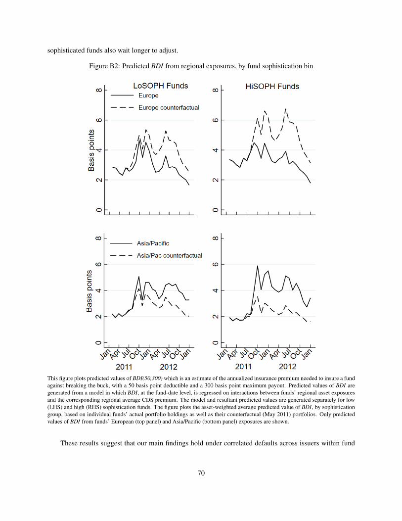
sophisticated funds also wait longer to adjust.
Figure B2: Predicted BDI from regional exposures, by fund sophistication bin
This figure plots predicted values of BDI(50,300) which is an estimate of the annualized insurance premium needed to insure a fundagainst breaking the buck, with a 50 basis point deductible and a 300 basis point maximum payout. Predicted values of BDI aregenerated from a model in which BDI, at the fund-date level, is regressed on interactions between funds’ regional asset exposuresand the corresponding regional average CDS premium. The model and resultant predicted values are generated separately for low(LHS) and high (RHS) sophistication funds. The figure plots the asset-weighted average predicted value of BDI, by sophisticationgroup, based on individual funds’ actual portfolio holdings as well as their counterfactual (May 2011) portfolios. Only predictedvalues of BDI from funds’ European (top panel) and Asia/Pacific (bottom panel) exposures are shown.
These results suggest that our main findings hold under correlated defaults across issuers within fund
70

portfolios.
71

C Investor Sophistication Measure (SOPH)
Our study attempts to precisely separate truly institutional investors (those whom act as an investment agent
for a principal that is not a natural person) from truly retail investors (including those whom invest through
a large 401(k) plan or through an omnibus brokerage account). To achieve this, we segregate high-level
investor types by whether they are predominantly institutional or retail in origin. For example, we have
data on fund ownership by financial corporations, nonfinancial corporations, retirement plans, retail broker-
directed accounts, and retail self-directed accounts.
The mutual fund industry and its transfer agents use what are called social codes to categorize share-
holder types. These social codes classify different types of investor accounts, such as 529 college savings
plans and defined benefit retirement accounts. Different transfer agents have different classification schemes,
thus, the data coming to the ICI (through fund companies) from the transfer agents is modified in order to
fit a unified classification system. The final data set tells us that the high-level category of fiduciary ac-
counts consists of subcategories, such as estates and inheritance trusts. Although we only know aggregate
shareclass assets in the higher-level categories (e.g., retirement plans), knowledge of the underlying subcate-
gories (e.g., 401(k) accounts) and conversations with industry experts about the dominant types of investors
who use MMFs guide our process of separating high-level shareholder types into either truly institutional or
retail.
In fact, a similar process of segregating institutions from retail investors is playing out across the MMF
industry, as fund companies seek to comply with the SEC’s 2014 reforms. Industry convention (based on
SEC suggestion) is to determine whether the investors within each social code are likely to have social
security numbers. If so, these investors are to be classified as “retail.” For example, the agent making the
investment decision for a 401(k) account is likely to be acting for principals having social security numbers,
while one investing on behalf of a defined benefit pension plan is likely to be acting for a principal that does
not have a social security number. Our classifications follow this guiding principle.
We define shares held by these investor types as being truly institutional (i.e., “sophisticated”) in na-
ture: nonfinancial companies, financial companies, nonprofits, state and local governments, other funds,
and other institutions.51 Within these six categories, the vast majority of assets come from financial and
51“Other institutions” are generally international organizations, unions, and cemeteries. The "other funds" category typically
72

Figure C1: Prime MMF shareholder-types
This figure shows the portion of aggregate assets of prime MMFs owned by different types of investors and the distribution ofinvestor sophistication (SOPH) across prime MMFs. “Other institutions” includes other intermediated funds (e.g., hedge funds andfund-of-fund mutual funds), state/local governments, and other types of institutions (e.g., international organizations, unions, andcemeteries). “Individuals” includes about equal proportions of individual-directed retail accounts and pooled brokerage omnibusaccounts. “Plans and trusts” are primarily fiduciary accounts (e.g., estates and inheritance trusts) and retirement plans (e.g., 401(k)and defined benefit pension plans) along with a small amounts from College 529 Savings Plans.
(a) The portion of aggregate assets of prime MMFs owned by different types of investors
Nonfinancials
19%
Financials
12%
Nonprofits
2%
Other
institutions
2%
Plans and
trusts
25%
Individuals
40%
Sophisticated investors: 34%
All share classes
Nonfinancials
28%
Financials
18%
Nonprofits
3%
Other institutions
3%
Plans and
trusts
23%
Individuals
25%
Sophisticated investors: 52%
Institutional share classes
(b) The distribution of investor sophistication (SOPH) across prime MMFs
69%
13%
7%5%
8%
38%
16%13%
8%
25%
0%
10%
20%
30%
40%
50%
60%
70%
80%
0-20% >20-40% >40-60% >60-80% >80-100%
Per
cen
tag
e o
f ca
teg
ory
Ownership by sophisticated investors
All funds
Institutional share classes
accounts for less than 1% of prime MMF assets. We classify these accounts as institutional because an unknown, but presumablydominant, share comes from hedge funds.
73

nonfinancial companies, which are clearly truly institutional. Our retail (i.e., “unsophisticated”) categories
include: retirement plans, 529 plans, fiduciary accounts, brokers dealer/omnibus accounts, and individual
investor accounts. While these categorizations may not be perfect, we believe that this approach produces
the lowest asset misclassification. Throughout our analysis, we measure investor sophistication, SOPH, as
the portion of truly institutional investors, as defined above, in a given fund or shareclass. As documented
in Figure C1a, a significant fraction of AUM in institutional classes originates from natural persons: 25% is
held by individuals through retail accounts or through brokers, and another 23% held by trusts and retire-
ment plans for individual investors. Figure C1b also illustrates that there is large cross-sectional variation
in the share of total “truly institutional” ownership (i.e., SOPH) across MMFs. About 42% of shareclasses
have very little or no institutional ownership. On the other hand, 16% of institutional shareclasses are almost
entirely owned by true institutions. We verify that the underlying composition of investor types, at least in
aggregate, have not changed substantially through time.
This dataset has one important limitation. The ICI aggregates the data collected from fund companies,
which receive the data from transfer agents. Transfer agents often charge funds to return information on
the types of shareholders in their funds. Therefore, in any given year, a fund may choose not to acquire
such data. When a fund does not provide data at the end of a particular year, the ICI estimates its responses
by interpolating between prior and future responses or, until a future response is available, using the prior
response. In the rare instance of when a fund has never reported, the ICI estimates the assets belonging
to each shareholder-type in each shareclass of the fund based on responses from the funds’ peer group
(matched based on method of sale, name, size, and expense ratio). As of 2011, the survey captures 95% of
prime MMF dollar assets and 81% of shareclasses, by number, excluding estimates. Hence, it is typically
small funds that, on occasion, do not respond to the survey. Once these estimates are incorporated, 100% of
dollar assets and numbers of shareclasses are represented.
Our study uses the full data set, including estimates. We do this for two reasons. First, after omitting
estimates, we find that investor make-up changes very little over time, meaning the ICI’s estimates are likely
to be computed consistently over time. Second, our study seeks to describe large dollar responses on the
part of funds and their investors – the kind that may be relevant for systemic risk purposes. A degree of
measurement error in the classification of small funds is unlikely to affect results. Indeed, when we remove
74

designated estimates (representing 5% of assets) all results qualitatively hold. Despite its limitations, we
believe this to be the best data set in existence on MMF shareholders.
75

D SEC EDGAR Page Views
SEC EDGAR Information Acquisition Measures
This section describes the steps required to construct our measure of investor information acquisition from
the SEC’s EDGAR website. We use the following sequence of steps to collect and process the data.
1. We download the flat files for the 2011-2012 period from https://www.sec.gov/dera/data/edgar-log-file-data-set.html, which has a single file for each calendar day. This dataset alsoincludes the url (accession) associated with each individual page view, a scrambled IP address of theuser, as well as a detailed time stamp.
2. From the ICI, we obtain the EDGAR Central Index Key (CIK) and series ID associated with eachMMF. We discard any page which is not associated with the filings of a MMF. There is also a thirdidentifier, the Class/contract id which is associated with each individual shareclass.
3. Often the CIK is related to the fund management company, rather than a single MMF. For example,CIK 276516 is the Fidelity Money Market Trust, which is associated with two different funds: theRetirement Government Money Market Portfolio (series id S000007116) and the Retirement Gov-ernment Money Market II Portfolio (series id S000007117). Accordingly, this CIK has two differentN-MFP forms filed each month. However, each filing includes a table which lists the CIK, series ID,and class/contract IDs associated with each form, which looks like this:
We write a simple scraping algorithm to extract the associated information. This allows us to associateeach specific filing with a given set of funds (series IDs).
4. Next, we use the cleaned information from the WRDS SEC Analytics Suite to get the type of formwhich is associated with each individual filing. This allows us to isolate page views which are as-
76

sociated with specific forms. We aggregate page views associated with the holdings reports (FormN-MFP, and associated amended versions) and summary prospectuses (Form 497K), which are filedat the series ID level.52
5. Following Loughran and Mcdonald (2014), we impose a “no robot” filter, excluding IP addresseswhich visit more than 50 CIKs on a given day. Finally, to compute the measure of informationacquisition, we count the number of page views associated with a given fund over various intervals oftime. For Figure 5, these views are divided by the total number of accounts (from the ICI) associatedwith funds in each sophistication bin, then multiplied by 10,000. For the regressions in Table A5,these traffic measures are instead normalized by the number of accounts in each fund.
6. For the subset of IP addresses which pass the “no robot” filter, we compute a measure of overallactivity on the EDGAR site. For Figure 5B, we compute the average number of monthly page viewsassociated with CIKs which are linked with at least one MMF, then rank IP addresses into tercilesbased on this measure.
Bloomberg News Coverage Measures
Figure 3 plots a measure of the number of monthly news articles associated with issuers in different regions
over time. To do this, we begin by constructing a list of unique issuers which are used in the regressions in
Section 7, which we then hand match to ticker symbols in the Bloomberg database. We extract time series
on the number of news articles (NEWS_HEAT_PUB_DNUMSTORIES) which are associated (tagged) with
each ticker on each calendar date from 2010-2012. To do so, we follow a procedure virtually identical to the
one described in the internet appendix of Ben-Rephael et al. (2017) utilizing the Bloomberg Excel add-in.
To aggregate across issuers, we compute a weighted average of these news measures, using the the
dollar value of outstanding securities as of the end of May 2011 of each issuer within each region as weights.
This gives us monthly time series of news coverage associated with issuers in each region. We normalize
these indices so that the average monthly volume of articles in 2010 corresponds with a value of 100.
52In a small handful of cases, a particular CIK/series ID is associated with multiple funds. In these situations, we allocate trafficfrom these filings proportionally to dollar volume.
77
Top Related