


Languages
Pages
Legal

University of Twente
Master Thesis
Investigation of Infragravity Waves in aTwo-dimensional Domain using anon-hydrostatic numerical model,
SWASH
Author:
Nikolaos Alavantas
Supervisor:
Dr. ir. Jan S. Ribberink
Dr.ir. Bas Borsje
Ir. Matthijs Benit
Dr. ir. Gerbrant Ph. van
Vledder
A thesis submitted in fulfillment of the requirements
for the degree of Master of Science
in the
Civil Engineering and Management
In collaboration with:
April 2015

Declaration of Authorship
I, Nikolaos Alavantas, declare that this thesis titled, ’Investigation of Infragravity
Waves in a Two-dimensional Domain using a non-hydrostatic numerical model, SWASH’
and the work presented in it are my own. I confirm that:
� This work was done wholly or mainly while in candidature for a research degree
at this University.
� Where any part of this thesis has previously been submitted for a degree or any
other qualification at this University or any other institution, this has been clearly
stated.
� Where I have consulted the published work of others, this is always clearly at-
tributed.
� Where I have quoted from the work of others, the source is always given. With
the exception of such quotations, this thesis is entirely my own work.
� I have acknowledged all main sources of help.
� Where the thesis is based on work done by myself jointly with others, I have made
clear exactly what was done by others and what I have contributed myself.
Signed:
Date:
i

ii
Aknowledgements
1. There are no words in English or in Greek to thank you enough Katerinio.
2. I would like to address special thanks to my daily supervisor , Ir. Matthijs Benit
for his personableness, support, advice and endless patience in improving my mod-
elling skills.
3. Besides my daily supervisor, I would like to thank the rest of my thesis committee:
Dr. ir Jan Ribberink and Dr. ir. Bas Borsje.
4. I thank my fellow colleagues in ARCAIDS : Rodrigo Concalves, Robbin van Santen
and Jurjen Wilms , for the stimulating discussions and for all the fun we have had
in the last seven months. In particular, I am grateful to Martin van der Wel for
enlightening me the first glance of research.
5. I would like to express my gratitude to Dr. ir. Gerbrant Ph. van Vledder for his
guidance and help in the achievement of this work.
6. I would like to thank Dr. Zeki demirbilek, Ir. Anouk de Bakker and Dr. ir. Marcel
Zijlema for providing me insightful comments support and very useful materials.

UNIVERSITY OF TWENTE
Abstract
Civil Engineering and Management
Master of Science
Investigation of Infagravity Waves in a Two-Dimensional Domain
by Nikolaos Alavantas
Infragravity waves (IG) are generated due to the non-linear interactions between the
short (in terms of length) waves. IG waves propagate bounded to the short wave groups
and they are released when fluctuations to the short wave energy occur. Aim of this
research is to determine the behavior of IG waves around and inside the two-dimensional
domain of Barbers Point Harbour on the island of Oahu, Hawaii, USA. In order to achieve
simulation of IG waves, an extensive investigation is taking place, aiming to propose the
most accurate numerical wave model for the particular case. The conclusion is that an
efficient simulation of the harbour domain needs the usage of a phase-resolving and non-
linear wave model, SWASH. SWASH showed consistency for the IG wave calculation
(inside the basin of Barbers Point harbour) and its predictive skill measured approxi-
mately 0.84. Finally a further analysis is taking place, in order to decompose the IG
signal. Aim is to separate the IG waves to free and bounded by using bispectral analysis
and the separation method proposed by Sheremet et al. [2002]. The results are presented
for the area outside the harbour. IG waves seem to be generated 500m seawards of the
inlet. Additionally, the shore is identified as partially reflective boundary, even for the
IG waves (R2IG = 0.6). Finally, the behavior of the IG waves are affected by the entrance
channel. IG waves (as long waves) are strongly refracted by the channel and continue
to propagate inside the basin, when the short waves follow another path, leading to the
adjacent shores.
Keywords: infragravity waves, modeling, SWASH, bispectral analysis, free IG waves,
bound IG waves

iv
Phase: fraction of wave cycle which has elapsed relative to the origin.
Turbulent energy: the mean kinetic energy per unit mass associated with eddies in
turbulent flow.
Phase speed: the rate at which the phase of the wave propagates in space.
Shoaling: the effect by which surface waves entering shallower water increase in wave
height. Wave speed and length decrease in shallow water, therefore the wave energy
increases, so the wave height increases.
Refraction: is the change in direction of a wave due to a change in topography. Part
of the wave is in shallower water and as a result is moving slower compared to the part
in deeper water. So, the wave tends to bend when the depth under the crest varies.
Diffraction: is the change in direction of a wave due to an surface-piercing obstacle.
Waves turn into the region behind the obstacle and carry wave energy and the wave
crest into the ”shadow zone”. The tunning of the waves into the sheltered area is caused
by the changes in the wave height, in the same wave.
Resonance: the tendency of a system to oscillate with greater amplitude at some fre-
quencies than at others.
Vorticity: is a vector field that gives a microscopic measure of the fluid rotation at any
point (the tendency of something to rotate).
Quadratic: is describing a second order relationship
Harmonics: is a component frequency of the wave signal.
Langarian velocity: the distance a water particle travels in one wave period, divided
by that period.
Eulerian velocity: the short-wave-averaged velocity observed at a fixed point.
Dimensionless depth: Water depth, d, multiplied by the wave number, k.
Forchheimer dissipative terms: are developed for the macroscopic momentum and
energy balance equations considering saturated thermoelastic porous media, and for the
macroscopic momentum balance equations in the case of multiphase porous media.
Linear field: The area where the superposition principle can be applied. The net
displacement of the medium at any point in space or time, is simply the sum of the
individual (sine and cosine) wave displacements. In most of the cases, linear fields are
located in deep or shallow waters.
Cos-spectrum: The cross-correlation between two time series as a function of fre-
quency primar short wave frequency components
Primar frequency components: Frequency components where most of the energy is
concentrated
Contents
Declaration of Authorship i
Aknowledgements ii
Abstract iii
Definitions iv
Contents v
List of Figures viii
List of Tables xii
Abbreviations xiii
1 Introduction 1
1.1 Background . . . . . . . . . . . . . . . . . . . . . . . . . . . . . . . . . . . 1
1.2 Motivation . . . . . . . . . . . . . . . . . . . . . . . . . . . . . . . . . . . 2
1.3 Research question . . . . . . . . . . . . . . . . . . . . . . . . . . . . . . . . 3
1.4 Objectives . . . . . . . . . . . . . . . . . . . . . . . . . . . . . . . . . . . . 3
1.5 Thesis outline . . . . . . . . . . . . . . . . . . . . . . . . . . . . . . . . . . 5
2 Infragravity waves 6
2.1 Generation and propagation . . . . . . . . . . . . . . . . . . . . . . . . . . 6
2.2 Incident free long waves . . . . . . . . . . . . . . . . . . . . . . . . . . . . 8
2.3 Reflected infragravity waves . . . . . . . . . . . . . . . . . . . . . . . . . . 10
2.4 Dissipation mechanisms . . . . . . . . . . . . . . . . . . . . . . . . . . . . 13
3 Numerical modeling and IG analysis 16
3.1 SWASH . . . . . . . . . . . . . . . . . . . . . . . . . . . . . . . . . . . . . 18
3.1.1 Fundamental equations . . . . . . . . . . . . . . . . . . . . . . . . 18
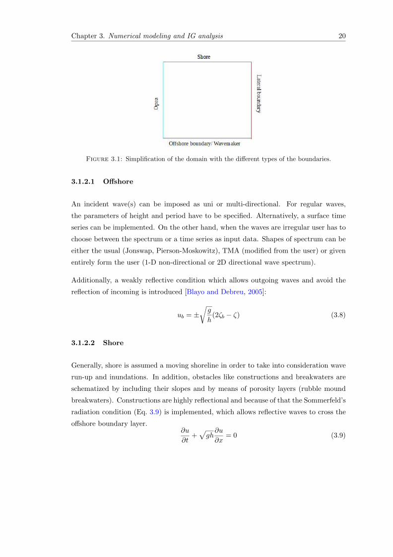
3.1.2 Boundary conditions . . . . . . . . . . . . . . . . . . . . . . . . . . 19
3.1.2.1 Offshore . . . . . . . . . . . . . . . . . . . . . . . . . . . . 20
3.1.2.2 Shore . . . . . . . . . . . . . . . . . . . . . . . . . . . . . 20
3.1.2.3 Lateral boundary . . . . . . . . . . . . . . . . . . . . . . 21
v

Contents vi
3.1.3 Wave breaking . . . . . . . . . . . . . . . . . . . . . . . . . . . . . 21
3.2 Post data analysis and the decomposition of IG waves . . . . . . . . . . . 21
3.3 Evaluation of SWASH . . . . . . . . . . . . . . . . . . . . . . . . . . . . . 24
3.4 Conclusion . . . . . . . . . . . . . . . . . . . . . . . . . . . . . . . . . . . 26
4 The two-dimensional case: Barbers Point Harbour 27
4.1 Instrumentation . . . . . . . . . . . . . . . . . . . . . . . . . . . . . . . . . 28
4.2 Wave measurements . . . . . . . . . . . . . . . . . . . . . . . . . . . . . . 29
4.3 Other characteristics of the harbour . . . . . . . . . . . . . . . . . . . . . 30
4.4 Infragravity wave regime . . . . . . . . . . . . . . . . . . . . . . . . . . . . 31
4.5 Model setup . . . . . . . . . . . . . . . . . . . . . . . . . . . . . . . . . . . 32
4.5.1 Offshore wave conditions . . . . . . . . . . . . . . . . . . . . . . . . 33
4.5.2 Lateral boundaries . . . . . . . . . . . . . . . . . . . . . . . . . . . 33
4.5.3 Other input parameters . . . . . . . . . . . . . . . . . . . . . . . . 34
5 Sensitivity analysis and model validation 36
5.1 Sensitivity Analysis . . . . . . . . . . . . . . . . . . . . . . . . . . . . . . . 36
5.1.1 Directional spreading . . . . . . . . . . . . . . . . . . . . . . . . . . 37
5.1.2 Sponge layers . . . . . . . . . . . . . . . . . . . . . . . . . . . . . . 39
5.1.3 Grid size . . . . . . . . . . . . . . . . . . . . . . . . . . . . . . . . 40
5.1.4 Vertical layers . . . . . . . . . . . . . . . . . . . . . . . . . . . . . . 41
5.1.5 Breaking parameter . . . . . . . . . . . . . . . . . . . . . . . . . . 42
5.2 IG wave inside the basin . . . . . . . . . . . . . . . . . . . . . . . . . . . . 43
5.3 Predictive skill of SWASH . . . . . . . . . . . . . . . . . . . . . . . . . . . 43
6 Separation of the Infragravity waves 46
6.1 Methodology . . . . . . . . . . . . . . . . . . . . . . . . . . . . . . . . . . 46
6.1.1 Description of the domain and the wave conditions . . . . . . . . . 46
6.1.2 Analysis . . . . . . . . . . . . . . . . . . . . . . . . . . . . . . . . . 48
6.2 Results . . . . . . . . . . . . . . . . . . . . . . . . . . . . . . . . . . . . . . 49
6.2.1 Separation of the total signal . . . . . . . . . . . . . . . . . . . . . 49
6.2.2 Decomposition of IG waves . . . . . . . . . . . . . . . . . . . . . . 50
6.2.3 Reflection analysis . . . . . . . . . . . . . . . . . . . . . . . . . . . 53
6.3 Discussion . . . . . . . . . . . . . . . . . . . . . . . . . . . . . . . . . . . . 56
6.3.1 Decomposition of the wave signal and the energy transmission . . 56
6.3.2 Bispectral analysis . . . . . . . . . . . . . . . . . . . . . . . . . . . 57
6.3.3 The reflection analysis . . . . . . . . . . . . . . . . . . . . . . . . . 58
7 Conclusion 60
7.1 Answering the research questions . . . . . . . . . . . . . . . . . . . . . . . 60
7.2 Recommendations . . . . . . . . . . . . . . . . . . . . . . . . . . . . . . . 62
A Background knowledge 64
A.1 Hilbert transformation . . . . . . . . . . . . . . . . . . . . . . . . . . . . . 64
A.2 Cross-correlation . . . . . . . . . . . . . . . . . . . . . . . . . . . . . . . . 64
A.3 Breaking criterion . . . . . . . . . . . . . . . . . . . . . . . . . . . . . . . 65

Contents vii
B Sensitivity analysis and results for the S17 storm 66
C Amplification factors for the Barbers Point harbour 68
D Breaking Zones 71
E Directional spectra 73
F Bispectra analysis for the PIn profile 82
Bibliography 85
List of Figures
1.1 Energy spectrum for different types of waves[Munk, 1950]. . . . . . . . . . 1
1.2 Short waves (solid line) travel in groups, and together they induce aninfragravity wave (dashed line). . . . . . . . . . . . . . . . . . . . . . . . . 2
2.1 Spectral evolution as a friction of the cross-shore position (x) and thefrequency (f) [Michallet et al., 2014] . . . . . . . . . . . . . . . . . . . . . 7
2.2 Bound IG wave energy compared with swell energy for different locations.Energy decreases as depth increases [Herbers et al., 1995]. . . . . . . . . . 8
2.3 Hm0 values of incoming (triangles) and outgoing (dots) IG waves for dif-ferent frequency bands. Lower dashed curve: Green (H ∼ h1/4), fitted tooutgoing wave heights in the zone offshore from x = 20 m; upper dashedcurve: Longuet-Higgins and Stewart [1962] asymptote (H ∼ h5/2), initi-ated with wave height at x = 8 m.[Battjes et al., 2004] . . . . . . . . . . . 9
2.4 Linear relation of free IG waves measured in different locations [Herberset al., 1995]. . . . . . . . . . . . . . . . . . . . . . . . . . . . . . . . . . . . 10
2.5 Upper plot shows the typical swell wave patterns, lower plot details aboutthe topography and the areas where free IG waves refracted and penetrateto the basin [McComb et al., 2009]. . . . . . . . . . . . . . . . . . . . . . . 11
2.6 A typical separation of reflected IG waves according to their wave-number,presented by Holland and Holman [1999] . . . . . . . . . . . . . . . . . . 11
2.7 Three different edge wave modes (0,1 and 2) [Van Giffen, 2003] . . . . . . 12
2.8 (a) Bulk incoming (circles) and outgoing (black dots) infragravity energyfluxes (F±) and (b) bulk reflection coefficients (R2) for the infragravitywave band [de Bakker et al., 2013]. . . . . . . . . . . . . . . . . . . . . . . 13
2.9 Propagation of a Stokes (zero mode) edge wave alongshore [Van Giffen,2003] . . . . . . . . . . . . . . . . . . . . . . . . . . . . . . . . . . . . . . . 14
2.10 Generation of an edge wave due to de-shoaling and refraction [Van Giffen,2003] . . . . . . . . . . . . . . . . . . . . . . . . . . . . . . . . . . . . . . . 14
2.11 Significant wave height versus cross-shore distance x for (a) short wavesHs and (b) infragravity waves Hinf for different locations: A1 (blackdots), A2 (light-grey dots) and A3 (dark-grey dots). (c) Bed profile.Furthermore, the significant incoming (circles) and outgoing (black dots)infragravity-wave heights calculated from separated signals (following Guzaet al., 1984) are shown for (d) A1, (e) A2 and (f) A3 [de Bakker et al.,2013]. . . . . . . . . . . . . . . . . . . . . . . . . . . . . . . . . . . . . . . 15
3.1 Simplification of the domain with the different types of the boundaries. . 20
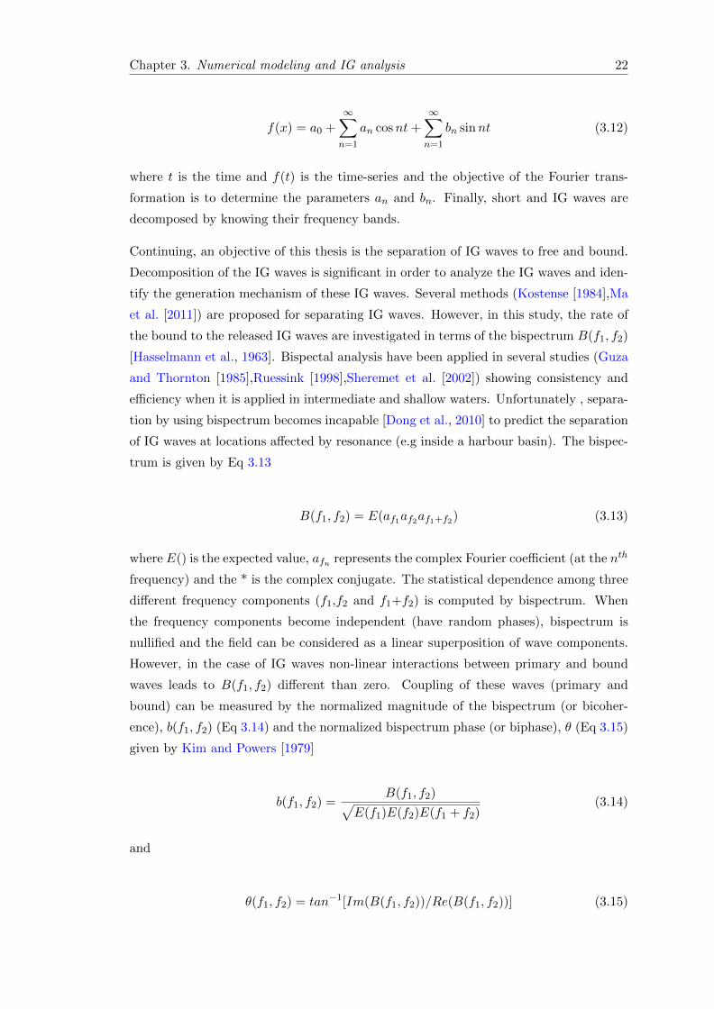
3.2 The spatial variation of the bicoherence over a beach for three wave con-ditions [Eldeberky, 1996]. . . . . . . . . . . . . . . . . . . . . . . . . . . . 23
viii
List of Figures ix
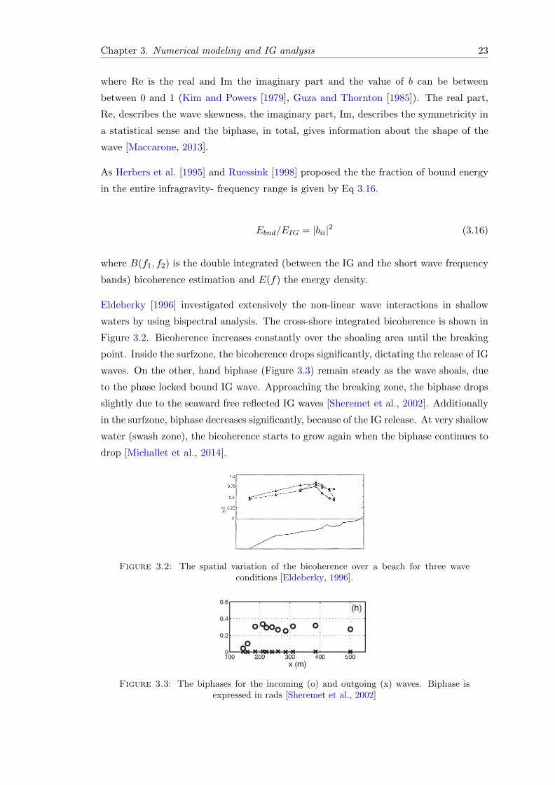
3.3 The biphases for the incoming (o) and outgoing (x) waves. Biphase isexpressed in rads [Sheremet et al., 2002] . . . . . . . . . . . . . . . . . . . 23
3.4 Measured (black triangles), and simulated Hrms,IG and across fringingreef profile . Model results for untuned (left column) and tuned (rightcolumn) breaking parameters are shown for SWASH (solid blue curve),SWAN (dotted red curve), and XBeach (dashed magenta curve) [Buckleyet al., 2014] . . . . . . . . . . . . . . . . . . . . . . . . . . . . . . . . . . . 25
3.5 The reef elevation profile is shown in the bottom row for reference [Buckleyet al., 2014] . . . . . . . . . . . . . . . . . . . . . . . . . . . . . . . . . . . 25
4.1 The location of Barbers Point harbour. . . . . . . . . . . . . . . . . . . . . 27
4.2 A plan view and the bathymetry of Barbers Point harbour. . . . . . . . . 28
4.3 Location of different type of buoys, installed by CDIP around the BarbersPoint harbour. . . . . . . . . . . . . . . . . . . . . . . . . . . . . . . . . . 29
4.4 Offshore boundary energy condition (buoy 159) during the storm of 16-11-1989, 19:30-20:45. Sample length is 3900 seconds,sample rate 1 Hz andthe mean direction is 260 degrees. . . . . . . . . . . . . . . . . . . . . . . . 30
4.5 Offshore boundary energy condition (buoy 159) during the storm of 16-11-1989, 19:30-20:45. Sample length is 4800 seconds, sample rate 1 Hzand the mean direction is 275 degrees. . . . . . . . . . . . . . . . . . . . . 30
4.6 Cross-correlation coefficient between short wave envelope and IG wavesurface elevation ζIG for the storm incident S16. . . . . . . . . . . . . . . 32
4.7 The directional spectrum at the offshore boundary which implemented inSWASH in order to simulate the storm incident S16. . . . . . . . . . . . . 33
4.8 The directional spectrum at the offshore boundary which implemented inSWASH in order to simulate the storm incident S17. . . . . . . . . . . . . 33
4.9 The sponge layers (areas covered by brown color) implemented in thesimulated domain. . . . . . . . . . . . . . . . . . . . . . . . . . . . . . . . 34
5.1 The IG wave energy spectrum for different values of directional spreadingat the location 059-P1. Blue is the measured form CDIP, green forms=10,red for ms=15, cyan for ms=20, magenta for ms=25 and yellow for ms=40. 38
5.2 The IG wave energy spectrum for different values of sponge layer width, atthe location 059-P1. Blue is the measured form CDIP, green for spon=0m, red for spon=100 m, cyan for spon= 200 m and magenta for spon=400 m . . . . . . . . . . . . . . . . . . . . . . . . . . . . . . . . . . . . . . 39
5.3 The IG wave energy spectrum for different values of grid size resolution,at the location 059-P1. Blue is the measured from CDIP, green for 1vertical layer and red for 2 vertical layers. . . . . . . . . . . . . . . . . . . 40
5.4 The IG wave energy spectrum for different number of vertical layers, atthe location 059-P1. Blue is the measured form CDIP, green for 1 verticallayer and red for 2 vertical layers. . . . . . . . . . . . . . . . . . . . . . . . 41
5.5 The IG wave energy spectrum for different dissipation coefficient, at thelocation 059-P1. Blue is the measured form CDIP, green for α = 0.4 andred for α = 0.6 . . . . . . . . . . . . . . . . . . . . . . . . . . . . . . . . . 42
5.6 Energy spectrums calculated at different locations, 066-P1,066-P2,066-P3and 060-P2 compared with the measured spectrums by CDIP. . . . . . . 44
List of Figures x
5.7 The significant IG wave height inside the basin as it is calculated byusing SWASH. The circles represent the measured locations and insidethe circles the value of the IG significant height is the measured one. . . . 44
6.1 Location of the simulated transects, PBr (blue ) and PIn (green). Arrowsshow the mean direction of the waves (total wave signal) for the S16 wavecondition. . . . . . . . . . . . . . . . . . . . . . . . . . . . . . . . . . . . 47
6.2 The bottom profiles, PBr (upper panel) and PIn (bottom panel). Withred color is the bottom profile and with blue the mean water level. . . . 48
6.3 The spectral evolution, in terms of variance energy density (m2/Hz). Theupper panel dictates the energy distribution for the IG waves, (0.005 −0.05Hz), and the bottom panel the energy distribution for the shortwaves,(0.05− 0.25Hz). Both of the panels are showing the energy evolu-tion for the profile PBr . . . . . . . . . . . . . . . . . . . . . . . . . . . . 50
6.4 The spectral evolution, in terms of variance energy density (m2/Hz). Theupper panel dictates the energy distribution for the IG waves, (0.005 −0.05Hz), and the bottom panel the energy distribution for the shortwaves,(0.05− 0.25Hz). Both of the panels are showing the energy evolu-tion for the profile PIn . . . . . . . . . . . . . . . . . . . . . . . . . . . . 51
6.5 The significant height for the IG (red color) and short waves (blue color).Upper panel is the PBr profile and the bottom panel the PIn profile. . . 51
6.6 Examples of the normalized bispectrum for different locations, for thePBr profile. . . . . . . . . . . . . . . . . . . . . . . . . . . . . . . . . . . 52
6.7 Bicoherence, b, for the PBr profile (upper panel) and the PIn profile(bottom panel). . . . . . . . . . . . . . . . . . . . . . . . . . . . . . . . . 54
6.8 The simulated biphase, θ for the PBr profile (upper panel) and the PInprofile (bottom panel). . . . . . . . . . . . . . . . . . . . . . . . . . . . . 54
6.9 The significant height, Hsig, for the bounded IG (red color) and free IGwaves (blue color). Upper panel is the PBr profile and the bottom panelthe PIn profile. . . . . . . . . . . . . . . . . . . . . . . . . . . . . . . . . 55
6.10 Left panels: Bulk fluxes, F, for the incoming (blue) and outgoing (red) IGwaves. Right panels: Reflection coefficient, R2 for the IG band. Upperpanels are related to the PBr profile and bottom panels related to thePIn profile. . . . . . . . . . . . . . . . . . . . . . . . . . . . . . . . . . . 56
B.1 The IG wave energy spectrum for S17 and for different values of direc-tional spreading at the location 059-P1. Blue is the measured form CDIP,green for ms=10, red for ms=15, cyan for ms=20, magenta for ms=25and yellow for ms=40. . . . . . . . . . . . . . . . . . . . . . . . . . . . . . 66
B.2 Energy spectrums calculated for S17 at different locations, 066-P1,066-P2,066-P3 and 060-P2 compared with the measured spectrums by CDIP.. . . . . . . . . . . . . . . . . . . . . . . . . . . . . . . . . . . . . . . . . . 67
C.1 Amplification factor for different locations inside the basin (066-P1,066-P2,066-P3 and 060-P2) for the S16. . . . . . . . . . . . . . . . . . . . . . 69
C.2 Amplification factor for different locations inside the basin (066-P1,066-P2,066-P3 and 060-P2) for the S17. . . . . . . . . . . . . . . . . . . . . . . 70
D.1 The breaking zones (black) for the simulated wave condition S16 accordingto the SWASH bore concept. . . . . . . . . . . . . . . . . . . . . . . . . . 71

List of Figures xi
D.2 The breaking zones (black) for the simulated wave condition S16 accordingto the Weggel [1972] breaking criterion. . . . . . . . . . . . . . . . . . . . 72
E.1 Directional spectrum for the short waves at the location, x = 200m (Pro-file PBr). . . . . . . . . . . . . . . . . . . . . . . . . . . . . . . . . . . . . 73
E.2 Directional spectrum for the IG waves at the location, x = 200m (ProfilePBr). . . . . . . . . . . . . . . . . . . . . . . . . . . . . . . . . . . . . . . 74
E.3 Directional spectrum for the short waves at the location, x = 500m (Pro-file PBr). . . . . . . . . . . . . . . . . . . . . . . . . . . . . . . . . . . . . 74
E.4 Directional spectrum for the IG waves at the location, x = 500m (ProfilePBr). . . . . . . . . . . . . . . . . . . . . . . . . . . . . . . . . . . . . . . 75
E.5 Directional spectrum for the short waves at the location, x = 1200m(Profile PBr). . . . . . . . . . . . . . . . . . . . . . . . . . . . . . . . . . 75
E.6 Directional spectrum for the IG waves at the location, x = 1200m (ProfilePBr). . . . . . . . . . . . . . . . . . . . . . . . . . . . . . . . . . . . . . . 76
E.7 Directional spectrum for the short waves at the location, x = 1460m(Profile PBr). . . . . . . . . . . . . . . . . . . . . . . . . . . . . . . . . . 76
E.8 Directional spectrum for the IG waves at the location, x = 1460m (ProfilePBr). . . . . . . . . . . . . . . . . . . . . . . . . . . . . . . . . . . . . . . 77
E.9 Directional spectrum for the short waves at the location, x = 200m (Pro-file PIn). . . . . . . . . . . . . . . . . . . . . . . . . . . . . . . . . . . . . 77
E.10 Directional spectrum for the IG waves at the location, x = 200m (ProfilePIn). . . . . . . . . . . . . . . . . . . . . . . . . . . . . . . . . . . . . . . 78
E.11 Directional spectrum for the short waves at the location, x = 500m (Pro-file PIn). . . . . . . . . . . . . . . . . . . . . . . . . . . . . . . . . . . . . 78
E.12 Directional spectrum for the IG waves at the location, x = 500m (ProfilePIn). . . . . . . . . . . . . . . . . . . . . . . . . . . . . . . . . . . . . . . 79
E.13 Directional spectrum for the short waves at the location, x = 1200m(Profile PIn). . . . . . . . . . . . . . . . . . . . . . . . . . . . . . . . . . . 79
E.14 Directional spectrum for the IG waves at the location, x = 1200m (ProfilePIn). . . . . . . . . . . . . . . . . . . . . . . . . . . . . . . . . . . . . . . 80
E.15 Directional spectrum for the short waves at the location, x = 1460m(Profile PIn). . . . . . . . . . . . . . . . . . . . . . . . . . . . . . . . . . . 80
E.16 Directional spectrum for the IG waves at the location, x = 1460m (ProfilePIn). . . . . . . . . . . . . . . . . . . . . . . . . . . . . . . . . . . . . . . 81
F.1 Normalized bispectrum (bicoherence) at the location x = 200m for thePIn profile. . . . . . . . . . . . . . . . . . . . . . . . . . . . . . . . . . . . 82
F.2 Normalized bispectrum (bicoherence) at the location x = 500m for thePIn profile. . . . . . . . . . . . . . . . . . . . . . . . . . . . . . . . . . . . 83
F.3 Normalized bispectrum (bicoherence) at the location x = 1200m for thePIn profile. . . . . . . . . . . . . . . . . . . . . . . . . . . . . . . . . . . . 83
F.4 Normalized bispectrum (bicoherence) at the location x = 1460m for thePIn profile. . . . . . . . . . . . . . . . . . . . . . . . . . . . . . . . . . . . 84
List of Tables
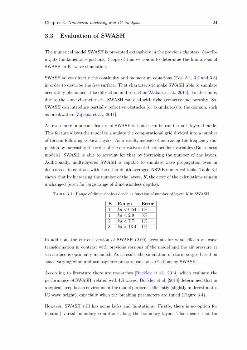
3.1 Range of dimensionless depth as function of number of layers K in SWASH 24
3.2 Advantages and drawbacks of SWASH . . . . . . . . . . . . . . . . . . . . 26
4.1 The duration and the date of the storm incidens . . . . . . . . . . . . . . 29
4.2 Wind speed during the investigated storms . . . . . . . . . . . . . . . . . 31
5.1 Non-given parameters. With V are marked the parameters which areincluded to the sensitivity analysis an with X the parameters which areneglected . . . . . . . . . . . . . . . . . . . . . . . . . . . . . . . . . . . . 37
5.2 The IG wave significant height for different directional spreading valuescompared to the observed one. . . . . . . . . . . . . . . . . . . . . . . . . 38
5.3 The IG wave significant height for different sponge layer widths comparedto the observed one. . . . . . . . . . . . . . . . . . . . . . . . . . . . . . . 40
5.4 The IG wave significant height for different grid sizes compared to theobserved one. . . . . . . . . . . . . . . . . . . . . . . . . . . . . . . . . . . 41
5.5 The IG wave significant height for different grid sizes compared to theobserved one. . . . . . . . . . . . . . . . . . . . . . . . . . . . . . . . . . . 41
5.6 The IG wave significant height for different grid sizes compared to theobserved one. . . . . . . . . . . . . . . . . . . . . . . . . . . . . . . . . . . 42
5.7 The input parameters as defined apriori and tested in the sensitivity analysis 43
6.1 Separation of the profiles PBr and PIn to discrete zones . . . . . . . . . 48
B.1 The IG wave significant height for different directional spreading valuescompared to the observed one (S17 and buoy 059-P1). . . . . . . . . . . . 67
B.2 The IG wave significant height for different locations inside the basincompared with the measured ones (S17). . . . . . . . . . . . . . . . . . . . 67
xii

Abbreviations
IG InfraGravity
SWASH Simulating WAaves till SHore
XBeach eXtream Beach behaviour
FFT Fast Fourier Transformation
RANS Reynolds Averaged Navier Stoke equations
NSWE Non-linear Shallow Water Equations
CDIP Coastal Data Information Program
xiii

To my parents, Ourania and Konstantinos, for their endless love,support and encouragement. . .
xiv
Chapter 1
Introduction
1.1 Background
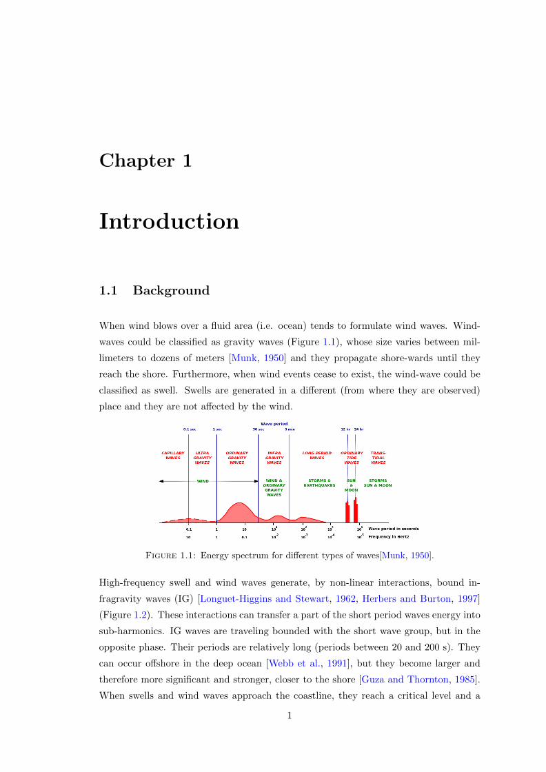
When wind blows over a fluid area (i.e. ocean) tends to formulate wind waves. Wind-
waves could be classified as gravity waves (Figure 1.1), whose size varies between mil-
limeters to dozens of meters [Munk, 1950] and they propagate shore-wards until they
reach the shore. Furthermore, when wind events cease to exist, the wind-wave could be
classified as swell. Swells are generated in a different (from where they are observed)
place and they are not affected by the wind.
Figure 1.1: Energy spectrum for different types of waves[Munk, 1950].
High-frequency swell and wind waves generate, by non-linear interactions, bound in-
fragravity waves (IG) [Longuet-Higgins and Stewart, 1962, Herbers and Burton, 1997]
(Figure 1.2). These interactions can transfer a part of the short period waves energy into
sub-harmonics. IG waves are traveling bounded with the short wave group, but in the
opposite phase. Their periods are relatively long (periods between 20 and 200 s). They
can occur offshore in the deep ocean [Webb et al., 1991], but they become larger and
therefore more significant and stronger, closer to the shore [Guza and Thornton, 1985].
When swells and wind waves approach the coastline, they reach a critical level and a
1
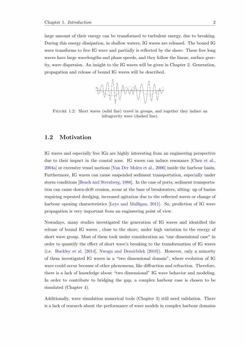
Chapter 1. Introduction 2
large amount of their energy can be transformed to turbulent energy, due to breaking.
During this energy dissipation, in shallow waters, IG waves are released. The bound IG
wave transforms to free IG wave and partially is reflected by the shore. These free long
waves have large wavelengths and phase speeds, and they follow the linear, surface grav-
ity, wave dispersion. An insight to the IG waves will be given in Chapter 2. Generation,
propagation and release of bound IG waves will be described.
Figure 1.2: Short waves (solid line) travel in groups, and together they induce aninfragravity wave (dashed line).
1.2 Motivation
IG waves and especially free IGs are highly interesting from an engineering perspective
due to their impact in the coastal zone. IG waves can induce resonance [Chen et al.,
2004a] or excessive vessel motions [Van Der Molen et al., 2006] inside the harbour basin.
Furthermore, IG waves can cause suspended sediment transportation, especially under
storm conditions [Beach and Sternberg, 1988]. In the case of ports, sediment transporta-
tion can cause down-drift erosion, scour at the base of breakwaters, silting- up of basins
requiring repeated dredging, increased agitation due to the reflected waves or change of
harbour opening characteristics [Leys and Mulligan, 2011]. So, prediction of IG wave
propagation is very important from an engineering point of view.
Nowadays, many studies investigated the generation of IG waves and identified the
release of bound IG waves , close to the shore, under high variation to the energy of
short wave group. Most of them took under consideration an “one dimensional case” in
order to quantify the effect of short wave’s breaking to the transformation of IG waves
(i.e. Buckley et al. [2014], Nwogu and Demirbilek [2010]). However, only a minority
of them investigated IG waves in a “two dimensional domain”, where evolution of IG
wave could occur because of other phenomena, like diffraction and refraction. Therefore,
there is a lack of knowledge about “two dimensional” IG wave behavior and modeling.
In order to contribute to bridging the gap, a complex harbour case is chosen to be
simulated (Chapter 4).
Additionally, wave simulation numerical tools (Chapter 3) still need validation. There
is a lack of research about the performance of wave models in complex harbour domains

Chapter 1. Introduction 3
and their accuracy to predict the transformation and propagation of IG waves due to
refraction, diffraction and partial reflection.
From a scientific point of view, the above mentioned uncertainties, were the reason that
motivated me to proceed to that research.
1.3 Research question
Due to the complexity of the processes taking place in the progression of IG waves in the
offshore but mostly in the near-shore area, there are still uncertainties in the propagation
and transformation of bound IG waves and in the behavior of free IG waves. Numerical
models tend to give inaccurate simulations of IG wave’s evolution, mostly on the shore or
shelf area. More specifically, some of the wave numerical models (i.e. SWASH Zijlema
et al. [2011]) tend to underestimate shoreline reflection and as a result under-predict
the magnitude of free IG waves throughout the domain [Buckley et al., 2014] whereas
other models (i.e. XBeach [Roelvink et al., 2009]) underestimate dissipation and over-
predict the height of IG wave, especially over steep slopes [Buckley et al., 2014]. The
number of these uncertainties are increasing when the domain of investigation becomes
two dimensional because of complex phenomena like diffraction, refraction, reflection
and the existence of edge waves (Chapter 2.3).
Scope of this study is to provide insight in the propagation of bound IG waves and
focus on the generation and evolution of free IG waves by using a wave numerical tool
for near-shore areas. Emphasis will be given on their simulation and their effects in
harbours. Leading to the primary research question in this thesis project:
“Which are the generation mechanisms of infragravity waves, how do they propagate
through the domain and how the processes can be modeled in a two-dimensional case ?”
1.4 Objectives
The main objective of this thesis is to obtain insight in the generation, evolution, energy
dissipation and separation of IG waves in two categories, the bound and the free part.
Furthermore, this knowledge will be used to simulate IG wave propagation and effects,
in a harbour case.
To answer the research question and fulfill the major objective a number of secondary
questions are formulated:
Chapter 1. Introduction 4
1. For Chapter 2, Infragravity waves
(a) How are bound IG waves generated and under which typical conditions?
(b) How are free IG waves generated, how could they be classified according to
their origin and how important is each classification for harbour cases?
(c) Which are the dissipation mechanisms of IG waves?
2. For Chapter 3, Numerical modeling
(a) Which are the most widely used wave numerical models and how they could
be characterized?
(b) According to literature, which are the limitations of the numerical tools in a
two-dimensional IG wave simulation ?
(c) Are these IG wave models capable to directly provide characteristic of IG
waves (i.e. significant height), or is an additional method required for output
analysis?
(d) According to the obtained knowledge, which model(s) has to be used in or-
der to obtain accuracy and reasonable computational time (in Barbers Point
harbour case)?
3. For Chapter 4 and Chapter 5, Barbers Point Harbour (two-dimensional) case
(a) Determine the simulation time in order to achieve statistically accurate cal-
culation for the IG waves
(b) How large and what resolution in space and time should the simulated domain
have, and what will be the effects to the accuracy and duration of simulation?
(c) What boundary conditions are required?
(d) What are the reflection characteristics of boundary (shore) layers?
(e) How sensitive is the numerical wave model for the unknown input parameters
(i.e. grid resolution, breaking parameters,sponge layers) ?
(f) How accurate are the calculations of the IG waves compared to field mea-
surements (model validation)?
4. For Chapter 6, IG wave decomposition
(a) Is bispectral analysis (as a decomposition method) applicable inside the basin?
(b) How can we decompose the incoming from the out-coming IG wave?
(c) How do short waves transmit energy to IG waves and dependable is this
transmission on the depth (intermediate depths, surf-zone) ?
(d) How the IG wave behave when it is reflected (fully or not reflected)?
Chapter 1. Introduction 5
These are the main research question which are addressed in this thesis. A summary of
answers is given in Chapter 7.
1.5 Thesis outline
The initial step in the present study is to identify the fundamental characteristics of IG
waves. Insight in the generation, propagation, dissipation (in the offshore and near-shore
area) and reflection of IG waves is obtained in Chapter 2. Simultaneously, discretization
of different types of IG waves depending on their relevancy to harbour problems is
presented. Then, Chapter 3 presents the available numerical wave models, an extensive
comparison of them, and concludes to that one which performs more accurate in the
case of Barbers Point harbour. Both of these chapters are part of the literature review.
Chapter 4 presents the case which is selected to be investigated. IG wave behavior is
investigated for the case of Barbers Point harbour in Oahu, Hawaii, USA. Additionally,
the bathymetry and the offshore wave conditions are shown. Finally, there is a first
try to identify the correlation of the IG with the short waves, in order to determine,
qualitatively, the boundedness between IG-short waves.
However, there are several parameters (i.e sponge layers) which are not available a
priori and there are important to achieve an accurate simulation. A sensitivity analysis
(Chapter 5) for these parameters is carried out, in order to define them. Finally, the
input data are determined and the simulated IG wave characteristics are compared with
the field measurements (model validation).
Finally, in Chapter 6, IG wave is analyzed by using bispectral analysis. The aim is to
decompose the IG wave to the free and bounded component. The last step is a further
separation of the IG wave to the incoming and outgoing part by using the method of
Sheremet et al. [2002].
Conclusions and recommendations for future research are given in Chapter 7.

Chapter 2
Infragravity waves
As explained in Chapter 1, infragravity waves are surface gravity waves with long periods
(0.005- 0.05 Hz) and their energy contribution is presented in Figure 1.1. Firstly, they
observed as surf-beat and determined by Longuet-Higgins and Stewart [1962]. Due to
non-linear interactions between group of high waves, bounded (to this group) IG waves
are generated and their energy increases shore-wards. After high variabilities (spatial
and temporal) in the energy of the group (i.e. breaking, reflection), they are released in
the form of freely propagating waves. Recent studies have shown that they are important
(high impact) to coastal-zone areas, such as oscillations in harbours, sediment transport
and excessive motions to the moored vessels (Chapter 1.2).
In this section, an extensive presentation of IG wave’s generation and spatial behavior,
and formation differences of free IG waves are given. The study is harbour engineering
oriented and as a result there will be a presentation of significance of each IG wave
formation (bound, free, leaky and edge IG wave) for the design of ports.
2.1 Generation and propagation
In offshore regions wind waves are generated and they tend to travel in groups. It is
observed that the water level is depressed under such a group of waves. This depression
can be explained by using the radiation stress concept of Longuet-Higgins and Stewart
[1962].
According to Longuet-Higgins and Stewart [1962], a group of waves outside the boundary
layers contains a second-order vorticity, which is associated with a steady second-order
current (bound IG wave) and does not affect the distribution of pressure. After the
identification of IG waves, Longuet-Higgins and Stewart [1962] provided a second-order
6

Chapter 2. Infragravity waves 7
solution for the surface elevation ζ and the velocity potential φ by expanding the Stokes
method of approximation:
ζ = ζ(1) + ζ(2) + ... (2.1)
φ = φ(1) + φ(2) + ... (2.2)
where ζ(1) and φ(1) satisfy the linearised equations and boundary conditions and ζ(1)+ζ(2),
φ(1)+φ(2) satisfy the equations as far as the quadratic terms and so on. For simplicity
reasons, if it is assumed that incident wave consists of two unidirectional harmonics
(bichromatic), the solution follows up for Eqs.(2.3 and 2.4).
ζ = ζ1 + ζ2 + ζ1,2 (2.3)
φ = φ1 + φ2 + φ1,2 (2.4)
where ζ1, ζ2, φ1 and φ2 are relevant with the primary short waves and ζ1,2 and φ1,2 are
describing the second-order solution which is a combination of a sub (i.e. bound IG wave)
and a super harmonic wave, which are forced by the difference and sum interactions,
respectively [Rijnsdorp et al., 2012]. Figure 2.1 shows the energy transmission to sub
and super harmonics, as the waves propagate, for a narrow peaked spectrum [Michallet
et al., 2014].
Figure 2.1: Spectral evolution as a friction of the cross-shore position (x) and thefrequency (f) [Michallet et al., 2014]
Bound IG, as predicted from the second-order Stokes theory, is quadratic related to the
energy of shorter energies (Figure 2.2) and that relation confirmed by Herbers et al.
[1995], who investigated this relation in high depths, where bound IG waves are gener-
ated.
Recent studies suggested that the propagation of bound IG waves depends on its fre-
quency [Battjes et al., 2004]. When its frequency is relatively high, IG wave behaves
as Longuet-Higgins and Stewart [1962] described. On the other hand, when frequency
decreases, IG wave can be described more accurately by Green’s law [Synolakis, 1991].
As Battjes et al. [2004] observed this is caused because of the (slightly) larger phase dif-
ferences of the lower frequencies, which allows more energy to be transformed from the

Chapter 2. Infragravity waves 8
Figure 2.2: Bound IG wave energy compared with swell energy for different locations.Energy decreases as depth increases [Herbers et al., 1995].
group of short waves. Cross-shore energy evolution per wave frequency band is shown
in Figure 2.3.
Finally, bound IG waves can cause direct impact to the harbours only during storms and
due to swells [Nakaza and Hino, 1991]. Additionally, negative effects on the construction
depend on the width of the entrance and how much bound IG wave energy will penetrate
to the harbour. In most of the cases, harbours are well protected from short waves and
their bounded long waves but it is hard to prevent the existence of released long waves
(Chapter 2.2), which are propagating freely.
2.2 Incident free long waves
Generally, generation mechanism of free IG can be separated in two categories:

Chapter 2. Infragravity waves 9
Figure 2.3: Hm0 values of incoming (triangles) and outgoing (dots) IG waves fordifferent frequency bands. Lower dashed curve: Green (H ∼ h1/4), fitted to outgoingwave heights in the zone offshore from x = 20 m; upper dashed curve: Longuet-Higginsand Stewart [1962] asymptote (H ∼ h5/2), initiated with wave height at x = 8 m.[Battjes
et al., 2004]
• Bound IG waves generated by non-linear interactions are released as free when
high decrease in the short wave energy is occurred [Longuet-Higgins and Stewart,
1962].
• Time-varying break point of short wave groups [Symonds et al., 1982].
Firstly, Longuet-Higgins and Stewart [1962] investigated the generation of IG waves and
argued that they are propagating bounded with short wave groups. In the surf zone (or
wherever there are high fluctuations to the short wave energy) the wave group dissipates
and the IG wave is released. On the other hand Symonds et al. [1982] suggested that
due to the radiation stress strong gradients in the surf zone, a set up at the shore line
is caused. The conclusion is that the break point varies through time and this set-up
(which varies with the time wave group scale) can be recognized as a free IG wave
propagating shore-wards (in phase) and seawards (out of phase). According to Battjes
et al. [2004] and Dong et al. [2009], the second mechanism is dominant at steep slopes
and the first to the milder.
In contrast with the more quadratic relation of swell/storm and bound IG wave, free IG
waves seem to be more linearly proportional to the short waves (Figure 2.4). Herbers
et al. [1995] determined that breaking is the most important generation procedure for
free IG waves. However, Zhou and Liu [1987] proved theoretically, that bound IG waves
could be released as free due to the diffraction, close to the basin’s inlet. Still, there
is no research (especially on the field) which agrees with that release mechanism. The
investigation of IG release is done by using bispectral analysis and more details about
this method are presented in Chapter 3.2.

Chapter 2. Infragravity waves 10
Figure 2.4: Linear relation of free IG waves measured in different locations [Herberset al., 1995].
Nowadays, modern harbour designers tend to locate the entrance in a water depth (at
least) twice the height of a design storm wave, in order to prevent negative impacts,
on vessels, by wave breaking [McBride et al., 1996]. This channel depth is depending
mainly on draught and wave length. Aim of harbour engineers is to avoid wave breaking
phenomenon inside the channel or in the basin. However, this does not mean that
harbours are protected by free long waves generated by breaking. McComb et al. [2009]
proved that high energies from long waves that can induce resonance originated from
free IG waves. These free IG waves are generated by breaking in the adjacent reef area
and refracted, due to the entrance channel, inside the basin (Figure 2.5).
2.3 Reflected infragravity waves
IG waves are considered fully reflected from the shore or partially by an obstacle (i.e.
wall, breakwater) [Sheremet et al., 2002, Herbers et al., 1995, Battjes et al., 2004]. After
their reflection IG waves can de-shoal to offshore regions (leaky wave) or remain trapped
into the surfzone (edge wave). Decomposition of reflected waves is complex but it can be
done by using the wave number spectrum [Holland and Holman, 1999] and it is presented
Figure 2.6. According to Holland and Holman [1999], in the frequency band of IG waves
(0.005-0.05 Hz), high absolute and low absolute wave numbers represent edge and leaky
waves respectively.

Chapter 2. Infragravity waves 11
Figure 2.5: Upper plot shows the typical swell wave patterns, lower plot details aboutthe topography and the areas where free IG waves refracted and penetrate to the basin
[McComb et al., 2009].
Figure 2.6: A typical separation of reflected IG waves according to their wave-number,presented by Holland and Holman [1999]

Chapter 2. Infragravity waves 12
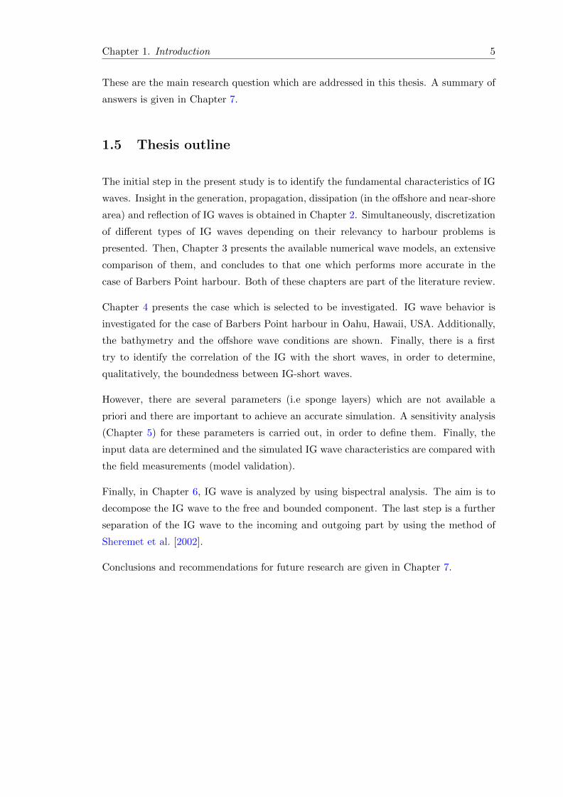
As explained leaky waves are freely seaward propagating IG waves (Figure 2.11, panel
(d), (e) and (f)). They are generated from an obstacle and they are important for
near-shore sediment transport and creation of standing waves close to beaches (surf or
swash zone). From a harbour engineering perspective, leaky waves are important for the
construction because they can induce oscillations to the moored vessels inside the basin
[Harkins and Briggs, 1994].
The lateral type of reflected IG wave is the edge wave (Figure 2.9). When the angle
of the incident wave is relatively high the free IG reflected wave can be trapped due
to refraction in the surf-zone (Figure 2.10). Firstly, edge waves identified by Stokes
who tried to determine their propagation speed. Finally, Ursell [1952] proved that edge
waves can be described by different modes and that the Stokes theory consist the lowest
of these modes. These modes represents the number of zero amplitude crossings, in
cross-shore direction (Figure 2.7).
Figure 2.7: Three different edge wave modes (0,1 and 2) [Van Giffen, 2003]
In order to determine the incoming and outgoing (reflected) IG waves the method of
Sheremet et al. [2002] is proposed. The energy of the incoming and reflected waves are
calculated as:
E±(f) = 0.25(Coηη(f) + h/gCouu(f)± (2√h/g)Coηu(f) (2.5)
and the corresponding IG energy flux is given by:
F±(f) = E±(f)√gh (2.6)
where Coηu is the cospectrum between the surface elevation (η) and the velocity for
the mean direction (u). Furthermore, Coηη and Couu is the autospectra for the surface
elevation and the velocity, respectively, h is the depth and g is the gravitational acceler-
ation. Finally both energies (E) and fluxes (F ) are calculated for the IG wave frequency
band (0.005-0.05 Hz). Reflection coefficient (R) is given by:
Chapter 2. Infragravity waves 13
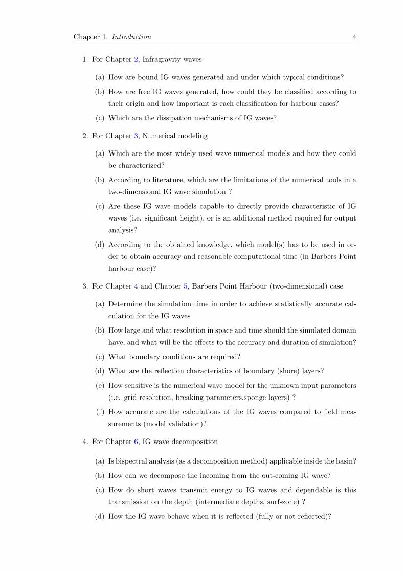
R2 = F−/F+ (2.7)
de Bakker et al. [2013] determined that the incoming fluxes grow until the breaking
point and after that diminishes, when the outgoing flux remains relatively constant
(Figure 2.8, upper panel). The reflection coefficient (Figure 2.8, bottom panel) slightly
decreases close (from the offshore side) to the breaking point and after that becomes
steady.
Figure 2.8: (a) Bulk incoming (circles) and outgoing (black dots) infragravity energyfluxes (F±) and (b) bulk reflection coefficients (R2) for the infragravity wave band
[de Bakker et al., 2013].
From an engineering perspective, existence of edge waves can cause resonance to har-
bours and oscillations to vessels. Negative impact of edge waves proved theoretically
by Bowers [1977] and practically by Ciriano et al. [2001] and Chen et al. [2004b]. The
complex effects of edge waves are under investigation and it is difficult to propose proper
solutions for this new type of resonance. Nowadays, harbour engineers are capable to
counter the lowest (simplest) modes of these edge waves by redirecting the reflected IG
waves. Breakwaters alongshore and inside the surfzone could redirect the edge waves
outside of a harbour basin as Chen et al. [2004b] proposed.
2.4 Dissipation mechanisms
At low water depths and close to the shore, IG waves energy decreasing. This energy
dissipation can be caused by several reasons and in this research the most significant of
them, according to literature, are presented.

Chapter 2. Infragravity waves 14
Figure 2.9: Propagation of a Stokes (zero mode) edge wave alongshore [Van Giffen,2003] .
Figure 2.10: Generation of an edge wave due to de-shoaling and refraction [Van Giffen,2003] .
At first, Thomson et al. [2006] determined that it is possible reflected IG waves transmit
some of their energy to the short wave groups. This can occur inside the surf-zone before
the breaking point. Eventually, this energy will be dissipated after the breaking of short
waves. This mechanism can be interesting when engineers are trying to simulate the
propagation of edge waves.
Additional, an other dissipation mechanism can be the breaking of IG wave as Van Don-
geren et al. [2007] explained. Under extreme storm conditions, freely propagating IG
wave can continue the shoaling process shore-wards and at a certain point, breaks (Fig-
ure 2.11, panel (b)).
The last mechanism is bottom friction. Henderson and Bowen [2002] proved that energy
of IG wave can dissipate due to the bottom friction. However, more recent research by
Henderson et al. [2006] determined that for small drag coefficients this mechanism can
be neglected. Furthermore, Rijnsdorp et al. [2014] showed that the bottom friction has
marginal effect on incoming IG waves. In case of mildly reflective, bottom friction has
a significant influence on the evolution of outgoing IG waves.
Chapter 2. Infragravity waves 15
Figure 2.11: Significant wave height versus cross-shore distance x for (a) short wavesHs and (b) infragravity waves Hinf for different locations: A1 (black dots), A2 (light-grey dots) and A3 (dark-grey dots). (c) Bed profile. Furthermore, the significantincoming (circles) and outgoing (black dots) infragravity-wave heights calculated fromseparated signals (following Guza et al., 1984) are shown for (d) A1, (e) A2 and (f) A3
[de Bakker et al., 2013].

Chapter 3
Numerical modeling and IG
analysis
Recently many numerical models developed in order to simulate wave transformation
and morphological processes. Nowadays, two main classes of wave models are available:
• Phase-averaged models: operate in a frequency domain
• Phase-resolving models: operate in a time domain
Phase-averaged models are not capable to calculate surface elevation in an exact location,
but they predict the average variance (or energy) of surface elevation . Results of a
phase-averaged model correspond to integral spectral wave parameters (i.e. significant
wave height) of the wave field. They are using the energy balance equation in order to
describe the spectral evolution and they considered as ”computational cheap”. Due to
these characteristics, they are suitable for simulating cases over long distances where the
depth changes slowly [Monbaliu et al., 2000]. These models neglect or approximate wave
transformation processes such as wave diffraction, reflection, and non-linear interactions,
so they are not able to simulate accurately IG waves.
Phase-resolving models are able to calculate sea surface in time and space by using one
of these three types of equations:
• Reynolds Averaged Navier Stoke equations (RANS)
• Boussinesq equations
• Non-linear shallow water equations (NSWE)
16

Chapter 3. Numerical modeling and IG analysis 17
• Mild-Slope equations
Output of these models is a picture of sea surface elevation fields for each of the modelling
time step which makes them computationally expensive. In contrast with phase-averaged
models, they can simulate accurately phenomena like diffraction, refraction an reflection
and calculate IG wave characteristics. Phase-resolving models are used in small domains
where there are rapidly changes to the wave local properties (i.e harbours, close to
breakwaters).
Compared to Boussinesq models (i.e. SURF-GN [Bonneton et al., 2011]), implementa-
tion of NSWE models is less complex, thereby they have improved robustness and it is
easier to maintain them [Rijnsdorp et al., 2012]. Additionally, Boussinesq models are
able to calculate both short and long waves, including all the relevant processes (i.e.
refraction, diffraction, non-linearity) and the bulk dissipation associated with the wave
breaking, but not the detailed breaking process itself [Rijnsdorp et al., 2014]. Neverthe-
less, Boussinesq models applied and validated for short wave motions, including breaking
(i.e. Tonelli and Petti [2012], Tissier et al. [2012]), but only a minority of them extended
to IG wave investigation [Madsen et al., 1997]. On the other hand, NSWE models have
shown great potential to simulate wave propagation, including non-linear wave-dynamics
[Rijnsdorp et al., 2014, Smit et al., 2013] and to calculate accurately IG-motions [Rijns-
dorp et al., 2012, Ma et al., 2012]. Finally, NSWE can perform accurately and with the
same computational effort as Boussinesq models. Finally, Boussinesq models are not
accurate in deeper water due to the absence of vertical-layer discretization [Rijnsdorp
et al., 2014].
Furthermore, RANS models (i.e COBRAS-UC [Lara et al., 2008]) need a lot of computa-
tional resources [Suzuki et al., 2012] especially when the case is two-dimensional. RANS
models can not efficiently compute the free surface flow by considering the free surface as
a single valued function (as NSWE models are able to do) and due to this characteristic
are relatively computational ”expensive” [Rijnsdorp et al., 2014]. Mild-slope models are
limited and they can not take into account the phenomenon of reflection [Lee et al.,
1998]. This feature of the mild-slope models make them unsuitable for harbour cases
and steep-slopes.
NSWE models are relatively (computationally) cheap and applicable for harbour cases
and steep slopes in intermediate and shallow depths. Additionally, the implementation
of the non-hydrostatic term makes them capable to take into account weakly disper-
sive waves (i.e. IG waves). The most widely used non-hydrostatic NSWE models are
the SWASH [Zijlema et al., 2011] and XBeach- non-hydrostatic Roelvink et al. [2009].
XBeach- non-hydrostatic and SWASH is based upon Stelling and Zijlema [2003].

Chapter 3. Numerical modeling and IG analysis 18
In XBeach, vertically a compact scheme is used which allows an inclusion of the boundary
condition of the dynamic pressure at the free surface. The dispersive waves can be
modeled using a depth average flow model. The application of momentum conservative
numerical schemes allows the accurate modelling of wave breaking without the need of
a separate breaking model. However, because XBeach is a depth averaged model, only
the single layer version was implemented. Due to the one-layer feature XBeach (like
Boussinesq models) is inaccurate at large depths. A comparison of XBeach with SWASH
is given in Figure 3.4,showing that XBeach tends to underestimate and overestimate IG
waves at the breaking and surf-zone respectively, due to the low vertical resolution.
In this thesis, the open-source and widely used numerical model SWASH [Zijlema et al.,
2011] is used in order to simulate accurately IG wave propagation and transformation
(Chapter 3). SWASH is a phase-resolving NSWE model and it can run in a multi-layered
mode with improved frequency dispersion properties. SWASH is considered capable to
simulate IG waves [Buckley et al., 2014] and its fundamental characteristics will be
presented in Chapter 3.1. Aim is to conclude to the advantages and the limitations of
SWASH for a two-dimensional case .
3.1 SWASH
SWASH (Simulating WAves till SHore) is a non-hydrostatic, phase-resolving non-linear
wave numerical model, developed by Zijlema et al. [2011]. It is a general-purpose
numerical-tool for simulating hydrodynamic and transport phenomena in shallow water
areas. Furthermore, simulations could be two or even three dimensional. Aim of this
model is to provide an efficient and robust model which can applied in complex domains
like harbours, rivers, estuaries and large-scale oceans.
3.1.1 Fundamental equations
Objective of this section is to present and give insight to SWASH governing equations.
It should be mentioned that SWASH is capable to discretize the domain in vertical
direction and simulate that as equidistant layers. In order to describe the free-surface,
model solves the NSWE including the term of non-hydrostatic pressure (derived by
Navier-Stokes equations) for an incompressible flow.
∂ζ
∂t+∂hu
∂x+∂hv
∂y= 0 (3.1)
∂u
∂t+ u
∂u
∂x+ v
∂u
∂y+ g
∂ζ
∂x+
1
h
∫ ζ
−d
∂q
∂xdz + cf
u√u2 + v2
h=
1
h(∂hτxx∂x
+∂hτxy∂y
) (3.2)

Chapter 3. Numerical modeling and IG analysis 19
∂v
∂t+ u
∂v
∂x+ v
∂v
∂y+ g
∂ζ
∂x+
1
h
∫ ζ
−d
∂q
∂xdz + cf
v√u2 + v2
h=
1
h(∂hτyx∂x
+∂hτyy∂y
) (3.3)
where x and y is the cartesian coordinates, t is the time, ζ is the surface elevation from
the still water level, d is the still water depth, h=ζ+d is the total water depth, u and
v the depth-averaged flow velocities, q the non-hydrostatic pressure, g the gravitational
acceleration, cf the bottom friction coefficient and τxx, τxy,τyx and τyy are the turbulent
stress terms.
According to Stelling and Zijlema [2003] non-hydrostatic pressure q can be expressed
as: ∫ ζ
−d
∂q
∂xdz =
1
2h∂qb∂x
+1
2qb∂(ζ − d)
∂x(3.4)
where qb is the non-hydrostatic pressure at the bottom. Combination of Keller-box
method [Lam and Simpson, 1976] and momentum equations for the vertical velocities
in z-direction at the free surface, ws, and at the bed level, wb, produce Eq 3.5 .
∂ws∂t
=2qbh− ∂wb
∂t(3.5)
Additionally, vertical velocity wb, can be given from the kinematic condition:
wb = −u∂d∂x− v∂d
∂y(3.6)
At the end, velocities can be expressed from the conservation of local mass as:
∂u
∂x+∂v
∂y+ws − wb
h= 0 (3.7)
To conclude, SWASH model tends to solve the tree Eqs. 3.1, 3.2 and 3.3 in order to
determine the values of three unknowns, flow velocities u and v and the surface elevation
ζ, at each layer.
3.1.2 Boundary conditions
A simplified version of the domain is presented to the Figure 3.1 which shows the bound-
aries. Conditions, which are used in order to solve Eqs. 3.1, 3.2 and 3.3, are given for
each boundary, separately. In general, boundary conditions for SWASH are layer av-
eraged velocities and surface elevation series. These series can be imposed directly or
estimated by the model from spectra or fourier parameters.
Chapter 3. Numerical modeling and IG analysis 20
Figure 3.1: Simplification of the domain with the different types of the boundaries.
3.1.2.1 Offshore
An incident wave(s) can be imposed as uni or multi-directional. For regular waves,
the parameters of height and period have to be specified. Alternatively, a surface time
series can be implemented. On the other hand, when the waves are irregular user has to
choose between the spectrum or a time series as input data. Shapes of spectrum can be
either the usual (Jonswap, Pierson-Moskowitz), TMA (modified from the user) or given
entirely form the user (1-D non-directional or 2D directional wave spectrum).
Additionally, a weakly reflective condition which allows outgoing waves and avoid the
reflection of incoming is introduced [Blayo and Debreu, 2005]:
ub = ±√g
h(2ζb − ζ) (3.8)
3.1.2.2 Shore
Generally, shore is assumed a moving shoreline in order to take into consideration wave
run-up and inundations. In addition, obstacles like constructions and breakwaters are
schematized by including their slopes and by means of porosity layers (rubble mound
breakwaters). Constructions are highly reflectional and because of that the Sommerfeld’s
radiation condition (Eq. 3.9) is implemented, which allows reflective waves to cross the
offshore boundary layer.∂u
∂t+√gh∂u
∂x= 0 (3.9)

Chapter 3. Numerical modeling and IG analysis 21
3.1.2.3 Lateral boundary
A lateral boundary is implemented in order to be viable the calculation of Eqs. 3.1, 3.2
and 3.3 in the Open-Lateral (along-shore) boundary (Figure 3.1) direction. For sim-
plicity, it is better to assume that as fully reflective. These assumption yields to locate
gauges (location of interest) outside of the effected area from ”lateral boundary”reflected
waves.
3.1.3 Wave breaking
In Chapter 1 and in Chapter 2, it is identified that breaking phenomena have a major
contribution to the IG wave release. The wave breaking structure is defined by using
SWASH and the bore formation concept [Smit et al., 2013]. The initiation of a wave
breaking process occurs when the fraction of the shallow water celerity is lower than the
vertical speed of the free surface (Eq 3.10).
dζ
dt> a
√gh (3.10)
where a is a parameter related to the surface slope and ζ is the surface elevation. By
default, a is 0.6, which corresponds to the front steepness of 25o. The wave breaking
zone continues until the local steepness reach the value β (by default 0.15) (Eq 3.11).
dζ
dt< β
√gh (3.11)
3.2 Post data analysis and the decomposition of IG waves
The fist step of the post data analysis is the separation of short and IG waves. In order
to achieve that a wave energy spectrum has to be constructed for each simulated location
point. Energy spectrum visualize the magnitude of all the possible wave frequencies. In
order to construct the wave energy spectrum FFT (Fast Fourier Transform) is considered
as the most valuable, signal analysis, computational tool.
Aim of the FFT method is to efficiently compute the Fourier transform. For given time-
series, Fourier transform decomposes the signal to the frequencies that it is considered.
Result is infinite sine and cosine waves with frequencies that start form 0 and increase
in integer multiples of a base frequency (1 divided by total length of the time signal).
Fourier series are given by Eq 3.12
Chapter 3. Numerical modeling and IG analysis 22
f(x) = a0 +
∞∑n=1
an cosnt+
∞∑n=1
bn sinnt (3.12)
where t is the time and f(t) is the time-series and the objective of the Fourier trans-
formation is to determine the parameters an and bn. Finally, short and IG waves are
decomposed by knowing their frequency bands.
Continuing, an objective of this thesis is the separation of IG waves to free and bound.
Decomposition of the IG waves is significant in order to analyze the IG waves and iden-
tify the generation mechanism of these IG waves. Several methods (Kostense [1984],Ma
et al. [2011]) are proposed for separating IG waves. However, in this study, the rate of
the bound to the released IG waves are investigated in terms of the bispectrum B(f1, f2)
[Hasselmann et al., 1963]. Bispectal analysis have been applied in several studies (Guza
and Thornton [1985],Ruessink [1998],Sheremet et al. [2002]) showing consistency and
efficiency when it is applied in intermediate and shallow waters. Unfortunately , separa-
tion by using bispectrum becomes incapable [Dong et al., 2010] to predict the separation
of IG waves at locations affected by resonance (e.g inside a harbour basin). The bispec-
trum is given by Eq 3.13
B(f1, f2) = E(af1af2af1+f2) (3.13)
where E() is the expected value, afn represents the complex Fourier coefficient (at the nth
frequency) and the * is the complex conjugate. The statistical dependence among three
different frequency components (f1,f2 and f1+f2) is computed by bispectrum. When
the frequency components become independent (have random phases), bispectrum is
nullified and the field can be considered as a linear superposition of wave components.
However, in the case of IG waves non-linear interactions between primary and bound
waves leads to B(f1, f2) different than zero. Coupling of these waves (primary and
bound) can be measured by the normalized magnitude of the bispectrum (or bicoher-
ence), b(f1, f2) (Eq 3.14) and the normalized bispectrum phase (or biphase), θ (Eq 3.15)
given by Kim and Powers [1979]
b(f1, f2) =B(f1, f2)√
E(f1)E(f2)E(f1 + f2)(3.14)
and
θ(f1, f2) = tan−1[Im(B(f1, f2))/Re(B(f1, f2))] (3.15)
Chapter 3. Numerical modeling and IG analysis 23
where Re is the real and Im the imaginary part and the value of b can be between
between 0 and 1 (Kim and Powers [1979], Guza and Thornton [1985]). The real part,
Re, describes the wave skewness, the imaginary part, Im, describes the symmetricity in
a statistical sense and the biphase, in total, gives information about the shape of the
wave [Maccarone, 2013].
As Herbers et al. [1995] and Ruessink [1998] proposed the the fraction of bound energy
in the entire infragravity- frequency range is given by Eq 3.16.
Ebnd/EIG = |bii|2 (3.16)
where B(f1, f2) is the double integrated (between the IG and the short wave frequency
bands) bicoherence estimation and E(f) the energy density.
Eldeberky [1996] investigated extensively the non-linear wave interactions in shallow
waters by using bispectral analysis. The cross-shore integrated bicoherence is shown in
Figure 3.2. Bicoherence increases constantly over the shoaling area until the breaking
point. Inside the surfzone, the bicoherence drops significantly, dictating the release of IG
waves. On the other, hand biphase (Figure 3.3) remain steady as the wave shoals, due
to the phase locked bound IG wave. Approaching the breaking zone, the biphase drops
slightly due to the seaward free reflected IG waves [Sheremet et al., 2002]. Additionally
in the surfzone, biphase decreases significantly, because of the IG release. At very shallow
water (swash zone), the bicoherence starts to grow again when the biphase continues to
drop [Michallet et al., 2014].
Figure 3.2: The spatial variation of the bicoherence over a beach for three waveconditions [Eldeberky, 1996].
Figure 3.3: The biphases for the incoming (o) and outgoing (x) waves. Biphase isexpressed in rads [Sheremet et al., 2002]
Chapter 3. Numerical modeling and IG analysis 24
3.3 Evaluation of SWASH
The numerical model SWASH is presented extensively in the previous chapters, describ-
ing its fundamental equations. Scope of this section is to determine the limitations of
SWASH in IG wave simulation.
SWASH solves directly the continuity and momentum equations (Eqs. 3.1, 3.2 and 3.3)
in order to describe the free surface. That characteristic make SWASH able to simulate
accurately phenomena like diffraction and refraction[Alabart et al., 2014]. Furthermore,
due to the same characteristic, SWASH can deal with dyke geometry and porosity. So,
SWASH can introduce partially reflective obstacles (or boundaries) to the domain, such
as breakwaters [Zijlema et al., 2011].
An even more important feature of SWASH is that it can be run in multi-layered mode.
This feature allows the model to simulate the computational grid divided into a number
of terrain-following vertical layers. As a result, instead of increasing the frequency dis-
persion by increasing the order of the derivatives of the dependent variables (Boussinesq
models), SWASH is able to account for that by increasing the number of the layers.
Additionally, multi-layered SWASH is capable to simulate wave propagation even in
deep areas, in contrast with the other depth averaged NSWE numerical tools. Table 3.1
shows that by increasing the number of the layers, K, the error of the calculations remain
unchanged (even for large range of dimensionless depths).
Table 3.1: Range of dimensionless depth as function of number of layers K in SWASH
K Range Error
1 kd < 0.54 1%
1 kd < 2.9 3%
2 kd < 7.7 1%
3 kd < 16.4 1%
In addition, the current version of SWASH (2.00) accounts for wind effects on wave
transformation in contrast with previous versions of the model and the air pressure at
sea surface is optionally included. As a result, the simulation of storm surges based on
space varying wind and atmospheric pressure can be carried out by SWASH.
According to literature there are researches [Buckley et al., 2014] which evaluate the
performance of SWASH, related with IG waves. Buckley et al. [2014] determined that in
a typical steep beach environment the model performs efficiently (slightly underestimates
IG wave height), especially when the breaking parameters are tuned (Figure 3.4).
However, SWASH still has some lacks and limitations. Firstly, there is no option for
(spatial) varied boundary conditions along the boundary layer. This means that (in

Chapter 3. Numerical modeling and IG analysis 25
Figure 3.4: Measured (black triangles), and simulated Hrms,IG and across fringingreef profile . Model results for untuned (left column) and tuned (right column) breakingparameters are shown for SWASH (solid blue curve), SWAN (dotted red curve), and
XBeach (dashed magenta curve) [Buckley et al., 2014] .
Figure 3.5: The reef elevation profile is shown in the bottom row for reference [Buckleyet al., 2014] .
the boundary) although the water depth is different, the input wave conditions have
to be stable (same characteristics) along to the boundary. This limitation can produce
inaccuracies when the waves are not perpendicular to the boundary and the slope of the
bottom is steep.
An additional drawback of SWASH is the way it models breakwaters. SWASH accounts
for the characteristics of the breakwater, like the porosity, as the same for each verti-
cal layer in the same spot of the domain. This assumption of SWASH leads to errors,
especially when mound breakwaters are implemented. In addition the Forchheimer dissi-
pative terms [Verruijt et al., 1970] are not included in the vertical momentum equations,
as Mellink [2012] suggested.
Inaccuracies close to the shore could be caused by the high sensitivity of SWASH to the
bottom friction variations, for the cases of mildly reflective IG wave conditions [Rijnsdorp
et al., 2014]. This sensitivity could lead to the underestimation of the outgoing IG wave
height. In such cases, roughness coefficient cannot be calculated a priori but there is a
need of calibration in order to achieve higher accuracy of IG wave simulation.
Finally, at low vertical resolution, wave breaking is delayed [Smit et al., 2013] and high
vertical resolutions are not feasible for large horizontal domains. So, the location of
incipient short wave breaking (related with the breaking threshold) has consequences to
the IG wave predictions (mostly overestimate the outgoing IG wave).
After an extensive investigation of SWASH limitations in the IG wave simulation, it is
concluded that SWASH is a valuable tool, for scientific and engineering purposes, to
Chapter 3. Numerical modeling and IG analysis 26
study the propagation of IG waves close to the shore. Advantages and drawbacks are
summed up at Table 3.2.
Table 3.2: Advantages and drawbacks of SWASH
Advantage Drawback
Simulate diffraction Inaccuracies offshore boundary, no spatial variation
Partial reflection Calibration of bottom roughness coefficient
Computational time reasonable Inaccuracies in wave breaking
Includes wind effect Same porosity of different vertical layers
Vertical layers No Forchheimer dissipative terms
3.4 Conclusion
Advantages and drawbacks of SWASH are presented (Table 3.2). At this point, it is
important to mention again that the objective of this thesis is to investigate the propa-
gation of IG waves in a two dimensional case. Phenomena like diffraction and refraction
are more dominant than breaking and the reflection from walls and breakwaters consid-
ered as partial. So, SWASH is the most valuable numerical model, in order to investigate
IG wave propagation. SWASH is a valuable tool to simulate IG wave propagation in
harbour domains and especially in the case of Barbers Point harbour. The reason is
that it is capable of simulating all the phenomena that occur in shallow waters with
environments where the properties vary rapidly.

Chapter 4
The two-dimensional case:
Barbers Point Harbour
Barbers Point Harbor was constructed as a joint Federal and State project between
1982 and 1985. It is located close to Makaliko city on the island of Oahu, Hawaii, USA
(Figure 4.1).
Figure 4.1: The location of Barbers Point harbour.
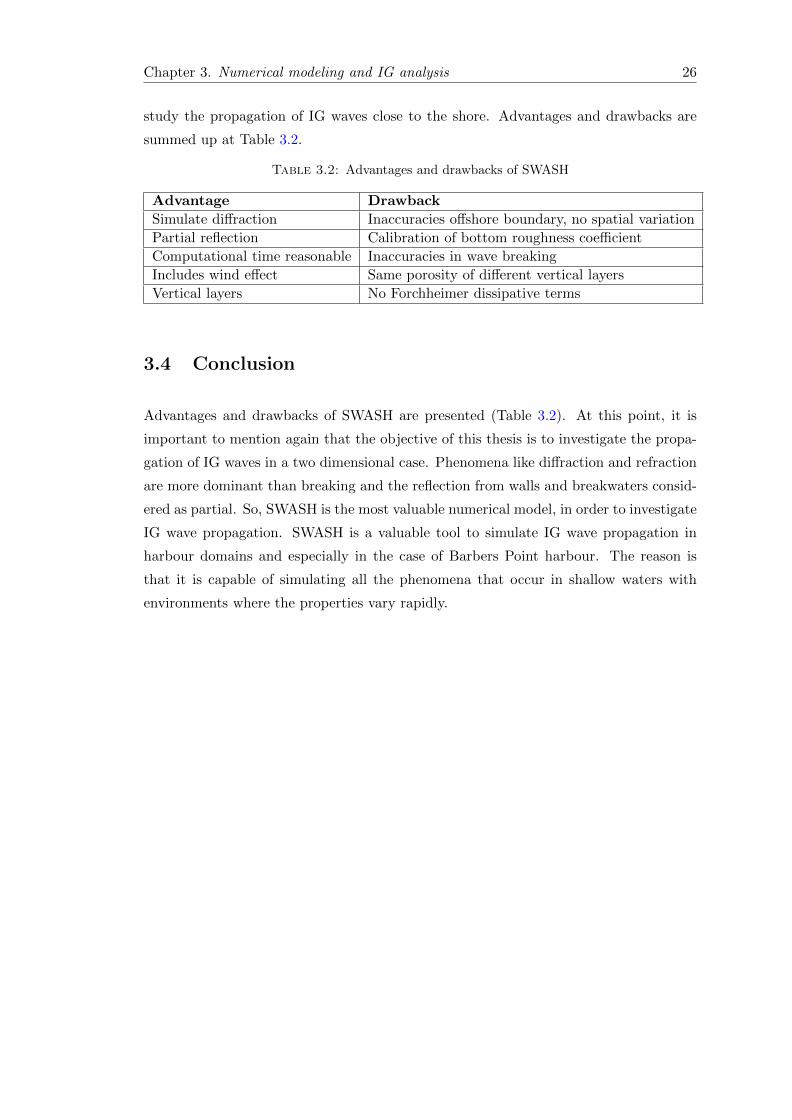
Barbers Point Harbour consists of by an entrance channel, a basin and a marina. The
entrance channel is 140m wide, 1000m long and approximately 13m deep. The depth of
the basin varies from 13.5−11.5m deep and it is 670m wide and 610m long, covering an
area of 0.4km2. The private marina is 67m by 400m and the mean depth is 7m. Rubble-
mound wave absorbers line 1400 linear meters of the inner shoreline of the harbour basin.
Figure 4.2 shows a plan view of the near-shore profile at the Barbers Point Harbour
area (including the basin and the private marina). The bathymetry is obtained by
Zeki Demirbilek during a survey conducted at 1995. The bathymetry characterized as
27
Chapter 4. The two-dimensional case: Barbers Point Harbour 28
uniform alongshore with steep slope in the offshore region (1:35) and mild slope in the
near-shore area (1:200).
Figure 4.2: A plan view and the bathymetry of Barbers Point harbour.
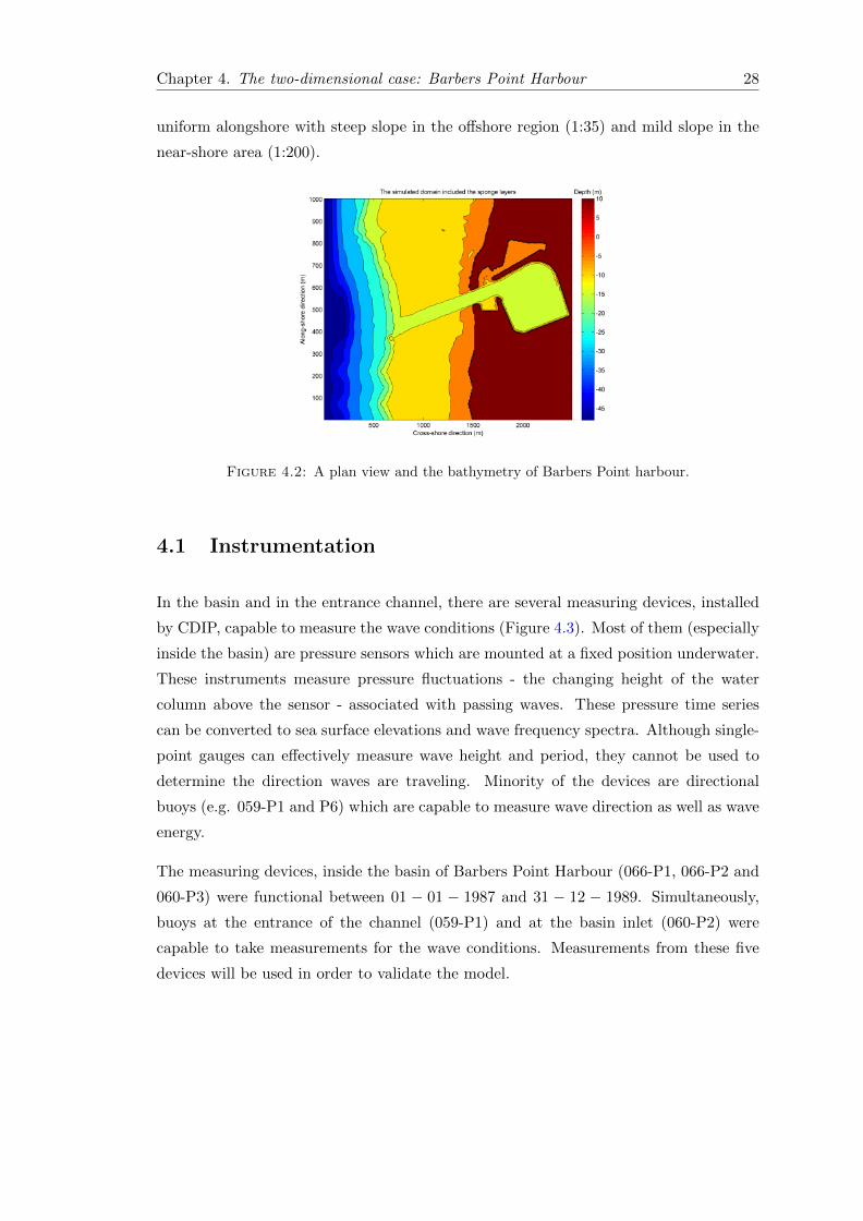
4.1 Instrumentation
In the basin and in the entrance channel, there are several measuring devices, installed
by CDIP, capable to measure the wave conditions (Figure 4.3). Most of them (especially
inside the basin) are pressure sensors which are mounted at a fixed position underwater.
These instruments measure pressure fluctuations - the changing height of the water
column above the sensor - associated with passing waves. These pressure time series
can be converted to sea surface elevations and wave frequency spectra. Although single-
point gauges can effectively measure wave height and period, they cannot be used to
determine the direction waves are traveling. Minority of the devices are directional
buoys (e.g. 059-P1 and P6) which are capable to measure wave direction as well as wave
energy.
The measuring devices, inside the basin of Barbers Point Harbour (066-P1, 066-P2 and
060-P3) were functional between 01 − 01 − 1987 and 31 − 12 − 1989. Simultaneously,
buoys at the entrance of the channel (059-P1) and at the basin inlet (060-P2) were
capable to take measurements for the wave conditions. Measurements from these five
devices will be used in order to validate the model.
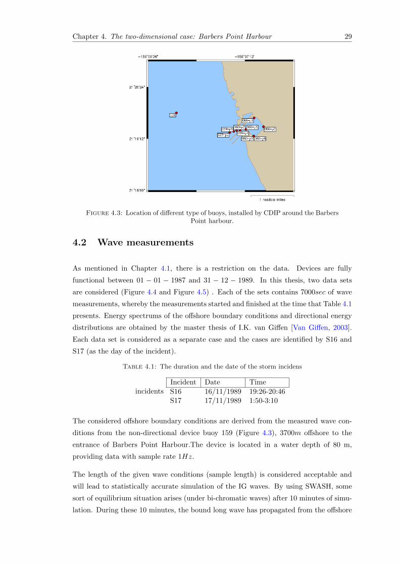
Chapter 4. The two-dimensional case: Barbers Point Harbour 29
Figure 4.3: Location of different type of buoys, installed by CDIP around the BarbersPoint harbour.
4.2 Wave measurements
As mentioned in Chapter 4.1, there is a restriction on the data. Devices are fully
functional between 01 − 01 − 1987 and 31 − 12 − 1989. In this thesis, two data sets
are considered (Figure 4.4 and Figure 4.5) . Each of the sets contains 7000sec of wave
measurements, whereby the measurements started and finished at the time that Table 4.1
presents. Energy spectrums of the offshore boundary conditions and directional energy
distributions are obtained by the master thesis of I.K. van Giffen [Van Giffen, 2003].
Each data set is considered as a separate case and the cases are identified by S16 and
S17 (as the day of the incident).
Table 4.1: The duration and the date of the storm incidens
incidentsIncident Date Time
S16 16/11/1989 19:26-20:46S17 17/11/1989 1:50-3:10
The considered offshore boundary conditions are derived from the measured wave con-
ditions from the non-directional device buoy 159 (Figure 4.3), 3700m offshore to the
entrance of Barbers Point Harbour.The device is located in a water depth of 80 m,
providing data with sample rate 1Hz.
The length of the given wave conditions (sample length) is considered acceptable and
will lead to statistically accurate simulation of the IG waves. By using SWASH, some
sort of equilibrium situation arises (under bi-chromatic waves) after 10 minutes of simu-
lation. During these 10 minutes, the bound long wave has propagated from the offshore

Chapter 4. The two-dimensional case: Barbers Point Harbour 30
Figure 4.4: Offshore boundary energy condition (buoy 159) during the storm of 16-11-1989, 19:30-20:45. Sample length is 3900 seconds,sample rate 1 Hz and the mean
direction is 260 degrees.
Figure 4.5: Offshore boundary energy condition (buoy 159) during the storm of 16-11-1989, 19:30-20:45. Sample length is 4800 seconds, sample rate 1 Hz and the mean
direction is 275 degrees.
boundary to the harbour, has traveled across the basin, has been released as free in-
fragravity wave and the equilibrium is arisen, as mentioned before. The length of the
measured data has to be 80 minutes (10 until the equilibrium and 70 for the IG simula-
tion) in order to achieve sufficient accuracy to enable high quality validation (simulate
more than 100 infragravity waves) of the model.
4.3 Other characteristics of the harbour
The reflection of the infragravity waves on the structures is important for the overall
wave pattern in the basin. In general, the reflected IG wave is considered much longer

Chapter 4. The two-dimensional case: Barbers Point Harbour 31
than the obstacle (which causes the reflection) so the reflection is assumed as full. It is
worth mentioning that this assumption will lead to overestimation for higher frequency
waves.
Not much is known about the bed material for Barbers Point Harbour. The type of
bottom material offshore is some sort of coral reef. For the case of Barbers Point
harbour, mild reflection is expected due to the mild slope of the adjacent shore and
bottom friction is not considered as a dominant dissipation mechanism for the incoming
IG waves. However, inaccuracies are expected on the calculations of the outgoing IG
waves as Rijnsdorp et al. [2014] identified.
Wave data was detrended over 1000sec intervals to remove tidal components. During
the first part of the storm the tide was subsiding. During the second part the tide was
at its lowest point. Tidal amplitude at the moment was around 0.35 cm. Because of this
low tidal amplitude the influence of the tide on the outcome of the model is not taken
into count. Slight errors in determined response frequencies could be the result of this
assumption.
Finally, the meteorological data for the two different incident storms, S16 and S17, are
given by the National Data Buoy Center. The wind regime is measured 70km away from
the Barbers point Harbour and it is shown in Table 4.2. The wind speeds, for both of
the cases, were remaining steady during the storm, according to the data provider.
Table 4.2: Wind speed during the investigated storms
Incident Date Wave speed (m/s)
S16 16/11/1989 11S17 17/11/1989 12
4.4 Infragravity wave regime
At the measuring location 059-P1, the given surface elevation is decomposed to the
IG wave and short wave component by using the FFT method. Aim is to present the
infragravity regime outside the basin and identify the origin of the IG waves. Insight to
the generation and propagation of the IG waves is given by using the cross-correlation
function and determine the ratio of the bound and free IG waves at the specific location
(059-P1).
As mentioned, surface elevation ζ is given at the buoy 059-P1. By using the frequency
band (0.005Hz < f < 0.05Hz) for the IG waves, ζIG and ζhf , for the IG waves and the
short waves respectively, are extracted. The forcing of the IG-waves are related with the
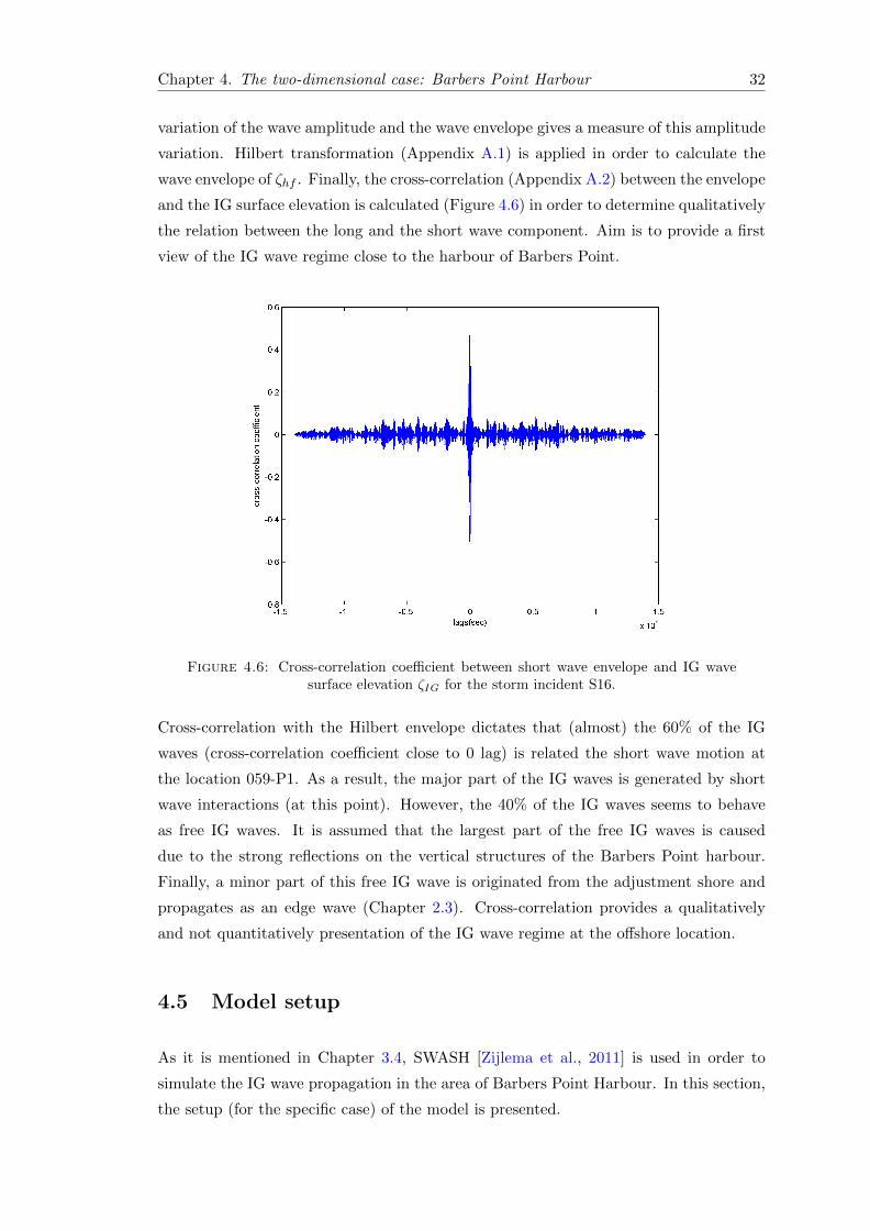
Chapter 4. The two-dimensional case: Barbers Point Harbour 32
variation of the wave amplitude and the wave envelope gives a measure of this amplitude
variation. Hilbert transformation (Appendix A.1) is applied in order to calculate the
wave envelope of ζhf . Finally, the cross-correlation (Appendix A.2) between the envelope
and the IG surface elevation is calculated (Figure 4.6) in order to determine qualitatively
the relation between the long and the short wave component. Aim is to provide a first
view of the IG wave regime close to the harbour of Barbers Point.
Figure 4.6: Cross-correlation coefficient between short wave envelope and IG wavesurface elevation ζIG for the storm incident S16.
Cross-correlation with the Hilbert envelope dictates that (almost) the 60% of the IG
waves (cross-correlation coefficient close to 0 lag) is related the short wave motion at
the location 059-P1. As a result, the major part of the IG waves is generated by short
wave interactions (at this point). However, the 40% of the IG waves seems to behave
as free IG waves. It is assumed that the largest part of the free IG waves is caused
due to the strong reflections on the vertical structures of the Barbers Point harbour.
Finally, a minor part of this free IG wave is originated from the adjustment shore and
propagates as an edge wave (Chapter 2.3). Cross-correlation provides a qualitatively
and not quantitatively presentation of the IG wave regime at the offshore location.
4.5 Model setup
As it is mentioned in Chapter 3.4, SWASH [Zijlema et al., 2011] is used in order to
simulate the IG wave propagation in the area of Barbers Point Harbour. In this section,
the setup (for the specific case) of the model is presented.
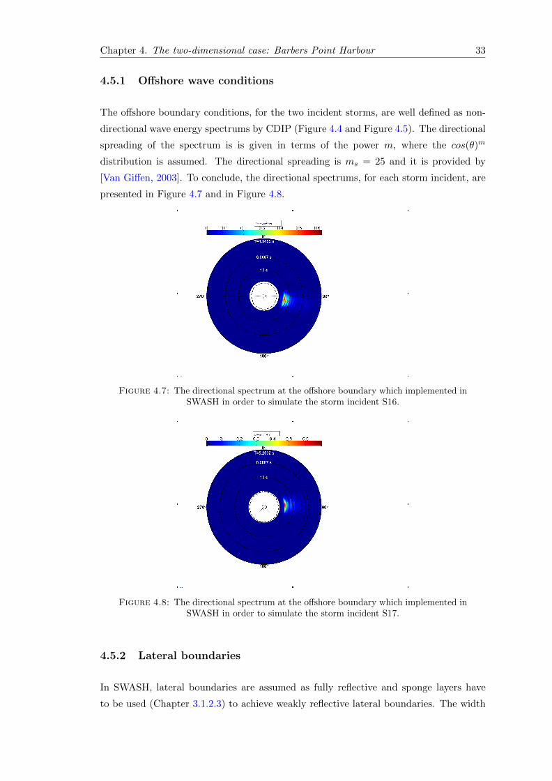
Chapter 4. The two-dimensional case: Barbers Point Harbour 33
4.5.1 Offshore wave conditions
The offshore boundary conditions, for the two incident storms, are well defined as non-
directional wave energy spectrums by CDIP (Figure 4.4 and Figure 4.5). The directional
spreading of the spectrum is is given in terms of the power m, where the cos(θ)m
distribution is assumed. The directional spreading is ms = 25 and it is provided by
[Van Giffen, 2003]. To conclude, the directional spectrums, for each storm incident, are
presented in Figure 4.7 and in Figure 4.8.
Figure 4.7: The directional spectrum at the offshore boundary which implemented inSWASH in order to simulate the storm incident S16.
Figure 4.8: The directional spectrum at the offshore boundary which implemented inSWASH in order to simulate the storm incident S17.
4.5.2 Lateral boundaries
In SWASH, lateral boundaries are assumed as fully reflective and sponge layers have
to be used (Chapter 3.1.2.3) to achieve weakly reflective lateral boundaries. The width
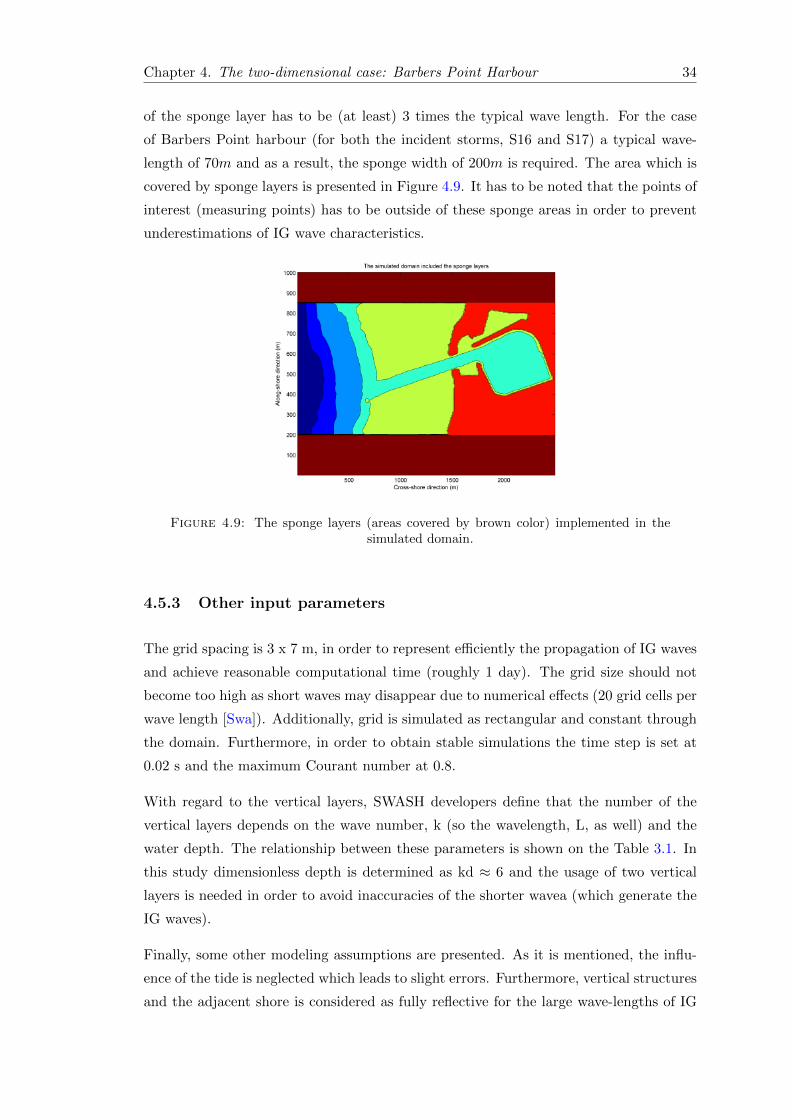
Chapter 4. The two-dimensional case: Barbers Point Harbour 34
of the sponge layer has to be (at least) 3 times the typical wave length. For the case
of Barbers Point harbour (for both the incident storms, S16 and S17) a typical wave-
length of 70m and as a result, the sponge width of 200m is required. The area which is
covered by sponge layers is presented in Figure 4.9. It has to be noted that the points of
interest (measuring points) has to be outside of these sponge areas in order to prevent
underestimations of IG wave characteristics.
Figure 4.9: The sponge layers (areas covered by brown color) implemented in thesimulated domain.
4.5.3 Other input parameters
The grid spacing is 3 x 7 m, in order to represent efficiently the propagation of IG waves
and achieve reasonable computational time (roughly 1 day). The grid size should not
become too high as short waves may disappear due to numerical effects (20 grid cells per
wave length [Swa]). Additionally, grid is simulated as rectangular and constant through
the domain. Furthermore, in order to obtain stable simulations the time step is set at
0.02 s and the maximum Courant number at 0.8.
With regard to the vertical layers, SWASH developers define that the number of the
vertical layers depends on the wave number, k (so the wavelength, L, as well) and the
water depth. The relationship between these parameters is shown on the Table 3.1. In
this study dimensionless depth is determined as kd ≈ 6 and the usage of two vertical
layers is needed in order to avoid inaccuracies of the shorter wavea (which generate the
IG waves).
Finally, some other modeling assumptions are presented. As it is mentioned, the influ-
ence of the tide is neglected which leads to slight errors. Furthermore, vertical structures
and the adjacent shore is considered as fully reflective for the large wave-lengths of IG

Chapter 4. The two-dimensional case: Barbers Point Harbour 35
waves. Additionally, the minimum simulated depth is considered as 0.3 m in order to
prevent instabilities. This characteristic has no effect inside the basin (or outside) but
it will lead to inaccuracies close to the shore-line.

Chapter 5
Sensitivity analysis and model
validation
As it is mentioned, the input data (offshore wave conditions) for modeling are provided,
partially from the CDIP and by [Van Giffen, 2003]. In order to proceed, the rest of the
input data (offshore directional spreading and model setup parameters) are calculated
and their sensitivity on the calculations are determined in Chapter 5. The effect of the
parameters in Table 5.1 tuning is tested in SWASH. The tuned characteristics of the
IG waves (in terms of wave energy spectrum and significant wave height, HIG,sig) are
compared with the observed IG wave measurements at the location 059-P1, outside of
the basin (Figure 4.3). The comparison is carried out for the frequency band of the IG
long waves (0.005 Hz- 0.05 Hz). After the determination of the Table 5.1 parameters,
the IG wave behavior is presented and compared with the measured one inside the
basin. Finally, the predictive skill of SWASH is calculated. In Chapter 5, the sensitivity
analysis and validation is carried out only for the wave condition S16, whereas results
for the wave condition S17 are presented in Appendix B.
5.1 Sensitivity Analysis
Despite the amount of data which are provided by CDIP and [Van Giffen, 2003], there
are some input modeling parameters which are unknown a priori. These parameters
are presented in Table 5.1 and they lead to simulation uncertainties. The sensitivity of
SWASH will be investigated only for the parameters/ characteristics:
1. Directional Spreading, ms
36
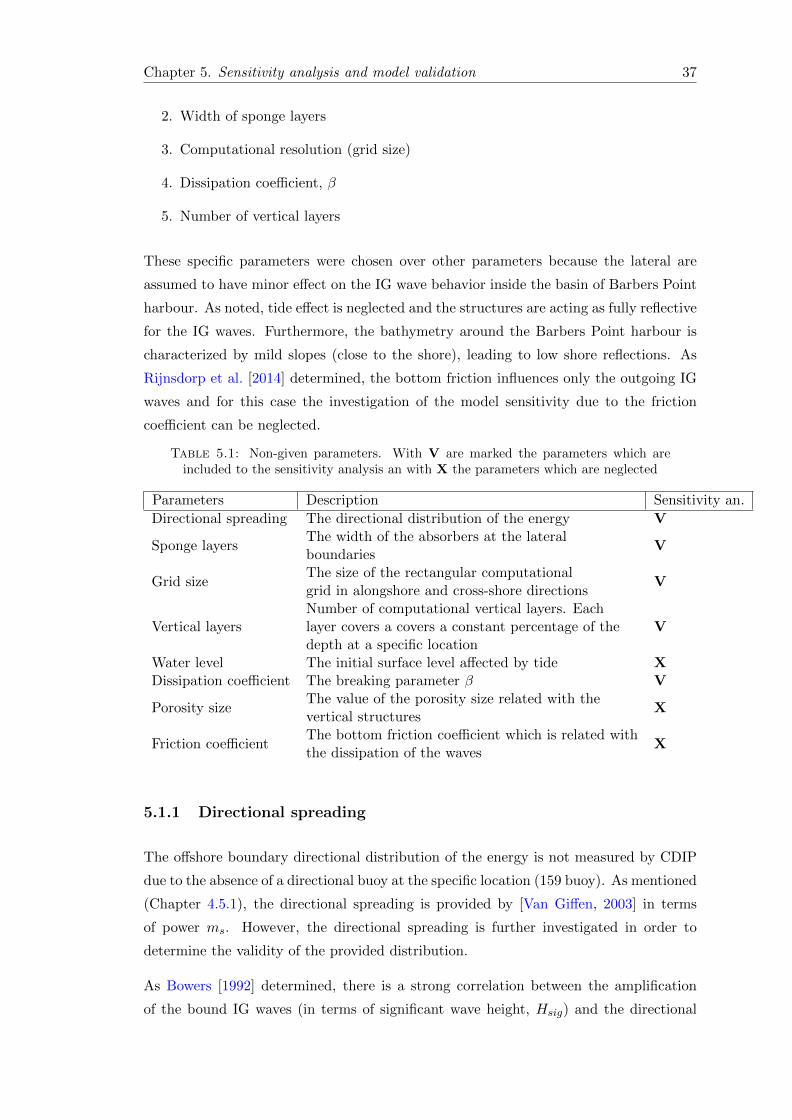
Chapter 5. Sensitivity analysis and model validation 37
2. Width of sponge layers
3. Computational resolution (grid size)
4. Dissipation coefficient, β
5. Number of vertical layers
These specific parameters were chosen over other parameters because the lateral are
assumed to have minor effect on the IG wave behavior inside the basin of Barbers Point
harbour. As noted, tide effect is neglected and the structures are acting as fully reflective
for the IG waves. Furthermore, the bathymetry around the Barbers Point harbour is
characterized by mild slopes (close to the shore), leading to low shore reflections. As
Rijnsdorp et al. [2014] determined, the bottom friction influences only the outgoing IG
waves and for this case the investigation of the model sensitivity due to the friction
coefficient can be neglected.
Table 5.1: Non-given parameters. With V are marked the parameters which areincluded to the sensitivity analysis an with X the parameters which are neglected
Parameters Description Sensitivity an.
Directional spreading The directional distribution of the energy V
Sponge layersThe width of the absorbers at the lateralboundaries
V
Grid sizeThe size of the rectangular computationalgrid in alongshore and cross-shore directions
V
Vertical layersNumber of computational vertical layers. Eachlayer covers a covers a constant percentage of thedepth at a specific location
V
Water level The initial surface level affected by tide XDissipation coefficient The breaking parameter β V
Porosity sizeThe value of the porosity size related with thevertical structures
X
Friction coefficientThe bottom friction coefficient which is related withthe dissipation of the waves
X
5.1.1 Directional spreading
The offshore boundary directional distribution of the energy is not measured by CDIP
due to the absence of a directional buoy at the specific location (159 buoy). As mentioned
(Chapter 4.5.1), the directional spreading is provided by [Van Giffen, 2003] in terms
of power ms. However, the directional spreading is further investigated in order to
determine the validity of the provided distribution.
As Bowers [1992] determined, there is a strong correlation between the amplification
of the bound IG waves (in terms of significant wave height, Hsig) and the directional

Chapter 5. Sensitivity analysis and model validation 38
spreading. Bowers [1992] proved that the spreading is disproportional with the height
and the length of the bound IG waves.
Figure 5.1: The IG wave energy spectrum for different values of directional spreadingat the location 059-P1. Blue is the measured form CDIP, green for ms=10, red for
ms=15, cyan for ms=20, magenta for ms=25 and yellow for ms=40.
Table 5.2: The IG wave significant height for different directional spreading valuescompared to the observed one.
Directional spreading, ms Significant IG wave height, HIG,sig (m)
Observed 0.2310 0.2015 0.2120 0.2125 0.2240 0.26
As it was expected, the IG wave significant height, HIG,sig, decreases as the spreading
increases (ms decreases). Figure 5.1 shows that directional spreading has a strong effect
to the increase of the IG wave energy at the location 059-P1. The observed IG wave
significant height,HIG,sig, is 0.23m. So, this research agrees with [Van Giffen, 2003] that
a reasonable value for the directional spreading is ms = 25. Slight mismatching, between
the observed spectrum and the calculated for the ms = 25, is caused because of these
following reasons:
1. The IG wave frequencies lie below the conventional range of commonly deployed
wave measurement devices
2. The location of the buoy 059-P1 is not provided but it is approximated from
Figure 4.3
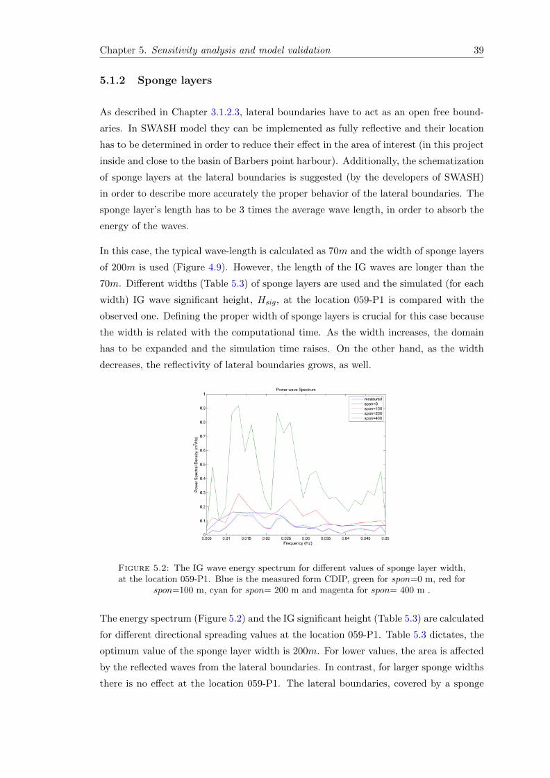
Chapter 5. Sensitivity analysis and model validation 39
5.1.2 Sponge layers
As described in Chapter 3.1.2.3, lateral boundaries have to act as an open free bound-
aries. In SWASH model they can be implemented as fully reflective and their location
has to be determined in order to reduce their effect in the area of interest (in this project
inside and close to the basin of Barbers point harbour). Additionally, the schematization
of sponge layers at the lateral boundaries is suggested (by the developers of SWASH)
in order to describe more accurately the proper behavior of the lateral boundaries. The
sponge layer’s length has to be 3 times the average wave length, in order to absorb the
energy of the waves.
In this case, the typical wave-length is calculated as 70m and the width of sponge layers
of 200m is used (Figure 4.9). However, the length of the IG waves are longer than the
70m. Different widths (Table 5.3) of sponge layers are used and the simulated (for each
width) IG wave significant height, Hsig, at the location 059-P1 is compared with the
observed one. Defining the proper width of sponge layers is crucial for this case because
the width is related with the computational time. As the width increases, the domain
has to be expanded and the simulation time raises. On the other hand, as the width
decreases, the reflectivity of lateral boundaries grows, as well.
Figure 5.2: The IG wave energy spectrum for different values of sponge layer width,at the location 059-P1. Blue is the measured form CDIP, green for spon=0 m, red for
spon=100 m, cyan for spon= 200 m and magenta for spon= 400 m .
The energy spectrum (Figure 5.2) and the IG significant height (Table 5.3) are calculated
for different directional spreading values at the location 059-P1. Table 5.3 dictates, the
optimum value of the sponge layer width is 200m. For lower values, the area is affected
by the reflected waves from the lateral boundaries. In contrast, for larger sponge widths
there is no effect at the location 059-P1. The lateral boundaries, covered by a sponge
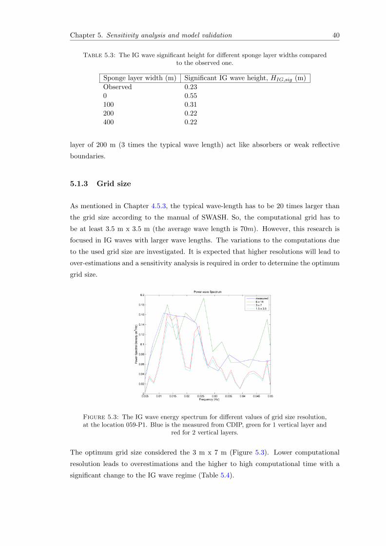
Chapter 5. Sensitivity analysis and model validation 40
Table 5.3: The IG wave significant height for different sponge layer widths comparedto the observed one.
Sponge layer width (m) Significant IG wave height, HIG,sig (m)
Observed 0.230 0.55100 0.31200 0.22400 0.22
layer of 200 m (3 times the typical wave length) act like absorbers or weak reflective
boundaries.
5.1.3 Grid size
As mentioned in Chapter 4.5.3, the typical wave-length has to be 20 times larger than
the grid size according to the manual of SWASH. So, the computational grid has to
be at least 3.5 m x 3.5 m (the average wave length is 70m). However, this research is
focused in IG waves with larger wave lengths. The variations to the computations due
to the used grid size are investigated. It is expected that higher resolutions will lead to
over-estimations and a sensitivity analysis is required in order to determine the optimum
grid size.
Figure 5.3: The IG wave energy spectrum for different values of grid size resolution,at the location 059-P1. Blue is the measured from CDIP, green for 1 vertical layer and
red for 2 vertical layers.
The optimum grid size considered the 3 m x 7 m (Figure 5.3). Lower computational
resolution leads to overestimations and the higher to high computational time with a
significant change to the IG wave regime (Table 5.4).

Chapter 5. Sensitivity analysis and model validation 41
Table 5.4: The IG wave significant height for different grid sizes compared to theobserved one.
Grid size ( Alongshore direction x Cross-shore direction) Significant IG wave height, HIG,sig (m)
Observed 0.236 m x 14 m 0.553 m x 7 m 0.311.5 m x 3.5 m 0.22
5.1.4 Vertical layers
The vertical separation of the domain in layers is the innovative feature of SWASH
compared to the other wave numerical tools. As defined in Chapter 4.5.3, the vertical
layers has to be 2 in in order to prevent inaccuracies in depths larger than 30m. At
this high-depth locations the waves interacting between its other but the ”strength” of
these interactions are low. The amplification of bound IG waves becomes significant
when the wave group propagates through depths lower than 15 m, where the use of one
vertical layer is considered reasonable. Fluctuations of the IG wave calculations (at the
measured locations) due to the number of vertical layers are determined for the case
of Barbers Point harbour. Unfortunately, SWASH becomes unstable when the vertical
domain is separated in 3 layers, especially close to the structures.
Figure 5.4: The IG wave energy spectrum for different number of vertical layers, atthe location 059-P1. Blue is the measured form CDIP, green for 1 vertical layer and
red for 2 vertical layers.
Table 5.5: The IG wave significant height for different grid sizes compared to theobserved one.
Number of vertical layers Significant IG wave height, HIG,sig (m)
Observed 0.231 vertical layer 0.282 vertical layers 0.22

Chapter 5. Sensitivity analysis and model validation 42
At this point, it has to be mentioned that the number of vertical layers is related with
the computational resolution, similar to the the grid size. As explained in the previous
Chapter 5.1.3, when the resolution becomes coarser, SWASH tends to overestimate the
characteristics of the IG wave (Figure 5.4 and Table 5.5).
5.1.5 Breaking parameter
The default value dissipation coefficient, α, which controls the wave breaking is 0.6 and
it is considered reasonable both for irregular and regular waves over mild bathymetries.
However, for steep bathymetries the value of β has to be reduced. In the case of a
harbour, breaking phenomenon is not significant. However, there is a possibility to have
significant contribution to the IG wave energy by edge waves (Chapter 2.3) which are
related to the breaking phenomenon and generated at the adjacent beach.
Figure 5.5: The IG wave energy spectrum for different dissipation coefficient, at thelocation 059-P1. Blue is the measured form CDIP, green for α = 0.4 and red for α = 0.6
Table 5.6: The IG wave significant height for different grid sizes compared to theobserved one.
Dissipation coefficient, α Significant IG wave height, HIG,sig (m)
Observed 0.230.4 0.310.6 0.22
Reduction of the breaking parameter β leads to overestimation of the IG wave energy
density (spectrum) (Figure 5.5) and the IG significant height (Table 5.6). The short
waves tend to break earlier, the surf zone expands and the edge waves are amplified.
This phenomenon increases the IG wave height, HIG,sig at the location 059-P1.
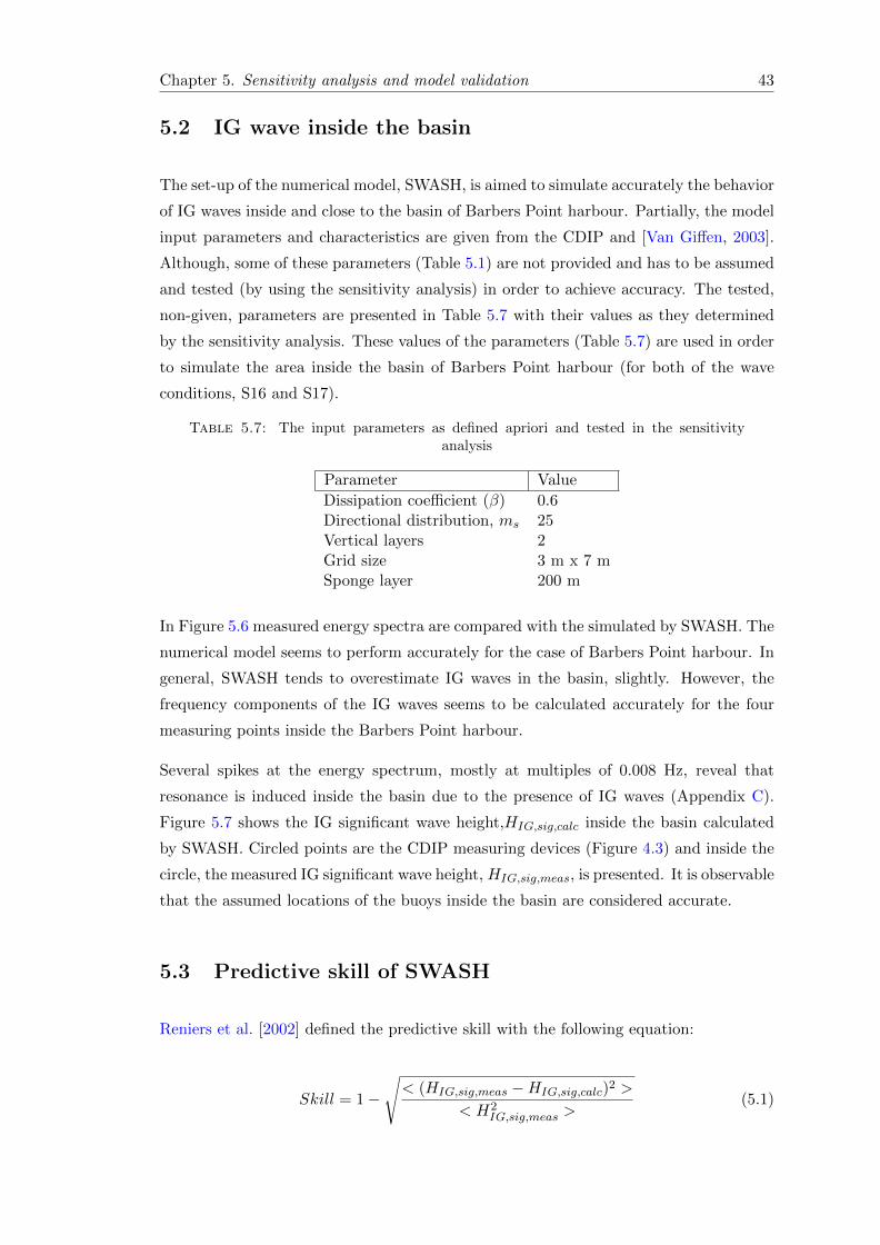
Chapter 5. Sensitivity analysis and model validation 43
5.2 IG wave inside the basin
The set-up of the numerical model, SWASH, is aimed to simulate accurately the behavior
of IG waves inside and close to the basin of Barbers Point harbour. Partially, the model
input parameters and characteristics are given from the CDIP and [Van Giffen, 2003].
Although, some of these parameters (Table 5.1) are not provided and has to be assumed
and tested (by using the sensitivity analysis) in order to achieve accuracy. The tested,
non-given, parameters are presented in Table 5.7 with their values as they determined
by the sensitivity analysis. These values of the parameters (Table 5.7) are used in order
to simulate the area inside the basin of Barbers Point harbour (for both of the wave
conditions, S16 and S17).
Table 5.7: The input parameters as defined apriori and tested in the sensitivityanalysis
Parameter Value
Dissipation coefficient (β) 0.6Directional distribution, ms 25Vertical layers 2Grid size 3 m x 7 mSponge layer 200 m
In Figure 5.6 measured energy spectra are compared with the simulated by SWASH. The
numerical model seems to perform accurately for the case of Barbers Point harbour. In
general, SWASH tends to overestimate IG waves in the basin, slightly. However, the
frequency components of the IG waves seems to be calculated accurately for the four
measuring points inside the Barbers Point harbour.
Several spikes at the energy spectrum, mostly at multiples of 0.008 Hz, reveal that
resonance is induced inside the basin due to the presence of IG waves (Appendix C).
Figure 5.7 shows the IG significant wave height,HIG,sig,calc inside the basin calculated
by SWASH. Circled points are the CDIP measuring devices (Figure 4.3) and inside the
circle, the measured IG significant wave height, HIG,sig,meas, is presented. It is observable
that the assumed locations of the buoys inside the basin are considered accurate.
5.3 Predictive skill of SWASH
Reniers et al. [2002] defined the predictive skill with the following equation:
Skill = 1−√< (HIG,sig,meas −HIG,sig,calc)2 >
< H2IG,sig,meas >
(5.1)
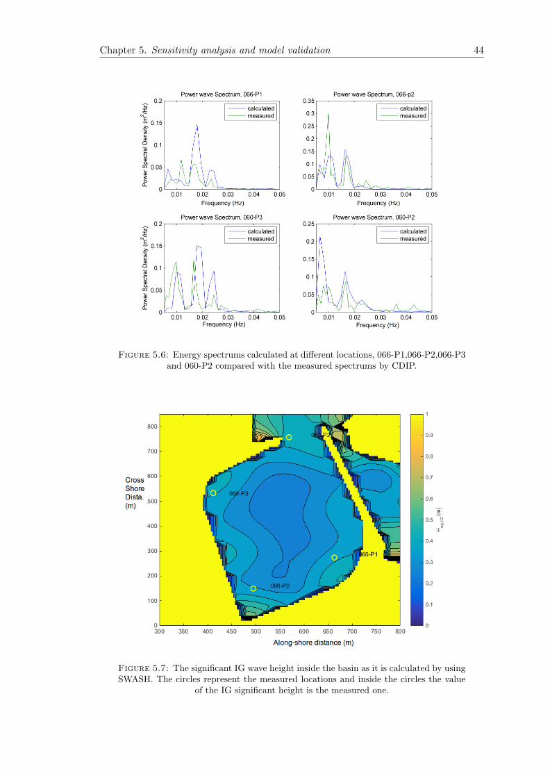
Chapter 5. Sensitivity analysis and model validation 44
Figure 5.6: Energy spectrums calculated at different locations, 066-P1,066-P2,066-P3and 060-P2 compared with the measured spectrums by CDIP.
Figure 5.7: The significant IG wave height inside the basin as it is calculated by usingSWASH. The circles represent the measured locations and inside the circles the value
of the IG significant height is the measured one.

Chapter 5. Sensitivity analysis and model validation 45
HIG,sig,meas is the measured significant height andHIG,sig,calc is the calculated significant
IG wave height. The predictive skill gives an indication of the magnitude of the difference
between the measurements and the predictions relative to the measured value. For a skill
of 1 the difference is zero, while for a value of 0 the difference is equal to the measured
value. The results show that SWASH is capable of predicting the IG-wave conditions
at a specific site with an average skill of 0.84. The predictive skill is 5 % higher than
Reniers et al. [2010] and Rijnsdorp [2011] calculated by using IDSB [Reniers et al., 2002]
and SWASH respectively. It was expected a high predictive skill of the numerical model,
due to the usage (for this project) of the newest (2.00) and more validated version of
SWASH.

Chapter 6
Separation of the Infragravity
waves
As mentioned in Chapter 1 and Chapter 2, IG waves are generated by non-linear in-
teractions of short waves in the shoaling area (seawards of the breaking zone). Going
deeper, to the field of IG wave origins, Longuet-Higgins and Stewart [1962] identified
that a pair of short waves with relatively close frequencies, f1 and f2, tends to generate
a bound and ”out of phase” wave with frequency, f1 − f2, due to mass and momentum
fluxes modulations with the short wave groups.
Bispectral analysis is a valuable tool in order to investigate the boundness between the
short and the IG waves (Chapter 3.2). In this thesis, measurements of surface elevation
(at several locations) are used to obtain the linear, the non-linear energy fluxes and the
energy transfers between the short and IG waves based on the equations of Ruessink
[1998](Chapter 3.2). Additionally, the IG wave signal is decomposed to the incoming
and outgoing component by using the Sheremet et al. [2002] method (Chapter 2.3).
6.1 Methodology
6.1.1 Description of the domain and the wave conditions
The investigated domain is the Barbers Point Harbour (Figure 4.2). The offshore wave
condition is the storm on 16 of November 1988, presented in Chapter 4.2. Focus is
given on one offshore wave condition (S16) in order to understand and analyze in depth
the IG wave complex behavior. Finally, the numerical model (SWASH) set-up remains
the same as it was determined partially in Chapter 4 and, after an extensive sensitivity
analysis, in Chapter 5.
46
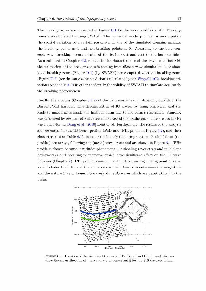
Chapter 6. Separation of the Infragravity waves 47
The breaking zones are presented in Figure D.1 for the wave conditions S16. Breaking
zones are calculated by using SWASH. The numerical model provide (as an output) a
the spatial variation of a certain parameter in the of the simulated domain, masking
the breaking points as 1 and non-breaking points as 0. According to the bore con-
cept, wave breaking occurs outside of the basin, west and east to the harbour inlet.
As mentioned in Chapter 4.2, related to the characteristics of the wave condition S16,
the estimation of the breaker zones is coming from 65min wave simulation. The simu-
lated breaking zones (Figure D.1) (by SWASH) are compared with the breaking zones
(Figure D.2) (for the same wave conditions) calculated by the Weggel [1972] breaking cri-
terion (Appendix A.3) in order to identify the validity of SWASH to simulate accurately
the breaking phenomenon.
Finally, the analysis (Chapter 6.1.2) of the IG waves is taking place only outside of the
Barber Point harbour. The decomposition of IG waves, by using bispectral analysis,
leads to inaccuracies inside the harbour basin due to the basin’s resonance. Standing
waves (caused by resonance) will cause an increase of the bicoherence, unrelated to the IG
wave behavior, as Dong et al. [2010] mentioned. Furthermore, the results of the analysis
are presented for two 1D beach profiles (PBr and PIn profile in Figure 6.2), and their
characteristics at Table 6.1), in order to simplify the interpretation. Both of them (the
profiles) are arrays, following the (mean) wave crests and are shown in Figure 6.1. PBr
profile is chosen because it includes phenomena like shoaling (over steep and mild slope
bathymetry) and breaking phenomena, which have significant effect on the IG wave
behavior (Chapter 2). PIn profile is more important from an engineering point of view,
as it includes the inlet and the entrance channel. Aim is to determine the magnitude
and the nature (free or bound IG waves) of the IG waves which are penetrating into the
basin.
Figure 6.1: Location of the simulated transects, PBr (blue ) and PIn (green). Arrowsshow the mean direction of the waves (total wave signal) for the S16 wave condition.

Chapter 6. Separation of the Infragravity waves 48
Figure 6.2: The bottom profiles, PBr (upper panel) and PIn (bottom panel). Withred color is the bottom profile and with blue the mean water level.
SimulatedProfile
DiscreteZones
Cross-shoreDistance (m)
SimulatedProfile
DiscreteZones
Cross-shoreDistance (m)
PBr Steep-slope 0 -600 PIn Steep-slope 0 -600
Mild-slope 600 -1200EntranceChannel
600 -1400
Offshore to thebreaking point
1200 -1300Close tothe inlet
1400 -1500
Breaking zone 1300 -1400Surf Zone 1400 -1500
Table 6.1: Separation of the profiles PBr and PIn to discrete zones
6.1.2 Analysis
The first objective of the IG wave analysis is to separate the low from the high frequency
signal (Chapter 6.2.1). The FFT method (Chapter 3.2) is applied to the surface elevation
signal (recording frequency, f = 10Hz) and frequency band filters are applied (IG
waves frequency between 0.005-0.05 Hz and short wave frequency between 0.05-0.25
Hz). A separation of the high-low signal and calculation of their characteristics (i.e.
Hsig, energy) shows the origin and the propagation of the IG waves.
One step forward to this analysis is the decomposition of the IG wave signal (Chap-
ter 6.2.2). As mentioned in Chapter 1 and Chapter 2, IG waves are consisted by two
components, the bounded and the released (free) and for their decomposition, the bis-
pectral analysis is used. The frequency bispectral resolution is 0.0003Hz and the time
series are segmented in 1000s, 50% overlapping sections, that are detrended and ta-
pered by using the Hanning window. Double integration (between the IG and the short
wave frequency bands) of bicoherence determines the ratio of the bounded IG waves
(Chapter 3.2).
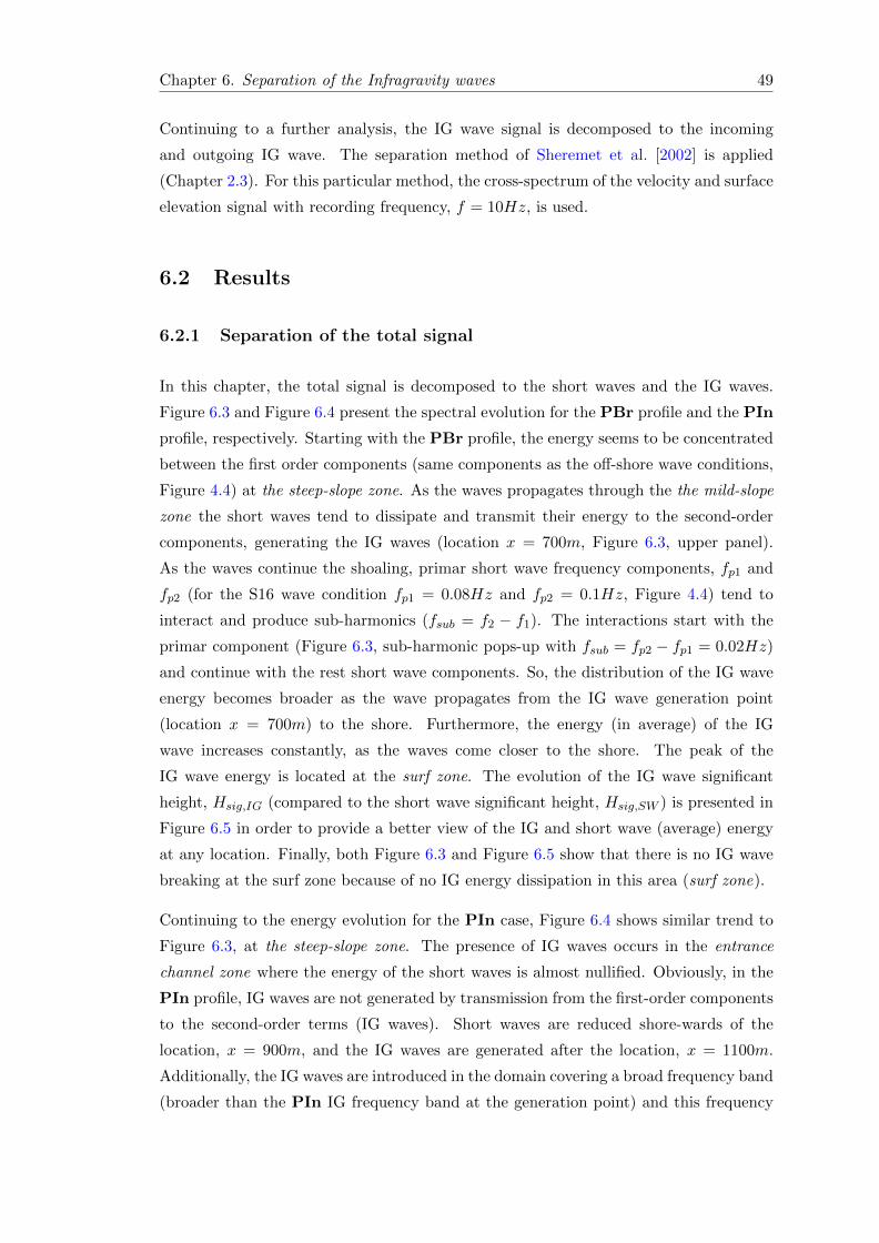
Chapter 6. Separation of the Infragravity waves 49
Continuing to a further analysis, the IG wave signal is decomposed to the incoming
and outgoing IG wave. The separation method of Sheremet et al. [2002] is applied
(Chapter 2.3). For this particular method, the cross-spectrum of the velocity and surface
elevation signal with recording frequency, f = 10Hz, is used.
6.2 Results
6.2.1 Separation of the total signal
In this chapter, the total signal is decomposed to the short waves and the IG waves.
Figure 6.3 and Figure 6.4 present the spectral evolution for the PBr profile and the PIn
profile, respectively. Starting with the PBr profile, the energy seems to be concentrated
between the first order components (same components as the off-shore wave conditions,
Figure 4.4) at the steep-slope zone. As the waves propagates through the the mild-slope
zone the short waves tend to dissipate and transmit their energy to the second-order
components, generating the IG waves (location x = 700m, Figure 6.3, upper panel).
As the waves continue the shoaling, primar short wave frequency components, fp1 and
fp2 (for the S16 wave condition fp1 = 0.08Hz and fp2 = 0.1Hz, Figure 4.4) tend to
interact and produce sub-harmonics (fsub = f2 − f1). The interactions start with the
primar component (Figure 6.3, sub-harmonic pops-up with fsub = fp2 − fp1 = 0.02Hz)
and continue with the rest short wave components. So, the distribution of the IG wave
energy becomes broader as the wave propagates from the IG wave generation point
(location x = 700m) to the shore. Furthermore, the energy (in average) of the IG
wave increases constantly, as the waves come closer to the shore. The peak of the
IG wave energy is located at the surf zone. The evolution of the IG wave significant
height, Hsig,IG (compared to the short wave significant height, Hsig,SW ) is presented in
Figure 6.5 in order to provide a better view of the IG and short wave (average) energy
at any location. Finally, both Figure 6.3 and Figure 6.5 show that there is no IG wave
breaking at the surf zone because of no IG energy dissipation in this area (surf zone).
Continuing to the energy evolution for the PIn case, Figure 6.4 shows similar trend to
Figure 6.3, at the steep-slope zone. The presence of IG waves occurs in the entrance
channel zone where the energy of the short waves is almost nullified. Obviously, in the
PIn profile, IG waves are not generated by transmission from the first-order components
to the second-order terms (IG waves). Short waves are reduced shore-wards of the
location, x = 900m, and the IG waves are generated after the location, x = 1100m.
Additionally, the IG waves are introduced in the domain covering a broad frequency band
(broader than the PIn IG frequency band at the generation point) and this frequency

Chapter 6. Separation of the Infragravity waves 50
Figure 6.3: The spectral evolution, in terms of variance energy density (m2/Hz).The upper panel dictates the energy distribution for the IG waves, (0.005 − 0.05Hz),and the bottom panel the energy distribution for the short waves,(0.05−0.25Hz). Both
of the panels are showing the energy evolution for the profile PBr
band remains, relatively, constant through the domain. So, there is no transmission
to the sub-order harmonics similar to the PBr case. This dictates the generation and
amplification of the IG waves in areas outside of the presented, PIn, domain (the mild-
slope zone of the adjacent area). Finally, the sharp decrease in the short wave energy (
Figure 6.5, bottom panel) at the area x = 600 − 1000m is caused by refraction due to
the entrance channel. Short wave tends to leak through the sides of the channel to the
adjacent area, when the IG wave are strongly refracted into the channel.
Finally, the IG wave direction of propagation is compared to the direction of short waves
and it is presented in Apppendix D. The directional spectrums are constructed for the
low and the high frequency components, for different locations of both the profiles, PBr
and PIn.
6.2.2 Decomposition of IG waves
Bispectral analysis showed non-linear transfers of energy for both, PBr and PIn profiles.
These energy transmissions are amplified across the shoaling areas and reduced due
to breaking phenomena. Figure 6.6 shows an example of the normalized bispectrum
(bicoherence) at several locations. Normalized bispectrum examples are presented only
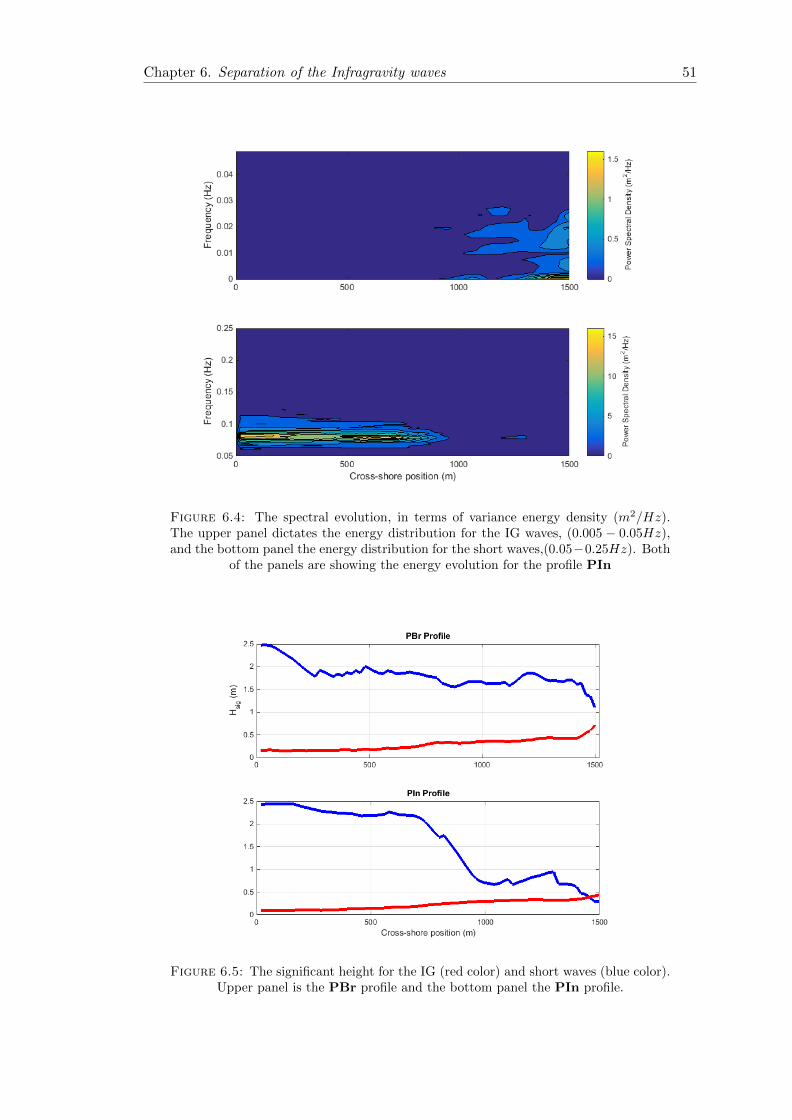
Chapter 6. Separation of the Infragravity waves 51
Figure 6.4: The spectral evolution, in terms of variance energy density (m2/Hz).The upper panel dictates the energy distribution for the IG waves, (0.005 − 0.05Hz),and the bottom panel the energy distribution for the short waves,(0.05−0.25Hz). Both
of the panels are showing the energy evolution for the profile PIn
Figure 6.5: The significant height for the IG (red color) and short waves (blue color).Upper panel is the PBr profile and the bottom panel the PIn profile.
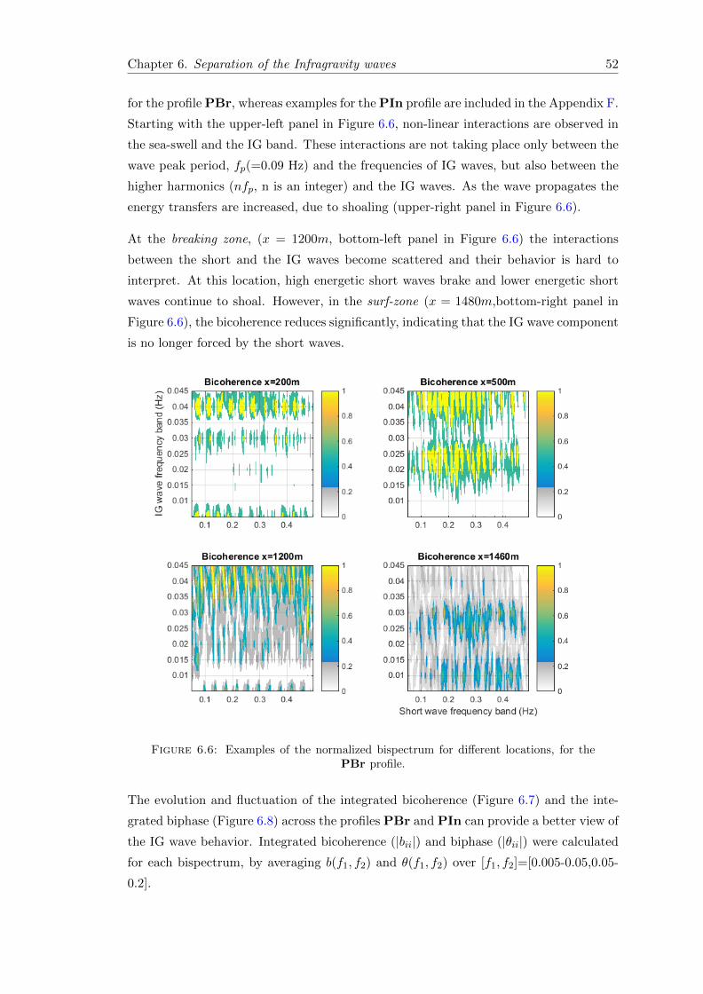
Chapter 6. Separation of the Infragravity waves 52
for the profile PBr, whereas examples for the PIn profile are included in the Appendix F.
Starting with the upper-left panel in Figure 6.6, non-linear interactions are observed in
the sea-swell and the IG band. These interactions are not taking place only between the
wave peak period, fp(=0.09 Hz) and the frequencies of IG waves, but also between the
higher harmonics (nfp, n is an integer) and the IG waves. As the wave propagates the
energy transfers are increased, due to shoaling (upper-right panel in Figure 6.6).
At the breaking zone, (x = 1200m, bottom-left panel in Figure 6.6) the interactions
between the short and the IG waves become scattered and their behavior is hard to
interpret. At this location, high energetic short waves brake and lower energetic short
waves continue to shoal. However, in the surf-zone (x = 1480m,bottom-right panel in
Figure 6.6), the bicoherence reduces significantly, indicating that the IG wave component
is no longer forced by the short waves.
Figure 6.6: Examples of the normalized bispectrum for different locations, for thePBr profile.
The evolution and fluctuation of the integrated bicoherence (Figure 6.7) and the inte-
grated biphase (Figure 6.8) across the profiles PBr and PIn can provide a better view of
the IG wave behavior. Integrated bicoherence (|bii|) and biphase (|θii|) were calculated
for each bispectrum, by averaging b(f1, f2) and θ(f1, f2) over [f1, f2]=[0.005-0.05,0.05-
0.2].
Chapter 6. Separation of the Infragravity waves 53
For both the profiles (PBr and PIn) the IG regime is similar at the steep-slope zone.
At the beginning, IG waves have low energy amplitude, due to the large depth, and are
continuing to shallower waters, where the bound IG waves are amplified. When the wave
is introduced to the mild-slope zone a decrease of the bicoherence occurs for both of the
cases. This behavior dictates a slight release of the IG waves due to the slope change.
The generation of free IG waves can be observed in Figure 6.7, as well (x = 550m).
For the PBr profile, the bicoherence remains steady as the toatal (IG and short) wave
propagates to the breaking zone. Close to the breaking point, bound IG wave seems
to be dominant (|bii| > 0.7). Moving further to the surf-zone the bicoherence drops
sharply, the biphase decreases and the bound IG waves are released. The boundness of
IG and short waves is slightly increased again in the shallower waters (1450 − 1500m)
of the surf-zone. The biphase (Figure 6.8, upper panel) remains constant (θ = 177o)
until the breaking point. Passing that point and reaching the breaking zone, the biphase
drops from θ = 177o to θ = 160o (in the surf zone), dictating the release of IG waves
due to breaking phenomena.
In contrast with PBr, PIn bicoherence does not show any severe fluctuations at the
entrance channel zone. The reason for that steady (b = 0.32 − 0.36) behavior is the
flat bathymetry. Only after x = 900m bicoherence drops by 0.1 and reaches again the
previous (b = 0.32−0.36) value after x = 1400m. This fluctuation is caused by the effect
of refraction, due to the entrance channel. Long waves are strongly refracted inside the
basin when the short waves propagate to the adjacent shore. This phenomenon cause
the release of IG waves and the slight drop of the bicoherence.
Finally, the free and bounded IG wave components are presented, in terms of significant
height ( Figure 6.9). For the PBr profile the maximum significant height of the bounded
component varies from 0.1m (offshore) to 0.2m (before the breaking occurs and close
to the shore). The free component becomes significant (Hsig,free < 0.1m) close to the
breaking zone and in the surf zone. For the PIn profile, both bound and free components
have a constant growth rate through the domain, reaching the maximum value at the
inlet (Hsig,boun = 0.15m and Hsig,free = 0.2m).
6.2.3 Reflection analysis
Further analysis includes the separation of the free IG wave to the components (in terms
of fluxes):
1. Incoming IG wave

Chapter 6. Separation of the Infragravity waves 54
Figure 6.7: Bicoherence, b, for the PBr profile (upper panel) and the PIn profile(bottom panel).
Figure 6.8: The simulated biphase, θ for the PBr profile (upper panel) and the PInprofile (bottom panel).
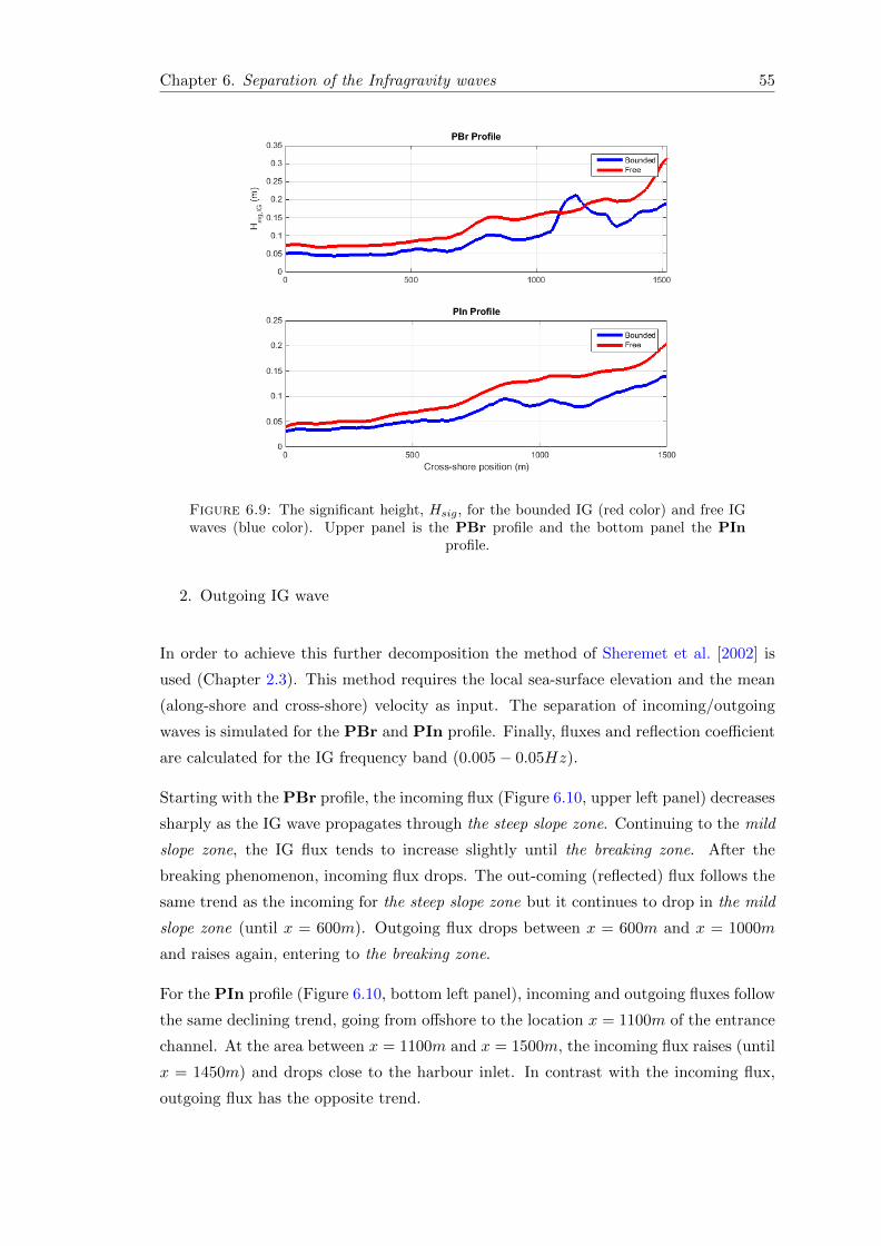
Chapter 6. Separation of the Infragravity waves 55
Figure 6.9: The significant height, Hsig, for the bounded IG (red color) and free IGwaves (blue color). Upper panel is the PBr profile and the bottom panel the PIn
profile.
2. Outgoing IG wave
In order to achieve this further decomposition the method of Sheremet et al. [2002] is
used (Chapter 2.3). This method requires the local sea-surface elevation and the mean
(along-shore and cross-shore) velocity as input. The separation of incoming/outgoing
waves is simulated for the PBr and PIn profile. Finally, fluxes and reflection coefficient
are calculated for the IG frequency band (0.005− 0.05Hz).
Starting with the PBr profile, the incoming flux (Figure 6.10, upper left panel) decreases
sharply as the IG wave propagates through the steep slope zone. Continuing to the mild
slope zone, the IG flux tends to increase slightly until the breaking zone. After the
breaking phenomenon, incoming flux drops. The out-coming (reflected) flux follows the
same trend as the incoming for the steep slope zone but it continues to drop in the mild
slope zone (until x = 600m). Outgoing flux drops between x = 600m and x = 1000m
and raises again, entering to the breaking zone.
For the PIn profile (Figure 6.10, bottom left panel), incoming and outgoing fluxes follow
the same declining trend, going from offshore to the location x = 1100m of the entrance
channel. At the area between x = 1100m and x = 1500m, the incoming flux raises (until
x = 1450m) and drops close to the harbour inlet. In contrast with the incoming flux,
outgoing flux has the opposite trend.
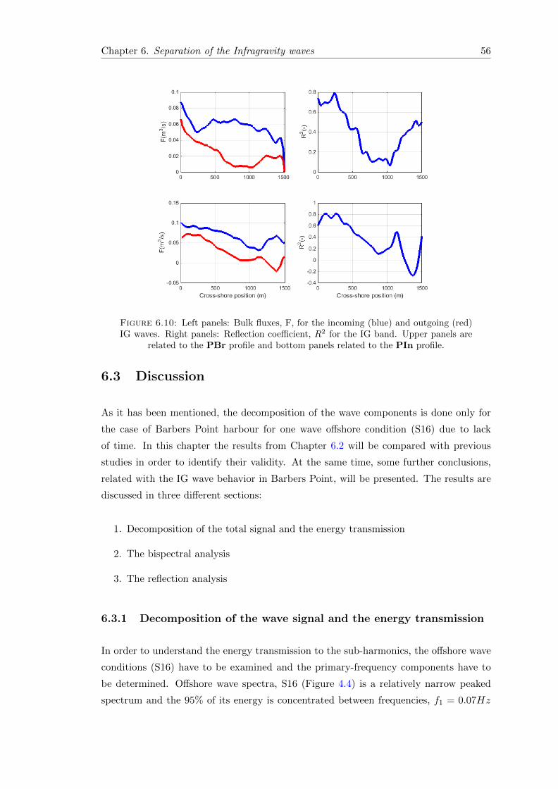
Chapter 6. Separation of the Infragravity waves 56
Figure 6.10: Left panels: Bulk fluxes, F, for the incoming (blue) and outgoing (red)IG waves. Right panels: Reflection coefficient, R2 for the IG band. Upper panels are
related to the PBr profile and bottom panels related to the PIn profile.
6.3 Discussion
As it has been mentioned, the decomposition of the wave components is done only for
the case of Barbers Point harbour for one wave offshore condition (S16) due to lack
of time. In this chapter the results from Chapter 6.2 will be compared with previous
studies in order to identify their validity. At the same time, some further conclusions,
related with the IG wave behavior in Barbers Point, will be presented. The results are
discussed in three different sections:
1. Decomposition of the total signal and the energy transmission
2. The bispectral analysis
3. The reflection analysis
6.3.1 Decomposition of the wave signal and the energy transmission
In order to understand the energy transmission to the sub-harmonics, the offshore wave
conditions (S16) have to be examined and the primary-frequency components have to
be determined. Offshore wave spectra, S16 (Figure 4.4) is a relatively narrow peaked
spectrum and the 95% of its energy is concentrated between frequencies, f1 = 0.07Hz

Chapter 6. Separation of the Infragravity waves 57
and f2 = 0.11Hz, and the major part of energy (80%) is located between f3 = 0.08Hz
and f4 = 0.10Hz. As a result, the primar sub-harmonics are expected at frequencies
fsub1 = 0.04Hz (f1 − f2) and fsub2 = 0.02Hz (f3 − f4), with the last one to be the
most empowered (originated from the interactions of the most empowered short waves).
These assumptions (about the frequency location of the sub-harmonics) can be easily
confirmed by Figure 6.6 (upper-right panel), where the short waves seem to transfer
energy to the IG waves through the frequencies, fsub1 and fsub2, at the shoaling area.
Starting from the PBr profile, the decomposition of the total signal (Chapter 6.2.1)
suggests that the IG waves start to grow after the cross-shore position, x = 700m
(Figure 6.5 and Figure 6.3), the starting point of the mild-slope zone. The IG waves
tend to start to grow at intermediate depths and this result agrees with Rijnsdorp
[2011] (and many other researchers). As it was expected, the IG energy is located close
to the subharmonic, fsub2 = 0.02Hz (Figure 6.3), at the starting point. Moving shore-
wards, energy seems to be transmitted to other sub-harmonics due to non-linear wave
interactions. The results for the spectral evolution (Figure 6.3) is somewhat similar to
the patterns that Michallet et al. [2014] described (Figure 2.1).
With regard to the PIn profile, IG waves are starting to grow, after the cross-shore
position, x = 1100m, inside the entrance channel zone (Figure 6.4). For this profile,
the IG waves originate from areas outside of this profile. At first, the IG waves start to
grow after a significant reduce of the short wave energy (Figure 6.4), in deeper waters
than to the PBr profile. Additionally, the IG wave energy seems to be concentrated in
several frequency components, at the starting point, x = 1100m. The reduced boundness
of the IG waves is caused by reflections (edge and leaky waves) due to the shore and
the vertical structures. More about this behavior will be explained in Chapter 6.3.3.
Finally, Figure 6.5 shows that the Barbers Point harbour is well protected by the short
waves, but not from the IG waves. The IG waves (as long waves) seem to be strongly
affected by refraction due to the north edges (Figure 6.1) of the channel, leading to IG
propagation into the harbour. On the other hand, short waves (weakly refracted) are
following another path to the adjacent shore.
6.3.2 Bispectral analysis
The bispectral analysis (Figure 6.6, upper-right panel) agrees with Henderson et al.
[2006], that swell frequencies (0.08 − 0.11Hz) transmit energy to their sub-harmonics
(fsub1 = 0.4Hz and fsub2 = 0.2). Within the breaking zone , the IG waves start to
release due to short wave energy dissipation. As Eldeberky [1996] stated, the IG waves
with the lowest frequency are expected to be released first ((Figure 6.6, bottom-left
Chapter 6. Separation of the Infragravity waves 58
panel) and the high (in terms of frequency) IG waves are following . Finally, in the
swash-zone, a major part of IG waves is released and slight increase of bicoherence is
dictating re-generation of bound IG waves in that area (consistent with [Michallet et al.,
2014] research).
Bicoherenece and biphase for the PBr profile shows similar trend to Ruessink [1998],El-
deberky [1996] (Figure 3.2) and Sheremet et al. [2002]. The IG wave is loosely bounded
with the short waves, between x = 0m and x = 1100m (Figure 6.8, upper panel).
Reduced coupling (bicoherence) is caused by the leaky IG waves as Eldeberky [1996]
presented. Between x = 1100m and x = 1200m , short wave- IG wave interactions
are amplified as the wave approaches the breaking zone. Inside the breaking zone the
complexity of the interpretation increases. The short waves start to break, starting from
the short wave components with the highest amount of energy. If the breaking points,
for each short wave component, were located at the same position, a sharp decrease of
bicoherence would be expected at the breaking point (due to the total release of the IG
waves). However, the bicoherence drops significantly (0.7 to 0.4) between x = 1250m
and x = 1300m, remains constant for 40m and decreases again, reaching bicoherence of
b = 0.3 at x = 1400m. The coupling between IG and short waves starts again after the
x = 1400m (surf-zone). The simulated behavior of IG waves inside the breaking and
the surf zone agrees with the observations of Michallet et al. [2014] and Guedes et al.
[2013].
For the PIn profile, the interpretation of the IG wave behaviour is relatively simple
due to the absence of breaking phenomena (in the transect PIn) . Between x = 0m
and x = 900m, there are no severe fluctuations and bicoherence is similar to the PBr
profile for this area. However, there is a significant reduction of bicoherence between
x = 1000m and x = 1250m, and after this zone, bicoherence increases again to b = 0.34
until the inlet. The adjacent shore is considered as the origin of the free IG waves at
the zone x = 1000 − 1250. Another reason of that reduction is the release of IG waves
due to refraction, which is explained in Chapter 6.3.1 (last paragraph).
6.3.3 The reflection analysis
Starting from the PBr profile (Figure 6.10, upper right panel), IG waves experience
a significant reflection (R2= 0.2-0.8), but they are not fully reflected (R2=1). This
means that there is energy dissipation of IG waves due to several mechanisms (Chap-
ter 2.4). However, the reduction of the reflection coefficient in the surf zone is not severe
[de Bakker et al., 2013] and no IG breaking phenomena are expected. The dominant
dissipation mechanism is probably the interaction of the incoming short waves with
Chapter 6. Separation of the Infragravity waves 59
the outgoing IG waves, as Thomson et al. [2006] identified (Chapter 2.4). IG energy
fluxes for the incoming waves drop significantly compared to those for the out-coming
waves, which are remaining relatively constant. The results for the reflection analysis
are consistent with the research of Sheremet et al. [2002] and de Bakker et al. [2013]
(Figure 2.8).
For the PIn profile (Figure 6.10, bottom right panel), the interpretation of the fluxes
variations is more complex due to the effect of the adjacent areas and the basin. As
mentioned in Chapter 6.3.2, there are evidences that reflected IG waves (from the adja-
cent areas) are affecting the entrance channel of the Barbers Point harbour, especially
between x = 1000 − 1400. Edge waves, generated at the shore, are trapped inside the
surf-zone and enter to the entrance channel, causing the peak of the reflection coefficient
at the location x = 1200. Continuing closer to the inlet, the energy of the reflected
waves is reduced due to the effect of the harbour. IG waves are reflected from the
vertical structures of the basin, but they remain inside the harbour.

Chapter 7
Conclusion
As clarified in Chapter 1, the scope of this thesis is to provide an insight to the IG
behavior close harbours. The harbour of Barbers Point in Hawaii has been chosen as
a case study. This thesis constitutes one of the first extensive researches related to the
simulation and analysis of IG waves in a two-dimensional domain. Here, the answers to
the research questions of Chapter 1.4 are summarized and some recommendations for
future studies are presented.
7.1 Answering the research questions
In general, IG waves are generated by the interactions of the short waves. Short wave
frequency components tend to interact with each other and transmit energy to sub and
super harmonics. This energy transmission is amplified as the waves propagates shore-
wards and the effects of the bottom becomes dominant. IG waves are the generated sub-
harmonics with frequency between 0.005- 0.05 Hz and they are propagating bounded to
the short waves (Res. question 1a). After high energy-fluctuations to the short waves,
IG waves are released and they propagate freely. Energy variations could occur due
to breaking phenomena or reflection (Res. question 1b). After their release, IG waves
dissipate because of their interactions with the short waves, IG wave breaking at low-
depths or bottom friction. Both free and bound IG waves could induce resonance to the
basin, excessive oscillations to the moored vessels and sediment transport close to the
harbour inlet (Res. question 1c).
According to literature, there are several types of numerical tools for the IG wave sim-
ulation and they can be discretized by their fundamental equations. RANS (Reynolds
Averaged Navier Stokes) models are too computational expensive for two-dimensional
60

Chapter 7. Conclusion and recommendations 61
cases. On the other hand, Boussinesq models are widely used but they are inaccurate
for large depths (for the case of Barbers Point harbour the offshore boundary depth is
50 m). NSWE (Non-linear Shallow Water Equations) models are not so computational
intense compared to other type of models. However, due to their equations, NSWE
models are incapable of simulating waves at large depths (shallow water equations) and
thus calculating the evolution of IG waves (due to the depth integrated shallow water
equations (Res. question 2a+2b). SWASH [Zijlema et al., 2011] (NSWE model) over-
comes these restrictions. The option of vertical layer separation is implemented to the
model (SWASH), making the shallow-water equations accurate even for large depths.
Additionally, a non-hydrostatic term is added to the momentum equations, leading to
the reintroduction of the vertical flow motion. The product of this phase-resolving model
is the surface elevation series and the flow velocities series, along and cross-shore (Res.
question 2d). In order to proceed to the IG wave investigation a post-data analysis
is needed. FFT (Chapter 3.2) method is used to separate the total wave for different
frequency components and then bispectral analysis determines the correlation between
these frequency components (Res. question 2c).
Continuing with the set-up of the model, the proper simulation time, for the case of
Barbers Point harbour, is considered 75-80 mins. There is a need of 10 mins to arise an
equilibrium (for a bi-chromatic case) and approximately 70 mins to achieve a statistically
accurate IG wave calculation (simulate more than 100 IG waves) (Res. question 3a).
The computational grid is assumed as 3 x 7m, in order to efficiently simulate the short
(generation force of IG waves) and the IG waves (Res. question 3b). Off-shore boundary
is considered as weakly-reflective, letting the shore reflected waves to escape the domain.
However, the same option is not available for the lateral boundaries and sponge layers
are used in order to gradually dump the waves at these areas. The reasonable width of
200 m sponge layers is chosen to absorb the energy of the waves (both short and IG) at
the lateral boundaries (Res. question 3c). Finally, the vertical structures are considered
fully reflective for this thesis project. This assumption leads to inaccuracies to the short
wave simulation inside the basin, but it works efficiently for the IG waves (Scope of the
thesis) due to the large IG wave length (Res. question 3d).
The model seems to be highly-sensitive to the width of the sponge layers and the grid
resolution. For small widths of sponge layers, the reflected waves cause overestimation of
the IG wave height. Additionally, a coarse grid resolution leads to the same magnitude
(same as the sponge layers) of IG height overestimation (Res. question 3e). As it was
expected, the NSWE model, SWASH, is inaccurate for large depths of the offshore region
and the use of two vertical layers is suggested. In addition, the NSWE model is slightly
sensitive to the location of the breaking zone (defined by the breaking parameter),
proving that breaking phenomena have a major effect on the release and not on the
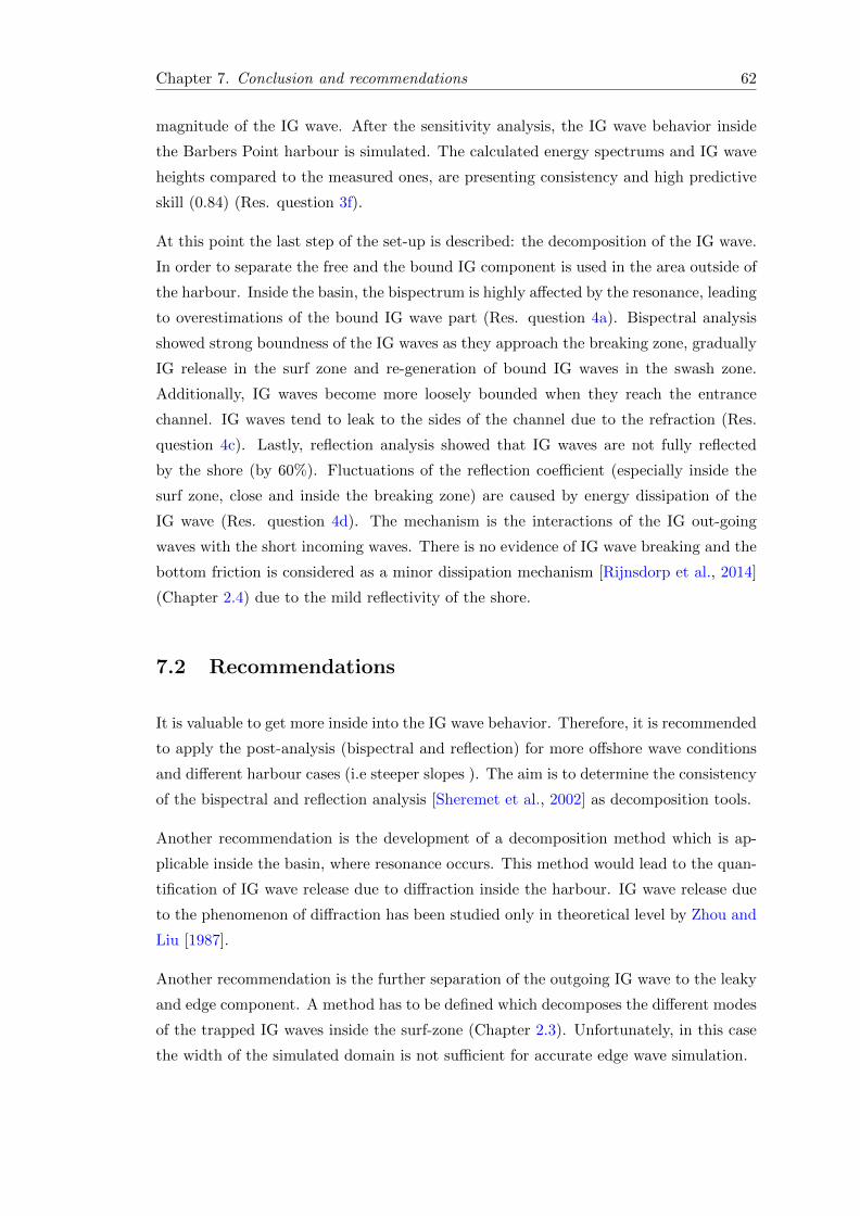
Chapter 7. Conclusion and recommendations 62
magnitude of the IG wave. After the sensitivity analysis, the IG wave behavior inside
the Barbers Point harbour is simulated. The calculated energy spectrums and IG wave
heights compared to the measured ones, are presenting consistency and high predictive
skill (0.84) (Res. question 3f).
At this point the last step of the set-up is described: the decomposition of the IG wave.
In order to separate the free and the bound IG component is used in the area outside of
the harbour. Inside the basin, the bispectrum is highly affected by the resonance, leading
to overestimations of the bound IG wave part (Res. question 4a). Bispectral analysis
showed strong boundness of the IG waves as they approach the breaking zone, gradually
IG release in the surf zone and re-generation of bound IG waves in the swash zone.
Additionally, IG waves become more loosely bounded when they reach the entrance
channel. IG waves tend to leak to the sides of the channel due to the refraction (Res.
question 4c). Lastly, reflection analysis showed that IG waves are not fully reflected
by the shore (by 60%). Fluctuations of the reflection coefficient (especially inside the
surf zone, close and inside the breaking zone) are caused by energy dissipation of the
IG wave (Res. question 4d). The mechanism is the interactions of the IG out-going
waves with the short incoming waves. There is no evidence of IG wave breaking and the
bottom friction is considered as a minor dissipation mechanism [Rijnsdorp et al., 2014]
(Chapter 2.4) due to the mild reflectivity of the shore.
7.2 Recommendations
It is valuable to get more inside into the IG wave behavior. Therefore, it is recommended
to apply the post-analysis (bispectral and reflection) for more offshore wave conditions
and different harbour cases (i.e steeper slopes ). The aim is to determine the consistency
of the bispectral and reflection analysis [Sheremet et al., 2002] as decomposition tools.
Another recommendation is the development of a decomposition method which is ap-
plicable inside the basin, where resonance occurs. This method would lead to the quan-
tification of IG wave release due to diffraction inside the harbour. IG wave release due
to the phenomenon of diffraction has been studied only in theoretical level by Zhou and
Liu [1987].
Another recommendation is the further separation of the outgoing IG wave to the leaky
and edge component. A method has to be defined which decomposes the different modes
of the trapped IG waves inside the surf-zone (Chapter 2.3). Unfortunately, in this case
the width of the simulated domain is not sufficient for accurate edge wave simulation.

Chapter 7. Conclusion and recommendations 63
From an engineering point of view, the identification of IG wave mitigation measures
is interesting. There are no direct measures to avoid the presence of IG waves inside
the basin due to their large wave-length. However, adjustments to the bathymetry
(especially of the entrance channel) would affect the refraction of the longer components,
relocating the propagation direction of the IG waves at the adjacent shores. Additionally,
the breakwaters inside the surf-zone and parallel to the shoreline would lead to the
relocation of the edge waves [Chen et al., 2004a].
With regard to the numerical model,SWASH, a better representation of the boundaries
is suggested. Spatial variation of the wave conditions at the offshore boundaries would
lead to more accurate simulations. Additionally, the option of weakly reflective lateral
boundaries would avoid the existence of reflective waves (on the lateral boundaries)
inside the domain. Finally, the vertical discretization of the porosity would be helpful
for a better representation of the harbour structures.
Appendix A
Background knowledge
A.1 Hilbert transformation
The boundness of the IG wave is related to the variation of the wave amplitude. In
general, the wave envelope quantifies these amplitude fluctuations. Hilbert transforma-
tion is applied in order to obtain the wave envelope for the short waves. The short
wave surface elevation signal is decomposed by the total (by using FFT method) and
the Hilbert transformation function of MATLAB is used on that signal. Continuing, the
frequency limits of the wave envelope have to correspond with the IG wave frequency
limits (0.005-0.05Hz) for this thesis project. The wave envelope is calculated by using
Eq. A.1 [Janssen et al., 2003]:
|α(t)| = |ζsw(t) + iγsw(t)|IG (A.1)
where t is the time, γ is the Hibert operator, ζsw the surface elevation for the short
waves and α the envelope of the surface elevation. Finally, IG superscript denotes the
IG frequency restrictions.
A.2 Cross-correlation
Cross-Correlation (also called cross-covariance) between two input signals is a kind of
template matching. Cross-correlation can be done in any number of dimensions. The
one-dimensional normalized cross-correlation between two input signals is defined as:
64

Appendix A. Hilbert transformation 65
r(d) =
∑((x(i)−mx) ∗ (y(i− d)−my))√∑(x(i)−mx)2
√∑(y(i− d)−my)2
(A.2)
The coefficient,r, is a measurement of the size and direction of the linear relationship
between variables x and y (d is the time lag and mx and my are the mean values of the
x and y series respectively). If these variables move together, where they both rise at an
identical rate, then r= +1. If the other variable does not budge, then r= 0. If the other
variable falls at an identical rate, then r= -1. If r is greater than zero, we have positive
correlation. If r is less than zero, we have negative correlation.
A.3 Breaking criterion
Weggel [1972] developed an equation for the breaker depth index from previous labora-
tory data collected on slopes of 1/5,1/10,1/15,1/20, and1/50.The resulting relationship
is expressed as:
Hb
db= bm − am
Hb
gT 2(A.3)
where T is the wave period, Hb is the significant height at the breaking point and db
the depth when breaking occurs. The parameters am and bm are empirically determined
functions of beach slope (m), given by:
am = 43.8(1− e19m) (A.4)
bm =1.56
1 + e−19.5m(A.5)

Appendix B
Sensitivity analysis and results
for the S17 storm
Figure B.1: The IG wave energy spectrum for S17 and for different values of direc-tional spreading at the location 059-P1. Blue is the measured form CDIP, green forms=10, red for ms=15, cyan for ms=20, magenta for ms=25 and yellow for ms=40.
66
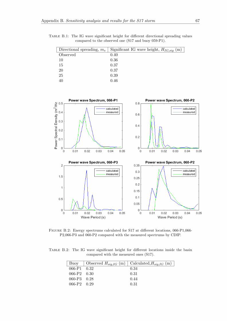
Appendix B. Sensitivity analysis and results for the S17 storm 67
Table B.1: The IG wave significant height for different directional spreading valuescompared to the observed one (S17 and buoy 059-P1).
Directional spreading, ms Significant IG wave height, HIG,sig (m)
Observed 0.4010 0.3615 0.3720 0.3725 0.3940 0.46
Figure B.2: Energy spectrums calculated for S17 at different locations, 066-P1,066-P2,066-P3 and 060-P2 compared with the measured spectrums by CDIP.
Table B.2: The IG wave significant height for different locations inside the basincompared with the measured ones (S17).
Buoy Observed Hsig,IG (m) Calculated,Hsig,IG (m)
066-P1 0.32 0.34066-P2 0.30 0.31060-P3 0.28 0.44066-P2 0.29 0.31

Appendix C
Amplification factors for the
Barbers Point harbour
The amplification factor is the ratio between the energy at several gauges inside the basin
and the energy outside of the basin and close to the inlet. Outside of the Barbers Point
harbour, at the buoy 059-P1, the IG waves are considered fully developed. Amplification
of the low-frequency energy inside the basin is considered as an effect of the resonance.
So, low-frequency components with amplification factor higher than 1 are considered as
one of the basin;’s natural frequency.
68

Appendix C. Amplification factors for the Barbers Point harbour 69
Figure C.1: Amplification factor for different locations inside the basin (066-P1,066-P2,066-P3 and 060-P2) for the S16.

Appendix C. Amplification factors for the Barbers Point harbour 70
Figure C.2: Amplification factor for different locations inside the basin (066-P1,066-P2,066-P3 and 060-P2) for the S17.
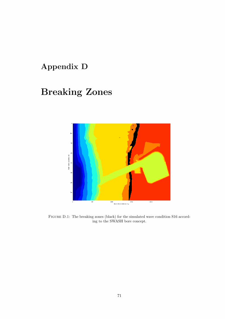
Appendix D
Breaking Zones
Figure D.1: The breaking zones (black) for the simulated wave condition S16 accord-ing to the SWASH bore concept.
71

Appendix D. Breaking Zones 72
Figure D.2: The breaking zones (black) for the simulated wave condition S16 accord-ing to the Weggel [1972] breaking criterion.

Appendix E
Directional spectra
The directional spectrums are calculated by using MATLAB. The surface elevation, ζ,
and the velocities alongshore (uy) and cross-shore (ux) are used in order to calculate the
energy magnitude and the propagation direction of the wave. Waves are separated to IG
and short waves and the directional spectrums for different locations (both profiles, PBr
and PIn) are presented. Finally, the offshore boundary is located at the 90o degrees
and the Barbers point harbor at the 270o degrees.
Figure E.1: Directional spectrum for the short waves at the location, x = 200m(Profile PBr).
73
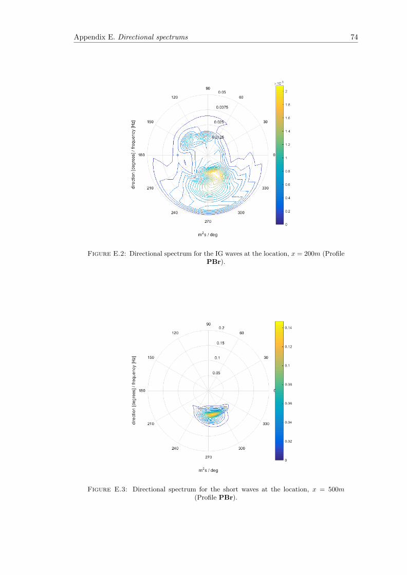
Appendix E. Directional spectrums 74
Figure E.2: Directional spectrum for the IG waves at the location, x = 200m (ProfilePBr).
Figure E.3: Directional spectrum for the short waves at the location, x = 500m(Profile PBr).

Appendix E. Directional spectrums 75
Figure E.4: Directional spectrum for the IG waves at the location, x = 500m (ProfilePBr).
Figure E.5: Directional spectrum for the short waves at the location, x = 1200m(Profile PBr).
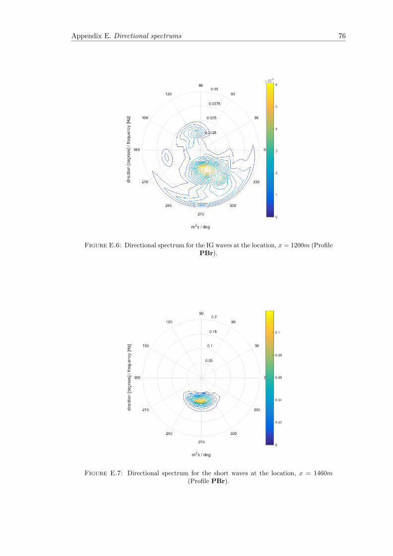
Appendix E. Directional spectrums 76
Figure E.6: Directional spectrum for the IG waves at the location, x = 1200m (ProfilePBr).
Figure E.7: Directional spectrum for the short waves at the location, x = 1460m(Profile PBr).

Appendix E. Directional spectrums 77
Figure E.8: Directional spectrum for the IG waves at the location, x = 1460m (ProfilePBr).
Figure E.9: Directional spectrum for the short waves at the location, x = 200m(Profile PIn).
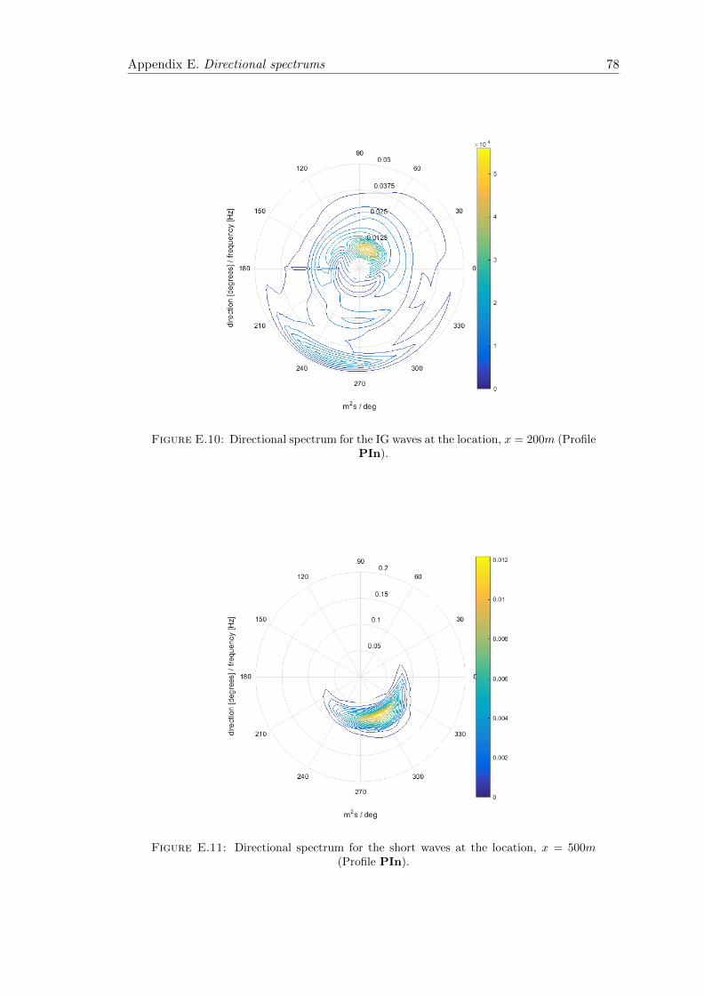
Appendix E. Directional spectrums 78
Figure E.10: Directional spectrum for the IG waves at the location, x = 200m (ProfilePIn).
Figure E.11: Directional spectrum for the short waves at the location, x = 500m(Profile PIn).

Appendix E. Directional spectrums 79
Figure E.12: Directional spectrum for the IG waves at the location, x = 500m (ProfilePIn).
Figure E.13: Directional spectrum for the short waves at the location, x = 1200m(Profile PIn).

Appendix E. Directional spectrums 80
Figure E.14: Directional spectrum for the IG waves at the location, x = 1200m(Profile PIn).
Figure E.15: Directional spectrum for the short waves at the location, x = 1460m(Profile PIn).
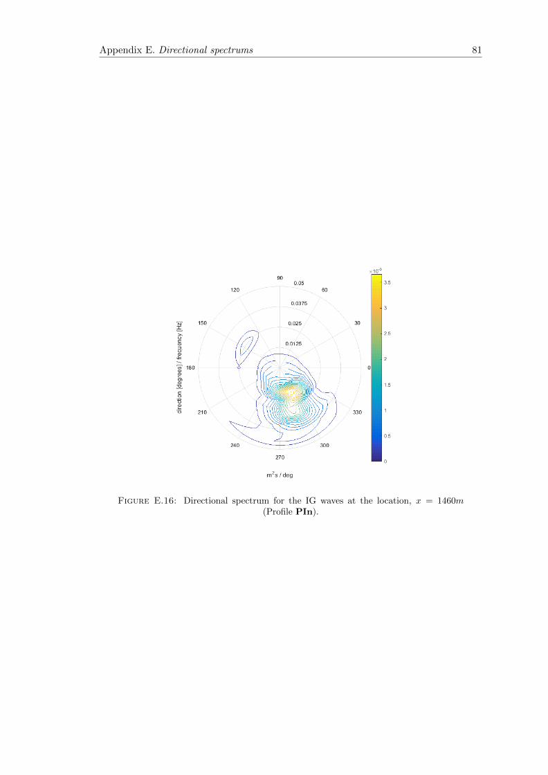
Appendix E. Directional spectrums 81
Figure E.16: Directional spectrum for the IG waves at the location, x = 1460m(Profile PIn).

Appendix F
Bispectra analysis for the PIn
profile
Figure F.1: Normalized bispectrum (bicoherence) at the location x = 200m for thePIn profile.
82

Appendix E. Bispectra analysis for the PIn profile 83
Figure F.2: Normalized bispectrum (bicoherence) at the location x = 500m for thePIn profile.
Figure F.3: Normalized bispectrum (bicoherence) at the location x = 1200m for thePIn profile.

Appendix E. Bispectra analysis for the PIn profile 84
Figure F.4: Normalized bispectrum (bicoherence) at the location x = 1460m for thePIn profile.

Bibliography
A Sheremet, RT Guza, Steve Elgar, and THC Herbers. Observations of nearshore in-
fragravity waves: Seaward and shoreward propagating components. Journal of Geo-
physical Research: Oceans (1978–2012), 107(C8):10–1, 2002.
Walter Munk. Origin and generation of waves. Coastal Engineering Proceedings, 1(1),
1950. ISSN 2156-1028. URL https://icce-ojs-tamu.tdl.org/icce/index.php/
icce/article/view/904.
Herve Michallet, Gerben Ruessink, Mariana VL Rocha, Anouk De Bakker, Dominic Van
Der A, Andrea Ruju, Paulo A Silva, Nadia Senechal, Vincent Marieu, Marion Tissier,
et al. Globex: Wave dynamics on a shallow sloping beach. In HYDRALAB IV Joint
User Meeting, Lisbon, July 2014, 2014.
THC Herbers, Steve Elgar, RT Guza, and WC O’Reilly. Infragravity-frequency (0.005-
0.05 hz) motions on the shelf. part ii: Free waves. Journal of physical oceanography,
25(6):1063–1079, 1995.
Michael S Longuet-Higgins and R W Stewart. Radiation stress and mass transport in
gravity waves, with application to ‘surf beats’. Journal of Fluid Mechanics, 13(04):
481–504, 1962.
JA Battjes, HJ Bakkenes, TT Janssen, and AR Van Dongeren. Shoaling of subharmonic
gravity waves. Journal of Geophysical Research: Oceans (1978–2012), 109(C2), 2004.
Peter J McComb, David L Johnson, and Brett J Beamsley. Numerical study of options
to reduce swell and long wave penetration at port geraldton. Coasts and Ports 2009:
In a Dynamic Environment, page 490, 2009.
KT Holland and Robert A Holman. Wavenumber-frequency structure of infragrav-
ity swash motions. Journal of Geophysical Research: Oceans (1978–2012), 104(C6):
13479–13488, 1999.
IK Van Giffen. Long wave case study for barbers point harbour, hawaii. 2003.
85

Bibliography 86
Anouk de Bakker, Marion Tissier, Vincent Marieu, Nadia Senechal, Andrea Ruju, Javier
Lara, and BG Ruessink. Infragravity wave propagation and dissipation on a low-
sloping laboratory beach. In Proceedings of the Conference on Coastal Dynamics,
2013.
Yasser Eldeberky. Nonlinear transformation of wave spectra in the nearshore. TU Delft,
Delft University of Technology, 1996.
Mark Buckley, Ryan Lowe, and Jeff Hansen. Evaluation of nearshore wave models in
steep reef environments. Ocean Dynamics, 64(6):847–862, 2014.
Richard J Weggel. Maximum breaker height. ” Journal of the Waterways, Harbors and
Coastal Engineering Division, 98(4):529–548, 1972.
THC Herbers and MC Burton. Nonlinear shoaling of directionally spread waves on a
beach. Journal of Geophysical Research: Oceans (1978–2012), 102(C9):21101–21114,
1997.
Spahr C Webb, Xin Zhang, and Wayne Crawford. Infragravity waves in the deep ocean.
Journal of Geophysical Research: Oceans (1978–2012), 96(C2):2723–2736, 1991.
RT Guza and Edward B Thornton. Observations of surf beat. Journal of Geophysical
Research: Oceans (1978–2012), 90(C2):3161–3172, 1985.
Guan-Yu Chen, Chung-Ching Chien, Ching-Ho Su, and Hsiang-Mao Tseng. Resonance
induced by edge waves in hua-lien harbor. Journal of oceanography, 60(6):1035–1043,
2004a.
Wim Van Der Molen, Patricio Monardez, and Ap Van Dongeren. Numerical simulation
of long-period waves and ship motions in tomakomai port, japan. Coastal Engineering
Journal, 48(01):59–79, 2006.
Reginald A Beach and Richard W Sternberg. Suspended sediment transport in the surf
zone: response to cross-shore infragravity motion. Marine Geology, 80(1):61–79, 1988.
Vincent Leys and Ryan P Mulligan. Modelling coastal sediment transport for
harbour planning: selected case studies. Sediment Transport, http://www.
intechopen. com/articles/show/title/modelling-coastal-sediment-transport-forharbour-
planning-selected-case-studies, 2011.
Okey Nwogu and Zeki Demirbilek. Infragravity wave motions and runup over shallow
fringing reefs. Journal of waterway, port, coastal, and ocean engineering, 136(6):295–
305, 2010.

Bibliography 87
Marcel Zijlema, Guus Stelling, and Pieter Smit. Swash: An operational public domain
code for simulating wave fields and rapidly varied flows in coastal waters. Coastal
Engineering, 58(10):992–1012, 2011.
Dano Roelvink, Ad Reniers, AP van Dongeren, Jaap van Thiel de Vries, Robert McCall,
and Jamie Lescinski. Modelling storm impacts on beaches, dunes and barrier islands.
Coastal Engineering, 56(11):1133–1152, 2009.
Dirk Pieter Rijnsdorp, Pieter Bart Smit, and Marcel Zijlema. Non-hydrostatic modelling
of infragravity waves using swash. Coastal Engineering Proceedings, 1(33):currents–27,
2012.
Costas Emmanuel Synolakis. Green’s law and the evolution of solitary waves. Physics
of Fluids A: Fluid Dynamics (1989-1993), 3(3):490–491, 1991.
Eizo Nakaza and Mikio Hino. Bore-like surf beat in a reef zone caused by wave groups
of incident short period waves. Fluid Dynamics Research, 7(2):89, 1991.
Graham Symonds, David A Huntley, and Anthony J Bowen. Two-dimensional surf beat:
Long wave generation by a time-varying breakpoint. Journal of Geophysical Research:
Oceans (1978–2012), 87(C1):492–498, 1982.
Guohai Dong, Xiaozhou Ma, Jianwu Xu, Yuxiang Ma, and Gang Wang. Experimental
study of the transformation of bound long waves over a mild slope with ambient
currents. Coastal Engineering, 56(10):1035–1042, 2009.
CHINPU Zhou and PHILIP L-F Liu. Second-order low-frequency wave forces on a
vertical circular cylinder. Journal of Fluid Mechanics, 175:143–156, 1987.
MW McBride, JV Smallman, and NWH Allsop. Guidelines for the hydraulic design of
harbour entrances. 1996.
Gordon S Harkins and Michael J Briggs. Resonant forcing of harbors by infragravity
waves. Coastal Engineering Proceedings, 1(24), 1994.
F Ursell. Edge waves on a sloping beach. Proceedings of the royal society of London.
Series A. Mathematical and Physical Sciences, 214(1116):79–97, 1952.
EC Bowers. Harbour resonance due to set-down beneath wave groups. Journal of Fluid
Mechanics, 79(01):71–92, 1977.
Y Ciriano, A Falques, and MA Losada. Resonance of a harbour under edge waves
forcing. In Coastal Engineering 2000, pages 3580–3591. ASCE, 2001.
Bibliography 88
Guan-Yu Chen, Chung-Ching Chien, Ching-Ho Su, and Hsiang-Mao Tseng. Resonance
induced by edge waves in hua-lien harbor. Journal of oceanography, 60(6):1035–1043,
2004b.
Jim Thomson, Steve Elgar, Britt Raubenheimer, THC Herbers, and RT Guza. Tidal
modulation of infragravity waves via nonlinear energy losses in the surfzone. Geophys-
ical Research Letters, 33(5), 2006.
A Van Dongeren, J Battjes, T Janssen, J Van Noorloos, K Steenhauer, G Steenber-
gen, and AJHM Reniers. Shoaling and shoreline dissipation of low-frequency waves.
Journal of Geophysical Research: Oceans (1978–2012), 112(C2), 2007.
Stephen M Henderson and AJ Bowen. Observations of surf beat forcing and dissipation.
Journal of Geophysical Research: Oceans (1978–2012), 107(C11):14–1, 2002.
Stephen M Henderson, RT Guza, Steve Elgar, THC Herbers, and AJ Bowen. Nonlinear
generation and loss of infragravity wave energy. Journal of Geophysical Research:
Oceans (1978–2012), 111(C12), 2006.
Dirk P Rijnsdorp, Pieter B Smit, and Marcel Zijlema. Non-hydrostatic modelling of
infragravity waves under laboratory conditions. Coastal Engineering, 85:30–42, 2014.
Jaak Monbaliu, Roberto Padilla-Hernandez, Julia C Hargreaves, Juan Carlos Carretero
Albiach, Weimin Luo, Mauro Sclavo, and Heinz Guenther. The spectral wave model,
wam, adapted for applications with high spatial resolution. Coastal engineering, 41
(1):41–62, 2000.
Philippe Bonneton, Florent Chazel, David Lannes, Fabien Marche, and Marion Tissier.
A splitting approach for the fully nonlinear and weakly dispersive green–naghdi model.
Journal of Computational Physics, 230(4):1479–1498, 2011.
Mara Tonelli and Marco Petti. Shock-capturing boussinesq model for irregular wave
propagation. Coastal Engineering, 61:8–19, 2012.
M Tissier, P Bonneton, F Marche, F Chazel, and D Lannes. A new approach to handle
wave breaking in fully non-linear boussinesq models. Coastal Engineering, 67:54–66,
2012.
Per A Madsen, OR Sørensen, and HA Schaffer. Surf zone dynamics simulated by a
boussinesq type model. part ii: Surf beat and swash oscillations for wave groups and
irregular waves. Coastal Engineering, 32(4):289–319, 1997.
Pieter Smit, Marcel Zijlema, and Guus Stelling. Depth-induced wave breaking in a
non-hydrostatic, near-shore wave model. Coastal Engineering, 76:1–16, 2013.

Bibliography 89
Gangfeng Ma, Fengyan Shi, and James T Kirby. Shock-capturing non-hydrostatic model
for fully dispersive surface wave processes. Ocean Modelling, 43:22–35, 2012.
JL Lara, IJ Losada, and R Guanche. Wave interaction with low-mound breakwaters
using a rans model. Ocean engineering, 35(13):1388–1400, 2008.
Tomohiro Suzuki, Toon Verwaest, William Veale, Koen Trouw, and Marcel Zijlema. A
numerical study on the effect of beach nourishment on wave overtopping in shallow
foreshores. Coastal Engineering Proceedings, 1(33):waves–50, 2012.
Changhoon Lee, Woo Sun Park, Yong-Sik Cho, and Kyung Doug Suh. Hyperbolic
mild-slope equations extended to account for rapidly varying topography. Coastal
Engineering, 34(3):243–257, 1998.
G Stelling and M Zijlema. An accurate and efficient finite-difference algorithm for
non-hydrostatic free-surface flow with application to wave propagation. International
Journal for Numerical Methods in Fluids, 43(1):1–23, 2003.
DCL Lam and RB Simpson. Centered differencing and the box scheme for diffusion
convection problems. Journal of Computational Physics, 22(4):486–500, 1976.
Eric Blayo and Laurent Debreu. Revisiting open boundary conditions from the point of
view of characteristic variables. Ocean modelling, 9(3):231–252, 2005.
JK Kostense. Measurements of surf beat and set-down beneath wave groups. Coastal
Engineering Proceedings, 1(19), 1984.
Yuxiang Ma, Guohai Dong, and Xiaozhou Ma. Separation of low-frequency waves by an
analytical method. Coastal Engineering Proceedings, 1(32):waves–64, 2011.
Klaus Hasselmann, Walter Munk, and Gordon MacDonald. Bispectra of ocean waves.
Time Series Analysis, pages 125–139, 1963.
BG Ruessink. Bound and free infragravity waves in the nearshore zone under breaking
and nonbreaking conditions. Journal of Geophysical Research: Oceans (1978–2012),
103(C6):12795–12805, 1998.
GuoHai Dong, Gang Wang, XiaoZhou Ma, and YuXiang Ma. Numerical study of tran-
sient nonlinear harbor resonance. Science China Technological Sciences, 53(2):558–
565, 2010.
Young C Kim and Edward J Powers. Digital bispectral analysis and its applications to
nonlinear wave interactions. Plasma Science, IEEE Transactions on, 7(2):120–131,
1979.

Bibliography 90
Thomas J Maccarone. The biphase explained: understanding the asymmetries in cou-
pled fourier components of astronomical time series. Monthly Notices of the Royal
Astronomical Society, page stt1546, 2013.
JOAN Alabart, AGUSTIN Sanchez-Arcilla, and G Ph Van Vledder. Analysis of the
performance of swash in harbour domains. In Proceedings of the 3rd IAHR Europe
congress, 1-10.(2014), Porto, Portugal. IHAR, 2014.
Arnold Verruijt et al. Theory of groundwater flow. 1970.
Bart Mellink. Numerical and experimental research of wave interaction with a porous
breakwater. 2012.
Swash team, 2015. User Manual SWASH version 2.00. URL http://swash.
sourceforge.net/download/zip/swashuse.pdf.
EC Bowers. Low frequency waves in intermediate water depths. Coastal Engineering
Proceedings, 1(23), 1992.
AJHM Reniers, AR Van Dongeren, JA Battjes, and EB Thornton. Linear modeling of
infragravity waves during delilah. Journal of Geophysical Research: Oceans (1978–
2012), 107(C10):1–1, 2002.
AJHM Reniers, MJ Groenewegen, KC Ewans, S Masterton, GS Stelling, and J Meek.
Estimation of infragravity waves at intermediate water depth. Coastal Engineering,
57(1):52–61, 2010.
DP Rijnsdorp. Numerical modelling of infragravity waves in coastal regions. PhD thesis,
TU Delft, Delft University of Technology, 2011.
Rafael Guedes, Karin R Bryan, and Giovanni Coco. Observations of wave energy fluxes
and swash motions on a low-sloping, dissipative beach. Journal of Geophysical Re-
search: Oceans, 118(7):3651–3669, 2013.
TT Janssen, JA Battjes, and AR Van Dongeren. Long waves induced by short-wave
groups over a sloping bottom. Journal of Geophysical Research: Oceans (1978–2012),
108(C8), 2003.
Top Related