


Languages
Pages
Legal


MD 021 - Management and Operations
Inventory Management
Introduction
Economic Order Quantity (EOQ) Model
Economic Production Quantity Model
Quantity Discounts Model
Reorder Point (Q System)
Shortages and Service Levels
Single Period Model
1
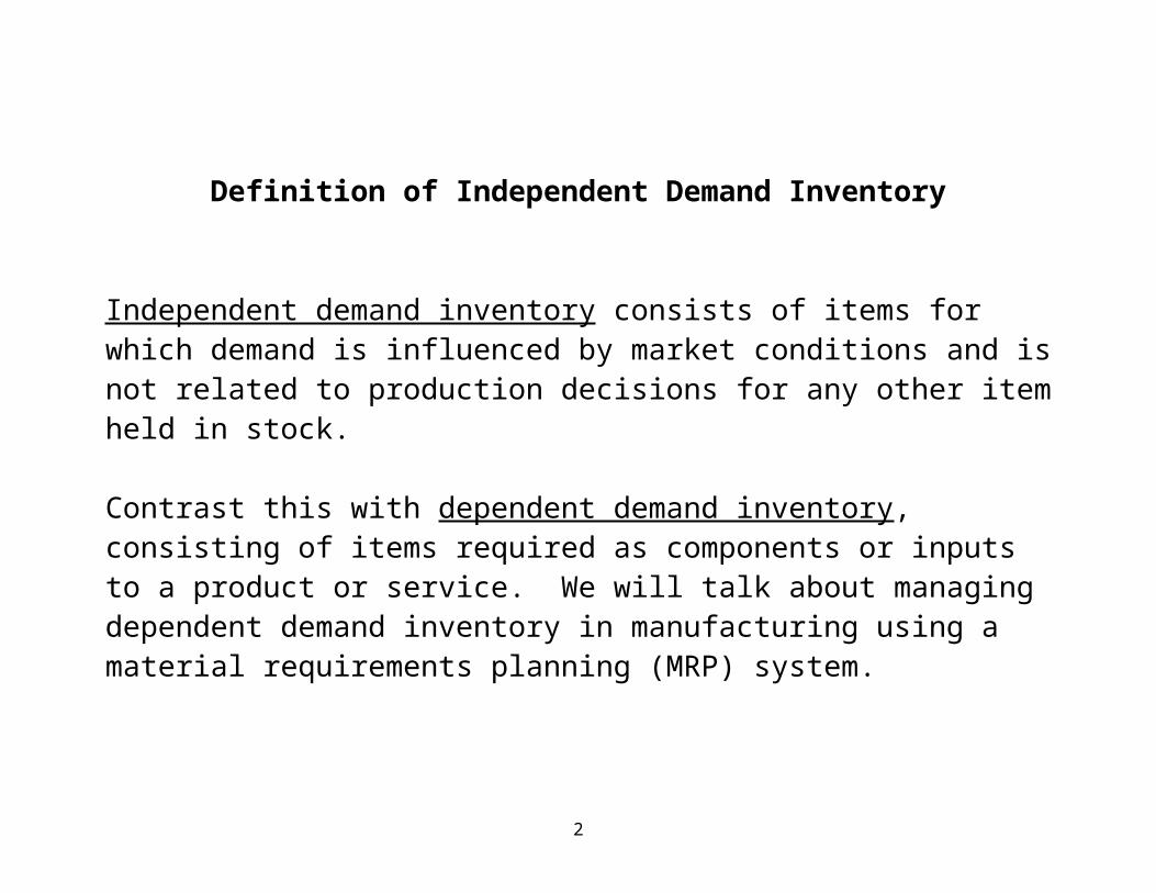
Definition of Independent Demand Inventory
Independent demand inventory consists of items for which demand is influenced by market conditions and is not related to production decisions for any other item held in stock.
Contrast this with dependent demand inventory, consisting of items required as components or inputs to a product or service. We will talk about managing dependent demand inventory in manufacturing using a material requirements planning (MRP) system.
2

Types of Inventory
Cycle inventory
Safety stock
Anticipation inventory
Pipeline inventory
3

Managing Independent Demand Inventory
Managing independent demand inventory involves answering two questions:
How much to order?
When to order?
4
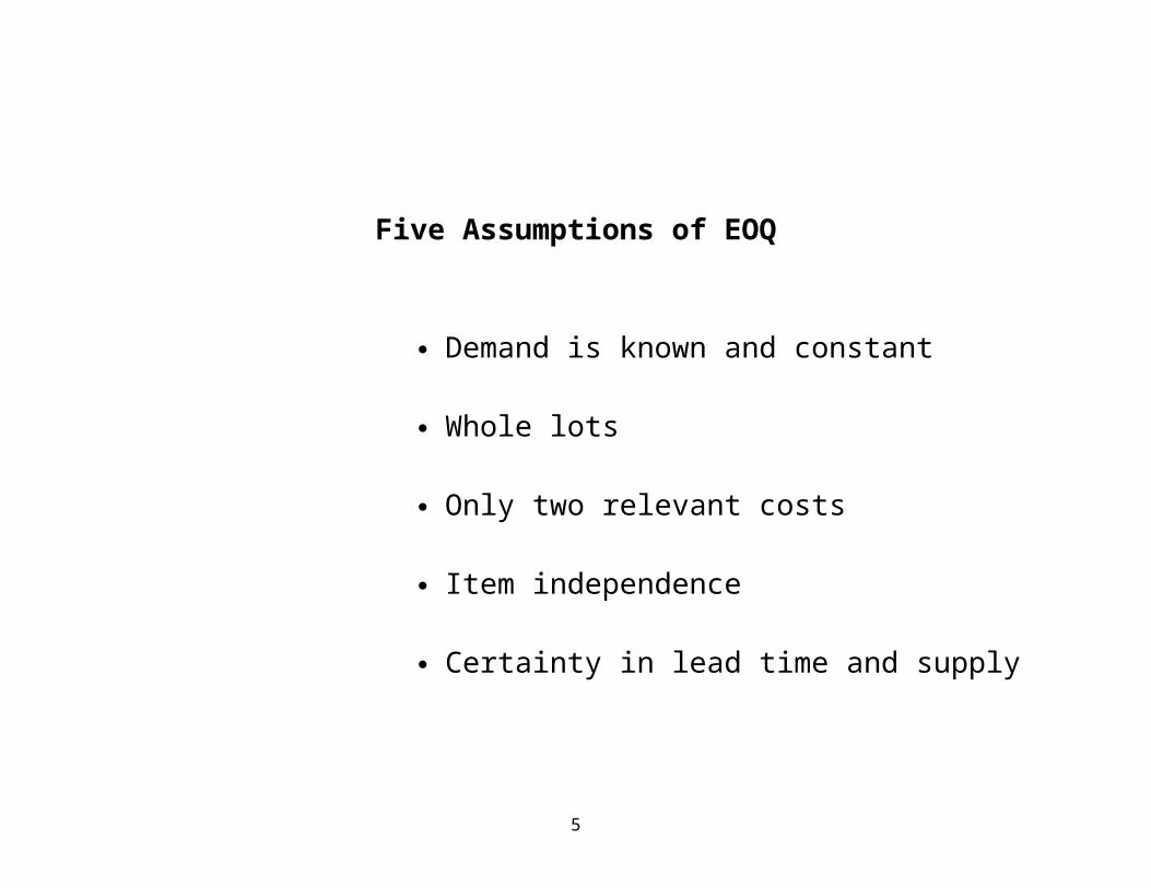
Five Assumptions of EOQ
Demand is known and constant
Whole lots
Only two relevant costs
Item independence
Certainty in lead time and supply
5

Total Annual Relevant Cost
a. Annual holding cost
Annual holding cost =
b. Annual ordering cost
Annual ordering cost =
c. Total annual relevant cost:
Derivation of Economic Order Quantity (EOQ) and Time Between Orders (TBO)
6

Total annual relevant cost: C =
Take the first derivative of cost with respect to quality:
Setting and solving for Q:
Time between orders:
7
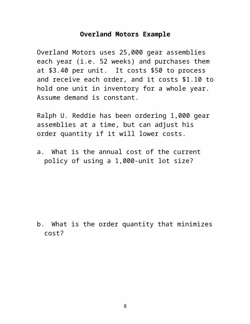
Overland Motors Example
Overland Motors uses 25,000 gear assemblies each year (i.e. 52 weeks) and purchases them at $3.40 per unit. It costs $50 to process and receive each order, and it costs $1.10 to hold one unit in inventory for a whole year. Assume demand is constant.
Ralph U. Reddie has been ordering 1,000 gear assemblies at a time, but can adjust his order quantity if it will lower costs.
a. What is the annual cost of the current policy of using a 1,000-unit lot size?
b. What is the order quantity that minimizes cost?
c. What is the time between orders for the quantity in part b?
d. If the lead time is two weeks, what is the reorder point, R?
8

Economic Production Quantity
1. Maximum Cycle Inventory
2. Total cost = Annual holding cost + Annual ordering or setup cost
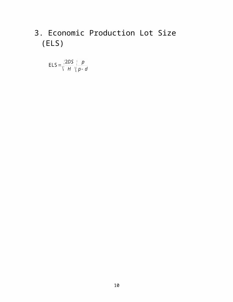
3. Economic Production Lot Size (ELS)
9
Economic Production Quantity Example
A domestic automobile manufacturer schedules 12 two-person teams to assemble 4.6 liter DOHC V-8 engines per work day. Each team can assemble five engines per day. The automobile final assembly line creates an annual demand for the DOHC engine at 10,080 units per year. The engine and automobile assembly plants operate six days per week, 48 weeks per year. The engine assembly line also produces SOHC V-8 engines. The cost to switch the production line from one type of engine to the other is $100,000. It costs $2,000 to store one DOHC V-8 for one year.
a. What is the economic lot size?
b. How long is the production run?
c. What is the average quantity in inventory?
d. What are the total annual relevant costs?
10

Quantity Discounts
In the case of quantity discounts (price incentives to purchase large quantities), the price, P, is relevant to the calculation of total annual cost (since the price is no longer fixed).
Total cost = Annual holding cost + Annual ordering cost + Annual cost of materials
11

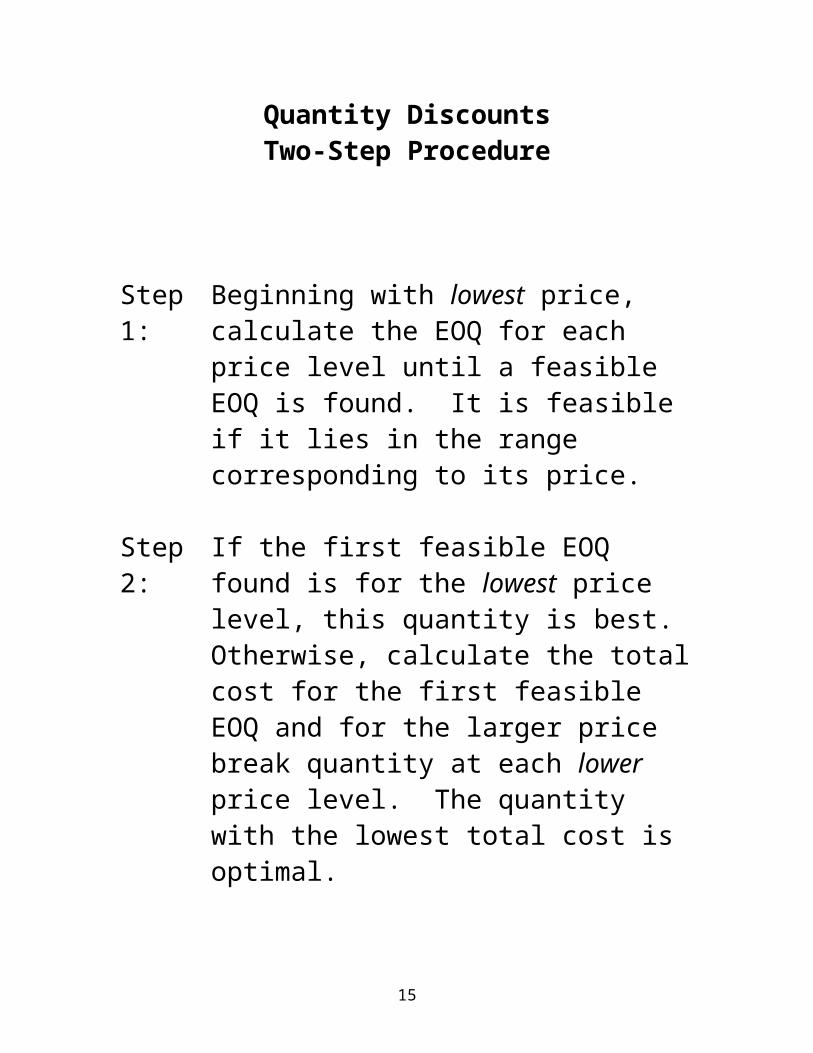
Quantity DiscountsTwo-Step Procedure
Step 1: Beginning with lowest price, calculate the EOQ for each price level until a feasible EOQ is found. It is feasible if it lies in the range corresponding to its price.
Step 2: If the first feasible EOQ found is for the lowest price level, this quantity is best. Otherwise, calculate the total cost for the first feasible EOQ and for the larger price break quantity at each lower price level. The quantity with the lowest total cost is optimal.
12

Quantity Discounts Example
Order Quantity Price Per Unit0-99 $50
100 or more $45
If the ordering cost is $16 per order, annual holding cost is 20 percent of the per unit purchase price, and annual demand is 1,800 items, what is the best order quantity?
Step 1. =
=
Step 2. =
=
13
Reorder Point (Q System)
A continuous review (Q) system tracks the remaining inventory of an item each time a withdrawal is made, to determine if it is time to reorder.
Decision rule: Whenever a withdrawal brings the inventory down to the reorder point (R), place an order for Q (fixed) units.
14
Reorder Point
Demand pattern Lead time for ordering
ROP
Known and constant
None ROP = 0
Known and constant
Known and constant ROP =
Variable, normally distributed, known
Known and constant ROP =
Variable, normally distributed, known
Known and constant ROP =
Known and constant
Variable, normally distributed, known
ROP =
Uncertain, discrete probability distribution
unknown Determine ROP for a given service level based on the cumulative probabilities of demand during lead time.
15

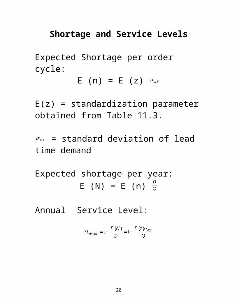
Shortage and Service Levels
Expected Shortage per order cycle: E (n) = E (z)
E(z) = standardization parameter obtained from Table 11.3.
= standard deviation of lead time demand
Expected shortage per year: E (N) = E (n)
Annual Service Level:
16

Q System Example
You are reviewing the company’s current inventory policies for its continuous review system (Q system), and began by checking out the current policies for a sample of items. The characteristics of one item are:
Average demand = 10 units/wk (assume 52 weeks per year) Ordering and setup cost (S) = $45/order Holding cost (H) = $12/unit/year Average lead time (L) = 3 weeks Standard deviation of demand during lead time = 17 units Service-level = 70%
a) What is the EOQ for this item?
b) What is the desired safety stock?
c) What is the desired reorder point R?
d) What is the decision rule for replenishing inventory?
e) What is the expected shortage per year?
If instead of the above situation, suppose the lead time is known and constant at 3 weeks and the standard deviation of demand during lead time is unknown. However, we do know the standard deviation of weekly demand to be 8 units. How do your answers change?
17

Cycle-Service Level with Discrete Distribution
Set R so that the probabilities of demand at or below its level total the desired cycle-service level.
To find safety stock, subtract expected demand during lead time from R.
Application:
The demand during lead time distribution is shown below, along with possible R values and their corresponding cycle-service levels.
DemandLevel Probability R
Cycle-ServiceLevel (%)
0 0.30 050 0.20 50
100 0.20 100150 0.15 150200 0.10 200250 0.05 250
a. What reorder point R would result in a 95% cycle-service level?
b. How much safety stock is provided with this policy?
18

19
Single Period (Newsvendor) Model
Used to handle ordering of perishables and items that have a limited useful life.
shortage costs = unrealized profit per unitexcess costs = the unit cost less the salvage value
1. Calculate the shortage and excess costs:
2. Calculate the service level (SL), which is the probability that demand will not exceed the stocking level:
SL =
3. Determine the optimal stocking level, , using the service level and demand distribution information.
= Mean demand + zSL*demand
20

Example of the Newsvendor Model
The concession manager for the college football stadium must decide how many hot dogs to order for the next game. Each hot dog is sold for $2.25 and makes a profit of $0.75. Hot dogs left over after the game are sold to the student cafeteria for $0.50 each. Based on previous games, the demand is normally distributed with an average of 2000 hot dogs sold per game and a standard deviation of 400. Find the optimal stocking level for hot dogs.
21
Top Related