


Languages
Pages
Legal


Inventory Behavior and the Cost Channel of Monetary Transmission
Gewei Wang∗
September 2011
Abstract
We extend a dynamic New Keynesian model by introducing inventories and convex
adjustment costs to study the cost channel of monetary transmission. We focus on
three empirical observations following a monetary policy shock: (1) swift changes of the
interest rate; (2) slow adjustment of output and inventories; and (3) slow adjustment of
aggregate price. In a model without adjustment costs, the cost channel implies that a
decline in interest rates should reduce firms’ financing costs and motivate them to build
up inventories. Therefore, in order to bring the model’s inventory predictions in line
with the data, we need to assume high costs in capacity adjustment. As a result, the cost
channel leads to a surge in the marginal cost. Calibrating the benchmark model with
the cost channel and adjustment frictions, we find that the resulting impact of monetary
policy on macroeconomic variables is strong in the short run and nonpersistent over the
cycle. We show that two sources of real rigidity help to reconcile high adjustment costs
and price stickiness. These two sources of real rigidity are both relevant to adjustment
frictions. One arises from firms’ motives for dynamic cost smoothing. The other is
related to endogenous marginal cost and strategic complementarity.
JEL classifications: E31 F12
Keywords: Adjustment costs, inventories, monetary shocks, the cost channel
∗Department of Economics, University of California, Berkeley (email: [email protected]). I am greateful toProfessor Yuriy Gorodnichenko, Professor Pierre-Olivier Gourinchas, Professor Maurice Obstfeld, Professor DavidRomer, and all the participants in the Graduate Student Mini Symposium for helpful comments and advice.

1 Introduction
The demand-side transmission mechanism has been explored extensively to identify whether shocks
in monetary policy exert real effects on the economy. Alternatively, some researchers proposed that
the cost-side, or supply-side, channel may be also important1.
The cost channel is analyzed by most of the general equilibrium models2 with the assumption
of intra-period financing: firms must borrow to finance the payments of working capital before they
receive revenues from sales. When, for example, an expansionary shock of monetary policy occurs,
the nominal interest rate declines and financing costs become lower. As a result, the marginal
cost tends to be countercyclical or acyclical. If markups are also countercyclical due to moderate
nominal rigidity, the models imply sluggish price adjustment and large real effects of monetary
policy shocks.
This paper seeks to rethink the cost channel by considering the role of interest rates in the
decision of inventory stocks3. Inventory behavior has implications for monetary transmission by its
very nature. In a theoretical economy where the market clears for each firm’s product, output always
equals demand, so it is difficult to identify whether a change in output is driven by a mechanism
from the demand side or from the supply side. In contrast, inventory investment represents the
difference between sales and output. Investigating inventories thus helps to disentangle these two
transmission channels. In fact, empirical evidence shows that the ratio of inventory to sales is
countercyclical and inventory investment is acyclical the short run, but the cost channel implies
that lower costs should lead to a much higher level of inventory holdings. The inconsistency suggests
that either the cost channel may not be effective or there are strong frictions on the supply side.
We present a New Keynesian model with inventory holdings and adjustment costs to shed light
on the point. We find that high adjustment costs reconcile two empirical observations: swift changes
of financing costs and sluggish adjustment in production and inventories. Inventories can be viewed
as the working capital held and financed for a long period4. In a dynamic model, a decline in the
interest rate raises a firm’s valuation of future production costs and current costs become relatively
low. Therefore, whether for short-term or for long-term financing, interest rate changes have same
effects on production costs and the use of working capital. For example, a decline in the interest rate
due to a monetary expansion should motivate firms to build up inventories. Short-run adjustment
costs thus must be high to reconcile our model with the cyclical behavior of inventories. Otherwise,
if current adjustment costs are low, cost smoothing suggests that future adjustment costs must be
even lower, which cannot be justified in the model with an expansionary shock.
1See Barth and Ramey (2001) for evidence and more references.2For example, see Christiano et al. (2005).3There are mainly two measures of working capital: gross working capital, which is equal to the value of inventories
plus trade receivables; and net working capital, which nets out trade payables.4The turnover period of inventories(the average time a good is held in inventory) used by NIPA is 4 months.
1

We find that the effect of the traditional cost channel on the marginal cost depends on the level
of adjustment costs. The marginal cost is not necessarily high in the presence of high adjustment
costs. It also depends on how strong a firm’s incentive is to adjust output. In a model without
adjustment costs, a decline in interest rates lowers the marginal cost, so the cost channel plays
a cost-restraining role. In a model with adjustment costs, the larger decreases in interest rates,
the larger marginal cost is. Instead, if we shut down the financing cost channel in a model with
adjustment costs, the movement of marginal cost is much less excessive. Our calibration shows that
the responses of macroeconomic variables are less persistent in the benchmark model compared to
the model where inventory holdings are not affected directly by the cost channel of interest rates.
We focus on two sources of real rigidity resulting from adjustment costs. High marginal cost in
the short run pose a challenge to explaining the empirical observation of inflation inertia. However,
the real rigidity discussed in this paper does help to reconcile high adjustment costs with price
stickiness. We find that a transitory rise of marginal cost does not lead to aggressive changes in
price.
We find a new source of real rigidity in the model from the behavior of dynamic cost smoothing.
To our knowledge, this source of real rigidity has not been documented before. In order to reduce
the adjustment costs incurred in the future, firms choose to smooth the process of expanding
production. They start to produce more in order to be prepared to produce more in the future.
For this reason, firms do not have strong incentive to raise price. The nature of adjustment costs
leads to sluggish movement of output, which means that the marginal cost is persistent. In a
model without inventories, we find that this source of real rigidity contributes to both inertia
and persistence of price adjustment. In the inventory model, however, the cyclical behavior of
inventories requires high contemporary costs, so cost smoothing does not play a role in raising real
rigidity. Therefore, if the traditional cost channel through interest rates is not as effective as the
model indicates, adjustment frictions should exert persistent effects on output and inflation through
a new cost channel.
We find that the other real rigidity arising from firm-specific convex adjustment costs plays
an important role in the model. In a Calvo world with pricing frictions, the firms that do not
adjust price in response to rising demand produce less than their expected sales and cut down
inventories. The firms that reoptimize and raise price, meanwhile, curtail sales and build up
inventories. Therefore, the firms with high marginal cost stick to their prices and the firms with
relatively low marginal cost adjust price. This selection effect magnifies countercyclical markups for
aggregate price. The model uses large curvatures of adjustment costs and large price elasticities of
product demand to show how endogenous marginal cost is an important source of large real rigidity.
We show in our calibration that the conflict between high adjustment costs and price stickiness
can be remedied significantly by this source of real rigidity. We solve the model analytically by
linearizing the system of non-linear equations. Because of adjustment frictions and idiosyncratic
2

shocks, different firms have different states. In our model, the optimal behavior of firms depends
on four individual state variables: labor input, the beginning-of-period inventory stock, the end-of-
period inventory stock, and output price. Although the equation system becomes complicated with
more individual state variables, it can be solved by an extension of the undetermined coefficients
method. The approximation procedure clarifies those intuitions, especially the one behind pricing
behavior.
Our model features a motive of stockout avoidance to justify inventory holdings on steady state,
but the main force that determines inventory holdings is through cost smoothing. The reason is
that the depreciation rate of inventories is rather small in calibration and the benefit of stockout
avoidance only accounts for a small part in determining inventory holdings. Our results are robust
to the parameterization because due to a shock of demand boom the motive of stockout avoidance
becomes also stronger, albeit not associated with the traditional cost channel.
The paper is organized as follows. Section 2 summarizes related literature. Section 3 reports
basic findings of inventory behavior conditional on a monetary policy shock. Section 4 discusses
the relationship between adjustment costs and pricing behavior by presenting a baseline model
that introduces convex adjustment costs of labor input to an otherwise standard New Keynesian
model. Section 5 develops the baseline model by adding to the model inventory holdings. Section
6 describes calibrated results and compares them with other models. This section also discusses
some results of robustness checks and possible extensions. Section 7 concludes.
2 Related literature
This paper is related to a large body of literature that studies the behavior of price rigidity, inven-
tories5, and costs over the business cycle. Our starting point is the observation of sluggish output
adjustment in the short run from recent evidence of VARs and identified monetary shocks. This can
be seen as indirect evidence of countercyclical inventory movement because inventory investment
accounts for the difference between sales and output. Standard recursive vector autoregressions
(VARs) indicate that real GDP, hours worked, and investment barely move in the first quarter in
response to a monetary policy shock, but sales and consumption do (for example, see figure 3 in
Christiano, Trabandt, and Walentin, 2010). The output adjustment estimated with an identified
shock is even more sluggish. Figure 2 in Romer and Romer (2004) shows that industrial pro-
duction has not started to fall until six months after a monetary contractionary. Direct evidence
by including inventory explicitly in the VAR also supports this result. Figure 2 in Bernanke and
Gertler (1995) shows that inventories appear to build up for 8 months before beginning to decrease
5Inventory movements play a major role in business cycle fluctuations although the level of inventory investmentis less than 0.5% of GDP in developed countries. For example, Ramey and West (1999) document that, for quarterlyUS data, the decline of inventory investment accounts for 49 percent of the fall in GDP for the 1990-1991 recessionand on average 69 percent of the fall in GDP for the postwar recessions during the period from 1948 to 1991.
3

following an unanticipated tightening of monetary policy. Gertler and Gilchrist (1994), Jung and
Yun (2005) and many others have all confirmed countercyclical or acyclical movement of inventory
holdings over the business cycle. Bils and Kahn (2000) emphasize countercyclical inventory-to-sales
ratios. They find in the long run inventories do track sales one for one, but the ratio of inventory
to sales is highly persistent and countercyclical, which implies output does not keep pace with sales
in the short run6.
For the traditional cost channel, previous literature mainly studies the effect of intra-period
financing, so the change of interest rates directly affects marginal cost. Christiano et al. (2005)
argue that the cost decline from intra-period borrowing of payroll helps to explain the odd behavior
of inflation after a monetary policy shock7. The credit channel of financial accelerator proposed
by Bernanke and Gertler (1989) has been tested extensively using the evidence from inventory
behavior over the business cycle. Gertler and Gilchrist (1994) find that financial factors play a
prominent role in the slowdown of inventory demand as monetary policy tightens. They compare
inventory behavior across size classes and confirm that small firms exhibit a greater propensity to
shed inventories as sales drop. This suggests that financial costs are at work through the effect of net
worth when firms make decisions on their inventory holdings. Kashyap, Stein, and Wilcox (1993)
and Kashyap, Lamont, and Stein (1994) provide time-series and cross-sectional empirical evidence
that a significant number of firms are bank-dependent and therefore have inventory behavior that
is sensitive to bank lending conditions.
The literature that studies the incentives to hold inventories has evolved substantially since the
1980s. In general, the incentives in most models are cost reduction, sales benefit, or both. After
noticing the empirical inconsistency of the production smoothing theory, one strand of inventory
research is to add to the model a targeted inventory level or inventory-to-sales ratio; for example, the
target can be determined by the motive of stockout avoidance (Kahn, 1987), direct sales promotion
(Bils and Kahn, 2000), or cost uncertainty (Wang and Wen, 2009). The alternative explanation is
the (S, s) theory first brought into the macroeconomic scope by Caplin (1985)8. Khan and Thomas
(2007) develop an equilibrium business cycle model driven by technology shocks where nonconvex
delivery costs lead firms to follow (S, s) inventory policies. In such a real model, markups are
constant. As Kryvtsov and Midrigan (2010b) argue, if markups are constant, monetary shocks can
6The main difference between VAR results and that of Bils and Kahn is that they use a partial equilibrium modelof inventories to reveal the cyclicality of real marginal cost over the business cycle, not specific to a monetary shock.
7A dip during the first several quarters.8The (S, s) theory considers adjustment behavior in the presence of non-convex costs. If adjustment costs is
simply fixed costs incurred at any time a firm wishes to adjust its inventories, Scarf (1960) shows that the firm’soptimal decision rule takes a one-sided (S, s) form. On the one hand, (S, s) policy has different implication frominventory targeting in that high or low inventory levels do not pertain to the marginal cost of inventory. On theother hand, inventory targeting with convex adjustment costs indicates that if inventory cannot keep pace with sales,the marginal cost of replenishing inventories must increase. Although the (S, s) model has also received considerableattention, due to the cumbersome heterogeneity across firms, it was not until Khan and Thomas (2007) and Kryvtsovand Midrigan (2009) that (S, s) inventory policy is incorporated into a general equilibrium model to analyze businesscycles. However, the models must be solved using numerical methods.
4

only generate real effects only if nominal costs are sticky, which gives rise to strong variability in
inventories due to intertemporal substitution in production; this result, however, is at odds with
the data.
Sluggish output adjustment implies the existence of adjustment frictions. Most macroeconomic
research, until recently, has used convex cost functions to slow down changes with rising marginal
cost9. Although some microeconomic studies argue that firm-level lumpy adjustment of capital and
inventory stocks may favor the explanation of non-convex costs, or in a narrower sense, fixed costs,
the results in Kryvtsov and Midrigan (2009, 2010a) seem to suggest this choice of cost functions
does not affect price stickiness significantly10. After all, it is hard to think that adjustment frictions
are irrelevant to a firm’s marginal cost. Our New Keynesian model assumes a convex cost function
to represent the source of all frictions in production adjustment.
Recent attempts to include inventory in a standard New Keynesian model focus on the nomi-
nal and real rigidity required to achieve observed inflation inertia. Jung and Yun (2005) develops
a general equilibrium model that follows Bils and Kahn (2000), in which the motive of holding
inventories is to promote sales. Their model also includes a sector which does not use invento-
ries. They find that very high nominal rigidity is required to accommodate both countercyclical
inventory-to-sales ratios and price rigidity in the model.
Our inventory model is based on Kryvtsov and Midrigan (2009, 2010a,b), which provide a thor-
ough study of inventory behavior and real rigidity. They construct a model of stockout avoidance
to rationalize inventory holdings, together with Calvo pricing, or menu cost. They conclude that
the interest rate change in response a monetary policy shock invokes a strong motive of intertempo-
ral substitution and that standard parameterization cannot reconcile inventory behavior and price
rigidity. Kryvtsov and Midrigan (2010b) introduce firm-level decreasing returns to generate suffi-
cient real rigidity and focus on the measure of how much nominal cost rigidity and countercyclical
markups account for the bulk of the real effects of monetary policy shocks. We place emphasis
on the implication for the traditional cost channel of monetary transmission. Inventory behavior
suggests that the cost channel may not be effective or there are frictions on the supply side. Our
model focuses on heterogeneous adjustment costs among firms. We show that in a Calvo world
with pricing frictions, the firms that do not adjust price in response to rising demand produce less
than their expected sales and cut down inventories. The firms that reoptimize and raise price,
meanwhile, curtail sales and build up inventories. Therefore, the firms with high marginal cost
stick to their prices and the firms with relatively low marginal cost adjust price. This selection
effect implies that a large nominal rigidity may not be required to reconcile real rigidity.
In stockout avoidance models, holding more inventories increases expected sales. Ex post stock-
out happens for only a few firms and inventory stocks are exhausted only for these firms. However,
9For a survey for theoretical applications and empirical performance of convex costs, see Khan and Thomas (2008).10See Kryvtsov and Midrigan (2009, 2010a) for detailed discussion.
5

the ex ante benefit of inventory for sales is the same for all firms. In this sense, inventory behav-
ior in the models of sales promotion and stockout avoidance does not make much difference. In
this paper, it turns out that, after an expansionary monetary policy shock, the shadow value of
inventory stock is primarily determined by the motive of inter-temporal substitution, not by any
additional form of benefit.
Recent work of New Keynesian models introduces real rigidity in two ways. The first is internal
real rigidity characterized by a price increase associated with a decline in marginal cost at the
firm level. Several examples include countercyclical price elasticity (Kimball, 1995; Eichenbaum
and Fisher, 2007), diminishing returns to scale (Gali, 2008; Kryvtsov and Midrigan, 2010b), firm-
specific capital (Altig et al., 2011), and firm-specific labor (Woodford, 2003). The second approach
is external real rigidity that reduces the responsiveness of real marginal cost at the aggregate level.
One widely used approach is sticky wages (Erceg et al., 2000; Christiano et al., 2005; Smets and
Wouters, 2007). As a matter of fact, medium-sized dynamic stochastic general equilibrium (DSGE)
models usually include both sources of real rigidity. Two sources of real rigidity in our model fall
into the first category. The first is firm-specific convex costs, which exerts a effect similar to firm-
specific factors. The second is dynamic adjustment friction that is distinct from all other real
rigidity.
3 Evidence from identified monetary policy shocks
Since the focus of this paper is on the real effect of monetary policy shocks, we document the
behavior of inventory and sales in the wake of monetary expansions and contractions. A necessary
step here is to identify these monetary disturbances. We use the monthly NIPA data which contain
high-frequency observations. Output is computed as the sum of real sales and inventory investment
for the manufacturing and sales industry. The price level is measured using implicit price deflators
for sales. Our measure of monetary shocks represents innovations to the intended fed funds rate
due to Romer and Romer (2004) (R&R), which is based on narrative records of FOMC meetings
and Federal Reserve’s internal forecasts.
Responses of output, price levels, inventory investment and inventory-sales ratios are obtained
by estimating the following OLS regression:
∆yt = a0 +
11∑k=1
akDkt +
24∑i=1
bi∆yt−i +
36∑j=1
cjSt−j + et,
where yt is the dependent variable, Dk’s are a full set of monthly dummies, S is the measure of
Romer-Romer shocks, and et is the zero-mean normally distributed error term, which is assumed
to be serially uncorrelated. This specification is used by R&R and implies policy shocks have no
contemporary effect on macroeconomic variables. To be consistent with this assumption, the same
6

timing restriction will be applied in our model. Our analysis for robustness check in section 5 shows
that this assumption is essentially innocuous for the responses of most variables.
Figure 1 reports impulse responses to R&R shocks. The solid lines in the figure denote point
estimates of the different response functions, and the dashed lines report respective 95% confidence
intervals computed by bootstrapping. Output responses are negative between 4 and 36 months,
with the trough at around 24 months after the shock. The response of inventory investment
is countercyclical for about one year after the shock, reflecting the fact that inventory stocks are
adjusted with a lag. We corroborating the result of countercyclical inventory-sales ratios conditional
on a monetary policy shock: after a contractionary monetary shock, the ratio rises until one and a
half year later.
Figure 2 and Figure 3 show the responses for the manufacturing industry and the trade industry
separately. Inventory investment is countercyclical for the manufacturing industry during the first
18 months, but only acyclical for the trade industry during the first year after the shock. Figure
4 breaks down inventories according to three processing stages. Basically, the patterns are similar
across different stages.
[Figure 1, 2 ,3, and 4 here]
[Figure 5 here]
4 Adjustment costs and pricing in a baseline model
4.1 A simple example
This section illustrates the relationship between adjustment costs and pricing behavior. We start
with a stylized example showing how heterogeneous adjustment costs across firms contributes higher
real rigidity at the aggregate level. Consider an economy with a continuum of firms, whose optimal
pricing decisions are characterized by the following log-linearized best-response:
pi − p = mci
where pi denotes firm i’s optimal price, p =∫pidi denotes the average price of all firms, and mci
denotes firm i’s marginal cost. This equation can be derived from a static pricing strategy with a
constant markup. When individual marginal cost is determined only by aggregate output y, that
is, mci = ξy, the equation can be rewritten as
pi = ξ(p+ y) + (1− ξ) p, ξ > 0
Given a certain level of nominal rigidity, after a shock of nominal spendings, the closer ξ is to zero,
the more sluggish price adjustment is. When individual marginal cost is a decreasing function of
7

relative product price: mci = ξy − η (pi − p), η > 0, we have
pi =ξ
1 + η(p+ y) +
1 + η − ξ1 + η
p, ξ > 0 and η > 0
which implies that if a firm’s marginal cost is sensitive to its relative product price, large real
rigidity is possible. In our model to be formulated below, this measure η essentially depends on the
price elasticity of demand and the curvature of cost functions. Because aggregate marginal cost
mc ≡∫mcidi, defined here as the average of individual marginal cost, still equals ξy, we call ξ a
measure of external real rigidity and η a measure of internal real rigidity.
Consider adjustment costs in the model. If individual adjustment costs are completely de-
termined at the industry level when mci does not depend on pi, price stickiness requires that
aggregate adjustment costs must be low (small ξ). However, if adjustment costs are heterogeneous
across firms, they decrease with relative price (η > 0). Each reoptimizing firm sets price based on
individual marginal cost, which will be unambiguously lower than aggregate marginal cost if price
is lifted up.
We continue to explain this selection effect in this section by presenting a general equilibrium
model. All elements in the model follow medium-sized New Keynesian models such as in Christiano
et al. (2005), except for convex adjustment costs of labor inputs to shed light on our intuition.
4.2 A New Keynesian model with labor adjustment costs
In the baseline model with two factors in production, differentiated goods are produced by a
continuum of monopolistically competitive firms, indexed by i ∈ [0, 1], using a Cobb-Douglas
production function:
Yt (i) = Kαt (i)Lt (i)1−α
where Yt (i) denotes individual output of firm i at period t, Lt (i) denotes labor input in production,
and Kt (i) denotes the input of capital service. A firm needs to hire Υ(
Lt(i)Lt−1(i)
)Lt (i) units of labor
to adjust employment in production. Υ (·) is a convex cost function of labor adjustment such that
Υ (1) = Υ′ (1) = 0 and Υ′′ (1) > 0. The real cost function therefore includes a component of labor
adjustment costs:WtPtLt (i) + Wt
PtΥ(
Lt(i)Lt−1(i)
)Lt (i) +RK,tKt (i)
where Pt is the price index, Wt is nominal wage, and RK,t is the rental rate of capital service. The
demand curve for one firm is given by
Yt (i) =
(Pt (i)
Pt
)−θCt
where Ct denotes aggregate consumption.
8
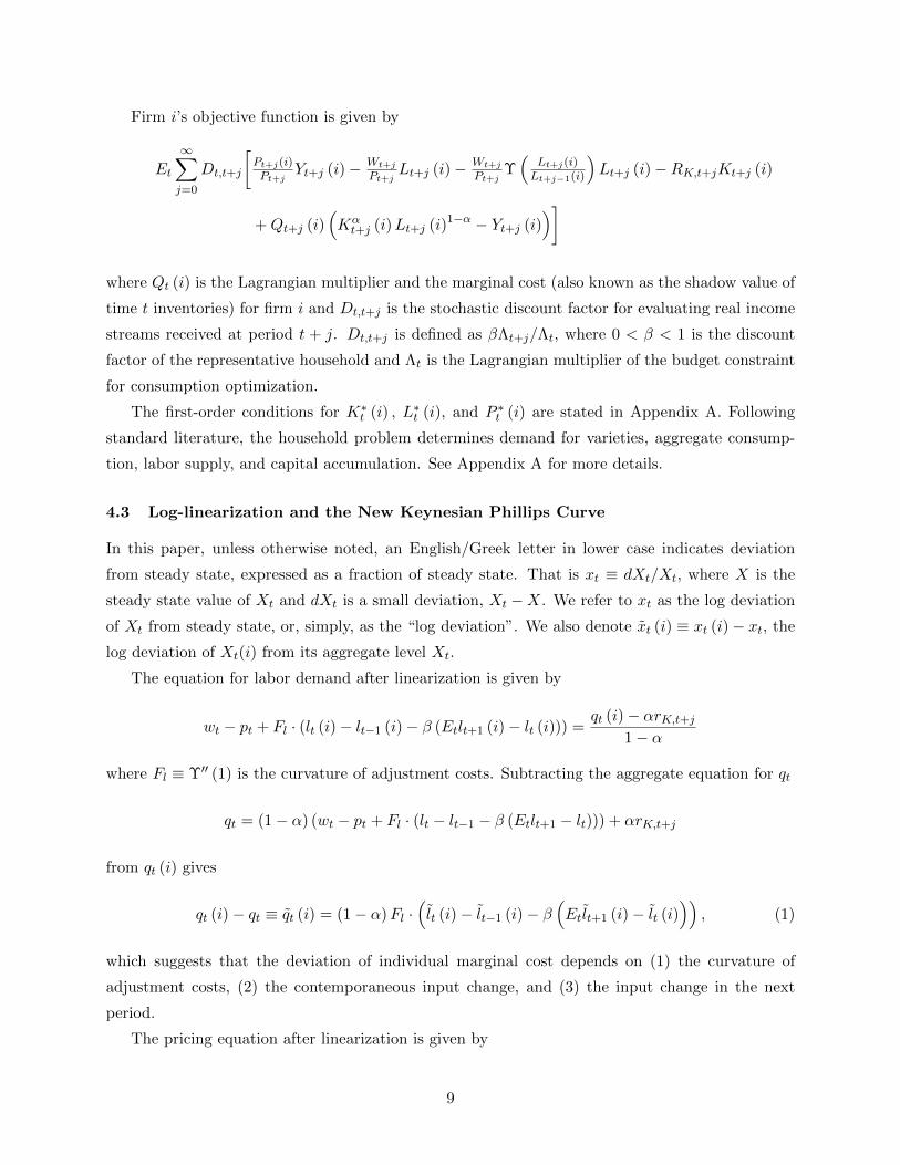
Firm i’s objective function is given by
Et
∞∑j=0
Dt,t+j
[Pt+j(i)Pt+j
Yt+j (i)− Wt+j
Pt+jLt+j (i)− Wt+j
Pt+jΥ(
Lt+j(i)Lt+j−1(i)
)Lt+j (i)−RK,t+jKt+j (i)
+Qt+j (i)(Kαt+j (i)Lt+j (i)1−α − Yt+j (i)
)]
where Qt (i) is the Lagrangian multiplier and the marginal cost (also known as the shadow value of
time t inventories) for firm i and Dt,t+j is the stochastic discount factor for evaluating real income
streams received at period t + j. Dt,t+j is defined as βΛt+j/Λt, where 0 < β < 1 is the discount
factor of the representative household and Λt is the Lagrangian multiplier of the budget constraint
for consumption optimization.
The first-order conditions for K∗t (i) , L∗t (i), and P ∗t (i) are stated in Appendix A. Following
standard literature, the household problem determines demand for varieties, aggregate consump-
tion, labor supply, and capital accumulation. See Appendix A for more details.
4.3 Log-linearization and the New Keynesian Phillips Curve
In this paper, unless otherwise noted, an English/Greek letter in lower case indicates deviation
from steady state, expressed as a fraction of steady state. That is xt ≡ dXt/Xt, where X is the
steady state value of Xt and dXt is a small deviation, Xt −X. We refer to xt as the log deviation
of Xt from steady state, or, simply, as the “log deviation”. We also denote x̃t (i) ≡ xt (i)− xt, the
log deviation of Xt(i) from its aggregate level Xt.
The equation for labor demand after linearization is given by
wt − pt + Fl · (lt (i)− lt−1 (i)− β (Etlt+1 (i)− lt (i))) =qt (i)− αrK,t+j
1− α
where Fl ≡ Υ′′ (1) is the curvature of adjustment costs. Subtracting the aggregate equation for qt
qt = (1− α) (wt − pt + Fl · (lt − lt−1 − β (Etlt+1 − lt))) + αrK,t+j
from qt (i) gives
qt (i)− qt ≡ q̃t (i) = (1− α)Fl ·(l̃t (i)− l̃t−1 (i)− β
(Et l̃t+1 (i)− l̃t (i)
)), (1)
which suggests that the deviation of individual marginal cost depends on (1) the curvature of
adjustment costs, (2) the contemporaneous input change, and (3) the input change in the next
period.
The pricing equation after linearization is given by
9

pt (i)− pt ≡ p̃t (i) = (1− αpβ)Ep̄t
∞∑j=0
(αpβ)j qt+j (i) + Ep̄t
∞∑j=1
(αpβ)j ∆%πt+j . (2)
The inflation rate is denoted by πt ≡ logPt − logPt−1. If a firm does not change price during the
period from t to t+ j, since qt+j (i) is determined by lt+j (i), and then pt−1 (i), pt (i) is a function
of pt−1 (i). We posit that
p̃t (i) = ψp̃t−1 (i) + p∗t
Intuitively, ψ is larger than zero because if input is low in last period, to avoid high adjustment
costs, input today still stays low; ψ should also be less than one because of the requirement of
system stationarity. It follows that individual marginal cost is determined by
q̃t (i) = (1− α)Flε (p̃t−1 (i)− φp̃t (i))
where
φ ≡ 1 + β (1− αp − (1− αp)ψ)
We find that the function of individual marginal cost is decreasing with individual product price
as φ > 0, which is consistent with our stylized example. Therefore, aggregating the re-optimized
prices gives
p∗t = Ep̄t
∞∑j=1
(αpβ)j ∆%πt+j
+ (1− αpβ)Ep̄t
∞∑j=0
(αpβ)j qt
new { −ε (1− α)Fl (φ− αpβ)
p∗t − Ep̄t ∞∑j=1
(αpβ)j ∆%πt+j
(3)
where the third line is new due to the introduction of adjustment costs. After simplification, the
New Keynesian Phillips Curve is given by
∆%πt =(1− αpβ) (1− αp)
αp
1
1 + κqt + βEt∆%πt+1,
where
κ ≡ ε (1− α)Fl · (φ− αpβ)
Here κ is a measure of real rigidity resulted from adjustment costs. κ has a lower bound of zero
when there are no adjustment costs. It depends basically on the value of ε and Fl since φ − αpβis close to 1 in our calibration. Because Fl < 5 is fairly reasonable, κ can be considerably large.
10
Figure 6 shows the relationship between κ and Fl. When Fl is above 1, κ is approximately more
than 4.
[Figure 6 here]
The intuition of the selection effect can be seen in equation (3). A firm’s price is based on its
own marginal cost. As individual marginal cost is endogenous, it increases with output, thereby
decreases with relative price. When output is elastic with price and adjustment friction is high,
individual marginal cost is responsive to product price, which thereby responds less to aggregate
marginal cost.
The effect of large firm-specific adjustment costs on the inflation response is through two chan-
nels. The first is through higher κ, which increases strategic complementarity in pricing and
therefore inflation responds less to a change of aggregate marginal cost. The second is through qt:
the higher individual adjustment costs, the higher aggregate marginal cost is. Figure 8 shows the
impulse responses after an expansionary monetary policy shock11. The inflation response with a
larger cost curvature is even flatter. Because aggregate price is determined by re-optimizing firms,
this means they charge even lower prices when they face higher wage rates and adjustment costs.
The selection effect cannot explain this puzzling behavior. However, we can find clues from the
dynamic structure of adjustment costs. Equation (1) shows firms need to take into consideration
future adjustment costs. When firms are sluggish in adjusting price, they wish to adjust input
quickly in order to reduce expected adjustment costs in the future. In our calibration, the optimal
price is even lower for larger adjustment costs. As a result, the effect of enlarged real rigidity
dominates the effect of rising aggregate marginal cost, and price adjustment is more sluggish.
The source of real rigidity arising from dynamic cost smoothing is a novel idea. In order to
smooth adjustment costs, firms choose to increase input purchase immediately after an expansionary
shock instead of raising price. They start to produce more in order to be prepared to produce more
in the future. This motive for inter-temporal substitution is different from other sources of real
rigidity like strategic complementarity among firms or counter-cyclical markups that works intra-
temporally12.
[Figure 8 here]
5 A model with inventories
We formulate in this section a New Keynesian model with inventories. The motive of stockout
avoidance is introduced to justify positive inventory holdings on steady state. We solve the model
analytically by linearizing the system of non-linear equations. Adjustment frictions imply different
firms have different states. In our model, the optimal behavior of firms depends on four individual
11See Appendix A for the parametrization based on quarterly data12The selection effect is one example of this.
11

state variables: labor input, the beginning-of-period inventory stock, the end-of-period inventory
stock, and output price. Although the equation system becomes complicated with more individual
state variables, it can be solved by an extension of the undetermined coefficients method. The
benefit of this approximation procedure is to clarify intuitions, especially the one behind pricing
behavior.
5.1 Household
We denote vt (i) as a preference shock specific to each good in the CES aggregator. Assume
log (vt) ∼ N(−σ2
v2 , σ
2v
). The preference shocks at each period unfold to all firms after they make
decisions on the quantity of goods supplied to the market. Therefore, in this economy the represen-
tative consumer’s demand will occasionally be satisfied in part by firms with insufficient inventory
available. We let Zt (i) be each firm’s available stock of inventories: the consumer cannot buy more
than Zt (i) units. The consumer’s optimization problem is defined as
max E0
∞∑t=0
βtU (Ct, Nt)
st.
∫ 1
0Pt (i)Ct (i) di+ EtDt,t+1Bt+1 ≤ Bt +WtNt + Πt
where
Ct (i) ≤ Zt (i)
Ct =
(∫ 1
0vt (i)
1θ Ct (i)
θ−1θ di
) θθ−1
Bt+1 denotes a portfolio of nominal state contingent claims in the complete contingent claims
market, Dt,t+1 denotes the stochastic discount factor for computing the nominal value in period t
of one unit of consumption goods in period t+ 1, Wt denotes aggregate nominal wage, Nt denotes
labor supply, and Πt denotes a lump-sum transfer.
The inter-temporal Lagrangian is given by
L = E0
∞∑t=0
βt(U (Ct, Nt) + Λt
(WtNt −
∫ 1
0Pt (i)Ct (i) di
)+
∫ 1
0µt (i) (Zt (i)− Ct (i)) di
)
where Λt is the multiplier on the consumer’s budget constraint and µt (i) are the multipliers on the
constraint Ct (i) ≤ Zt (i) for all i.
12
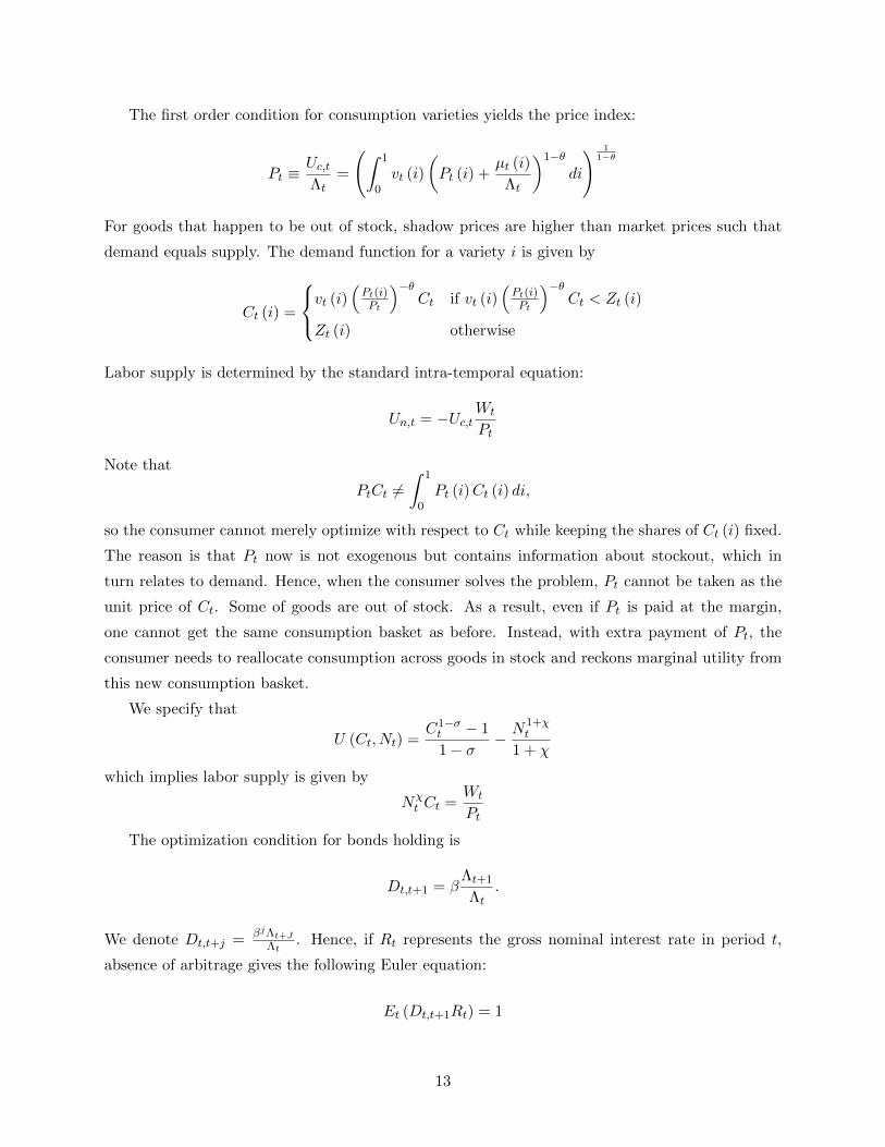
The first order condition for consumption varieties yields the price index:
Pt ≡Uc,tΛt
=
(∫ 1
0vt (i)
(Pt (i) +
µt (i)
Λt
)1−θdi
) 11−θ
For goods that happen to be out of stock, shadow prices are higher than market prices such that
demand equals supply. The demand function for a variety i is given by
Ct (i) =
vt (i)(Pt(i)Pt
)−θCt if vt (i)
(Pt(i)Pt
)−θCt < Zt (i)
Zt (i) otherwise
Labor supply is determined by the standard intra-temporal equation:
Un,t = −Uc,tWt
Pt
Note that
PtCt 6=∫ 1
0Pt (i)Ct (i) di,
so the consumer cannot merely optimize with respect to Ct while keeping the shares of Ct (i) fixed.
The reason is that Pt now is not exogenous but contains information about stockout, which in
turn relates to demand. Hence, when the consumer solves the problem, Pt cannot be taken as the
unit price of Ct. Some of goods are out of stock. As a result, even if Pt is paid at the margin,
one cannot get the same consumption basket as before. Instead, with extra payment of Pt, the
consumer needs to reallocate consumption across goods in stock and reckons marginal utility from
this new consumption basket.
We specify that
U (Ct, Nt) =C1−σt − 1
1− σ− N1+χ
t
1 + χ
which implies labor supply is given by
Nχt Ct =
Wt
Pt
The optimization condition for bonds holding is
Dt,t+1 = βΛt+1
Λt.
We denote Dt,t+j =βjΛt+J
Λt. Hence, if Rt represents the gross nominal interest rate in period t,
absence of arbitrage gives the following Euler equation:
Et (Dt,t+1Rt) = 1
13

5.2 Firms
5.2.1 Production function, inventory, and goods demand
Storable final goods are produced by monopolistically competitive firms using a production function
linear in labor:
Yt (i) = exp(eAt)Lt (i)
where Yt (i) denotes individual output of firm i at period t, Lt (i) denotes labor input, and eAt
represents the technology shock with zero mean. Goods are storable and can be held as finished
goods inventory. A firm needs to hire Υ(
Lt+j(i)Lt+j−1(i)
)Lt (i) units of labor to adjust employment in
production. Υ (·) is a convex cost function of labor adjustment such that Υ (1) = Υ′ (1) = 0 and
Υ′′ (1) > 0. Hence, the cost function of production is given by
C (Yt (i)) = Wt
(Lt (i) + Υ
(Lt(i)Lt−1(i)
)Lt (i)
)Firms cannot observe idiosyncratic demand shocks before production, therefore, inventory can
be used to ensure market clearing. Denote sales by S. It is possible that sales do not equal output
for individual firms and the economy: St (i) 6= Yt (i) and St 6= Yt. The demand function for firm i
is given by
St (Pt (i) , Zt (i)) = min
(vt (i)
(Pt (i)
Pt
)−θCt, Zt (i)
)The beginning-of-period inventory stock of firm i evolves over time according to
Zt (i) = (1− δ) (Zt−1 (i)− St−1 (i)) + Yt (i)− Ξ(
Zt(i)Zt−1(i)
)Zt (i)
where Zt (i) is defined as inventory holdings at the beginning of period t after production, and δ is
the constant marginal cost of inventory stocks measured in the form of iceberg loss. Ξ(
Zt(i)Zt−1(i)
)Zt (i)
is a convex function of inventory adjustment costs such that Ξ (1) = Ξ′ (1) = 0 and Ξ′′ (1) > 0.
Inventory costs can take several forms. Besides natural attrition, storage and maintenance costs
are incurred when a firm stocks and moves inventory. External financing premium is also one main
type of inventory costs if a firm borrows short-term loans to finance inventory holdings.
Consumers cannot resell the goods purchased, thus they do not choose to store goods because
the expected return is negative while we assume the riskfree rate is always positive. In the literature,
there are basically two benefits to induce firms to hold inventories on steady state when firms may
face idiosyncratic shocks but no aggregate shocks: cost reduction and sales promotion. The DSGE
inventory models of cost reduction include idiosyncratic cost uncertainty (Wang and Wen, 2009)
and (S, s) policy for fixed ordering cost (Khan and Thomas, 2007). Sales promotion models can
be specified with the motive of stockout avoidance (Kryvtsov and Midrigan, 2009, 2010a,b) by
14

idiosyncratic demand uncertainty, which our model is based upon. Because the rate of inventory
depreciation cannot be very large, after an expansionary monetary policy shock, the increase of
benefit from sales promotion is relatively small and it turns out that the shadow value of inventory
stock is primarily affected by the decline of interest rates. In this case, the motive of (aggregate)
cost smoothing dominates any other incentives for firms to determine the optimal level of inventory
stocks. As we will see, this cost structure has profound implications on inventory behavior.
5.2.2 Objective function and optimal conditions
Firms set prices according to a variant of the mechanism spelled out by Calvo (1983). In each
period, a firm faces a constant probability, αp, of not being able to re-optimize its nominal price.
L = Et
∞∑j=0
Dt,t+j
[Pt+j (i)St+j (i)−Wt+j (i)Lt+j (i)−Wt+j (i) Υ
(Lt+j(i)Lt+j−1(i)
)Lt+j (i)
+Qt+j (i)(
(1− δ) (Zt+j−1 (i)− St+j−1 (i)) + Lt+j (i)− Zt+j (i)− Ξ(
Zt(i)Zt−1(i)
)Zt (i)
)]
where Qt (i) is the Lagrangian multiplier and the shadow value of time t inventory for firm i.
Here we have two types of convex adjustment costs: Υ (·) for labor input adjustment and Ξ (·) for
inventory stock adjustment. δ denotes the rate of one-period inventory depreciation.
The first-order conditions for Zt (i) , Lt (i), and Pt (i) can be summarized as follows. Firms that
do not re-optimize prices simply follow the indexation rule. Therefore, the optimal condition of
pricing is only applied to those firms that re-optimize.
The first-order condition for inventory holdings Zt (i) is given by
Qt (i)(
1 + Ξ′(
Zt(i)Zt−1(i)
)Zt(i)Zt−1(i) + Ξ
(Zt(i)Zt−1(i)
))− EtDt,t+1Qt+1 (i) Ξ′
(Zt+1(i)Zt(i)
)(Zt+1(i)Zt(i)
)2
= Pt (i) ∂EtSt(i)∂Zt(i)+ Et (1− δ)Dt,t+1Qt+1 (i)
(1− ∂EtSt(i)
∂Zt(i)
)(4)
This equation defines a dynamic equation for inventory holdings. The left hand side is the marginal
cost of accumulating one unit of inventory at period t. The right hand side comes from the benefit
of sales promotion and the discounted marginal cost at period t+ 1. If demand is less than stocks,
inventory leftovers must be restocked. Intertemporal cost smoothing considers the future shadow
value of inventory which reflects the storage role of inventory. The first-order conditions for labor
input Lt (i) is given by
Qt (i) = Wt
(1 + Υ′
(Lt(i)Lt−1(i)
)Lt(i)Lt−1(i) + Υ
(Lt(i)Lt−1(i)
))− EtDt,t+1Wt+1Υ′
(Lt+1(i)Lt(i)
)(Lt+1(i)Lt(i)
)2
which shows that the shadow value of production equals marginal cost. In our model, marginal
15

cost of production also includes adjustment costs of labor input. The first-order conditions for
price-setting Pt (i) is given by
Ep̄t
∞∑j=0
αjpDt,t+jSt+j (i)
Pt+j (i)
[Pt+j (i)− εt+j (i)
εt+j (i)− 1(1− δ)Dt+j,t+j+1Qt+j+1 (i)
]= 0
where εt+j (i) ≡ −Pt+j(i)EtSp̄p,t+j(i)
Rt+j(i). This equation describes a standard pricing equation with Calvo
frictions. The markup becomes time-varying when inventory is considered. In addition, pricing
is based on the discounted marginal cost of the following period in the equation because of cost
smoothing indicated in equation (4).
Note that Et and Ep̄t are different operators because the expectations are conditional on different
events. Ep̄tXt+k (i) denotes the expectation of the random variable Xt+k (i) , condition on date t
information and on the event that firm i optimizes its price in period t, but does not do so in
any period up to and including t + k. For any aggregate state variable Xt+k, Ep̄tXt+k = EtXt+k.
However, the two conditional expectations differ for firm i’s individual variables. This distinction
is emphasized in Woodford (2005).
5.3 Social resource constraint and monetary policy
The aggregate production equation and labor market clearing imply that
Yt +
∫ 1
0Υ(
Yt(i)Yt−1(i)
)Yt (i) di = Nt
Aggregating individual inventory holdings gives us the law of motion for aggregate inventory stock
Zt = (1− δ) (Zt−1 − St−1) + Yt −∫ 1
0Ξ(
Zt(i)Zt−1(i)
)Zt (i) di. (5)
One can see that the aggregate market clearing condition can be written as
Yt = St + IZ,t (6)
where IZ,t ≡ Zt−St− (1− δ) (Zt−1 − St−1)−∫ 1
0 Ξ(
Zt(i)Zt−1(i)
)Zt (i) di denotes inventory investment.
Finally, the monetary policy rule is assumed to follow a variant of Taylor (1993) rule with partial
adjustment of the form
log
(RtR
)= ρr log
(Rt−1
R
)+ (1− ρr)
(ρππt + ρy log
(YtY
))+ ert , (7)
where ρr is the partial adjustment parameter, ρπ measures the responsiveness of the policy interest
rate with respect to inflation rate, ρy measures the responsiveness of the policy interest rate with
16

respect to real output, and ert is an exogenous (possible stochastic) component with zero mean. It
is also assumed that it takes one period for private agents to observe monetary shocks, so ert is not
included in the period t information set of the agents in the model. This ensures that the model
satisfies the restriction used in the empirical analysis to identify a monetary policy shock.
5.4 Log-linearization and aggregation
Denote the end-of-period inventory stock for firm i at period t by Xt (i) ≡ Zt (i) − St (i). At
period t, re-optimizing firms choose different prices and inputs, depending on individual state
variables x̃t−1 (i), z̃t−1 (i) , l̃t−1 (i), and p̃t−1 (i). This is a complication that is absent in the usual
Calvo setting, where all price-optimizing firms choose the same price. It turns out that, following
the logic laid out in Woodford (2005), if we assume only first moments matter for all stochastic
processes, every choice variable for firm i at period t, l̃∗t (i) , z̃∗t (i) , and p̃t∗ (i) , is a linear function
of the state variable plus a term which only depends on aggregate variables. In other words, we
assume that according to the distributions of firm variables, the aggregate shocks in consideration
do not change any moments other than first moments. The strategy for computing the parameters
of the linear policy functions is based on the undetermined coefficient method. This method has
been extended in several recent papers. For example, Altig et al. (2011) features a model with
firm-specific capital and thereby individual marginal cost is a function of individual capital stock
for each period.
Denote
∆%πt ≡ πt − %πt−1 (8)
∆%wt ≡ wt − wt−1 − %w (wt−1 − wt−2) (9)
where % and %w are two indexation parameters in price and wage setting13. Then we posit (and
later verify) linear policy functions for a firm’s labor hiring, pricing, and inventory holdings decision
under four specific states as in Table 1.
13As in Christiano et al. (2005), we assume a firm which cannot re-optimize its price sets Pt (i) according to:Pt (i) =(Pt−1
Pt−2
)%Pt−1 (i) , 0 ≤ % ≤ 1, where % controls the degree of lagged inflation indexation. Firms and the representative
household all take the market nominal wage as given for each period. The labor contract stipulates that the nominalwage rate is indexed with lagged inflation by the rule if it is not to be changed
Wt (i) =
(W t−1
Wt−2
)%wWt−1 (i) , 0 ≤ %w ≤ 1,
where %w controls the degree of wage indexation. This indexation rule differs from Christiano et al. (2005) in thatthe index is aggregate nominal wage, not the level of aggregate price.
17

Table 1: Linear policy functions
State A State B
optimize pt non-optimize pt
Probability 1− αp αp
l̃t (i) = ψl1x̃t−1 (i) + ψl2 l̃t−1 (i) + ψl3z̃t−1 (i) + ψl4p̂t (i) ψl1x̃t−1 (i) + ψl2 l̃t−1 (i) + ψl3z̃t−1 (i) + ψl4p̂t (i)
p̃t (i) = ψp1x̃t−1 (i) + ψp2 l̃t−1 (i) + ψp3 z̃t−1 (i) + p̂∗t p̃t−1 (i)−∆%πtEtx̃t (i) = ψx1 x̃t−1 (i) + ψx2 l̃t−1 (i) + ψx3 z̃t−1 (i) + ψx4 p̂t (i) ψx1 x̃t−1 (i) + ψx2 l̃t−1 (i) + ψx3 z̃t−1 (i) + ψx4 p̂t (i)
z̃t (i) = ψz1x̃t−1 (i) + ψz2 l̃t−1 (i) + ψz3 z̃t−1 (i) + ψz4 p̂t (i) ψz1x̃t−1 (i) + ψz2 l̃t−1 (i) + ψz3 z̃t−1 (i) + ψz4 p̂t (i)
q̃t (i) = ψq1x̃t−1 (i) + ψq2 l̃t−1 (i) + ψq3z̃t−1 (i) + ψq4p̂t (i) ψq1x̃t−1 (i) + ψq2 l̃t−1 (i) + ψq3z̃t−1 (i) + ψq4p̂t (i)
Here ψl1, ψl2, ψl3, ψl4, ψp1 , ψp2 , ψp3 , are seven undetermined coefficients. ψx1 , ψx2 , ψx3 ,ψx4 , ψq1, ψq2,
ψq3, and ψq4 can be solved as functions of these seven unknowns. We can add sign restrictions in
calibration and estimation because they should intuitively all be negative. The aggregated equations
for the linearized economy are listed as follows. The solution details are in the technical appendix
available upon request.
The linearized discount factor is obtained by log-linearizing the Euler equation around the
steady state with a zero inflation rate
Etdt,t+1 + rt − πt+1 = 0. (10)
The equation for the stochastic discount factor gives
Etdt,t+1 = Etλt+1 − λt (11)
With habit formation, consumption dynamics is
ct = −(1− b) (1− βb)σ (1 + βb)
λt +b
1 + βb2ct−1 +
βb
1 + βb2Etct+1. (12)
Following Erceg et al. (2000), labor supply is given by
∆%wt =(1− αl) (1− αlβ)
αl (1 + χεw)vt + βEt∆%wt+1, (13)
where vt = χlt − λt − wrt is the deviation from the Pareto-optimal allocation, in which vt = 0.
Without the Calvo-style adjustment of labor input, labor supply is given by wrt = χlt+1−λt, which
is equivalent to vt = 0. The law of motion for aggregate real wage is given by
wrt = wrt−1 + wt − wt−1 − πt. (14)
18

The linearized aggregate equation for inventory is
zt = (1− δ)(zt−1 − S
Z st−1
)+ Y
Z yt. (15)
It is obtained directly from (5).
A,B,C,D,E,G,H in the following are functions of structural parameters. The law of motion
for the average shadow value of inventory is
zt − ct −AC Fz (zt − zt−1 − β (Etzt+1 − zt)) = AC qt −BC Et (dt,t+1 + qt+1) (16)
The input dynamics for labor demand is given by
qt = wt − pt + Fl (lt − lt−1 − β (Etlt+1 − lt)) (17)
Inflation dynamics has a slightly different form compared to standard New Keynesian models
because of staggered adjustment of inputs and the existence of inventories.
∆%πt = βEt∆%πt+1 (18)
+(1− αp) (1− αpβ)
αpH
1
1 + κ(zt − ct)
+(1− αp) (1− αpβ)
αpG
1
1 + κEt (dt,t+1 + qt+1)
where κ is a non-linear function of the parameters of the model, so κ can be viewed as a measure of
real rigidity. The parameter κ are the only thing that is new to this extended model. Specifically,
in an inventory model without adjustment costs, Fz = Fl = 0, we haveκ = 0. We can numerically
make plots to see how real rigidity is affected by structural parameters. Figure 7 shows that κ
increases with cost curvature.
Here, it should be noted that up to first-order log-linear approximations, measures of relative
price and input distortions turn out to be zero, following the literature. Thus, log-linearizing the
aggregate production function yields
yt = lt + eAt . (19)
The equilibrium is goods market results in
st − ct =
(εΦθ (1− εΨ)
1− θ + θεΦ+ εΨ
)(zt − ct) (20)
in which it should be noted that st 6= ct in a model with stockout avoidance. Besides, the Taylor
rule leads to
rt = ρrrt−1 + (1− ρr) (ρππt + ρyyt) + ert . (21)
19

This completes the equation system of our linearized economy.
Proposition 1. An equilibrium is a stochastic process for the prices and quantities which has the
property that the household and firm problems are satisfied, and goods and labor markets clear. If
there is an equilibrium in the linearized economy, then the following 14 unknowns
zt, yt, lt, qt, πt, st, ct, rt, wt, wrt , dt,t+1, λt,∆%πt,∆%wt
can be solved for using 14 equations (8)(9)(10)(11)(12)(13)(15)(14)(16)(17)(18)(19)(20)(21).
6 Calibration
We evaluate the model’s quantitative implications by calibrating parameter values to match em-
pirical impulse functions obtained above. Following the empirical analysis, we set the length of the
period as one month and therefore choose a discount factor of β = .961/12. The utility function is
assumed to be logarithmic (σ = 1) and the inverse of Frisch labor supply elasticity is one (χ = 1).
Table 2: Parameter Values
Parameter Values Description and definitions
σ 1 Inverse of inter-temporal substitutionχ 1 Inverse of labor supply elasticity
β 0.961/12 Time discount factor% 1 Degree of inflation indexation%w 0.6 Degree of wage indexation
1− αp 1/8 Frequency of price changes in each month1− αl 1/12 Frequency of wage changes in each month
ZS 1.9 Beginning-of-month inventory-sales ratioθ 6 Elasticity of substitution across good varietiesεw 6 Elasticity of substitution across labor varietiesσv .5406 Standard deviation of the logarithm of demand shocksδ .0078 Rate of inventory depreciationb 0.95 Degree of habit persistenceρπ 1.5 Responsiveness to inflationρy 0.5/4 Responsiveness to output gap
Table 2 reports the parameter values we used in our quantitative analysis. We set the elasticity
of substitution across good and labor varieties, θ = εw = 6. This implies the steady-state demand
elasticity equals 5.43, a markup of 23%, in the range of estimates in existing work. We assume a
frequency of wages changes of once a year, 1-αl = 1/12, consistent with what is typically assumed in
existing studies. Our model requires the same nominal rigidity used by other literature to generate
inflation inertia. Specifically, we assume that the average of price durations lasts for 8 months.
20

This is consistent with recent empirical findings on the frequency of price adjustment14.
The calibration of inventory parameters follows Kryvtsov and Midrigan (2010b). Specifically,
we calibrate two parameters, the rate of inventory depreciation δ and the standard deviation of the
logarithm of demand shocks σv, to ensure that the model accounts for two facts about inventories
and stockouts in the data: a 5% frequency of stockouts and a 1.4 inventory-sales ratio. We assume
a smooth turnover of production and sales, so the calibrated beginning-of-period inventory ratio is
1.9.
6.1 Adjustment costs and inventory behavior
In calibration, we only consider input adjustment costs and fix the curvature of stock adjustment
costs to zero. Therefore, we have one free parameter, the curvature of input adjustment costs. The
difference between input adjustment costs and stock adjustment costs can be observed in equation
(16). Stock adjustment costs merely smoothes inventory adjustment, but doesn’t change marginal
cost of production directly. In contrast, input adjustment costs is one component of marginal cost
and determines inventory holdings through the sluggish adjustment of output. Hence, inventory
investment can be negative in the short run if output does not keep pace with sales.
Figure 9 and Figure 10 show the impulse responses without adjustment costs and with ad-
justment costs. They are shown separately in two graphs because without adjustment costs, the
incentive to increase inventory stocks is so strong that output is raised dramatically. If adjustment
costs is large enough, the output change is smoothed and inventory accumulation slows down. As
a result, the inventory-sales ratio becomes countercyclical. The response of inflation is not strong,
however. This is not a result of declining real wage because the share of wage in the marginal cost
becomes small when the cost curvature is large.
[Figure 9 and Figure 10 here]
6.2 Adjustment costs and real rigidity
We can conduct an experiment of removing real rigidity by setting κ = 0. Figure 11 shows that in
this case inflation rises quickly due to high aggregate marginal cost. Firm-specific adjustment costs
reduce a firm’s response to aggregate marginal cost and the calibration indicates that the peak of
inflation is nearly a third of the peak of inflation response without this source of real rigidity.
[Figure 11 here]
14For example, Nakamura and Steinsson (2008) find an uncensored median duration of regular prices of 8–11 monthsand 7–9 months including substitutions.
21

6.3 Adjustment costs and the cost channel
We also see that the working capital channel through low pricing is not present in our model.
The decline in interest rates do not lower a firm’s marginal cost of production, but only changes
the motive for inter-temporal substitution. We conduct an experiment of removing the working
capital channel, in which we assume there is no interest rate effect in inventory decisions. Figure
12 shows the impulse responses from this experiment. Because the incentive of cost smoothing
disappears, inventory becomes more countercyclical. We can also observe that inflation becomes
more persistent. The reason is that without the working capital channel, output adjustment is
smoother and marginal cost actually is lower compared to the case with the working capital channel.
The motive of inter-temporal incentive in this way decreases price stickiness, in contrast to the
channel through intra-temporal financing costs.
[Figure 12 here]
6.4 Robustness check
There is a debate about whether it is valid to assume that monetary policy shocks do not have
contemporaneous effect on macroeconomic variables. The evidence from R&R identified shocks
actually shows dropping this assumption only changes the response of Federal funds rates to a
hump shaped curve (see Figure 5). Figure 13 shows that the calibration also supports that our
result for inventory behavior is robust for this assumption. Inflation rises to a higher level because
the change of interest rates is larger.
[Figure 13 here]
7 Conclusions
Cost structure is closely related to a firm’s production and pricing behavior. This paper examines
the quantitative information on output to infer the cost structure that a firm is likely to have.
The information on costs then can be used to test different hypotheses about pricing. Because the
demand of a firm’s product is determined by consumer preference and product price, we need to
find more information to disentangle different channels from the demand side and the supply side.
The information on inventories serves to satisfy our needs because inventory investment repre-
sents the difference between sales and output. Empirical evidence shows that the ratio of inventory
to sales is countercyclical and inventory investment is acyclical the short run, but the cost channel
implies that lower costs should lead to a much higher level of inventory holdings. The inconsistency
suggests that either the cost channel may not be effective or there are strong frictions on the supply
side.
In order to bring the model’s inventory predictions in line with the data, we need to assume high
22
adjustment costs in production. High adjustment costs lead to a surge in marginal cost. Calibrating
our benchmark model we find that the resulting impact of monetary policy on macroeconomic
variables is stronger in the short run and less persistent, compared with the model without the
cost channel of interest rates. Two sources of real rigidities relevant to adjustment costs help to
reconcile high adjustment costs and price stickiness. The first is a new source of real rigidity from
dynamic cost smoothing. The second, from firm-specific convex adjustment costs, is similar to
those documented in the literature of firm-specific factors.
Our findings about the cost channel have implications on the credit channel through firm-level
financing. Because we know the interest rate change due to a monetary policy shock is short-lived,
if the credit channel is not effective in the short run, the direct impact of a monetary policy shock
on a firm’s net worth may not be large. In contrast, the demand-side transmission is persistent.
This in turn can change a firm’s finance situation by demand-driven cash flow and the expectation
about a firm’s future profitability.
References
Altig, David, Lawrence Christiano, Martin Eichenbaum, and Jesper Linde. 2011. Firm-specific
capital, nominal rigidities and the business cycle. Review of Economic Dynamics 14(2):225–247.
Barth, III, Marvin J., and Valerie A. Ramey. 2001. The cost channel of monetary transmission.
NBER Macroeconomics Annual 16:199–240.
Bernanke, Ben, and Mark Gertler. 1989. Agency costs, net worth, and business fluctuations.
American Economic Review 79(1):14–31.
Bernanke, Ben S., and Mark Gertler. 1995. Inside the black box: The credit channel of monetary
policy transmission. Journal of Economic Perspectives 9(4):27–48.
Bils, Mark, and James A. Kahn. 2000. What inventory behavior tells us about business cycles.
American Economic Review 90(3):458–481.
Caplin, Andrew S. 1985. The variability of aggregate demand with (S, s) inventory policies. Econo-
metrica 53(6):1395–1409.
Christiano, Lawrence J., Martin Eichenbaum, and Charles L. Evans. 2005. Nominal rigidities and
the dynamic effects of a shock to monetary policy. Journal of Political Economy 113(1):1–45.
Christiano, Lawrence J., Mathias Trabandt, and Karl Walentin. 2010. DSGE models for monetary
policy analysis. In Handbook of monetary economics, edited by Benjamin M. Friedman and
Michael Woodford, Volume 3, 285–367. Elsevier.
23

Eichenbaum, Martin, and Jonas D.M. Fisher. 2007. Estimating the frequency of price re-
optimization in calvo-style models. Journal of Monetary Economics 54(7):2032–2047.
Erceg, Christopher J., Dale W. Henderson, and Andrew T. Levin. 2000. Optimal monetary policy
with staggered wage and price contracts. Journal of Monetary Economics 46(2):281–313.
Gali, Jordi. 2008. Monetary policy, inflation, and the business cycle. Princeton University Press.
Gertler, Mark, and Simon Gilchrist. 1994. Monetary policy, business cycles, and the behavior of
small manufacturing firms. Quarterly Journal of Economics 109(2):309–40.
Jung, Yongseung, and Tack Yun. 2005. Monetary policy shocks, inventory dynamics, and price-
setting behavior. Working Paper Series 2006-02, The Federal Reserve Bank of San Francisco.
Kahn, James A. 1987. Inventories and the volatility of production. American Economic Review
77(4):667–679.
Kashyap, Anil K., Owen A. Lamont, and Jeremy C. Stein. 1994. Credit conditions and the cyclical
behavior of inventories. Quarterly Journal of Economics 109(3):565–592.
Kashyap, Anil K, Jeremy C Stein, and David W Wilcox. 1993. Monetary policy and credit con-
ditions: Evidence from the composition of external finance. American Economic Review 83(1):
78–98.
Khan, Aubhik, and Julia K. Thomas. 2007. Inventories and the business cycle: An equilibrium
analysis of (S, s) policies. American Economic Review 97(4):1165–1188.
———. 2008. Adjustment costs. In The new Palgrave dictionary of economics, edited by Steven N.
Durlarf and Lawrence E. Blume, 2nd ed. Palgrave Macmillan.
Kimball, Miles S. 1995. The quantitative analytics of the basic neomonetarist model. Journal of
Money, Credit and Banking 27(4):1241–1277.
Kryvtsov, Oleksiy, and Virgiliu Midrigan. 2009. Inventories, markups, and real rigidities in menu
cost models. NBER Working Papers 14651.
———. 2010a. Inventories and real rigidities in new keynesian business cycle models. Journal of
the Japanese and International Economies 24(2):259–281.
———. 2010b. Inventories, markups, and real rigidities in menu cost models. Working paper, New
York University.
Ramey, Valerie A., and Kenneth D. West. 1999. Inventories. In Handbook of macroeconomics, edited
by John B. Taylor and Michael Woodford, Volume 1, Part 2, Chapter 13, 863–923. Elsevier.
24

Romer, Christina D., and David H. Romer. 2004. A new measure of monetary shocks: Derivation
and implications. American Economic Review 94(4):1055–1084.
Smets, Frank, and Rafael Wouters. 2007. Shocks and frictions in us business cycles: A bayesian
DSGE approach. American Economic Review 97(3):586–606.
Wang, Peng-Fei, and Yi Wen. 2009. Inventory accelerator in general equilibrium. Working Paper
2009-010, The Federal Reserve Bank of St. Louis.
Woodford, Michael. 2003. Interest and prices. Princeton University Press.
———. 2005. Firm-specific capital and the new keynesian phillips curve. International Journal of
Central Banking 1(2):1–46.
25

Figure 1. Response to +1% Romer-Romer shockManufacturing and Trade: Jan 1970 - Dec 1996
0 3 6 9 12 15 18 21 24 27 30 33 36 39 42 45 48−8
−6
−4
−2
0
2
Months after RR shock
Per
cent
Output
0 3 6 9 12 15 18 21 24 27 30 33 36 39 42 45 48−10
−8
−6
−4
−2
0
2
Months after RR shock
Per
cent
Price level
0 3 6 9 12 15 18 21 24 27 30 33 36 39 42 45 48−4
−3
−2
−1
0
1
2
Months after RR shock
% o
f ind
ustr
ial o
utpu
t
Inventory investment
0 3 6 9 12 15 18 21 24 27 30 33 36 39 42 45 48−2
0
2
4
6
Months after RR shock
Per
cent
Inventory−to−sales ratio
26

Figure 2. Response to +1% Romer-Romer shockManufacturing industry: Jan 1970 - Dec 1996
0 3 6 9 12 15 18 21 24 27 30 33 36 39 42 45 48−10
−8
−6
−4
−2
0
2
Months after RR shock
Per
cent
Output
0 3 6 9 12 15 18 21 24 27 30 33 36 39 42 45 48−10
−8
−6
−4
−2
0
2
Months after RR shock
Per
cent
Price level
0 3 6 9 12 15 18 21 24 27 30 33 36 39 42 45 48−6
−4
−2
0
2
4
Months after RR shock
% o
f ind
ustr
ial o
utpu
t
Inventory investment
0 3 6 9 12 15 18 21 24 27 30 33 36 39 42 45 48−5
0
5
10
Months after RR shock
Per
cent
Inventory−to−sales ratio
27

Figure 3. Response to +1% Romer-Romer shockTrade industry: Jan 1970 - Dec 1996
0 3 6 9 12 15 18 21 24 27 30 33 36 39 42 45 48−8
−6
−4
−2
0
2
Months after RR shock
Per
cent
Output
0 3 6 9 12 15 18 21 24 27 30 33 36 39 42 45 48−10
−8
−6
−4
−2
0
2
Months after RR shock
Per
cent
Price level
0 3 6 9 12 15 18 21 24 27 30 33 36 39 42 45 48−6
−4
−2
0
2
Months after RR shock
% o
f ind
ustr
ial o
utpu
t
Inventory investment
0 3 6 9 12 15 18 21 24 27 30 33 36 39 42 45 48−2
−1
0
1
2
3
Months after RR shock
Per
cent
Inventory−to−sales ratio
28

Figure 4. Response to +1% Romer-Romer shockAll types of manufacturing inventories: Jan 1970 - Dec 1996
0 3 6 9 12 15 18 21 24 27 30 33 36 39 42 45 48−4
−2
0
2
4
Months after RR shock
Per
cent
Inventory
0 3 6 9 12 15 18 21 24 27 30 33 36 39 42 45 48−4
−2
0
2
4
Months after RR shock
Per
cent
Materials inventory
0 3 6 9 12 15 18 21 24 27 30 33 36 39 42 45 48−6
−4
−2
0
2
Months after RR shock
Per
cent
Work−in−progress inventory
0 3 6 9 12 15 18 21 24 27 30 33 36 39 42 45 48−1
0
1
2
3
Months after RR shock
Per
cent
Finished goods inventory
29

Figure 5. Response to +1% Romer-Romer shock (with contemporaneous effects on macroeconomic variables)Manufacturing and Trade: Jan 1970 - Dec 1996
0 3 6 9 12 15 18 21 24 27 30 33 36 39 42 45 48−8
−6
−4
−2
0
2
Months after RR shock
Per
cent
Output
0 3 6 9 12 15 18 21 24 27 30 33 36 39 42 45 48−10
−8
−6
−4
−2
0
2
Months after RR shock
Per
cent
Price level
0 3 6 9 12 15 18 21 24 27 30 33 36 39 42 45 48−200
−100
0
100
200
300
Months after RR shock
Per
cent
Fed funds rate
0 3 6 9 12 15 18 21 24 27 30 33 36 39 42 45 48−2
0
2
4
6
Months after RR shock
Per
cent
Inventory−to−sales ratio
30

Figure 6. Real rigidity and the curvature of cost functions
0 1 2 3 4 50
5
10
15
20
κ
curvature of the cost function
Figure 7. Real rigidity and the curvature of cost functionsThe model with inventories
0 100 200 300 4000
1
2
3
4
5
6
7
κ
curvature of the cost function
31

Figure 8. Impulse response after an expansionary monetary shockNo inventory, convex adjustment cost of labor
0 5 10 15−0.1
0
0.1
0.2
0.3Inflation Rate
0 5 10 15−0.2
0
0.2
0.4
0.6Marginal cost
0 5 10 15−2
−1
0
1Lambda
0 5 10 150
0.2
0.4
0.6
0.8Output
0 5 10 15−0.2
0
0.2
0.4
0.6Labor
0 5 10 15−0.2
0
0.2
0.4
0.6Consumption
0 5 10 15−0.05
0
0.05
0.1
0.15
quarters after shock
Real Wage
small curvature (F = 0.001) medium curvature (F = 1) large curvature (F = 5)
0 5 10 15−0.6
−0.4
−0.2
0
0.2
quarters after shock
Nominal Interest Rate
32

Figure 9. Impulse response after an expansionary monetary shockWith inventory holdings and no adjustment cost
0 10 20 30 40 50−0.05
0
0.05
0.1
0.15
% d
evia
tions
Inflation Rate
0 10 20 30 40 50−20
0
20
40Output
0 10 20 30 40 500
0.5
1
1.5
% d
evia
tions
Sales
0 10 20 30 40 50−0.2
0
0.2
0.4
0.6Real Wage
0 10 20 30 40 50−20
0
20
40
% d
evia
tions
Labor hours
0 10 20 30 40 50−10
0
10
20
30Inventory−sales ratio
0 10 20 30 40 50−10
0
10
20
30
% d
evia
tions
months after shock
Inventory
0 10 20 30 40 50−1
−0.5
0
0.5
months after shock
Nominal Interest Rate
33

Figure 10. Impulse response after an expansionary monetary shockWith inventory holdings and adjustment cost
0 10 20 30 40 50−0.2
0
0.2
0.4
0.6
% d
evia
tions
Inflation Rate
0 10 20 30 40 500
0.2
0.4
0.6
0.8Output
0 10 20 30 40 500
0.2
0.4
0.6
0.8
% d
evia
tions
Sales
0 10 20 30 40 50−1
−0.5
0
0.5Real Wage
0 10 20 30 40 500
0.2
0.4
0.6
0.8
% d
evia
tions
Labor hours
0 10 20 30 40 50−1
0
1
2Inventory−sales ratio
0 10 20 30 40 500
0.5
1
1.5
% d
evia
tions
months after shock
Inventory
0 10 20 30 40 50−1
−0.5
0
months after shock
Nominal Interest Rate
34

Figure 11. Impulse response after an expansionary monetary shockNo real rigidity (κ = 0 but not considering other effects on marginal cost)
With inventory holdings and adjustment cost
0 10 20 30 40 50−0.5
0
0.5
1
% d
evia
tions
Inflation Rate
0 10 20 30 40 500
0.2
0.4
0.6
0.8Output
0 10 20 30 40 500
0.2
0.4
0.6
0.8
% d
evia
tions
Sales
0 10 20 30 40 50−2
−1
0
1Real Wage
0 10 20 30 40 500
0.2
0.4
0.6
0.8
% d
evia
tions
Labor hours
0 10 20 30 40 50−0.5
0
0.5
1
1.5Inventory−sales ratio
0 10 20 30 40 500
0.5
1
1.5
2
% d
evia
tions
months after shock
Inventory
0 10 20 30 40 50−1
−0.5
0
months after shock
Nominal Interest Rate
35

Figure 12. Impulse response after an expansionary monetary shockWith inventory holdings and adjustment cost
No working capital channel
0 10 20 30 40 50−0.1
0
0.1
0.2
0.3
% d
evia
tions
Inflation Rate
0 10 20 30 40 500
0.2
0.4
0.6
0.8Output
0 10 20 30 40 500
0.2
0.4
0.6
0.8
% d
evia
tions
Sales
0 10 20 30 40 50−1
−0.5
0
0.5Real Wage
0 10 20 30 40 500
0.2
0.4
0.6
0.8
% d
evia
tions
Labor hours
0 10 20 30 40 50−4
−2
0
2Inventory−sales ratio
0 10 20 30 40 50−4
−2
0
2
% d
evia
tions
months after shock
Inventory
0 10 20 30 40 50−1
−0.5
0
0.5
months after shock
Nominal Interest Rate
36

Figure 13. Impulse response after an expansionary monetary shockWith inventory holdings and adjustment cost
Monetary policy has contemporaneous effects on macroeconomic variables
‘
0 10 20 30 40 50−0.5
0
0.5
1
% d
evia
tions
Inflation Rate
0 10 20 30 40 500
0.5
1
1.5
2Output
0 10 20 30 40 500
0.5
1
1.5
2
% d
evia
tions
Sales
0 10 20 30 40 50−3
−2
−1
0
1Real Wage
0 10 20 30 40 500
0.5
1
1.5
2
% d
evia
tions
Labor hours
0 10 20 30 40 50−2
0
2
4Inventory−sales ratio
0 10 20 30 40 500
1
2
3
4
% d
evia
tions
months after shock
Inventory
0 10 20 30 40 50−2
−1.5
−1
−0.5
0
months after shock
Nominal Interest Rate
37

Appendix
A The baseline model
A.1 Household and aggregate resource
The preference in period t of the representative household is given by
Et
∞∑j=0
βj((Ct+j − bCt+j−1)
1−σ − 1
1− σ−N1+χt+j
1 + χ), σ > 0, χ > 0,
where 0 < β < 1 denotes the discount factor, Ct denotes the index of consumption goods and Nt denotes
the number of hours worked in period t. In equilibrium, consumption Ct is equal to gross sales St if without
investment and government spending. We assume that the parameter b takes a positive value, in order to
allow for habit formation in consumption preferences. Ct is the CES aggregator over different varieties
Ct =
(∫ 1
0
Ct (i)θ−1θ di
) θθ−1
Define the price index Pt as
Pt ≡(∫ 1
0
Pt (i)1−θ
di
) 11−θ
The budget constraint in period t of the representative household can be therefore written as
Ct + EtDt,t+1Bt+1
Pt+1=BtPt
+Wt
PtLt + Πt, (22)
where Bt+1 denotes a portfolio of nominal state contingent claims in the complete contingent claims market,
Dt,t+1 denotes the stochastic discount factor for computing the real value in period t of one unit of con-
sumption goods in period t + 1, Wt denotes aggregate nominal wage, and Πt denotes real dividend income
and transfers. The first order conditions for consumption and labor supply can be written as
Λt = Et
((Ct − bCt−1)
−σ − βb (Ct+1 − bCt)−σ),
Nχt = Λt
W ∗tPt
, (23)
where Λt is the Lagrange multiplier of the budget constraint (22) and W ∗t is the market-clearing wage rate
at time t. The optimization condition for bonds holding is
Dt,t+1 = βΛt+1
Λt.
Hence, if Rt represents the gross nominal interest rate in period t, absence of arbitrage gives the following
Euler equation:
Et
(Dt,t+1Rt
PtPt+1
)= 1.
38

The household accumulates capital using the following technology:
Kt+1 = (1− δ)Kt + F (It,It−1) + ∆t,
where the function for adjustment cost is specified by
F (It, It−1) =
(1− S
(ItIt−1
))It
where S (·) is a convex cost function of investment adjustment such that S (1) = S′ (1) = 0 and S′′ (1) > 0.
The decision of capital accumulation by the household gives us
PK,t =ωtΛt
where ωt is the Lagrangian multiplier on the constraint of capital accumulation. The optimal investment is
given by
ωt
[1− S
(ItIt−1
)− S′
(ItIt−1
)ItIt−1
]+ Etβωt+1S
′(It+1
It
)(It+1
It
)2
= Λt
and absence of arbitrage for the capital return leads to
EtDt,t+1RK,t+1 + (1− δk)PK,t+1
PK,t= 1
The aggregate resource constraint is given by
Yt = Ct + It − S(
ItIt−1
)It
A.2 A firm’s first-order conditions
The first-order conditions for K∗t (i) , L∗t (i), and P ∗t (i) can be summarized as follows. Firms set prices
according to a variant of the mechanism spelled out by Calvo (1983). In each period, a firm faces a constant
probability, αp, of not being able to re-optimize its nominal price. Firms that do not re-optimize prices
simply follow the indexation rule (see footnote 13). Therefore, the optimal conditions for price are only
applied to those firms that re-optimize.
The first-order conditions for capital service and labor in production K∗t (i) and L∗t (i) is given by
RK,t+j = Qt+j (i)αL1−αt+j (i)Kα−1
t+j (i) (24)
and
Wt
Pt
(1 + Υ′
(Lt (i)
Lt−1 (i)
)Lt (i)
Lt−1 (i)+ Υ
(Lt (i)
Lt−1 (i)
))− EtDt,t+1
Wt+1
Pt+1Υ′(Lt+1 (i)
Lt (i)
)(Lt+1 (i)
Lt (i)
)2
= Q1
1−αt+j (i)R
− α1−α
K,t+jαα
1−α (1− α)
39
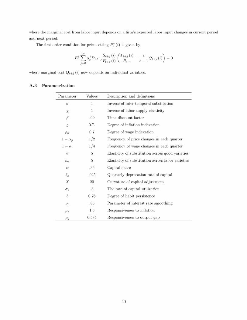
where the marginal cost from labor input depends on a firm’s expected labor input changes in current period
and next period.
The first-order condition for price-setting P ∗t (i) is given by
Ep̄t
∞∑j=0
αjpDt,t+jSt+j (i)
Pt+j (i)
(Pt+j (i)
Pt+j− ε
ε− 1Qt+j (i)
)= 0
where marginal cost Qt+j (i) now depends on individual variables.
A.3 Parametrization
Parameter Values Description and definitions
σ 1 Inverse of inter-temporal substitution
χ 1 Inverse of labor supply elasticity
β .99 Time discount factor
% 0.7. Degree of inflation indexation
%w 0.7 Degree of wage indexation
1− αp 1/2 Frequency of price changes in each quarter
1− αl 1/4 Frequency of wage changes in each quarter
θ 5 Elasticity of substitution across good varieties
εw 5 Elasticity of substitution across labor varieties
α .36 Capital share
δk .025 Quarterly deprecation rate of capital
X 20 Curvature of capital adjustment
σa .3 The rate of capital utilization
b 0.76 Degree of habit persistence
ρr .85 Parameter of interest rate smoothing
ρπ 1.5 Responsiveness to inflation
ρy 0.5/4 Responsiveness to output gap
40
Top Related