Introduction to variational autoencoders

Abstract Variational autoencoders are interesting generative models, which combine ideas from deep learning with statistical inference. They can be used to learn a low dimensional representation Z of high dimensional data X such as images (of e.g. faces). In contrast to standard auto encoders, X and Z are random variables. It’s therefore possible to sample X from the distribution P(X|Z), thus creating e.g. images of faces, MNIST Digits, or speech. In this talk I will in some detail describe the paper of Kingma and Welling. “Auto-Encoding Variational Bayes, International Conference on Learning Representations.” ICLR, 2014. arXiv:1312.6114 [stat.ML]. I will also show some code. A TensorFlow notebook can be found at: https://github.com/oduerr/dl_tutorial/blob/master/tensorflow/vae/vae_demo.ipynb

Introduction to variational autoencoders

Oliver Dürr Datalab-Lunch Seminar Series Winterthur, 11 May, 2016

2

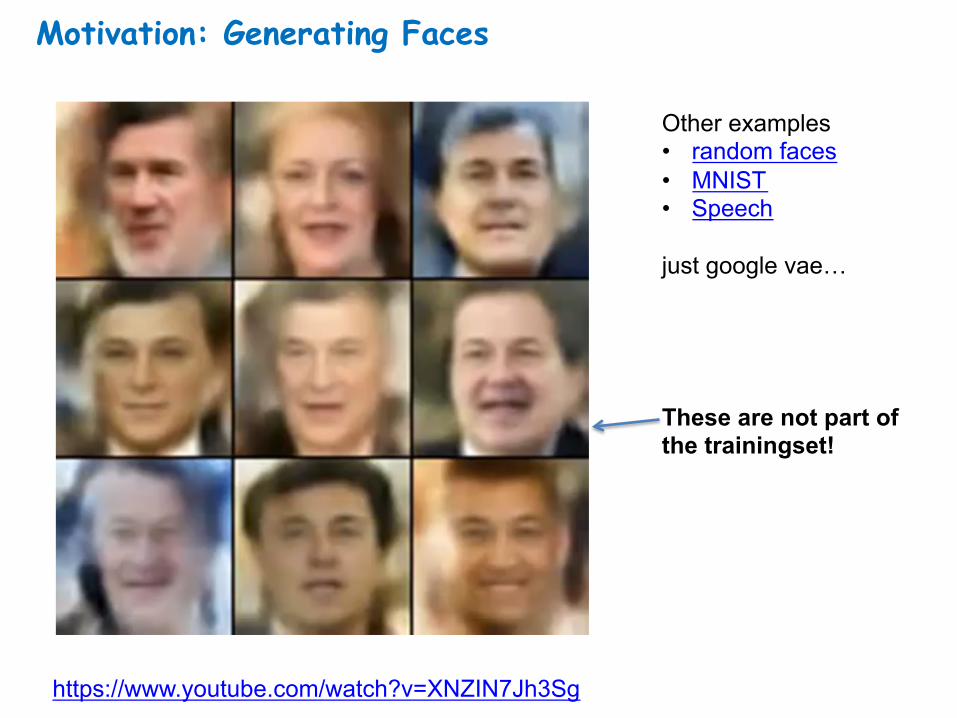
Motivation: Generating Faces

https://www.youtube.com/watch?v=XNZIN7Jh3Sg

Other examples •  random faces •  MNIST •  Speech just google vae…

These are not part of the trainingset!

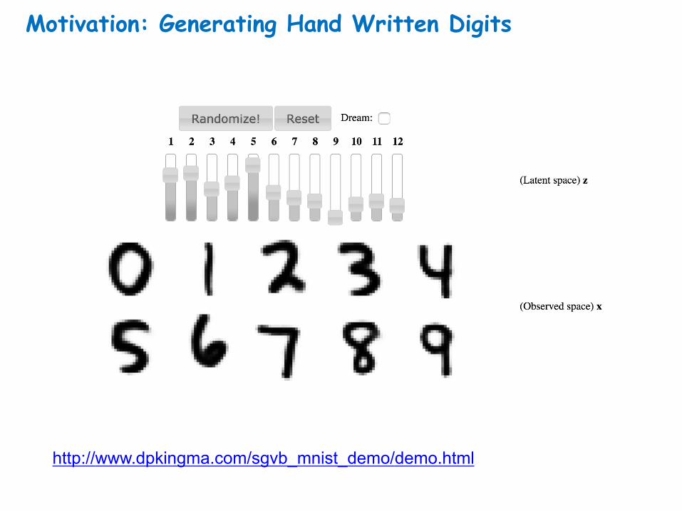
Motivation: Generating Hand Written Digits

http://www.dpkingma.com/sgvb_mnist_demo/demo.html

Idea

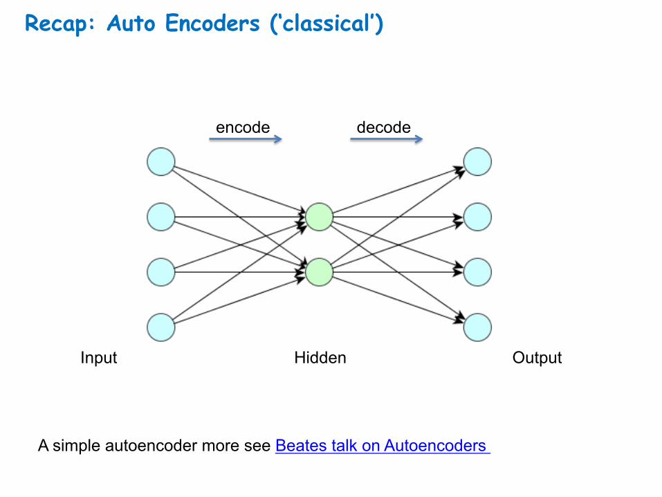
Recap: Auto Encoders (‘classical’)

A simple autoencoder more see Beates talk on Autoencoders

Input Output Hidden

encode decode

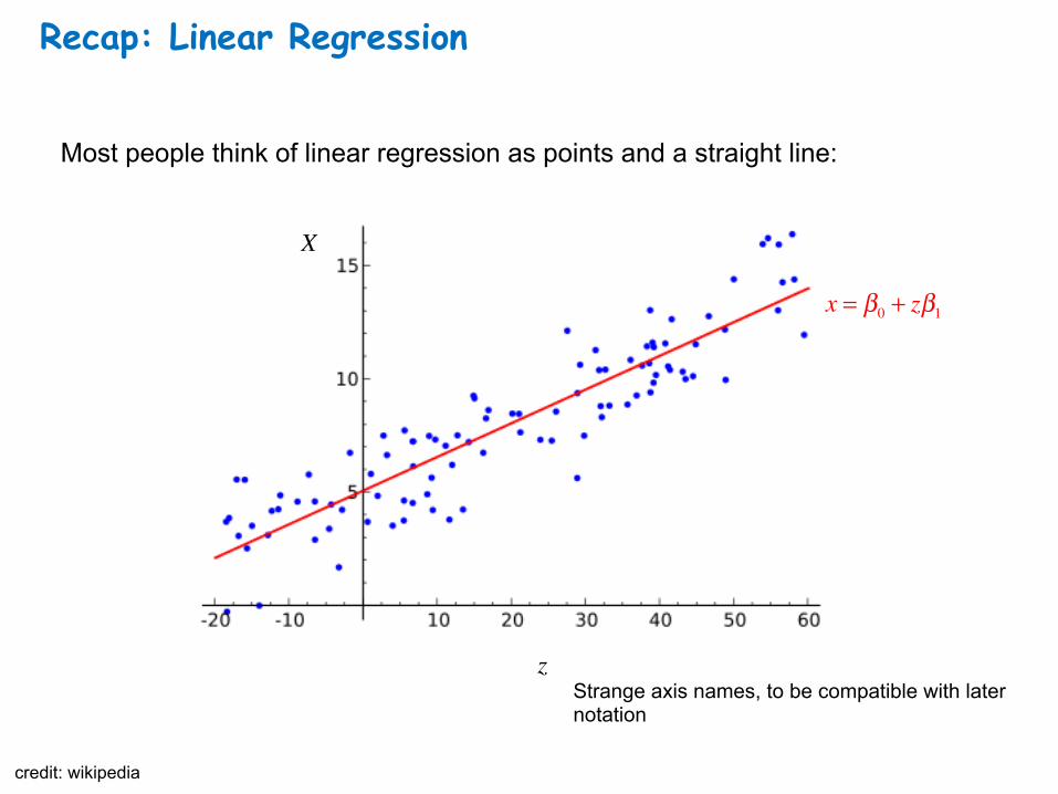
Recap: Linear Regression

Most people think of linear regression as points and a straight line:

Strange axis names, to be compatible with later notation

credit: wikipedia

x = β0 + zβ1

X

z

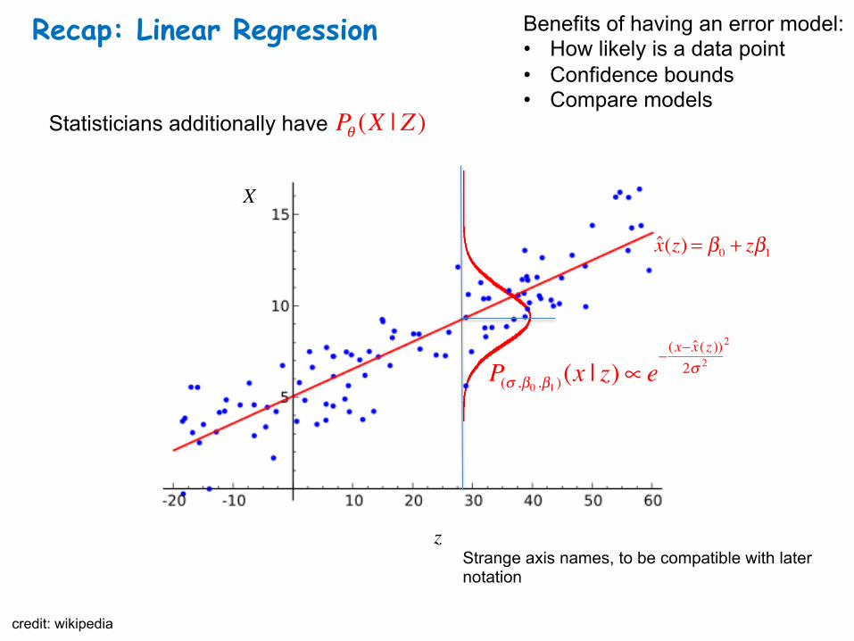
Recap: Linear Regression

Statisticians additionally have

Strange axis names, to be compatible with later notation

credit: wikipedia

Pθ (X | Z )

P(σ ,β0 ,β1 )(x | z)∝ e− (x− x̂(z ))

2σ 2

2

X

z

x̂(z) = β0 + zβ1

Benefits of having an error model: •  How likely is a data point •  Confidence bounds •  Compare models

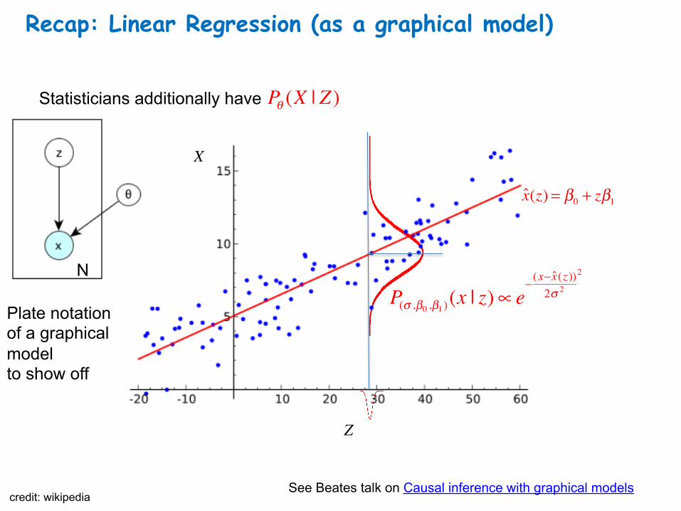
Recap: Linear Regression (as a graphical model)

Statisticians additionally have

credit: wikipedia

Pθ (X | Z )

P(σ ,β0 ,β1 )(x | z)∝ e− (x− x̂(z ))

2σ 2

2

X

Z

Plate notation of a graphical model to show off

x̂(z) = β0 + zβ1

N

See Beates talk on Causal inference with graphical models

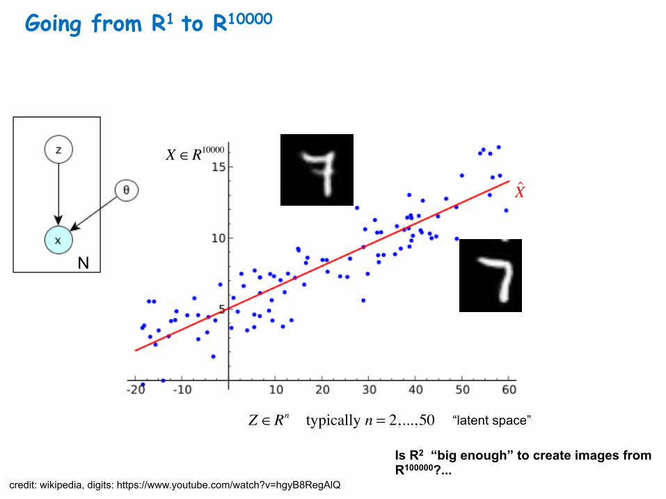
Going from R1 to R10000

credit: wikipedia, digits: https://www.youtube.com/watch?v=hgyB8RegAlQ

X̂

X ∈R10000

Z ∈Rn typically n = 2,...,50 “latent space”

Is R2 “big enough” to create images from R100000?...

N

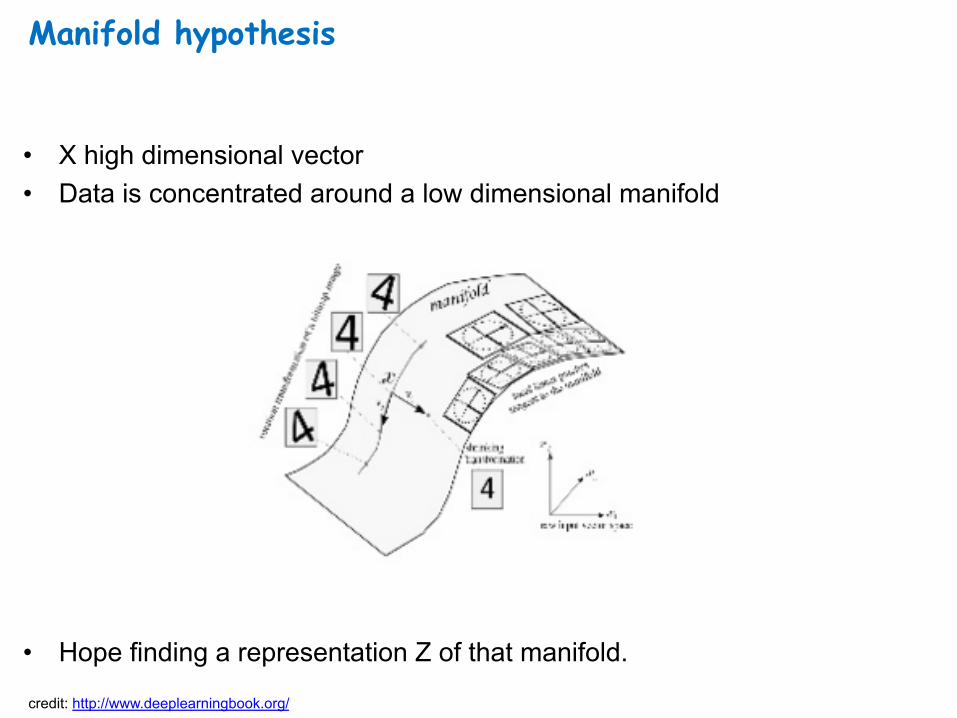
Manifold hypothesis

•  X high dimensional vector •  Data is concentrated around a low dimensional manifold

•  Hope finding a representation Z of that manifold.

credit: http://www.deeplearningbook.org/

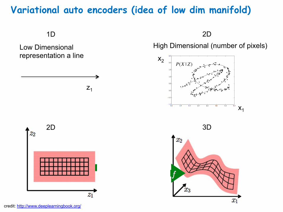
Variational auto encoders (idea of low dim manifold)

Low Dimensional representation a line

High Dimensional (number of pixels)

credit: http://www.deeplearningbook.org/

x1

x2

z1

P(X | Z )

1D 2D

2D 3D

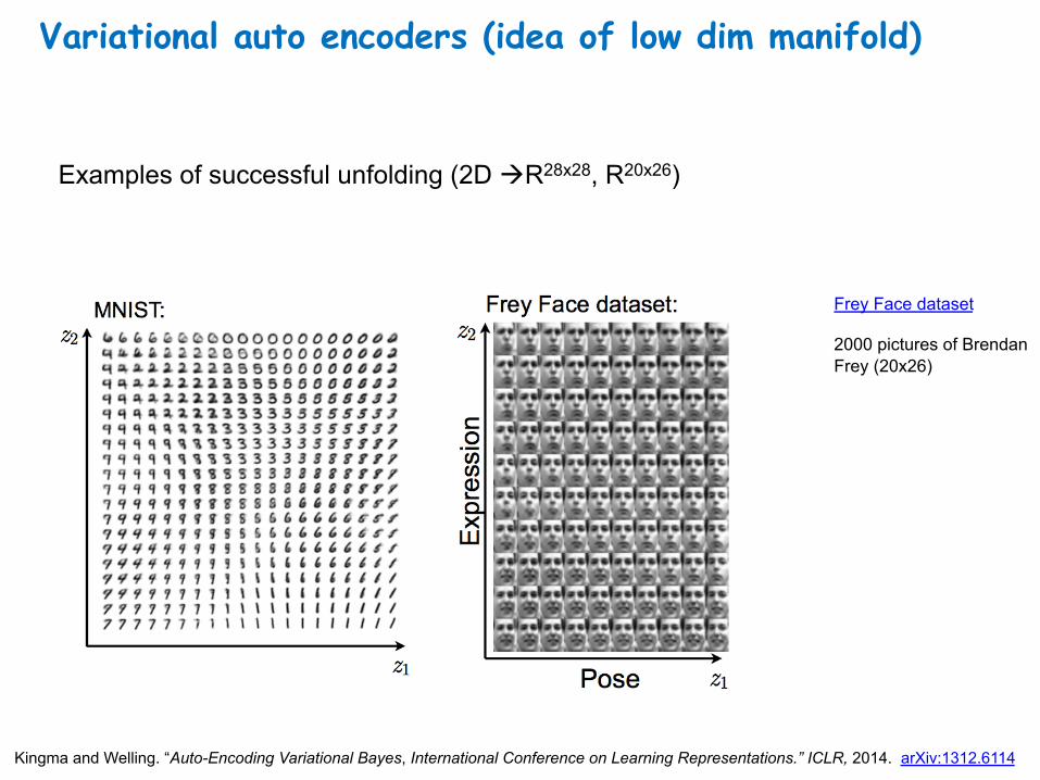
Variational auto encoders (idea of low dim manifold)

Kingma and Welling. “Auto-Encoding Variational Bayes, International Conference on Learning Representations.” ICLR, 2014. arXiv:1312.6114

Examples of successful unfolding (2D àR28x28, R20x26)

Frey Face dataset 2000 pictures of Brendan Frey (20x26)

How did they do that?

Variational Autoencoders (“history”)

Simultaneously discovered by •  Kingma and Welling. “Auto-Encoding Variational Bayes, International

Conference on Learning Representations.” ICLR, 2014. arXiv:1312.6114 [stat.ML] (20 December 2013, Amsterdam University) Talk

•  Rezende, Mohamed and Wierstra. “Stochastic back-propagation and

variational inference in deep latent Gaussian models.” ICML, 2014arXiv:1401.4082 [stat.ML] (16 January 2014, Google DeepMind)

Alternative approach (for binary distributions) •  Gregor, Danihelka et all. “Deep autoregressive networks.” ICML 2014

–  Has a more information theoretic ansatz (codings length) –  Lecture given at Nando de Freitas ML Course (University of Oxford) (a bit hand

waving argument but with nice examples)

•  We focus on the approach as in Kingma, Welling

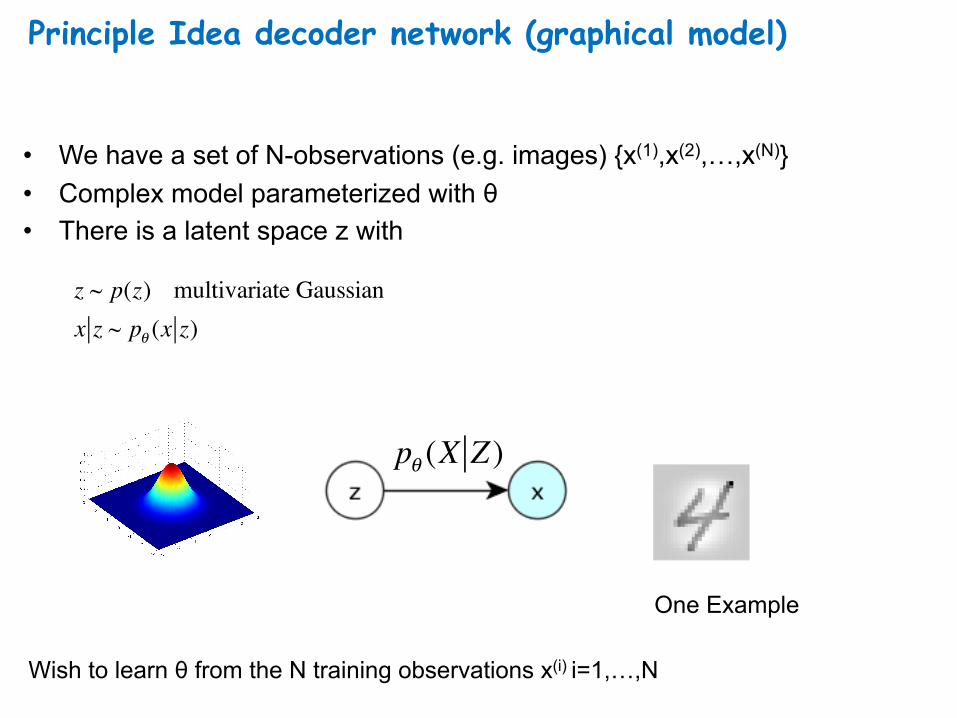
Principle Idea decoder network (graphical model)

•  We have a set of N-observations (e.g. images) {x(1),x(2),…,x(N)} •  Complex model parameterized with θ •  There is a latent space z with

z ~ p(z) multivariate Gaussianx z ~ pθ (x z)

Wish to learn θ from the N training observations x(i) i=1,…,N

One Example

pθ (X Z )

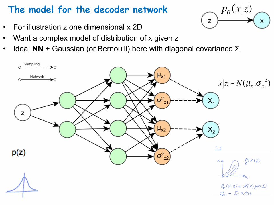
The model for the decoder network

•  For illustration z one dimensional x 2D •  Want a complex model of distribution of x given z •  Idea: NN + Gaussian (or Bernoulli) here with diagonal covariance Σ

pθ (x z)

µx1

σ2x1

σ2x2

µx2

X1

X2

x z ~ N(µx ,σ x2 )

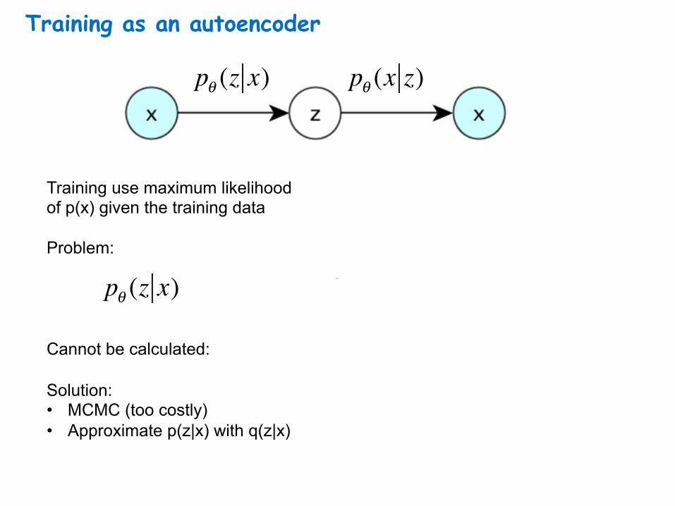
Training as an autoencoder

pθ (x z)pθ (z x)

Training use maximum likelihood of p(x) given the training data Problem: Cannot be calculated: Solution: •  MCMC (too costly) •  Approximate p(z|x) with q(z|x)

pθ (z x)

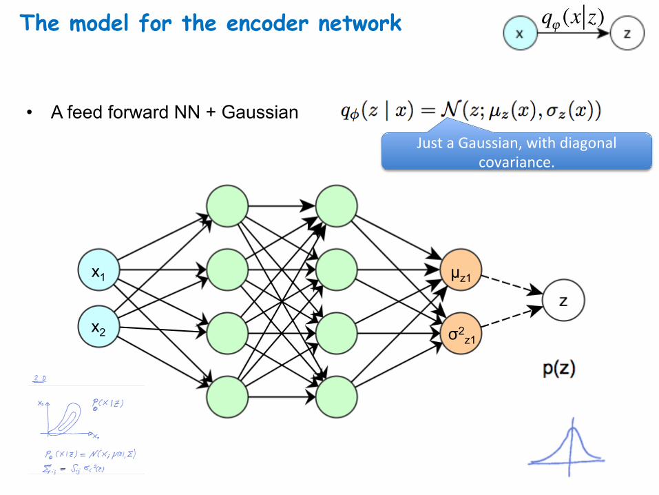
The model for the encoder network

•  A feed forward NN + Gaussian JustaGaussian,withdiagonal

covariance.

x1

x2

qϕ (x z)

µz1

σ2z1

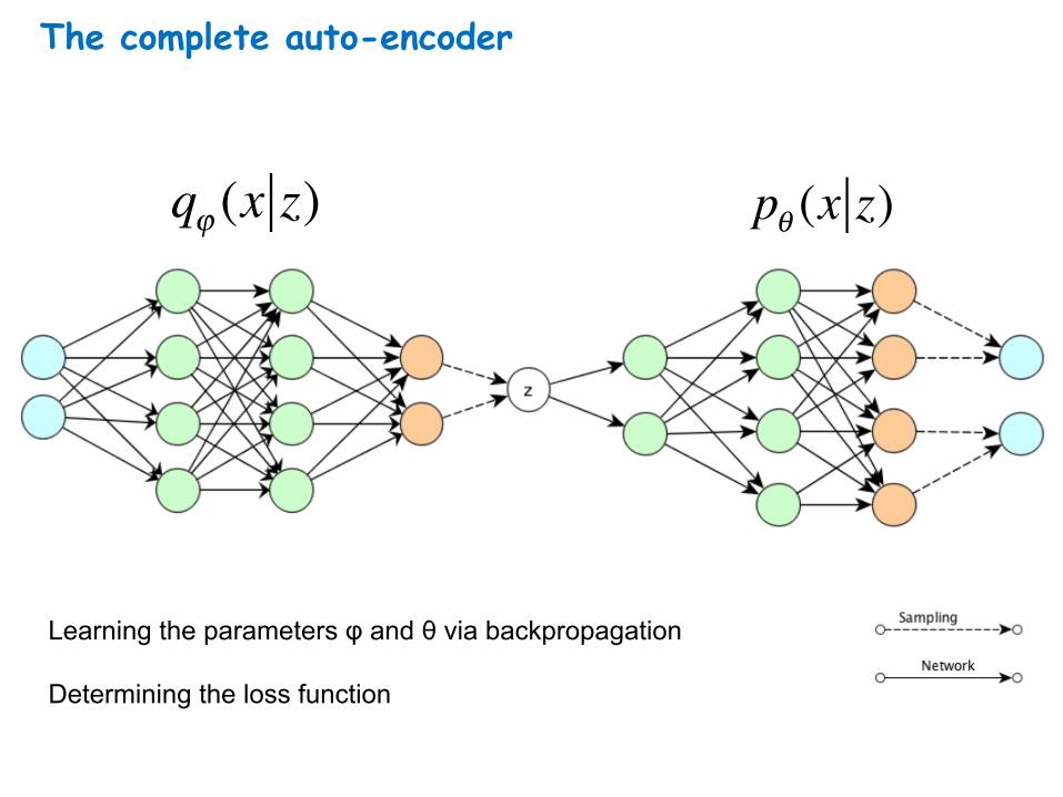
The complete auto-encoder

qϕ (x z) pθ (x z)

Learning the parameters φ and θ via backpropagation Determining the loss function

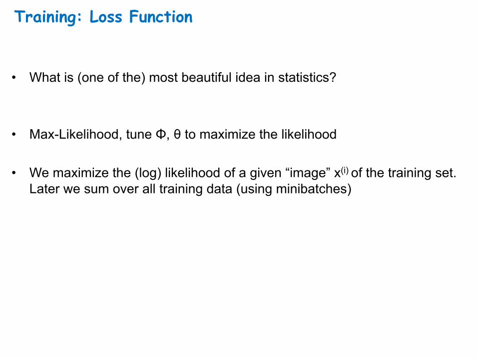
Training: Loss Function

•  What is (one of the) most beautiful idea in statistics?

•  Max-Likelihood, tune Φ, θ to maximize the likelihood •  We maximize the (log) likelihood of a given “image” x(i) of the training set.

Later we sum over all training data (using minibatches)

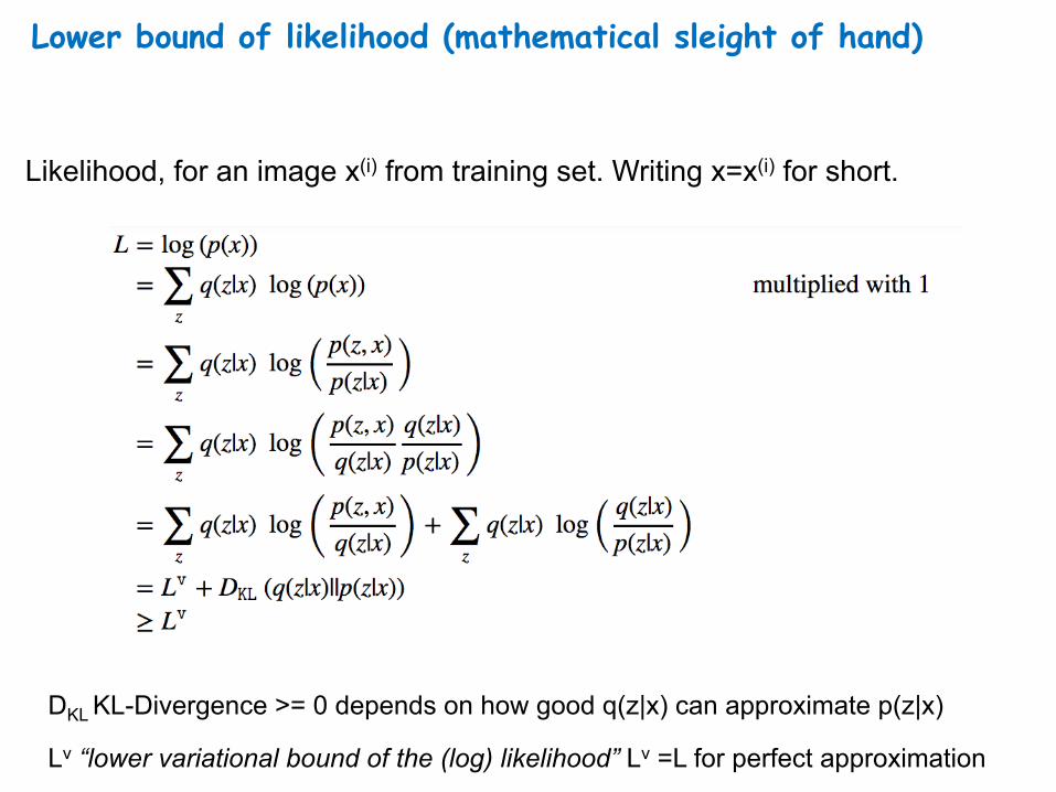
Lower bound of likelihood (mathematical sleight of hand)

Likelihood, for an image x(i) from training set. Writing x=x(i) for short.

DKL KL-Divergence >= 0 depends on how good q(z|x) can approximate p(z|x) Lv “lower variational bound of the (log) likelihood” Lv =L for perfect approximation

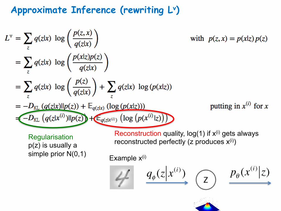
Approximate Inference (rewriting Lv)

pθ (x(i ) z)qφ (z x

(i ) )Example x(i)

Reconstruction quality, log(1) if x(i) gets always reconstructed perfectly (z produces x(i)) Regularisation

p(z) is usually a simple prior N(0,1)

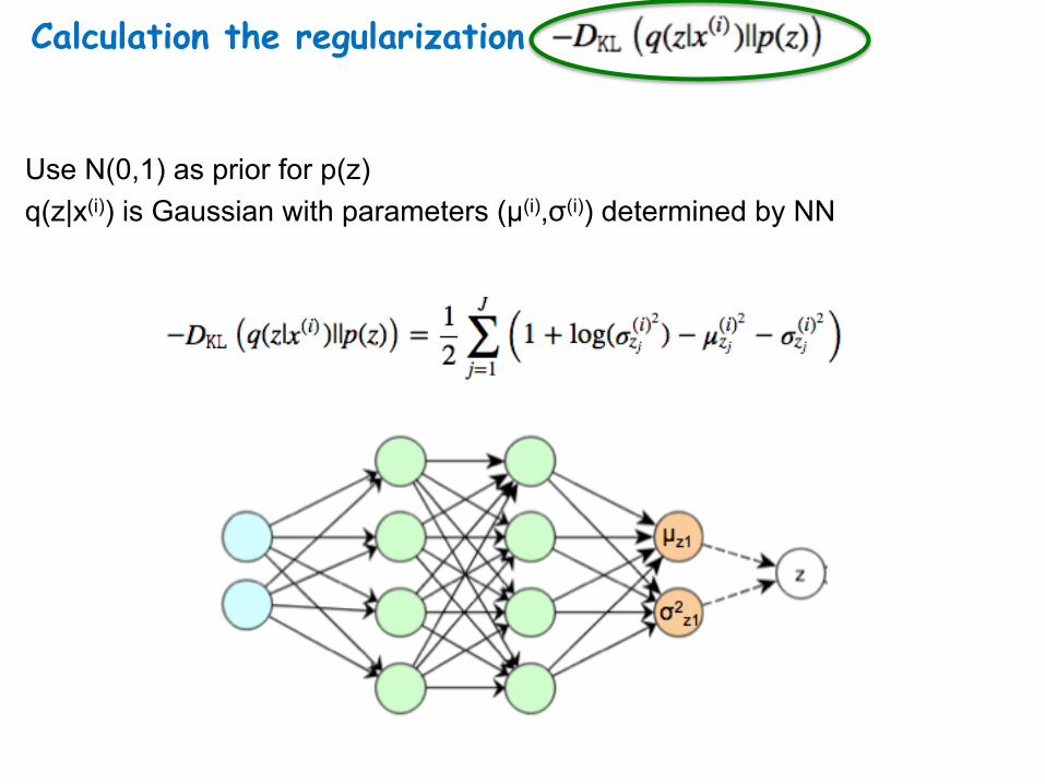
Calculation the regularization

Use N(0,1) as prior for p(z) q(z|x(i)) is Gaussian with parameters (µ(i),σ(i)) determined by NN

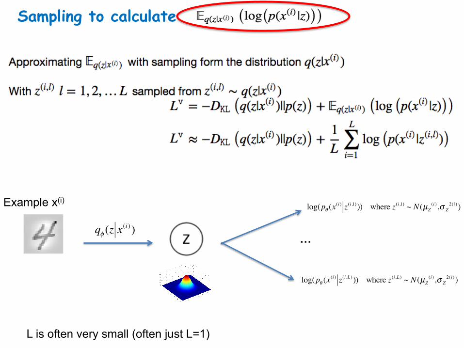
Sampling to calculate

log(pθ (x(i ) z(i,1) )) where z(i,1) ~ N(µZ

(i ),σ Z2(i ) )

qφ (z x(i ) )

…

Example x(i)

L is often very small (often just L=1)

log(pθ (x(i ) z(i,L ) )) where z(i,L ) ~ N(µZ

(i ),σ Z2(i ) )

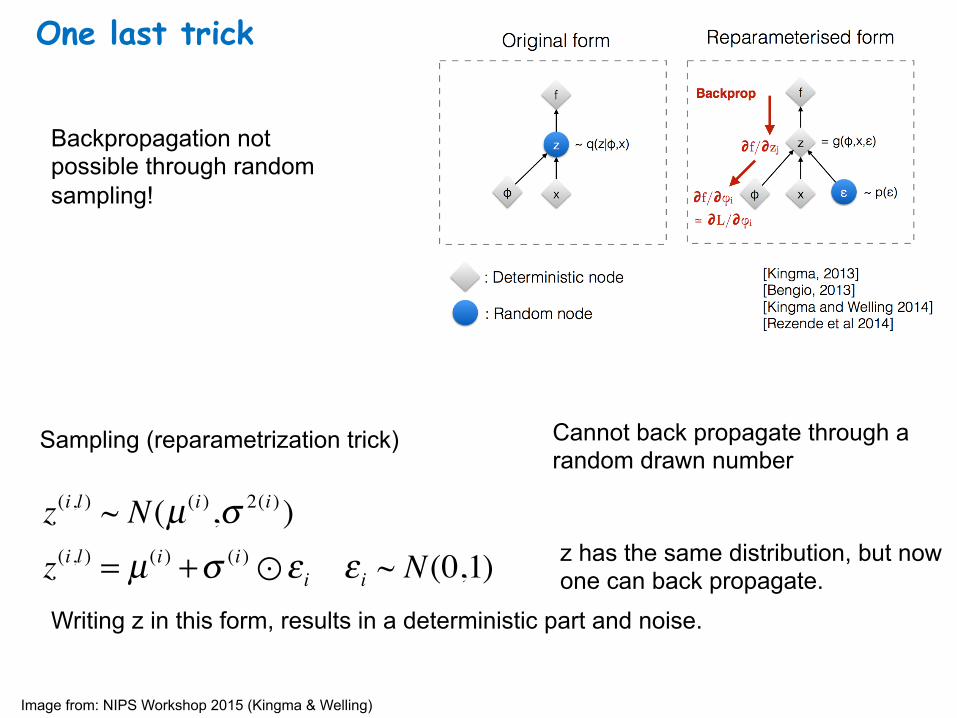
One last trick

z(i,l ) ~ N(µ (i ),σ 2(i ) )z(i,l ) = µ (i ) +σ (i )⊙ ε i ε i ~ N(0,1)

Sampling (reparametrization trick)

Writing z in this form, results in a deterministic part and noise.

Cannot back propagate through a random drawn number

z has the same distribution, but now one can back propagate.

Backpropagation not possible through random sampling!

Image from: NIPS Workshop 2015 (Kingma & Welling)

Putting it all together

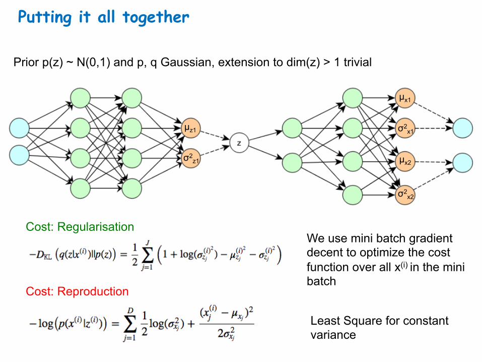
Prior p(z) ~ N(0,1) and p, q Gaussian, extension to dim(z) > 1 trivial

Cost: Reproduction

Cost: Regularisation We use mini batch gradient decent to optimize the cost function over all x(i) in the mini batch

µx1

σ2x1

σ2x2

µx2

µz1

σ2z1

Least Square for constant variance

Use the source Luke Simple example 2-D distribution https://github.com/oduerr/dl_tutorial/blob/master/tensorflow/vae/vae_demo-2D.ipynb

Simple MNIST Example https://github.com/oduerr/dl_tutorial/blob/master/tensorflow/vae/vae_demo.ipynb

Recent developments of VAE

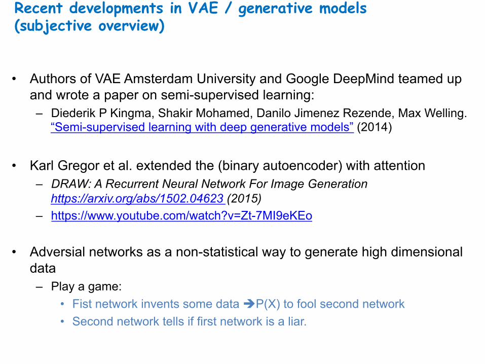
Recent developments in VAE / generative models (subjective overview)

•  Authors of VAE Amsterdam University and Google DeepMind teamed up and wrote a paper on semi-supervised learning: –  Diederik P Kingma, Shakir Mohamed, Danilo Jimenez Rezende, Max Welling.

“Semi-supervised learning with deep generative models” (2014)

•  Karl Gregor et al. extended the (binary autoencoder) with attention –  DRAW: A Recurrent Neural Network For Image Generation

https://arxiv.org/abs/1502.04623 (2015) –  https://www.youtube.com/watch?v=Zt-7MI9eKEo

•  Adversial networks as a non-statistical way to generate high dimensional data –  Play a game:

•  Fist network invents some data èP(X) to fool second network •  Second network tells if first network is a liar.

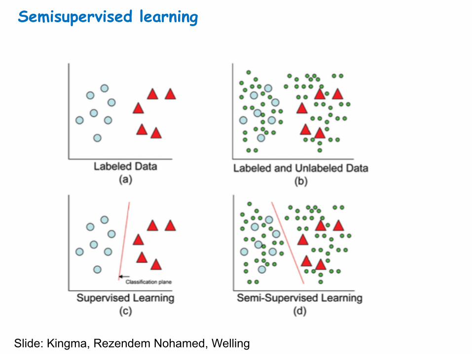
Semisupervised learning

Slide: Kingma, Rezendem Nohamed, Welling

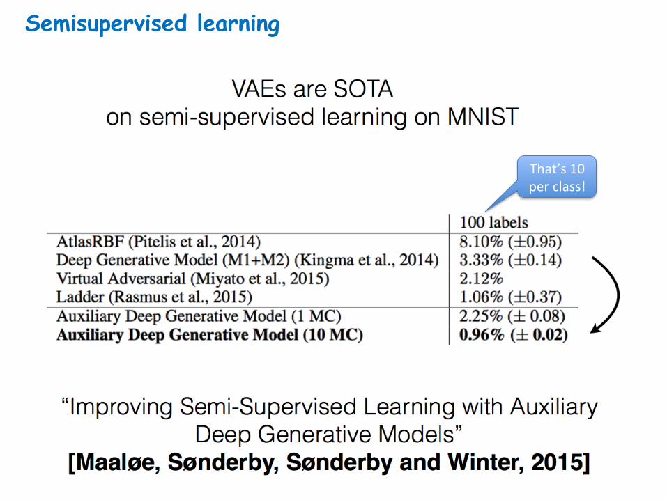
Semisupervised learning

That’s10perclass!

Thank you, questions?