


Languages
Pages
Legal


Introduction to the Design of Mobile Hydraulic Systems - Part 1 Course No: M02-044
Credit: 2 PDH
K. Michael Clark, P.E.
Continuing Education and Development, Inc. 9 Greyridge Farm Court Stony Point, NY 10980 P: (877) 322-5800 F: (877) 322-4774 [email protected]

INTRODUCTION
In writing this review course the reader is envisioned as the practicing engineer who has been given the task of designing a hydraulic system for a new piece of mobile equipment. It is assumed that the engineer has a good foundation in general engineering principles and simply needs a brush‐up on applied fluid flow principles and an introduction to the unique considerations of hydraulic control systems. Equations required for analysis are presented, but not derived. The review is divided into two courses, with this being Part 1.
The reason hydraulics is selected for most mobile applications is that hydraulics have the highest power density available to the designer. This includes the highest power per pound or per cubic inch. This is especially true if the vehicle already has a prime mover (diesel engine) with a PTO (Power Take Off) on the transmission. The down side of hydraulics is that hydraulics is potentially a messy system. When a hydraulic system leaks, it is obvious to everybody.
The design of many systems will not need the entire course. For example many systems operate very intermittently with short ‘on’ periods separated by long ‘off’ periods. This type of system often does not require active heat exchange to maintain acceptable fluid temperature. In addition, some systems are able to use large vented reservoirs and the reservoir has sufficient surface area to cool the fluid even on the hottest day. However, it is suggested that at least a cursory review of the heat balance be made in the design phase. It is much easier to correct a problem during design than fixing an existing system. Eraser dust cost less than metal chips.
Reviewing Hydraulic fundamentals in a static control volume (no flow) the pressure is the same everywhere in the system or container. The shape of a container does not affect the pressure. Region 1 below may be the discharge port of a pump, Region 2 could be a tube or hose between components, and Region 3 may be in a cylinder or motor piston. With no flow there will be no pressure losses (losses are discussed later in the course), so the pressure is constant throughout.

The effects of variation in elevation on pressure are normally neglected. A few percent change in pressure due to static head will make no difference in the operation of most systems. The exceptions to this are systems with large variations in vertical elevation like oil wells or tall refinery towers. In the design of your system, you must decide if elevation can be neglected. In case you need it, the figure below describes the calculation of pressure due to vertical elevation.
• Consider a 1 cubic foot cube of fresh water sitting on a scale. The weight of 62.4 Lbs. is distributed over 1 square foot, or 144 square inches.
• The pressure supporting this 1 foot column is: 62.4*SpGr/144 = 0.433*SpGr psi/foot, where SpGr is the specific gravity of a general liquid.
• In a 100 foot column of water, this is 43 psi and is significant for a 500 psi system, negligible in a 3000 psi system.
In a hydraulic system the conservation of material or continuity is strictly observed. The fluid is generally treated as incompressible. If a volume of fluid flows into a control volume, it either must flow out another port, or the control volume must expand (extend a cylinder for example) at the same rate.
Similarly, energy is also conserved in a hydraulic system. If power is put into a system by a pump, that energy is evidenced as the pressure of the fluid. In a flowing system, the relationship between potential energy (static pressure), kinetic energy (dynamic pressure) and total energy (total pressure) is described by the Bernoulli equation and will be used in the second course in analysis of pressure loss in a system.
In the design of a system there inevitably are several things that have to be done “first.” When faced with this type of situation, define on a preliminary basis, the necessary parameters. This recognizes that the design process is an iterative process. The first time through will require some assumptions. Write the assumptions down and resolve or verify them later by analysis. One early task is to define the loads to be moved by the hydraulic system (load vs. stroke or time for a cylinder, or torque vs. time for a motor). The implication is that you know the time lines for each function the hydraulic system is to accomplish. If your system will be manually controlled with ‘eyes on the load’ you still have a range of acceptable speeds of the load. Regardless, it is a good idea to write down all assumptions made subject to later review.
The system of symbolic representation used in this course is found in SAE AS‐1290 “Graphical Symbols for Aircraft Hydraulic and Pneumatic Systems.” A web search of ‘hydraulic symbols’ will provide a number of sites defining these symbols such as:
www.me.ua.edu/me360/fall05/Misc/Hydraulic%20Schematic%20Symbols.pdf
In the chemical process industry, an alternate system of symbols is used to develop Process and Instrumentation Design (P&ID). This system includes a lot of additional symbols for devices not necessary in typical mobile hydraulic systems. A web search on P&ID will yield a number of sites defining this system. The engineer is responsible for selecting the correct system for the application. Often the customer will have a preferred system of symbols.
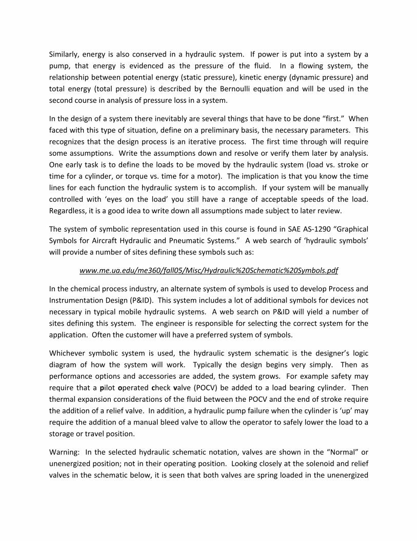
Whichever symbolic system is used, the hydraulic system schematic is the designer’s logic diagram of how the system will work. Typically the design begins very simply. Then as performance options and accessories are added, the system grows. For example safety may require that a pilot operated check valve (POCV) be added to a load bearing cylinder. Then thermal expansion considerations of the fluid between the POCV and the end of stroke require the addition of a relief valve. In addition, a hydraulic pump failure when the cylinder is ‘up’ may require the addition of a manual bleed valve to allow the operator to safely lower the load to a storage or travel position.
Warning: In the selected hydraulic schematic notation, valves are shown in the “Normal” or unenergized position; not in their operating position. Looking closely at the solenoid and relief valves in the schematic below, it is seen that both valves are spring loaded in the unenergized

position. Many electrical designers interpret “Normal” to mean the “normal operating position.” Be sure the electrical designer is aware of this convention.
A notional system schematic is shown below.
A few words on system design approach are necessary. A control system should be designed to always have absolute control of the loads. From a safety standpoint, you can never lose authority over a load. In a feed‐back control system you want absolute control to repeatedly dispense the smallest packet of fluid, and that packet of fluid must have absolute authority over the load to make the smallest possible movement or correction.
It is important to understand that hydraulics “push, not pull.” A motor or cylinder may be driven by a 3000 psi differential pressure across it (i.e. the fluid is “pushing” the load). The equations defining the force and performance are given later in this course. If the hydraulics try to “pull” the load, vacuum only goes to negative 14 psi gage (zero absolute pressure). In fact, the pressure on the vacuum side will not even go that low. The hydraulic fluid will vaporize and fill the volume once the pressure reduces to the fluid vapor pressure. If the designer relies on vacuum, they will lose control of the load. In a 3000 psi system, vacuum side load capability is only 14/3000 or 0.5% of the pressure side load capability.
In sizing a pump or motor, an early decision is the system pressure. If this is not given (by past experience, or requirement) it is suggested that the system be sized for two pressures. To accomplish the same work, higher pressure systems require lower flow rates and smaller devices. Typically end devices are available from catalogs for 2000 psi, 3000 psi, and 5000 psi pressure rating. Only a few devices rated for 5000 psi are available in published catalogs. If higher pressures are needed, work closely with the vendor to develop devices.

Size all load moving end devices first. For several loads moving simultaneously, the several flow rates have to be summed up to determine the pump delivery rate required. Care must be taken in summing several non‐linear flow rates that the maximum flow rate is identified. Pump delivery is a function of the pump displacement (cubic inch per revolution or CIR) and the pump speed (rpm). If peak flow rate is required only for a few seconds, possibly that peak demand may be satisfied by an accumulator instead of a larger pump.
When designing the system, there are two ways to control system pressure. The easiest to understand is a system where the pressure is controlled by a variable displacement pump (#10 in the notional schematic above) or a relief valve (#29 above). The maximum flow rate required by the system is slightly less that the max delivery rate of the pump and the system pressure is determined by the pump pressure compensator or system relief valve.
The second way to control system pressure is when the load uses all the flow from the pump. In this case the system pressure is determined by the pressure required by the load. This system will still require a pressure relief valve to prevent over‐pressure at each end of the required movement of the load, or to limit maximum load in the event of an unforeseen problem. This type of system usually utilizes manual control valves with “Open Center”, which means that in the neutral position, the pump port is directed to the reservoir. If multiple loads are designed to move at the same time, the load with the lowest ∆P requirement will move first, followed by the next lowest, etc.
With the pump and end devices defined, the flow rates are defined. Now determine preliminary hose and tube sizes. As a goal, keep the fluid velocity below 10 feet per second to manage pressure loss. Valves, filters, and other accessories should be collected in a manifold to simplify the system and reduce opportunities for leaks. For widely distributed systems several distributed manifolds may be required. Now fit everything into the vehicle. Make the changes necessary and analyze until it fits and works.

END DEVICES
End Devices are the cylinders, motors, and pumps that actually convert pressure energy and power into motion (cylinders and motors) or convert mechanical energy into pressure energy (pumps). To this list, I have added reservoirs and their sizing will be discussed last in this section.
Cylinders
The simplest end device is a cylinder. Shown below is a single stage double acting cylinder. Double acting means that the cylinder is capable of force in either extend or retract direction. Illustrated below is the extend direction.
Cylinder Performance Analysis
Force = (PH) (AH) – PR (AH – AR)
FlowHead = π(DH/2)2 *(Rod Vel) / 231 gpm
FlowRod = π((DH/2)2 – (DR/2)2 )* (Rod Vel) / 231 gpm
Where
P ~ Lb/in2
A and D ~ inch2 and inch
Rod Vel ~ inch/minute

Retract direction of force is achieved by reversing the direction of flow. The servo‐valve from the example system schematic earlier is shown on the right below. The switch in ports is achieved with a manual or servo 4‐way control valve like this. On one end of the valve the lines are connected straight through.
On the other end they are crossed which reverses the pressure and tank locations on the end device. If the cylinder is load bearing, you must do something to maintain control. Possibly a pilot operated check valve or some type of flow rate control will work. (This will be discussed later in the course).
Shown below is a single acting two stage cylinder that might be used for a longer reach where the load is always compressing the cylinder. To use a single acting cylinder it is very important that the direction of force is always compressing the cylinder and it never reverses, even momentarily due to unplanned occurrences. It is very important to understand that “hydraulics push loads, they do not pull or suck loads.” If the cylinder below is placed in tension it will uncontrollably extend to the stops. The pressure in the head end will reduce to the fluid vapor pressure and boil to fill the volume with vapor. Staged cylinders may be any number of stages, limited only by mechanical design considerations and cylinder stability. Three and four stage cylinders are common. The first stage to extend (and last to collapse) is the largest diameter, followed by the next smaller, etc. and last will be the smallest diameter stage. The smallest diameter stage will be the first to collapse. In a single acting cylinder, the control valve only needs to switch the single line between pressure, off, and tank. The un‐pressurized side of most single action cylinders is usually vented.

To size a cylinder one needs to know the force and stroke required by the load, and if force is required in both directions (double acting) or only one. Size the cylinder diameter to give the required force plus a few percent margin. Be sure to allow for pressure losses under the worst operating condition (cold). Next, determine the speed the cylinder must move to give the desired or required speed of the load and calculate the flow rates (both ends for double acting) required. As with force, it is wise to carry a few percent margin forward to size the pump later.
Motors and Pumps
The next step up is a motor or pump. Conceptually pumps and motors differ only in the direction that energy or power is flowing. Shown below is a schematic of a gear pump. Torque is input via the shaft to one of the gears rotating both gears. Fluid moves around each gear in the cavity between the teeth from the suction side to discharge. If this sketch was a motor, the port labeled ‘Suction’ would be ‘Pressure’; ‘Discharge’ would be labeled ‘Tank’; and torque would be removed via the shaft. In both pumps and motors there are no valves limiting flow in either direction. If you want to lock the load in place with the motor, you will have to use a closed center valve that shuts ‘off’ one or both lines to the motor, a pilot operated check valve, a brake, or some other way to lock the load.

http://en.wikipedia.org/wiki/File:Gear_pump.png
An exploded view of a typical gear pump is shown below. This figure is from a Parker catalog as indicated. Typically a gear pump or motor is the lowest purchase price high pressure device available. However, they have higher maintenance costs and are unsuitable for systems with servo‐valves in them because of their higher solid particle generation rate. Usually gear pumps are heavier than other pumps and motors of the same performance caliber.

At the high end of cost and reliability and low end of weight is the pressure compensated piston pump or piston motor. Typically the pressure compensated pump is an ‘in‐line’ configuration as shown below with a variable yoke to change pump displacement from near zero up to design maximum displacement in response to discharge pressure or other options.
Eaton Vickers Fluid Systems: “Descriptive Summary of Vickers Inline Pumps and their Applications”
Pressure compensated piston pumps are substantially more expensive than gear pumps. Also, piston pumps generally require much higher pump suction pressure (NPSH). Often a pressurized reservoir is used. On the advantage side, piston pumps and motors properly applied will have much lower failure rates and over the long run, lower total cost when the costs of down time and maintenance are included.
Motors usually are ‘bent axis’ configuration with fixed displacement per revolution. Piston pumps and motors are suggested for systems that include servo‐valves or proportional valves because of the relatively low rate of particle generation by piston devices. Servo‐valves are very sensitive to fouling and damage from solid particles in the fluid.
The equations describing the performance of rotating hydraulic motors and pumps are seen below. When sizing the motor, be sure the motor is capable of about 10 percent more torque (at the selected ∆P) than the maximum required by the load. If the motor cannot provide the required torque it will not start, or when torque required exceeds motor torque available the motor will stall. With the motor sized, then calculate the flow rate to total with other load flows to size the pump.

Pumps and Motors (American Standard Units)
Torque = CIR * ∆P / 2π in‐lb
Flow Rate = CIR * rpm / 231 gpm
Shaft Power = Torque * rpm / 63025 hp
Hydraulic Power = gpm * ∆P / 1714 hp or hhp
Where:
CIR = pump or motor displacement cubic inch/revolution
gpm = gallons / minute
∆P = pounds / inch2
Pumps amd Motors (Metric Units)
Torque = (mL/rev) * ∆bar / (20π) N‐m
Flow Rate = (mL/rev) * rpm / 1000 L/min
Shaft Power = W = π * Torque * rpm / 30 watts
Hydraulic Power = (5/3) * (L/min) * ∆bar watts
Where:
mL/rev = pump or motor displacement, mili‐Liter/rev.
KPa/1000 may used in place of bar

Reservoir
In the industry the term ‘reservoir’ and ‘tank’ are used interchangeably. The reservoir is not a typical ‘End Device’; however, in a system that must limit reservoir volume, it’s sizing requires consideration. The reservoir must satisfy several system requirements such as providing volume for thermal expansion of the hydraulic fluid, differences in fluid volume out in the system (a cylinder extended vs. collapsed), make‐up volume for minor routine system leaks between normal servicing, and maybe cooling of the fluid. Coefficient of thermal expansion of typical hydraulic fluids is about 0.0008/°C. If the difference between cold and maximum operating temperature is 200°F or 111°C, this will result in about 8% expansion of the fluid volume. In a 10‐gallon system, the expansion will be about 0.8 gallons. If you don’t have room for this additional gallon of fluid, it will end up on the ground, or maybe when cold, you will not have enough fluid to fully extend the cylinder.
Plumbing Components
Reservoirs, pumps, motors, etc. are of no value without suitable plumbing between the devices, valves and manifolds. Several words of advice and caution are necessary.
In an ideal world the plumbing components would be designed using CAD software. However, often the model of the host vehicle is not sufficiently accurate to design the routing and plumbing details. Many times hydraulic plumbing components have to be routed in the ‘unused corners’ of a vehicle frame or chassis to get from one end of the vehicle to the other. CAD models usually do not detail these corners, and often electrical and pneumatic routing in these corners is not in the models. If an accurate and detailed model of the vehicle is available, you may be able to use it subject to the following cautions.
Hydraulic plumbing often includes what is called ‘clocking’ of the end fittings. Clocking is the orientation of an angled end fitting relative to the orientation of the angled end fitting on the other end of the hose. As of 2010, I do not know of a CAD package that will satisfactorily keep track of clocking of hydraulic hoses. If your hoses can include one straight end, CAD will work fine. Often this is possible by including or installing an angled fitting with ‘swivel nut’ installed on a straight union on one end (end device, manifold, or junction block).
CAD does a better (but still not perfect) job of keeping track of clocking of steel tubing. When designing steel tubing you also have to keep track of the clocking of bends throughout the length of the tube. My suggestion is to minimize joints (potential leaks), however the steel tube has to be able to be snaked into the vehicle. Also consideration has to be given to how a joint between two plumbing components or end device is going to be made. If you cannot get to a junction with a wrench, there are ‘snap connections’ available from several vendors. However, these have to be verified ‘made’ and occasionally separated for maintenance.

An alternative to designing plumbing with CAD is to mock‐up plumbing components with plastic pipe. Slip‐assemble each component in the vehicle, mark each elbow sequence, orientation, clocking, and decide where junctions will be. Remove and make sure identification is adequate for your vendor to re‐assemble and ship off to your hose and tube vendor for fabrication. The very real down‐side of ‘mock‐up design’ is that at least one major hose and tube vendor will not work with you this way. Additionally, if you work for a large company, your receiving department may not release vendor hardware for check‐fit and installation without a company drawing for them to verify the accuracy of the component. Do not go around your receiving department when receiving check‐fit or initial installation hardware. Their accounting of received hardware is essential to ensure accurate payment for hardware. Before you begin down the mock‐up design path, be sure everyone is on board.
If your system is in a high vibration environment, you have to address the support and restraint of the plumbing components. Vendors of hydraulic components have guidelines for support. Components near an engine or installed on a tracked vehicle require support and restraint to prevent premature failure due to the vibration.
There are dozens of styles for tube and hose end fittings. These are described in SAE‐J514, SAE‐J1926, SAE‐J1453, and others (and these are just a few threaded fittings). Stated another way, there are ‘O‐ring boss,’ ’O‐ring face seal,’ ’37 degree,’ ‘flareless,’ pipe, as well as several other high pressure fittings. In addition, there is another wide selection of metric fittings and adaptors. Many times a company will have a history and preference for one style of fitting. Each style has its advantages and limitations. You need to pick a fitting style and system pressure together because some fitting styles are rated for higher pressure than others. Pipe fittings when properly applied will work fine. However, after repeated ‘break’ and ‘make’ cycles, pipe will make up shorter in overall length, and will clock differently making it difficult to work with.
Pressure ratings of several popular fitting styles are shown in the following table for reference. It is advisable to verify these pressure ratings in the current issue of the referenced specifications when beginning a new project.

WORKING PRESSURE RATINGS
OF
SEVERAL POPULAR FITTING STYLES
SAE Dash No.
Nom. Tube Size Inch
SAE Straight Thread ORB and 37° Blkhds.
SAE Straight Thread Adjustable Unions, Bkh
SAE Straight Thread O‐Ring Face Seal
Nom. Pipe Size Inch
Pipe Fittings
‐02 0.125 5000 psi 5000 psi 1/8 5000 psi ‐04 0.250 5000 4500 6000 psi ¼ 5000 ‐06 0.375 5000 4000 6000 3/8 4000 ‐08 0.500 4500 4000 6000 ½ 3000 ‐10 0.625 3500 3000 6000 5/8 3000 ‐12 0.750 3500 3000 6000 ¾ 2500 ‐16 1.000 3000 2500 6000 1 inch 2000 ‐20 1.25 2500 2000 4000 1 ¼ 1150 ‐24 1.5 2000 1500 4000 1.5 1000 ‐32 2.00 1500 1125 2 inch 1000 Ref:
SAE‐J‐514 for ORB, 37° Flare and Pipe data (Table 1)
SAE‐J‐1453 for O‐Ring face seal data (Table 4)

HYDRAULIC CONTROL SYSTEM VALVES
Valves are the directors or brains of the hydraulic system. End devices are the muscle of the system. Most mobile hydraulic control systems use an assortment of ball‐and‐seat (or thimble and seat), and spool valves to control and direct fluid to the load or end device desired. In a manual control system, these valves will be manually controlled by a handle. The manual handle may actually move the control valve, or it may move a pilot valve that directs pressure to one end or the other of the actual control valve, or the handle may switch an electrical signal that directs electrical power to move the hydraulic valve or pilot valve. Other valves are actuated by pressure. Pressure actuated valves include pressure relief or pressure regulator valves, pilot operated check valves, or constant volume valves. The design of hydraulic valves is another subject and not included in this course. Spool valves may simply turn a single tube of fluid on or off in a ‘two‐way‐valve’ (#23 and #29 in notional schematic), or may switch both power and return in a ‘four‐way‐valve’ (#22). Valve vendors include Canyon Engineering, Crissair, Kepner, Lee Company, Moog, Parker, Sun Hydraulics, Circle Seal, Ausco, and many others. Links to these vendors are included in the ‘Resources’ portion of this course.
Valves come in an amazing variety of functions. Illustrated above are two variations. The first illustration shows a 3‐position 4‐way valve with the pressure and return ports routed together in the neutral position that might be used in a single function system to unload the pump when the system is idle, thereby, reducing the heat generation and prime mover fuel consumption. The second illustration shows a 2‐position 4‐way valve with the load A and B ports routed together and to Tank in the OFF position that might be used to unload the end device when idle. The point is, if you need a valve configuration and do not see it in a catalog, ask the vendors if such a valve can be made for you. It is likely that you are not the first to request that valve and they probably have an existing design and can build what you need.
Valve manufacturers produce valves in various sizes. Vendors provide flow characteristics in terms of pressure drop vs. flow rate or in terms of Cv for each size for water flowing through the valve. Various units are used so be careful to use or convert the data into the units you are using. For general analysis, valve pressure drop is a dynamic loss and is only a weak function of fluid viscosity. Viscosity is usually neglected when calculating valve pressure drop.
In addition to manual or electrically actuated valves, there are pressure actuated valves used for pressure relief (#29) or pressure regulation applications. Pressure relief or pressure regulation valves usually are either fully closed or fully open. Also there usually is a small pressure window between the opening pressure and closing pressure. Depending on your
application, some care must be exercised to properly size these valves. Using too large a valve will result in the valve rapidly ‘chattering’ open and shut. Too small a valve will not relieve enough flow to keep maximum pressure within the desired limits.
Pressure relief and pressure regulation differ schematically only in which side of the valve the pressure sensing port is on. If the pressure sensing port is on the down‐stream, or load side, of the valve the pressure to the load will be regulated or prevented from exceeding some value. This might be used to limit maximum force or torque at an end device.
In the simple schematic used throughout this course, a simple relief valve (#29) is shown in addition to a pressure compensated pump. In this case, the relief valve is optional and should contain damage from failure of the pump pressure compensation to the pump only. Also in this schematic, a simple ‘2‐way’ solenoid valve is shown (#23) to pressurize a sub‐manifold for other functions.
If you decide to use a pressure compensated pump and a system relief valve, it is necessary to keep the two pressure control devices from “arguing.” If the pressure compensator and relief valve argue over which is in control, the pressure will actually oscillate irregularly. To prevent this, you must remember the purpose of the relief valve is to prevent damage to the rest of the system if the pressure compensator fails. The relief valve crack should be set at the proof pressure of down stream components.

Constant Volume Valves
Often the purpose of the valve is to regulate the speed of an end device. The simplest flow regulation device is a simple orifice. In a sharp edged orifice, the dynamic pressure of the flow in the orifice will be lost when it exits the orifice. Therefore, the flow rate through an orifice is a function of the square root of the pressure drop across the orifice and that may be accurate enough for many applications. If you choose to use an orifice, the flow rate is:
Q = Cd*A*V
∆P = (ρ/2)*V2
V = SQRT(2*∆P/ρ)
Q = Cd*A*SQRT(2*∆P/ρ)
Substituting
Cd ~ 0.8 (Dependent on orifice detail design)
(2∆P /ρ) = (2*32.174*∆P /62.4) = 1.03 *∆P
Note: ‘g’ must be used with weight density 62.4 Lb/Ft3 to convert to mass density.
Q = 0.8 * A * SQRT(1.03*∆P)
Where A and ∆P are ft2 and Lb/ ft2 and Q is ft3/sec
More precise flow regulation is available with a variety of ‘Constant Volume Valves.’ This type of valve will regulate the flow to very nearly constant flow rate independent of pressure down to the minimum pressure drop required to achieve that flow rate. Constant Volume Valves are available with either fixed flow rate or adjustable flow rate so you can tune your system. During design and initial system operation an adjustable constant volume valve is very helpful in learning how fast or slow you really want a load to move.
Pilot Operated Check Valve
This type of check valve adds a “pilot pressure” opening feature to the normal features of a check valve. Consider a load bearing cylinder with the load bearing side checked to prevent dropping the load. Now add a piston and push rod that can push the check valve open with pressure from another line. Plumb the pilot side to the retract line of the cylinder. If the cylinder moves faster that fluid is added to the retract side, the pressure drops and the check

valve will close and prevent run‐away collapse. Different ratios of pilot effective area to checked effective area are available, but this ratio is typically 2 to 3.
Servo‐Valve and Proportional Valve
The notional schematic shows a ‘servo‐valve’ or ‘proportional valve.’ This type of valve adds a very powerful component to the control system. With computer control, these valves can accurately control the position, force, or speed of a load. The position, speed, or force is determined with appropriate sensors and is fed back to the valve via the computer. However, this feedback opens up the issue of system stability. With a feedback control system, stability must be addressed.
In the design of a feedback system, the objective is to have absolute authority over the load, to have the ability to repeatedly dispense the smallest packet of fluid, and to affect the smallest possible movement of the load. This section will discuss valve sizing and system stability.
Servo‐valve Sizing
Sizing a servo‐ or proportional valves requires that you know the maximum flow rate required to move the load at the specified speed, and the packet of fluid required to achieve the set point tolerance. To determine maximum flow rate requires you to know the speed of the load required, the geometric details, and gear ratio between the end device and the load. For example you need to know how much each revolution of an end device motor will move the load and divide the required load speed by the distance per revolution to get revolutions/second or revolution/minute. Multiplying this revolution/second by the motor displacement gives the flow rate.
The minimum repeatable volume of fluid a valve can dispense is the threshold (minimum flow rate response) times the frequency of successive commands to the valve. Servo‐valve vendor catalogs tabulate hysterias and usually threshold. If you cannot find the ‘threshold’ value for a valve, use the hysteresis value to calculate a value for control precision. Since threshold is smaller than hysteresis, this is conservative for evaluation of precision. For example if the hysterias band is 0.2% of full scale, the full scale flow is 10 gpm, and valve update rate is 100 times per second, then the minimum packet of fluid is:
(0.2/100)*(10 gal/min /60 sec/min) * (1/100 sec) = 0.000003 gal = 0.0008 in3.
(These values are randomly selected and do not represent any valve or system.)
This volume of fluid must be less than the total volume of fluid required to move the load from one side of set point tolerance band to the other side. Ideally this volume of fluid will move the load less than half way through the tolerance band so if the load is just outside the tolerance band, the next command will end within the band.
If the valve is too large, the system will take a long time to achieve set point or to regain set point after a deviation. If the valve is too small, the system will not be able to achieve the speed required or to get to the set point within specified time. It is possible to over‐specify the system with too high specified speed (flow rate) and too fine a tolerance on set point. If you have analyzed precision based on hysterias and need better precision, find the threshold value. Typically threshold is one tenth to one half of hysterias. If the system specification is unachievable, you and your customer must determine an achievable set of requirements.
Feedback system stability
In any feedback system there are three possibilities.
Statically stable: If load is displaced, it will tend to return to the original position.
Statically unstable: If the load is displaced it will continue moving further away at an increasing rate.
Neutral statically stable: If the load is displaced it will continue moving away at a constant rate.
In addition, if the system is statically stable, it may be either dynamically stable or dynamically unstable. The possibilities of dynamic stability are shown in the following figure.

The equations describing dynamic stability are simple and are shown below.
ωn = SQRT(k/m) ζ = C / (2 m ωn)
Where:
ωn = Natural frequency
ζ = Damping ratio
k = Spring constant
m = Mass
C = Damping coefficient.
The equations are simple; however, their evaluation in a complex system is difficult. Often precise evaluation is not necessary. In any system the value of damping ratio (ζ) will be a positive number and above zero. Values of interest are between zero and one. For values over 1.0, the system will be dynamically stable but over‐damped and will take a long time to reach or return to the set point. For damping ratio values under about 0.6, the system will be under‐damped and will oscillate and take a long time to converge to the set point. The fact that this is a rather large window of acceptable performance opens up the possibility of an experimentally optimizing stability.
An electronic interface box can be designed and built with adjustable gain and damping. An experimental determination of dynamic stability requires that you have a hydraulic ‘kill switch’ to quickly turn off the entire hydraulic system ‘OFF’ in the event the system exhibits unstable behavior. Until acceptable dynamic stability performance has been verified, it is recommended that the test crew have someone dedicated to this kill switch while the system is ‘on.’ A note of caution: experimental determination of system stability will encounter unstable situations requiring the use of this ‘kill switch’ on more than one occasion. Increasing gain increases a multiplier on amplitude, tends to be destabilizing, and reduces the time for a stable system to settle on set point. Increasing damping tends to be stabilizing and increases the time for a stable system to settle on set point. Obviously this experimental approach cannot be used in systems with high natural frequency, flight, or other similar systems. Once the gain and damping are determined in the lab, these values can be built in to the electronic control system for production.

Resources
• Crane Co.: www.craneco.com/Category/200/Purchase‐Flow‐of‐Fluids.html • Eaton Vickers:
www.eaton.com/Eaton/ProductsServices/Aerospace/Hydraulics/index.htm • Parker: www.parker.com/ • Rexroth pumps/motors: www.boschrexroth‐us.com/ • Western filters: www.westernfilterco.com/ • Pal filters: www.pall.com/main/Home.page • Parker O‐ring source locally or:
www.parker.com/literature/ORD%205700%20Parker_O‐Ring_Handbook.pdf • Eaton Aeroquip hose/tubes/fittings:
www.eaton.com/Eaton/ProductsServices/Aerospace/Hydraulics/PCT_249117
• Shell Fluids source locally or: www.milspecproducts.com/Brands/Royco?gclid=CMP0iNXq0bMCFayPPAod_AsAHQ
• Hydraulics magazine: www.hydraulicspneumatics.com/ • Kepner: www.kepner.com/ • Lee: www.theleeco.com/LEEWEB2.NSF • RTL: www.real‐timelabs.com/ • Canyon Engineering: www.canyonengineering.com/ • Crissair: www.crissair.com/ • Moog servo‐valves: www.moog.com/ • Abex Servo‐valves:
www.parker.com/portal/site/PARKER/menuitem.7100150cebe5bbc2d6806710237ad1ca/?vgnextoid=f5c9b5bbec622110VgnVCM10000032a71dacRCRD&vgnextfmt=EN&vgnextdiv=&vgnextcatid=1537927&vgnextcat=SERVOVALVES&Wtky=VALVES
• Sun Valve: www.sunhydraulics.com/cmsnet/sun_homepage.aspx?lang_id=1 • Ausco Valves: www.auscoinc.com/index.html • Circle Seal: www.circle‐seal.com/
Top Related