


Languages
Pages
Legal


introducción al reconocimiento de patrones
en señales fisiológicas
Dra Angélica Muñoz MeléndezCoordinación de CienciasComputacionales - [email protected]
Taller sobre Investigación enTecnologías de la Información& EnvejecimientoEnsenada, BC. Octubre 8-9, 2015
“The Future of Robot Caregivers”, Souther Salazar. New York Times Sunday Review, 2014.

acerca de esta plática …
2
GaitShoe, MIT.
Smartphones, Watch de Apple, Fitbit.
algoritmos programas
aplicacionesam
plifi
caci
ón |
com
pens
ació
n | f
iltra
do |
fusi
ón | …

patrones

patrones (1)
un patrón es una regularidad, una estructura o conjunto de características o condiciones que se repiten en varias o b s e r v a c i o n e s d e u n fenómeno. un patrón define una categoría d e “ o b j e t o s ” f í s i c o s o abstractos.
4

5

reconocimiento de patrones

el reconocimiento de patrones se puede realizar sobre series de tiempo, conjuntos de observaciones o datos medidos en determinados momentos en el tiempo, espaciados por intervalos uniformes y ordenados de forma cronológica. las observaciones se sintetizan con un conjunto de variables.
7
reconocimiento de patrones (1)
variables v1 v2 v3 … vn ** ** @ ++ % x & # ** ** @ ++ % x & # ** ** @ ++ % x & # ** ** @ ++ % x & # ** ** @ ++ % x & #
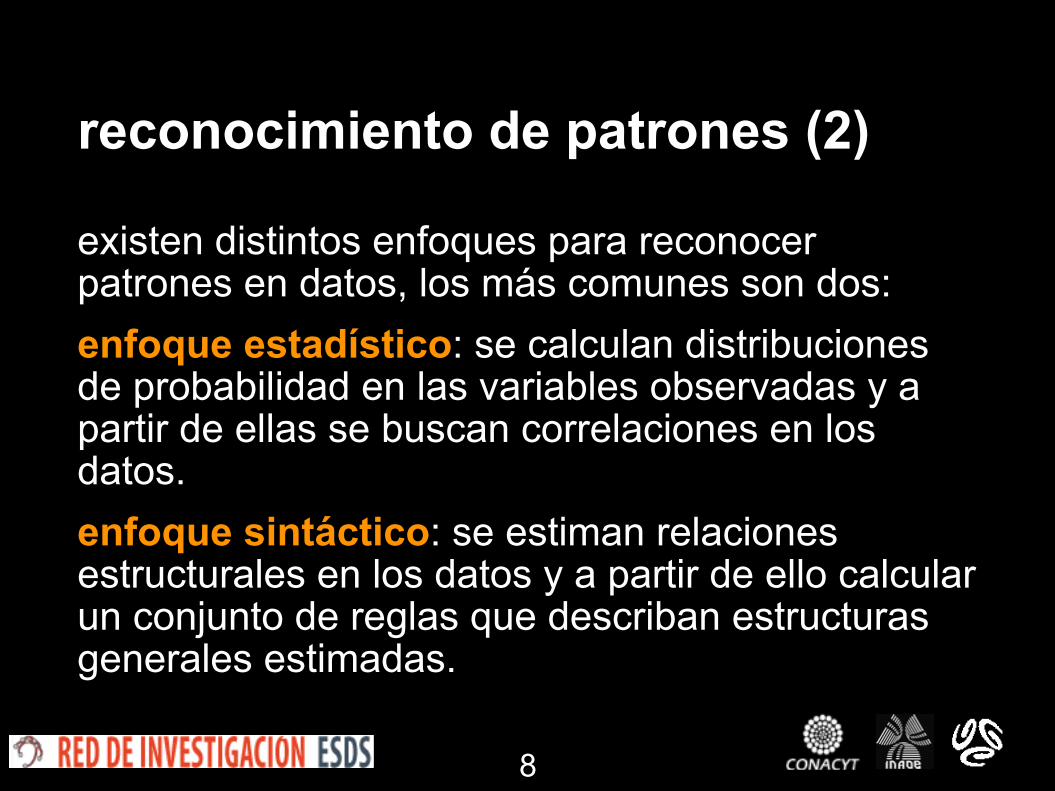
existen distintos enfoques para reconocer patrones en datos, los más comunes son dos: enfoque estadístico: se calculan distribuciones de probabilidad en las variables observadas y a partir de ellas se buscan correlaciones en los datos. enfoque sintáctico: se estiman relaciones estructurales en los datos y a partir de ello calcular un conjunto de reglas que describan estructuras generales estimadas.
8
reconocimiento de patrones (2)
9
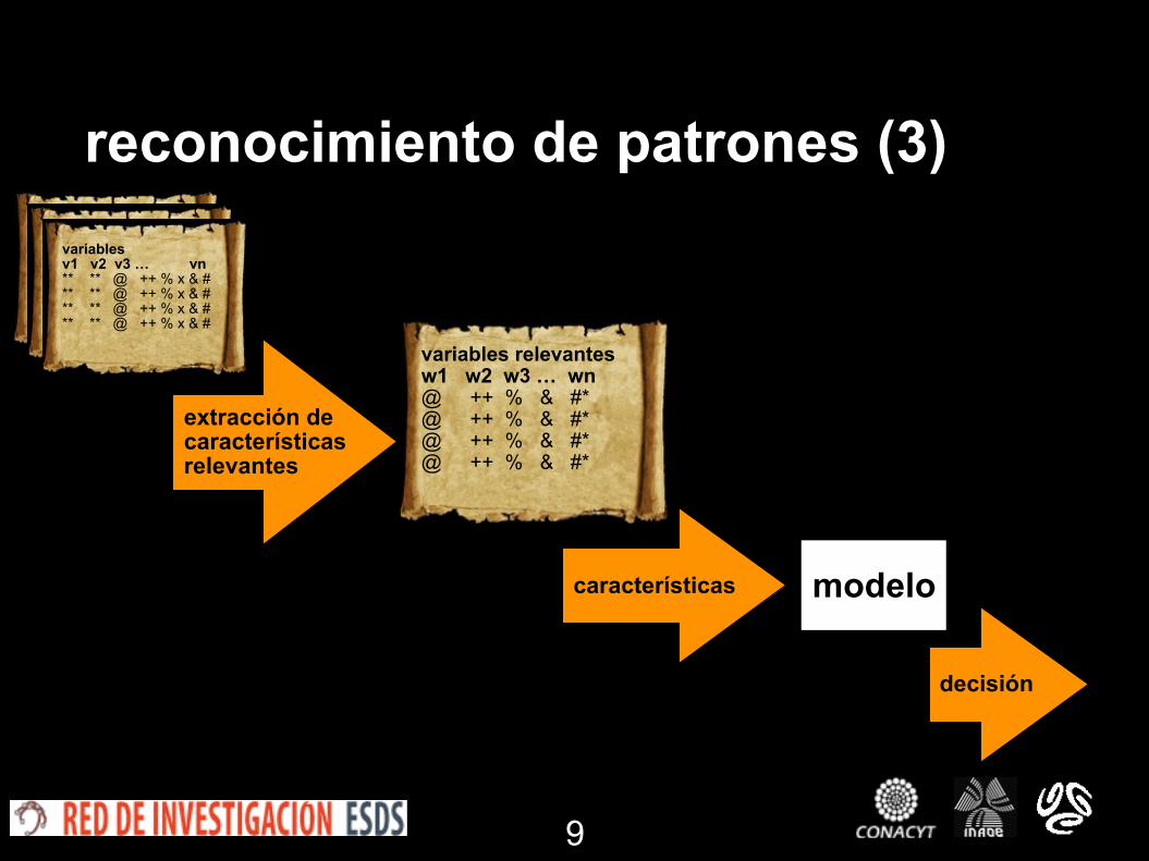
reconocimiento de patrones (3)variables v1 v2 v3 … vn ** ** @ ++ % x & # ** ** @ ++ % x & # ** ** @ ++ % x & # ** ** @ ++ % x & #
variables relevantes w1 w2 w3 … wn @ ++ % & #* @ ++ % & #* @ ++ % & #* @ ++ % & #*
extracción de características relevantes
variables v1 v2 v3 … vn ** ** @ ++ % x & # ** ** @ ++ % x & # ** ** @ ++ % x & # ** ** @ ++ % x & #
variables v1 v2 v3 … vn ** ** @ ++ % x & # ** ** @ ++ % x & # ** ** @ ++ % x & # ** ** @ ++ % x & #
características modelo
decisión
10
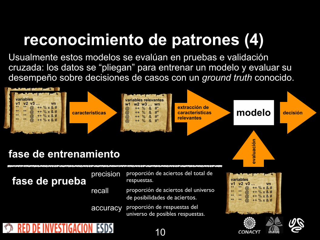
reconocimiento de patrones (4)
variables v1 v2 v3 … vn ** ** @ ++ % x & # ** ** @ ++ % x & # ** ** @ ++ % x & # ** ** @ ++ % x & #
variables relevantes w1 w2 w3 … wn @ ++ % & #* @ ++ % & #* @ ++ % & #* @ ++ % & #*
extracción de características relevantes
variables v1 v2 v3 … vn ** ** @ ++ % x & # ** ** @ ++ % x & # ** ** @ ++ % x & # ** ** @ ++ % x & #
variables v1 v2 v3 … vn ** ** @ ++ % x & # ** ** @ ++ % x & # ** ** @ ++ % x & # ** ** @ ++ % x & #
características modelo decisión
eval
uaci
ón
fase de entrenamiento
fase de prueba
Usualmente estos modelos se evalúan en pruebas e validación cruzada: los datos se “pliegan” para entrenar un modelo y evaluar su desempeño sobre decisiones de casos con un ground truth conocido.
precision proporción de aciertos del total de respuestas.
recall proporción de aciertos del universo de posibilidades de aciertos.
accuracy proporción de respuestas del universo de posibles respuestas.

ejemplos

12
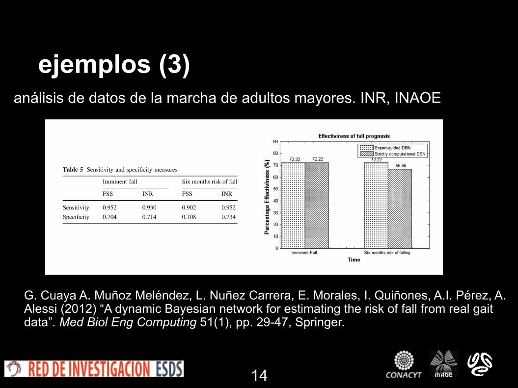
ejemplos (1)análisis de datos de la marcha de adultos mayores. INR, INAOE
Table 1: Number of calls and class associated to them based on psychiatric evaluations. There is alsoadditional data (last column) where there is no class associated.
Severe Moderate Mild Mild AdditionalPatient Depression Depression Depression Normal Manic Total DataP0201 – – 149 149 – 298 435P0302 135 – – 99 – 234 199P0702 – 112 39 – – 151 116P0902 – 142 – 161 – 303 178P1002 – – 35 – 162 197 28
All 135 254 223 409 162 1183 956
information from five patients.Table 1 shows the number of class and class associated to
them based on psychiatric evaluations. It can be seen thatwe have a di↵erent number of calls per patient and per statemoods. The table also shows additional data (last column)indicating the number of phone calls that we have that arenot associated to any state mood as they were performedoutside the 7 days window of the psychiatric assessments.
4. FEATURE SELECTIONFeature selection from smartphone sensory data is proba-
bly the most important factor to consider in order to improvethe recognition performance of machine learning tools. Inthe following subsections, we describe the most representa-tive techniques for extracting time- and frequency domainfeatures from accelerometer raw data and prosodic- and en-ergy features extracted from speech.
Table 2: Features selected for the accelerometer sen-sor signals.Time Domain Frequency Domain(1) Magnitude (1) FFT Energy,(2) Signal magnitude area (2) FFT Mean Energy,(3) Root-Mean-Square (RMS) (3) FFT StdDev Energy,(4) Variance Sum (4) Peak Power,(5) Curve Length, (5) Peak DFT Bin,(6) Non Linear Energy, (6) Peak Magnitude,(7-14) For the 3 axes: (7) Entropy,Variance, Mean, Max, Min, (8) DFTStd. Dev., Absolute, (9) Freq.Dom. Entropy,Median, a dn Range (10)Freq.Dom. Entropy(15-20) Mean and Std. Dev. with DFT,of X, Y and Z axis.For all 20 features, weotained the Min, Max, andMean For all: Min, Max, MeanTotal: 60 Total: 30
4.1 Accelerometer signal features in time-domain(TD)
In order to quantify motor activities from the smartphone,acceleration readings collected during conversation (includ-ing picking up the phone, starting and finishing the call, andreplacing the phone into the holder) were used in our anal-yses. These periods during conversation determine mean-ingful changes of acceleration values. We captured 3-axiallinear acceleration continuously at rates which varied due to
Android system operating conditions, such as system loadand battery levels. In this study, the accelerometer signalswere resampled at a fixed rate of 5 Hz. The accelerometerfeatures proposed in this paper, shown in Table 2, are quitepopular amongst practitioners in the field, and were used asthe basis for identifying periods of activity. To reduce thee↵ect of spikes and noise from accelerometer signal, statis-tical metrics such as mean and median were applied over awindow size of 128 samples.Other features included the root-mean-square (RMS) ac-
celeration for the period of conversation, as an indication ofthe time-averaged power in the signal. The RMS of a signalxi
, yi
and zi
represents a sequence of N=128 discrete valuesobtained using Equation 1 where t1 and t
n
denote the startand the end time of accelerometer readings.
accRMS =
Ptnt1
acc(t)2
t
n
� t1
! 12
(1)
The RMS results demonstrate di↵erences in the motor ac-tivity during the phone conversation. The lower the RMSvalue, the lower the motor response which is manifestedin depressed patients, whereas patients in the manic phaseshow elevated levels, as shown in Figure 1 i).Another suitable measure for phone activities, is the nor-
malized signal magnitude area (SMA) that was used as thebasis for identifying periods of activity during phone conver-satios, where x(t), y(t), and z(t) are the acceleration signalsfrom each axis with respect to time t as denoted by Equa-tion 2.
SMA =1t
Zt
o
x(t)|dt+Z
t
o
y(t)|dt+Z
t
o
x(t)|dt (2)
An example using SMA is presented in Figure 1 ii) wherechanges of motor activity can be compared in two states ofthe disease, transition from mild depressive state to normalstate. The graph inlcudes of number of phone calls in bothstates (n=140).Also, feature like Signal Vector Magnitude (SVM) have
been used to measure the degree of activity intensity andvelocity of phone movement during the phone conversationand was obtained using Equation 3.
SVM =1n
nX
i=1
qx
2i
+ y
2i
+ z
2i
(3)
Furthermore, in order to capture abrupt changes of phoneactivity during the phone conversation we used Averaged
2.2 Relevant variables
BNs and DBNs, being rooted in classical statistics, benefit
from a large number of observations and few variablesfrom those observations to identify significant probabilistic
relationships. A number of methods have been proposed to
alleviate problems with high-dimensional data when only asmall number of instances are available, such as for
instance oversampling and reduction of dimensionality.
Reduction of dimensionality can be achieved by featureselection strategies dropping a subset of variables consid-
ered to be less informative. In this work, we reduce the
dimensionality of our problem in two different ways: first,by keeping only those gait variables picked by an expert,
and second, by applying a well-known feature selection
algorithm, namely forward sequential selection (FSS), to
filter the gait variables with low predictive value from the
set of gait parameters acquired with the GaitRite system.Accordingly, we have built two DBNs for prediction of
fall from two different reduced sets of variables of human
gait. The first model is expert-guided and capitalizes on theset of variables identified by gait analysis experts from the
Human Motion Analysis Laboratory of the INR as perti-
nent for figuring out the risk of falling. These variables areshown in the top half of Table 2.
The second model is strictly computational and isfounded on the set of relevant variables as automatically
selected by the FSS algorithm [21]. The FSS algorithm was
run taking into consideration all the records from the 18patients, that is, all 66 records added up in Table 2. In this
case, the FSS algorithm achieves a reduction of the original
31 variables in Table 1 to 7 relevant variables. Thesevariables are shown in the bottom half of Table 2.
2.2.1 Forward sequential selection
Let X be a matrix whose rows correspond to points (or
observations) and columns correspond to features (or pre-dictor variables). And let Y be a column vector of response
values or class labels for each observation in X. FSS starts
with an empty feature or variable set. It then creates can-didate feature subsets by adding each of the features not yet
selected. For each candidate feature subset, FSS performs a
tenfold cross-validation, by repeatedly calling an evalua-tion function, called FUN, that defines the CRITERIONthat FSS uses to select features and determines when to
stop. See Eq. (1)
Table 1 Spatio-temporal gait parameters obtained with the GaitRitesystem
No. Parameter (unit of measure)
1 Walking distance (cm)
2 Ambulation time (s)
3 Walking velocity (cm/s)
4 Mean normalized velocity
5 Number of steps
6 Cadence
7 Left and right step time differential (s)
8 Left and right step length differential (cm)
9 Left and right cycle time differential (s)
10 Left step time (s)
11 Right step time (s)
12 Mean step time (s)
13 Mean step cycle time (s)
14 Left step length (cm)
15 Right step length (cm)
16 Left stride length (cm)
17 Right stride length (cm)
18 Base of support left step (cm)
19 Base of support right step (cm)
20 Percentage of single support left (%GC)
21 Percentage of single support right (%GC)
22 Percentage of double support left (%GC)
23 Percentage of double support right (%GC)
24 Left swing percentage (%GC)
25 Right swing percentage (%GC)
26 Left stance percentage (%GC)
27 Right stance percentage (%GC)
28 Step length/extremity length ratio left
29 Step Length/extremity length ratio right
30 Left toe in/out angle (!)
31 Right toe in/out angle (!)
Table 2 Relevant variables and their abbreviated names
CAD Cadence
Variables selected by gait analysis experts
LPI Left step length (cm)
LPD Right step length (cm)
BSI Base of support left step(cm)
LPCI Left stride length (cm)
LPCD Right stride length (cm)
BSD Base of support right step(cm)
Variables selected by FSS
TPD Right step time (s)
BSI Base of support left step(cm)
BSD Base of support right step(cm)
SDI Left double support (%GC)
RPED Right step/extremity ratio
TIOI Left toe in/out angle (!)
TIOD Right toe in/out angle (!)
Med Biol Eng Comput
123

13
ejemplos (2)análisis de datos de la marcha de adultos mayores. INR, INAOE
G. Cuaya A. Muñoz Meléndez, L. Nuñez Carrera, E. Morales, I. Quiñones, A.I. Pérez, A. Alessi (2012) “A dynamic Bayesian network for estimating the risk of fall from real gait data”. Med Biol Eng Computing 51(1), pp. 29-47, Springer.
Table 1: Number of calls and class associated to them based on psychiatric evaluations. There is alsoadditional data (last column) where there is no class associated.
Severe Moderate Mild Mild AdditionalPatient Depression Depression Depression Normal Manic Total DataP0201 – – 149 149 – 298 435P0302 135 – – 99 – 234 199P0702 – 112 39 – – 151 116P0902 – 142 – 161 – 303 178P1002 – – 35 – 162 197 28
All 135 254 223 409 162 1183 956
information from five patients.Table 1 shows the number of class and class associated to
them based on psychiatric evaluations. It can be seen thatwe have a di↵erent number of calls per patient and per statemoods. The table also shows additional data (last column)indicating the number of phone calls that we have that arenot associated to any state mood as they were performedoutside the 7 days window of the psychiatric assessments.
4. FEATURE SELECTIONFeature selection from smartphone sensory data is proba-
bly the most important factor to consider in order to improvethe recognition performance of machine learning tools. Inthe following subsections, we describe the most representa-tive techniques for extracting time- and frequency domainfeatures from accelerometer raw data and prosodic- and en-ergy features extracted from speech.
Table 2: Features selected for the accelerometer sen-sor signals.Time Domain Frequency Domain(1) Magnitude (1) FFT Energy,(2) Signal magnitude area (2) FFT Mean Energy,(3) Root-Mean-Square (RMS) (3) FFT StdDev Energy,(4) Variance Sum (4) Peak Power,(5) Curve Length, (5) Peak DFT Bin,(6) Non Linear Energy, (6) Peak Magnitude,(7-14) For the 3 axes: (7) Entropy,Variance, Mean, Max, Min, (8) DFTStd. Dev., Absolute, (9) Freq.Dom. Entropy,Median, a dn Range (10)Freq.Dom. Entropy(15-20) Mean and Std. Dev. with DFT,of X, Y and Z axis.For all 20 features, weotained the Min, Max, andMean For all: Min, Max, MeanTotal: 60 Total: 30
4.1 Accelerometer signal features in time-domain(TD)
In order to quantify motor activities from the smartphone,acceleration readings collected during conversation (includ-ing picking up the phone, starting and finishing the call, andreplacing the phone into the holder) were used in our anal-yses. These periods during conversation determine mean-ingful changes of acceleration values. We captured 3-axiallinear acceleration continuously at rates which varied due to
Android system operating conditions, such as system loadand battery levels. In this study, the accelerometer signalswere resampled at a fixed rate of 5 Hz. The accelerometerfeatures proposed in this paper, shown in Table 2, are quitepopular amongst practitioners in the field, and were used asthe basis for identifying periods of activity. To reduce thee↵ect of spikes and noise from accelerometer signal, statis-tical metrics such as mean and median were applied over awindow size of 128 samples.Other features included the root-mean-square (RMS) ac-
celeration for the period of conversation, as an indication ofthe time-averaged power in the signal. The RMS of a signalxi
, yi
and zi
represents a sequence of N=128 discrete valuesobtained using Equation 1 where t1 and t
n
denote the startand the end time of accelerometer readings.
accRMS =
Ptnt1
acc(t)2
t
n
� t1
! 12
(1)
The RMS results demonstrate di↵erences in the motor ac-tivity during the phone conversation. The lower the RMSvalue, the lower the motor response which is manifestedin depressed patients, whereas patients in the manic phaseshow elevated levels, as shown in Figure 1 i).Another suitable measure for phone activities, is the nor-
malized signal magnitude area (SMA) that was used as thebasis for identifying periods of activity during phone conver-satios, where x(t), y(t), and z(t) are the acceleration signalsfrom each axis with respect to time t as denoted by Equa-tion 2.
SMA =1t
Zt
o
x(t)|dt+Z
t
o
y(t)|dt+Z
t
o
x(t)|dt (2)
An example using SMA is presented in Figure 1 ii) wherechanges of motor activity can be compared in two states ofthe disease, transition from mild depressive state to normalstate. The graph inlcudes of number of phone calls in bothstates (n=140).Also, feature like Signal Vector Magnitude (SVM) have
been used to measure the degree of activity intensity andvelocity of phone movement during the phone conversationand was obtained using Equation 3.
SVM =1n
nX
i=1
qx
2i
+ y
2i
+ z
2i
(3)
Furthermore, in order to capture abrupt changes of phoneactivity during the phone conversation we used Averaged
precision of 70 % in predicting both imminent falls and 6months risk of falling.
Both models were evaluated using leave-one-out cross
validation (LOOCV). The LOOCV is a technique thatfacilitates estimation of performance of a predictive model
when the available number of samples is low, as it occurs
in this case where data from 18 patients only are available.During LOOCV, observations are left out one at a time and
a model instance is trained with the remaining observations
and tested on the observation left out. This procedure isrepeated for all of the observations and the predictive
power of the model is considered to be the average of all
the model instances.Thereby, for each of the two conceptual models (the
expert selection based and the FSS selection based), 18
different model instances were built using data from 17patients and tested on the remaining patient on the most
probable value of the node fall, 0 = no fall or 1 = fall. Notethat here we exclude all observations corresponding to the
longitudinal assessments for a given subject at a time,
rather than dropping every single observation separately.Figure 4 shows the DBNs built by Hugin using human gait
data.
The effectiveness of the forecasting of imminent fallsand 6 months risk of falling is defined as the ratio of the
number of falls predicted by the model divided by the
number of falls that actually occurred in the correspondingtime interval.
The effectiveness of the forecasting of imminent falls
and 6 months risk of falling were 72.22 % in both cases forthe DBN model built upon the variables selected by the
domain experts, and 72.22 and 66.66 % for the DBN built
upon the variables that were automatically selected withFSS algorithm. These results are summarized in Fig. 5.
The effectiveness of both models is presented without
confidence intervals due to the small number of samples.Tables 3 and 4 detail he confusion matrices for the two
conceptual models at the two time intervals considered;
imminent and 6 months, respectively. The confusionmatrices presented have been built from the agglomerate
results during the LOOCV.
Finally, the sensitivity and specificity of the conceptualmodels have been estimated. Sensitivity (also called recall
rate in some fields) measures the proportion of actual
positives which are correctly identified over the total realpositives (i.e. the percentage of elders who are correctly
(a) DBN based on expert’s variables.
(b) DBN based on automatic selectedvariables.
Fig. 4 a DBN based on gait parameters selected by experts, b DBNbased on gait parameters selected by the FSS algorithm. See Table 2for the definition of abbreviations
Fig. 5 Comparison of the prognosis results of the two models
Med Biol Eng Comput
123
14
ejemplos (3)análisis de datos de la marcha de adultos mayores. INR, INAOE
Table 1: Number of calls and class associated to them based on psychiatric evaluations. There is alsoadditional data (last column) where there is no class associated.
Severe Moderate Mild Mild AdditionalPatient Depression Depression Depression Normal Manic Total DataP0201 – – 149 149 – 298 435P0302 135 – – 99 – 234 199P0702 – 112 39 – – 151 116P0902 – 142 – 161 – 303 178P1002 – – 35 – 162 197 28
All 135 254 223 409 162 1183 956
information from five patients.Table 1 shows the number of class and class associated to
them based on psychiatric evaluations. It can be seen thatwe have a di↵erent number of calls per patient and per statemoods. The table also shows additional data (last column)indicating the number of phone calls that we have that arenot associated to any state mood as they were performedoutside the 7 days window of the psychiatric assessments.
4. FEATURE SELECTIONFeature selection from smartphone sensory data is proba-
bly the most important factor to consider in order to improvethe recognition performance of machine learning tools. Inthe following subsections, we describe the most representa-tive techniques for extracting time- and frequency domainfeatures from accelerometer raw data and prosodic- and en-ergy features extracted from speech.
Table 2: Features selected for the accelerometer sen-sor signals.Time Domain Frequency Domain(1) Magnitude (1) FFT Energy,(2) Signal magnitude area (2) FFT Mean Energy,(3) Root-Mean-Square (RMS) (3) FFT StdDev Energy,(4) Variance Sum (4) Peak Power,(5) Curve Length, (5) Peak DFT Bin,(6) Non Linear Energy, (6) Peak Magnitude,(7-14) For the 3 axes: (7) Entropy,Variance, Mean, Max, Min, (8) DFTStd. Dev., Absolute, (9) Freq.Dom. Entropy,Median, a dn Range (10)Freq.Dom. Entropy(15-20) Mean and Std. Dev. with DFT,of X, Y and Z axis.For all 20 features, weotained the Min, Max, andMean For all: Min, Max, MeanTotal: 60 Total: 30
4.1 Accelerometer signal features in time-domain(TD)
In order to quantify motor activities from the smartphone,acceleration readings collected during conversation (includ-ing picking up the phone, starting and finishing the call, andreplacing the phone into the holder) were used in our anal-yses. These periods during conversation determine mean-ingful changes of acceleration values. We captured 3-axiallinear acceleration continuously at rates which varied due to
Android system operating conditions, such as system loadand battery levels. In this study, the accelerometer signalswere resampled at a fixed rate of 5 Hz. The accelerometerfeatures proposed in this paper, shown in Table 2, are quitepopular amongst practitioners in the field, and were used asthe basis for identifying periods of activity. To reduce thee↵ect of spikes and noise from accelerometer signal, statis-tical metrics such as mean and median were applied over awindow size of 128 samples.Other features included the root-mean-square (RMS) ac-
celeration for the period of conversation, as an indication ofthe time-averaged power in the signal. The RMS of a signalxi
, yi
and zi
represents a sequence of N=128 discrete valuesobtained using Equation 1 where t1 and t
n
denote the startand the end time of accelerometer readings.
accRMS =
Ptnt1
acc(t)2
t
n
� t1
! 12
(1)
The RMS results demonstrate di↵erences in the motor ac-tivity during the phone conversation. The lower the RMSvalue, the lower the motor response which is manifestedin depressed patients, whereas patients in the manic phaseshow elevated levels, as shown in Figure 1 i).Another suitable measure for phone activities, is the nor-
malized signal magnitude area (SMA) that was used as thebasis for identifying periods of activity during phone conver-satios, where x(t), y(t), and z(t) are the acceleration signalsfrom each axis with respect to time t as denoted by Equa-tion 2.
SMA =1t
Zt
o
x(t)|dt+Z
t
o
y(t)|dt+Z
t
o
x(t)|dt (2)
An example using SMA is presented in Figure 1 ii) wherechanges of motor activity can be compared in two states ofthe disease, transition from mild depressive state to normalstate. The graph inlcudes of number of phone calls in bothstates (n=140).Also, feature like Signal Vector Magnitude (SVM) have
been used to measure the degree of activity intensity andvelocity of phone movement during the phone conversationand was obtained using Equation 3.
SVM =1n
nX
i=1
qx
2i
+ y
2i
+ z
2i
(3)
Furthermore, in order to capture abrupt changes of phoneactivity during the phone conversation we used Averaged
G. Cuaya A. Muñoz Meléndez, L. Nuñez Carrera, E. Morales, I. Quiñones, A.I. Pérez, A. Alessi (2012) “A dynamic Bayesian network for estimating the risk of fall from real gait data”. Med Biol Eng Computing 51(1), pp. 29-47, Springer.
precision of 70 % in predicting both imminent falls and 6months risk of falling.
Both models were evaluated using leave-one-out cross
validation (LOOCV). The LOOCV is a technique thatfacilitates estimation of performance of a predictive model
when the available number of samples is low, as it occurs
in this case where data from 18 patients only are available.During LOOCV, observations are left out one at a time and
a model instance is trained with the remaining observations
and tested on the observation left out. This procedure isrepeated for all of the observations and the predictive
power of the model is considered to be the average of all
the model instances.Thereby, for each of the two conceptual models (the
expert selection based and the FSS selection based), 18
different model instances were built using data from 17patients and tested on the remaining patient on the most
probable value of the node fall, 0 = no fall or 1 = fall. Notethat here we exclude all observations corresponding to the
longitudinal assessments for a given subject at a time,
rather than dropping every single observation separately.Figure 4 shows the DBNs built by Hugin using human gait
data.
The effectiveness of the forecasting of imminent fallsand 6 months risk of falling is defined as the ratio of the
number of falls predicted by the model divided by the
number of falls that actually occurred in the correspondingtime interval.
The effectiveness of the forecasting of imminent falls
and 6 months risk of falling were 72.22 % in both cases forthe DBN model built upon the variables selected by the
domain experts, and 72.22 and 66.66 % for the DBN built
upon the variables that were automatically selected withFSS algorithm. These results are summarized in Fig. 5.
The effectiveness of both models is presented without
confidence intervals due to the small number of samples.Tables 3 and 4 detail he confusion matrices for the two
conceptual models at the two time intervals considered;
imminent and 6 months, respectively. The confusionmatrices presented have been built from the agglomerate
results during the LOOCV.
Finally, the sensitivity and specificity of the conceptualmodels have been estimated. Sensitivity (also called recall
rate in some fields) measures the proportion of actual
positives which are correctly identified over the total realpositives (i.e. the percentage of elders who are correctly
(a) DBN based on expert’s variables.
(b) DBN based on automatic selectedvariables.
Fig. 4 a DBN based on gait parameters selected by experts, b DBNbased on gait parameters selected by the FSS algorithm. See Table 2for the definition of abbreviations
Fig. 5 Comparison of the prognosis results of the two models
Med Biol Eng Comput
123
identified as fallers). Specificity measures the proportion of
negatives which are correctly identified over the total realnegatives (i.e. the percentage of elders who are correctly
identified as not fallers). The sensitivity and specificity of
both conceptual models are presented in Table 5.
4 Discussion
This research aims at generating a model for prediction of
fall in the elderly that capitalizes on quantifying probabi-listic dependencies among gait variables. Our objective has
been to develop an intelligible model for non-experts in
probabilistic reasoning that afford them with complemen-tary information. Distinctly from related work [17, 38], our
model incorporates people’s gait degradation as captured
by assessment instruments and learns the probabilistic
relationships among the variables recorded by such
instruments to forecast the risk of fall of an elder.A strictly computational model based on selected
information extracted from gait assessments was compared
with an analogous model based on information drawn fromthe gait assessments by experts. For estimating the risk of
fall, the computational feature selection method picked out
variables of human gait that were not considered relevantby the experts. Nevertheless, both conceptual models
yielded comparable performances.Although the model based upon automatic feature
selection exhibits lower performance for the 6 monthsprediction, this model emerges from a very limited datasetand still afforded competitive performance. In this sense,
the experts base his/her selection on an experience cer-
tainly spanning more observations than those in the dataset.In general, the larger the training dataset the more reliable
model can be expected.
This work demonstrates the feasibility of employingprobabilistic models such as DBNs to estimate the proba-
bility of a fall. We have presented two probabilistic models
of fall risk assessment that were developed from actualrecords of spatio-temporal gait parameters. To our
knowledge, these are the first probabilistic models of fall
risk assessment that exploit relationships among relevantvariables. Since a gait model is now available, it can be
applied by human gait experts and clinicians to obtain
additional elements to enrich their decisions about treat-ment and therapies to be prescribed to elders with different
degrees of gait impairment.
Note that both, the strictly computational model and theexpert-guided model achieve comparable performances as
measured by sensitivity and specificity outcomes. This can
be indicative that there is a further reduced set of variablesof human gait relevant for predicting falls, perhaps in the
intersection of the subsets of variables considered by both
models.We are currently bettering the models by enlarging the
dataset. Models for predicting falls within 12 and
18 months will be developed as we grow our cohort sizeand expand follow-up times. We will also incorporate
information from people with normal gait to compare their
assessments with those from individuals with pathologicalgait.
Acknowledgments This research was supported by the NationalInstitute for Astrophysics, Optics and Electronics (INAOE), and theMexican National Council for Science and Technology (CONACyT),through the scholarship for doctoral studies 174498. The researchersof the Human Motion Analysis Laboratory of the National Institute ofRehabilitation in Mexico provided the gait data to develop the modelspresented in this work, under the research grant 01-042 of CONA-CyT-Health Sector Fund 2003.
Table 3 Confusion matrix to prognostic of imminent falls
Negative Positive
Predicted using information get with computational techniques
Actual
Negative 31 2
Positive 13 9
Predicted with information get of experts
Actual
Negative 30 3
Positive 12 10
Table 4 Confusion matrix to prognostic of 6 months risk of fall
Negative Positive
Predicted using information get withcomputational techniques
Actual
Negative 34 4
Positive 14 3
Predicted with information get of experts
Actual
Negative 36 2
Positive 13 4
Table 5 Sensitivity and specificity measures
Imminent fall Six months risk of fall
FSS INR FSS INR
Sensitivity 0.952 0.930 0.902 0.952
Specificity 0.704 0.714 0.708 0.734
Med Biol Eng Comput
123

Muchas gracias!
Más información
Angélica Muñoz MeléndezCoordinación de Ciencias Computacionales
Instituto Nacional de Astrofísica, Óptica y Electrónica, INAOE
ccc.inaoep.mx/~munoz
15
Top Related