


Languages
Pages
Legal


Intro to Signal Processing
• Signal– A function that conveys information
– Often thought of as a function of time
– We will consider it to be a function of “space”(spatial domain)

Intro to Signal Processing
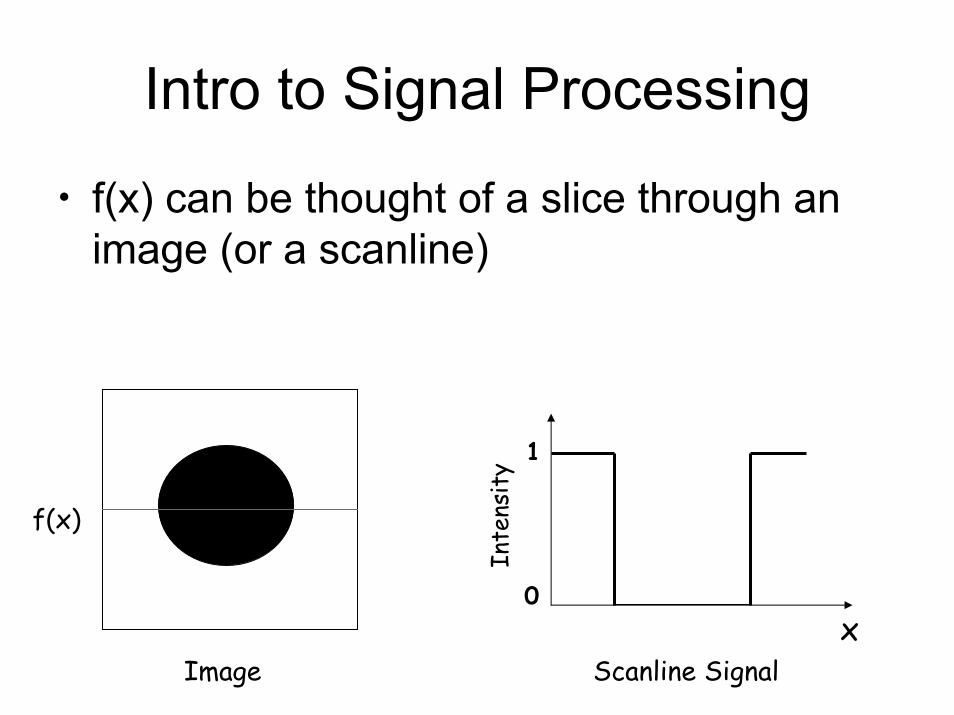
• f(x) can be thought of a slice through an image (or a scanline)
• We will consider the 1D case
• Although the concepts apply to 2D
Intro to Signal Processing
• f(x) can be thought of a slice through an image (or a scanline)
1
Inte
nsit
yf(x)
0x
Image Scanline Signal

Intro to Signal Processing
• f(x) can be thought of a slice through an image (or a scanline)
Inte
nsit
y
f(x)
ImageScanline Signal

Question
• How do we sample this signal?• In order to reconstruct it?

Sampling too little
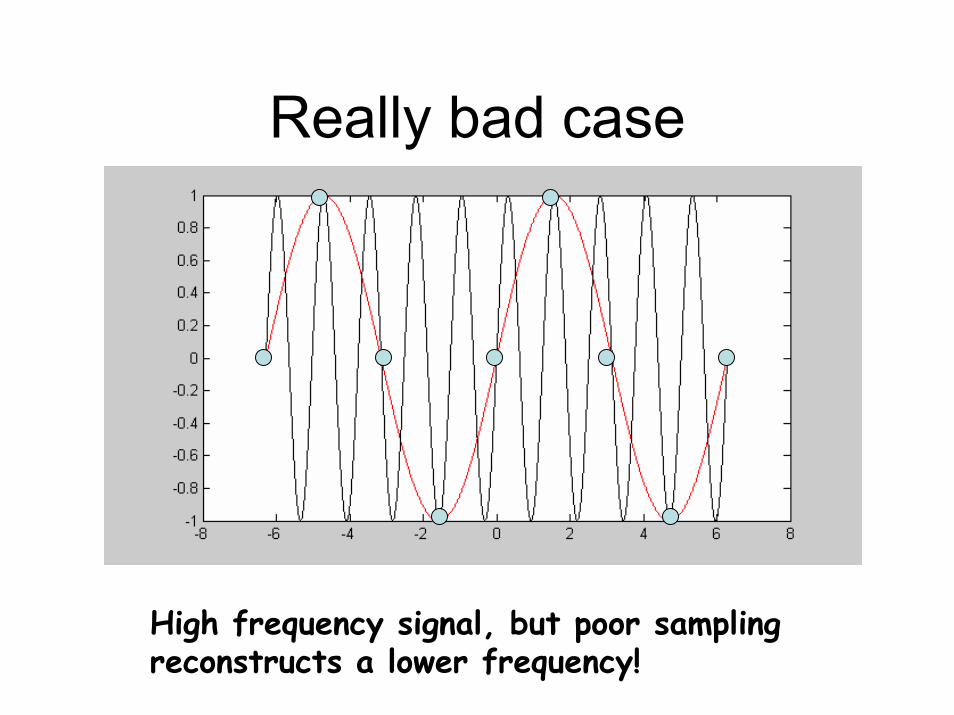
Really bad case
High frequency signal, but poor samplingreconstructs a lower frequency!

Aliasing
• Definition of word “Alias”– An assumed name– A false signal
• Reconstructing the wrong signal due to poor sampling is called “Aliasing”
• Trying to avoid aliasing is “Anti-aliasing”

Just take more samples you say!

Consider this signal
You need an infinite number
of samples!
f(x)
xHow many samples do you need?

Sampling Theory
• Provides a framework to describe how a function needs to be sampled in order to reconstruct it
• It will require us to consider the function’s frequency decomposition

Frequency Domain
• A spatial signal f(x) can be represented as a sum of phase-shifted sine waves (of various amplitudes)
• May contain any frequency (infinitely many)
• Each f(x) has one representation in the frequency domain (and vice versa)

Fourier Analysis
• To compute these sine waves
• Fourier Transform of a function f(x), is F(u) – ‘u’ represents frequency– F(u) is the representation of f(x) in the
frequency domain
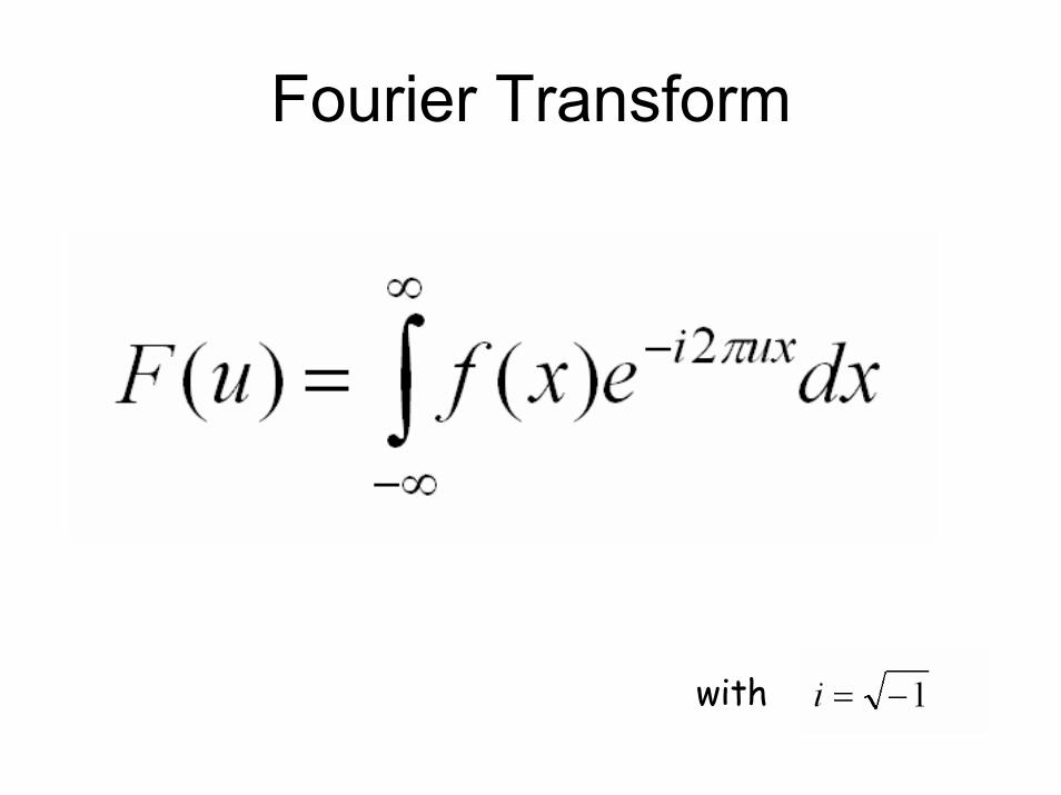
Fourier Transform
with

Fourier Transform
(Eulers formula)
we can rewrite F(u) as:
F(u) is in terms of sines (and cosines)(recall that sin(x) = cos(x-[pi/2]) )

Fourier Transform• F(u) can be written as real and imaginary components
– F(u) = R(u) + iI(u)
• Magnitude/Amplitude of the sine wave of frequency u
|F(u)| = sqrt( R(u)^2 + I(u)^2 )
• Phase-shift (sometimes called phase angle), φ, of frequency (u)
φ(u) = tan-1| I(u) / R(u) |
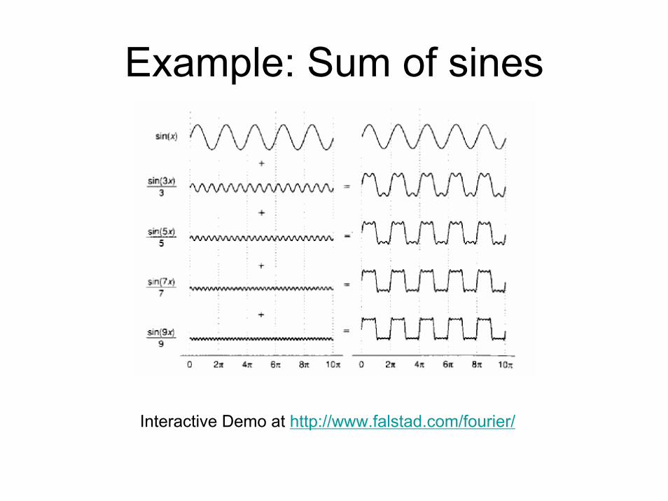
Example: Sum of sines
http://www.falstad.com/fourier/Interactive Demo at

Signal f(x)
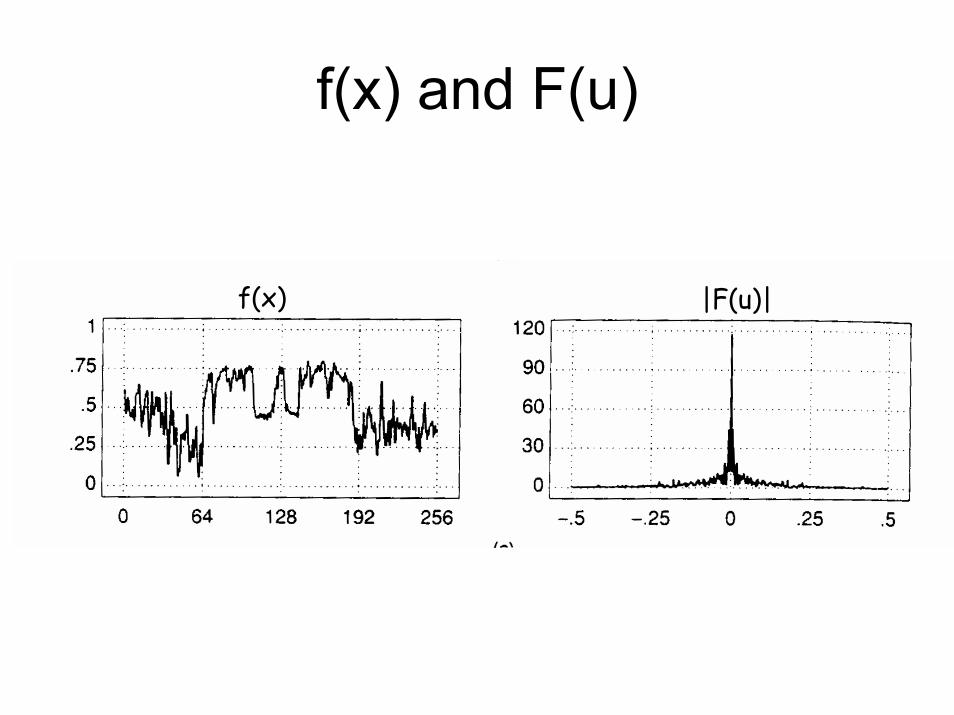
f(x) and F(u)
f(x) |F(u)|

Inverse Fourier Transform

Example

Example
Original Sum of the frequencies(using only 10 frequencies)
Example f(x) to F(u)
• Online demo http://www.jhu.edu/~signals/fourier2/index.html

f(x) -> F(u)

f(x,y) -> F(u,v)

Fourier Pairs and Properties
• We will need to know some common f(x) and their F(u)
• f(x) and F(u) are Fourier pairs
– where F(u) = F {f(x)}– there are some very interesting relationships
between f(x) and its F(u)

Some useful functions f(x)f
x
1
f(x) = 1 x>00 x<0• Step function
• Sign function
• Rectangular function
• delta function(a pulse)
0
f
f(x) = 1 x>0-1 x<0 x
1
-1
f
x
1
f(x) = 1 |x|>a0 |x|<a a-a
0δ(x) =
integral at x is 10 elsewhere
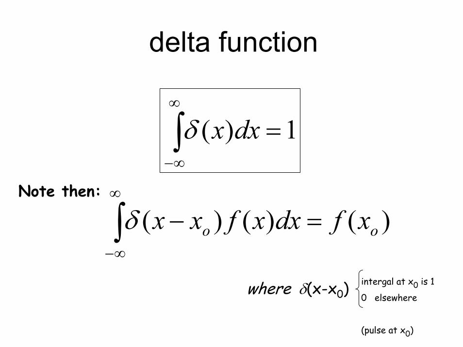
delta function
∫∞
∞−
=1)( dxxδ
Note then:
)()()(∫∞
∞−
=− oo xfdxxfxxδ
where δ(x-x0)intergal at x0 is 1
0 elsewhere
(pulse at x0)
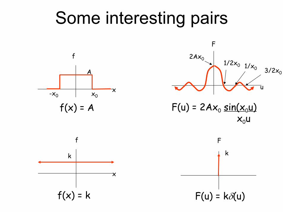
Some interesting pairs
3/2x0
x
f
A
x0-x0
f(x) = A F(u) = 2Ax0 sin(x0u)x0u
2Ax01/2x0 1/x0
u
F
x
k
f(x) = k
f
k
F(u) = kδ(u)
F

Some interesting pairsf F
x
f(x) = Acos(u0x)
A/2AA/2
-u0 u0
F(u) = Aδ(u -u0) + Aδ(u + u0)2 2
1f
-x0 x0-2x0-3x0 2x0 3x0
F1/x0
1/x0-2/x0 2/x00 - 1/x0
∑∞
−∞=
−∂=n
nxxf )()( ∑∞
−∞=
−∂=n x
nux
uF )(1)(00

Some interesting pairs
f
x2x0-2x0
A2
4A2x02
1/2x0 1/x0
u
F
F(u) = 4Ax02 sin2 (x0u)
(x0u) 2f(x) = -A2x + A2
2x0
x
f1
22/2)( σxexf −=
x
F
2/22
2)( ueuF σπσ −=
πσ 2
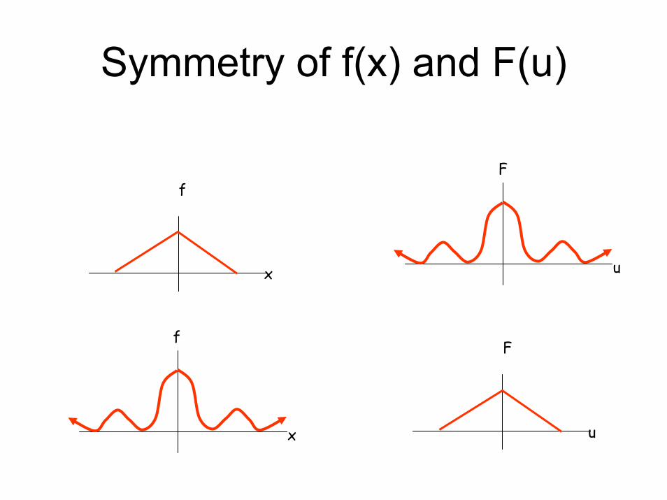
Symmetry of f(x) and F(u)
u
Ff
x
x
fF
u

Some Fourier Pairs Properties• Linearity
–F {f(x) + g(x) } = F(u) + G(u)
• Scaling
–F {f(ax) } = 1/|a| F(u/a)• Convolution
–F {f(x)*g(x) } = F(u)G(u)

Convolution of f(x) and g(x)
∫∞
∞−
∂−== ααα )()()(*)()( xgfxgxfxh
• h(x) =– for each x– flip g about x (mirror image of g . . .g(x-a) [a=-inf to inf])– h(x) = the integral of the point wise product of
f(a) and g(x-a) [a=-inf to inf]

Graphical Representation
h(x)
a = τ
h(x) = f(a)g(x-a)da h(x) = f(a)g(x-a)da

In Frequency Domain
• Convolution in spatial domain• Is a multiplication in the frequency domain
–F { f(x)*g(x) } = F(u) G(u)

Want to compute h(x) = f(x)*g(x)?
• Compute
– F(u) =F {f(x)} and G(u) =F {g(x)}– H(u) = F(u)G(u)
• Compute
– h(x) = F -1 {H(u)}

What is sampling?• Function f(x)
• Function s(x)
• Sampling can be thought of as a multiplication in the spatial domain
–Of a function f(x) with a function ofequally spaced “delta functions”, s(x)
–[s(x) is a train of delta functions]

What is sampling?• Function f(x)
• Function s(x)
• Sampling can be thought of as a multiplication in the spatial domain
–Of a function f(x) with a function ofequally spaced “delta functions”, s(x)
–[s(x) is a train of delta functions]

Sampling in Frequency Domain
• Convolution of F(u)*S(u)
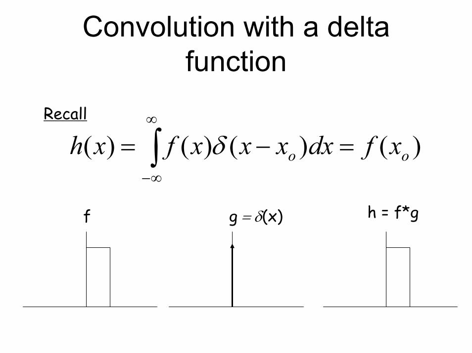
Convolution with a delta function
)()()()( oo xfdxxxxfxh =−= ∫∞
∞−
δRecall
f g h = f*g= δ(x)

Convolution with several delta functions
f*gf(x) g(x)
-T
AA
a a T-T T
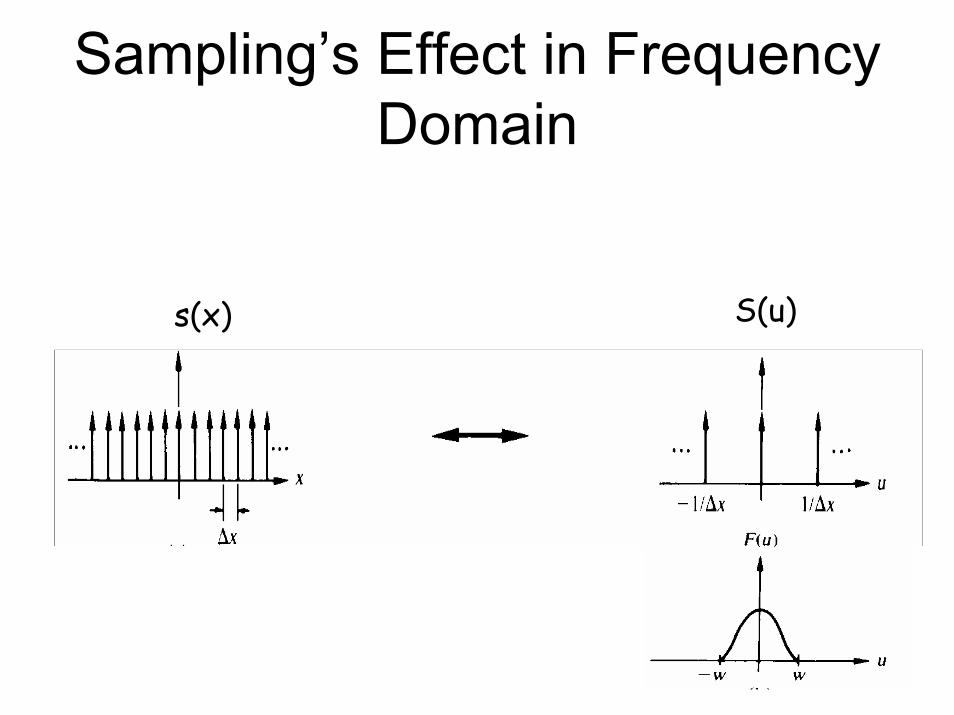
Sampling’s Effect in Frequency Domain
S(u)s(x)

F {f(x)}
Say that, f(x) has a Fourier transform, where the highestfrequency is W
(functions with a finite # of frequencies arecalled “band-limited” function)

Spatial Sampling in Frequency Domain
It will duplicate F(u)at intervals 1/∆x

What does this mean?
We need to chose ∆xsuch that ∆x <= 1/2W
That is to say, we need to sample at least twice the highest frequency!

Sampling at 2W or higher
1/2W’ 2W’2W’W’ is slightly larger than W
Twice the highest frequency isoften called the “Nyquist Rate”
Nyquist Rate
This is a very important discovery.
It tells us how we mustsample a function in order
to reconstruct it!

(Side Note)
• Seen these sampling rates?– 8 kHz -- phone– 16 kHz -- near high-fidelity– 44.1 kHz -- high-fidelity
• Do you know why?• Nyquist Rates

Reconstructing the Signal
F -1

Do you see why this is cool?
We have reconstructed f(x) using s(x)f(x)!We never “knew” f(x) directly!

Well, almost• We did get help from G(u)
– The “Box Filter”•
And the Fourier Transform
– h(x) = f(x)s(x)
–F { h(x)} = H(U)
– f(x) = F -1{G(u)*H(u)}

What if we do everything in the spatial domain
• We know– F(u) = H(u)G(u)– f(x) = h(x)*g(u) H(u)G(u)
So, reconstruction in spatial domain is:
• f(x) = f(x)s(x) * F- -1{G(u)}
• What is F- -1{G(u)}?
x
f/F
u
F/fRecall this Fourier pair:

Spatial Domain Reconstruction
Convolve sampleswith an infinite sinc!!!

Remember our question?
Source2 x 2 pixels
How should we sample?
AND, that only works for“band-limited” f(x)
AnswerFor each destination pixel,take infinitely many samplesfrom the source and convolved them with a “sinc” function

BACK TO REALITY
• Nyquist rate and all that Fourier stuff is nice on paper, but here are the hard facts– Few functions are band limited– We rarely perform a real Fourier transform– And nobody is going to take infinite samples!

Back to Reality
• Image Sampling and Filtering
– Lets look at what poor sampling means
– Lets look at what different filters mean

Sampling

Poor Sampling

Filtering• Assume good sampling
• How do we “combine” our samples to create a new pixel?
• This is equivalent to “filtering” in the frequency domain
• For instant– Infinite samples * sinc is the best filter
• What about practical approaches
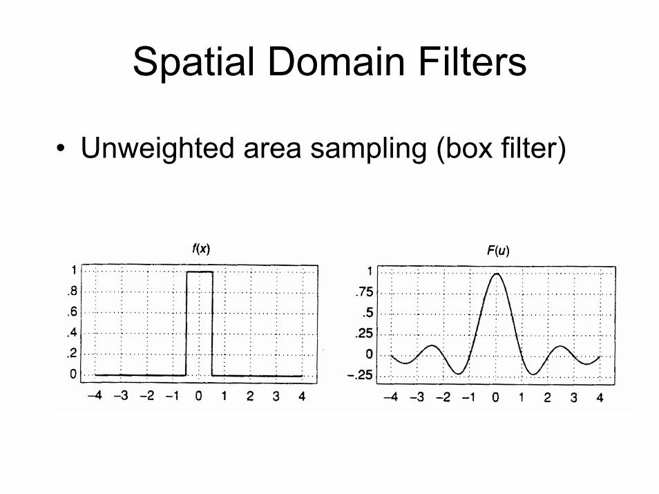
Spatial Domain Filters
• Unweighted area sampling (box filter)

Box Filter
Very bad choice!
Allows lots of unwanted“noise” . . aliasing
But its fast to do in thespatial domain.

Spatial Domain Filters
• Weighted area sampling (triangle filter)• Linear Interpolation
sinc2
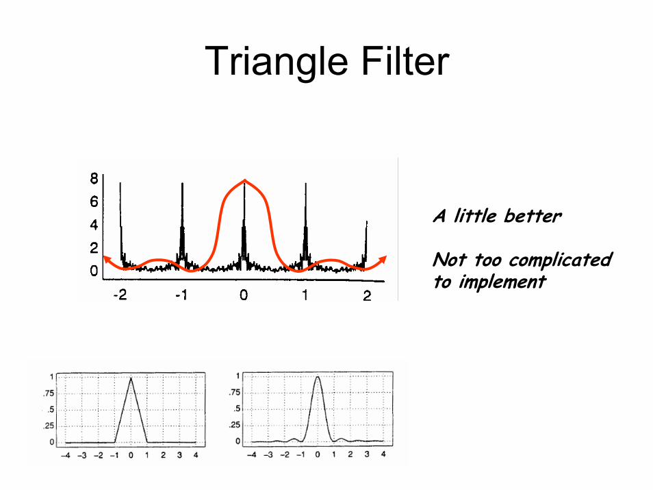
Triangle Filter
A little better
Not too complicatedto implement

Triangle Filter
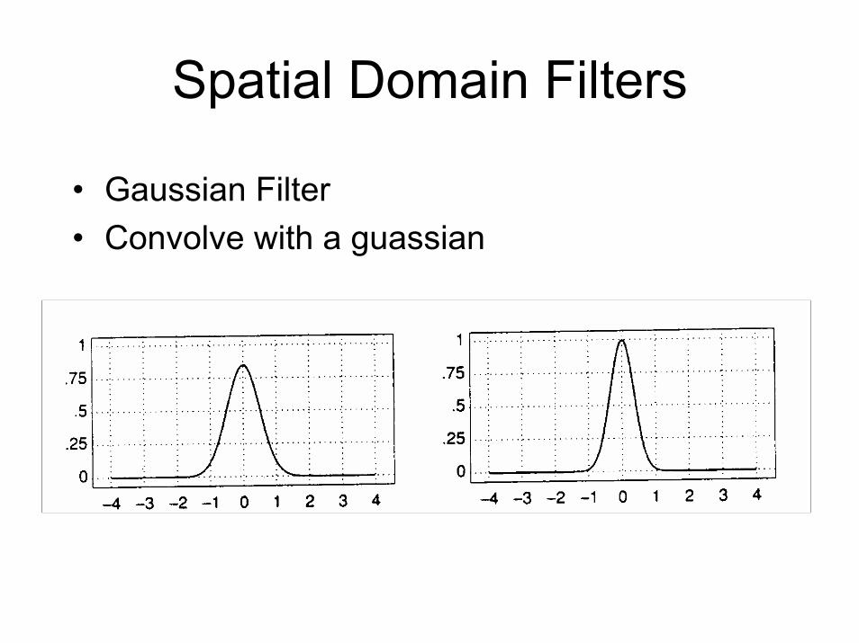
Spatial Domain Filters
• Gaussian Filter• Convolve with a guassian

Gaussian Filter
Even Better
Falls off to zerovery quickly
More complicated to implement in spatialdomain

Blurring
These filters have a “blurring” effect on signals with high frequencies

Pre-filtering
• The problem is with high frequencies
• If we don’t sample at 2 twice the highest frequency we have trouble
• We know some signals have infinite frequencies!
• Why not get rid of these frequencies, then sample?
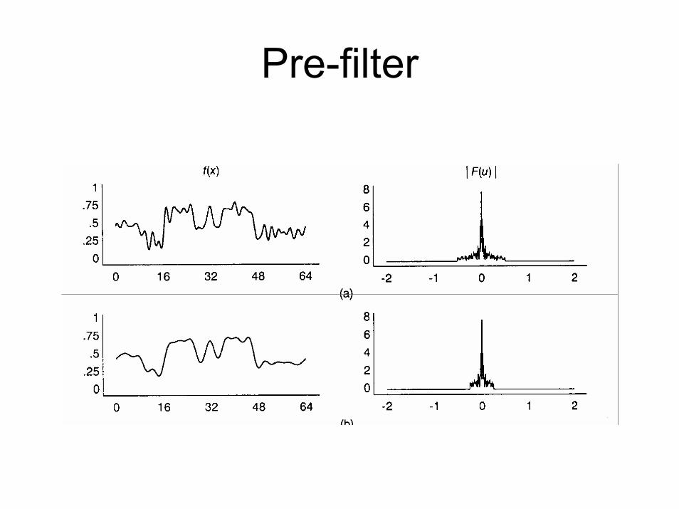
Pre-filter
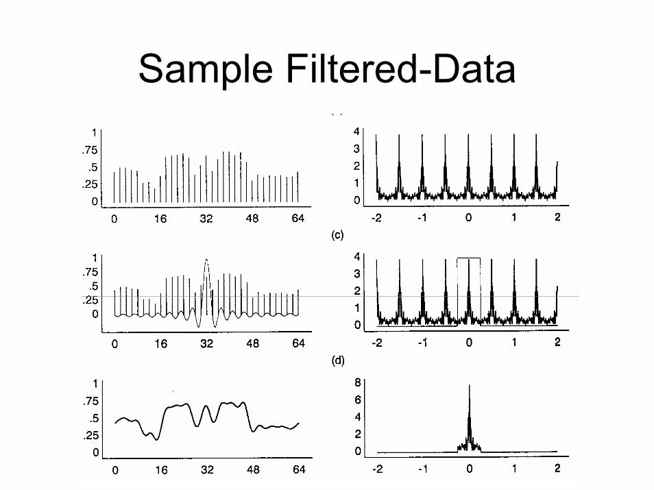
Sample Filtered-Data

Pre-filtering
• Low Pass Filter, then Sampling
• “Blurs” the image
• Allows you to faithfully reconstruct a different signal (low pass signal)
• Pretty common in Audio
Back to where we started
• We have an image
• We have transformed it
• We are sampling it– Nearest Neighbor, Bi-linear, Bi-Cubic

Post-filter or Pre-filter?
• Depends on point of view– We generally do not sample an image, then
apply a filter• We apply a filter when we sample• Pre-Filtering
– But, the source image itself is sort of a set of “samples”
• OK, we are Post-Filtering
• We are filtering

Common Sampling ApproachesNearest Neighbor
Bi-linear Interpolation
Bi-Cubic

Nearest Neighbor
• Similar to a box filter – Maybe a little worse– Allows high-frequencies– Causes excessive blurring
• Benefits– Fast
• Cheap texture-mapping hardware– Doesn’t introduce new intensity values!
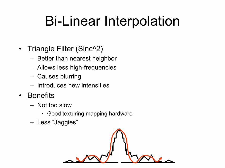
Bi-Linear Interpolation
• Triangle Filter (Sinc^2) – Better than nearest neighbor– Allows less high-frequencies– Causes blurring– Introduces new intensities
• Benefits– Not too slow
• Good texturing mapping hardware– Less “Jaggies”

Bi-Cubic Interpolation
• Similar to Gauss Filter– Better than bi-linear– Allows even less high-frequencies– Causes more blurring– Introduces new intensities
• Benefits– Slow
• Really good texturing mapping hardware– Even less “Jaggies”

Best would be a infinite sinc
• But that is too hard, infinite samples• Why not use a truncated sinc?
ringing

Don’t worry too much
• Live a good life
• Be kind to others – (especially little creatures)
• Avoid nearest neighbor
• Use bi-linear or bi-cubic sampling– Know these aren’t perfect– Use the fourier transform and prove to people that these
aren’t perfect– And be happy
Top Related