Download - Interval Estimation for Binomial Proportion, …532980/FULLTEXT01.pdfInterval Estimation for Binomial Proportion, Poisson Mean, and Negative –binomial Mean Luchen Liu Supervisor:

Interval Estimation for Binomial Proportion, Poisson Mean, and Negative

–binomial Mean

Luchen Liu

Supervisor: Rolf Larsson

Master Thesis in Statistics, May 2012

Uppsala University, Sweden

Contents

Abstract .......................................................................................................... 1 1. Introduction .............................................................................................. 2 2. Methodology .............................................................................................. 3

2.1 The Actual Coverage Probability .......................................................... 3 2.2 The Expected Length ............................................................................ 3

3. Confidence Intervals for the Binomial Proportion .................................. 4 3.1 The Standard Wald Interval................................................................... 4 3.2 Frequentist Alternative Confidence Intervals......................................... 5 3.3 The Bayesian Alternative Confidence Interval ...................................... 8 3.4 The Expected Length .......................................................................... 10 3.5 Discussion ........................................................................................... 11

4. The Confidence Interval for the Poisson Mean ..................................... 16 4.1 The Wald Interval ............................................................................... 16 4.2 Alternative Confidence Intervals ......................................................... 18 4.3 The Expected Length of The Poisson Intervals .................................... 21

5. The Confidence Interval for the Negative binomial Mean .................... 23 5.1 The Wald Interval ............................................................................... 23 5.2 Alternative Confidence Intervals ......................................................... 25 5.3 The Expected Length of The Negative-binomial Intervals ................... 28

6. Conclusions and Discussions .................................................................. 31 6.1 Conclusions ........................................................................................ 31 6.2 Discussion ........................................................................................... 31

7. Empirical examples ................................................................................. 33 7.1 Female births proportion ..................................................................... 33 7.2 The horse kick data ............................................................................. 34

1

Interval Estimation for Binomial Proportion, Poisson Mean, and Negative

–binomial Mean

Author: Luchen Liu

Supervisor: Rolf Larsson

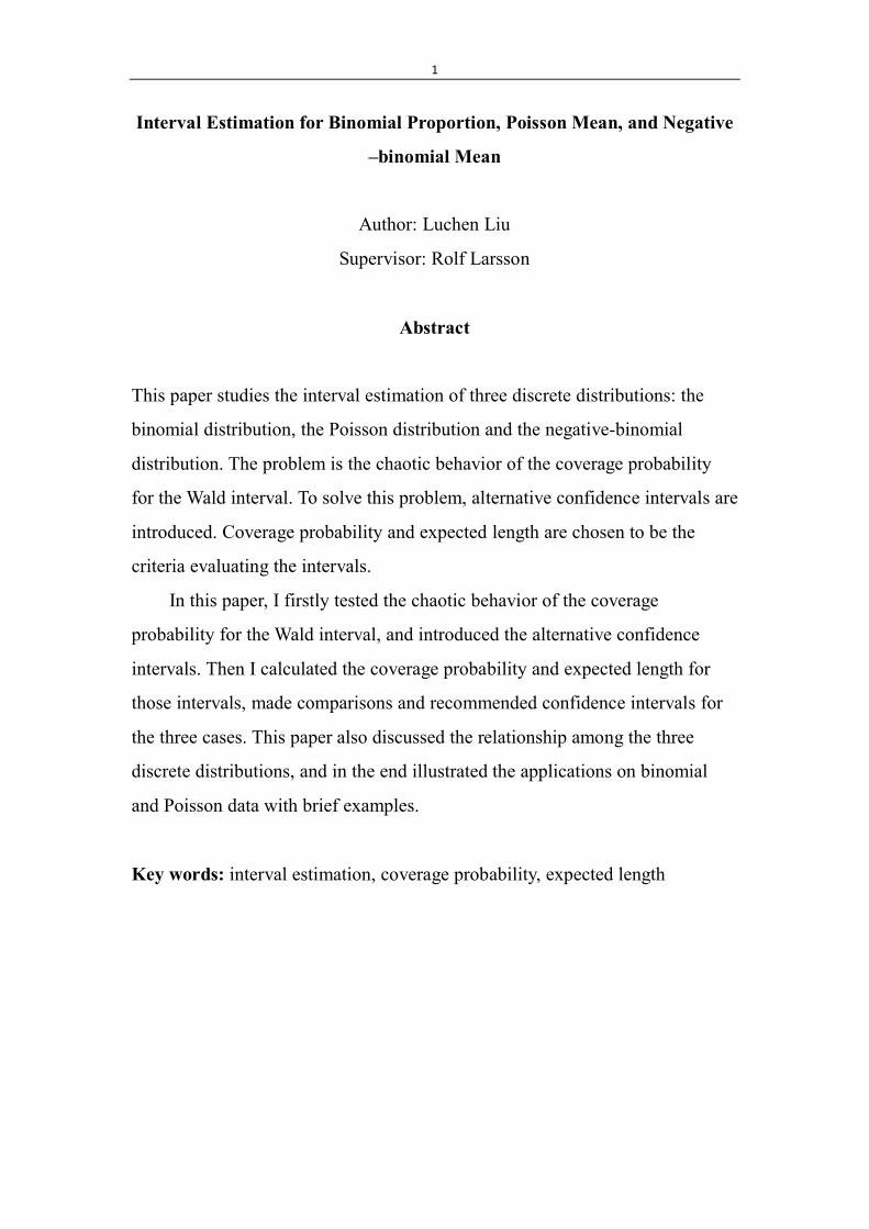
Abstract

This paper studies the interval estimation of three discrete distributions: the

binomial distribution, the Poisson distribution and the negative-binomial

distribution. The problem is the chaotic behavior of the coverage probability

for the Wald interval. To solve this problem, alternative confidence intervals are

introduced. Coverage probability and expected length are chosen to be the

criteria evaluating the intervals.

In this paper, I firstly tested the chaotic behavior of the coverage

probability for the Wald interval, and introduced the alternative confidence

intervals. Then I calculated the coverage probability and expected length for

those intervals, made comparisons and recommended confidence intervals for

the three cases. This paper also discussed the relationship among the three

discrete distributions, and in the end illustrated the applications on binomial

and Poisson data with brief examples.

Key words: interval estimation, coverage probability, expected length

2

1. Introduction

Interval estimation is one of the most basic methodologies in statistics. There

are a variety of ways to construct confidence intervals, and the most

well-known is the Wald interval. This interval is used in the textbooks, and it is

also the most commonly used confidence interval in practice. But in the

binomial case, in some studies this interval was proved to have poor coverage

probability. Agresti and Coull (1998) and Brown et. al. (2001) all considered

this problem, and figured out that, even when n is large the chaotic behavior of

the standard interval still exists.

Many other ways of constructing intervals have been taken into

consideration recently. These intervals contain the Wilson interval (also called

the score interval), the Jeffreys equal tailed interval, the Clopper-Pearson

interval, the likelihood-ratio interval, and the Bayesian HPD interval. Agresti

and Coull (1998) recommended the confidence intervals constructed by

approximation methods because they are more efficient than the “exact”

Clopper-Pearson interval, although the exact interval is always conservative.

The confidence interval of a binomial proportion is simplest but can

illustrate many problems. In this paper, I tested the chaotic behavior of the

Wald interval of the binomial proportion, and introduced some alternative

intervals, then made a comparison of these intervals, and discussed the

relationship between some intervals. The evaluation criteria I used to compare

the confidence intervals are the coverage probability and the expected length.

To be fair in the comparison of expected length, I plotted the expected length to

the actual coverage probability but not the nominal confidence level, and got

the same conclusion as Agresti and Coull.

I also turned to the confidence interval of Poisson mean and the

Negative-binomial mean, which are two other commonly used discrete

distributions. I tested the behavior of the Wald interval, and the coverage

probability is also quite chaotic, so I tried the score interval, the likelihood ratio

interval, the exact interval, and the Jeffreys interval as the alternative intervals.

3

Then I made a comparison using the coverage probability and the expected

length as criteria, and recommended which confidence interval to choose for

these two cases. In the end I gave two empirical examples to illustrate the

applications on binomial and Poisson data.

2. Methodology

The coverage probability and the expected length are reasonable criteria for us

to find the confidence intervals that have relatively higher probability to

contain the true value and shorter length.

2.1 The Actual Coverage Probability

The coverage probability of a confidence interval is the proportion of the time

that the interval contains the true value of the parameter.

The coverage probability for a confidence interval CI of the parameter

from a distribution ~ ( | )XX f x , where ( | )Xf x is the probability density

function, is calculated by the equation

( ) ( , ) ( | )k

C I k f k

(1)

where

1, ,

( , )0, .

CII k

CI

(2)

2.2 The Expected Length

The expected length is also called the expected width, which evaluates the

accuracy of a confidence interval.

The expected length for confidence interval CI of the parameter

from a distribution ~ ( | )XX f x is calculated by the equation

( ) ( ( ) ( )) ( | )k

EW U k L k f k

(3)

where ( )U k and ( )L k are the upper and lower limits of CI.

4

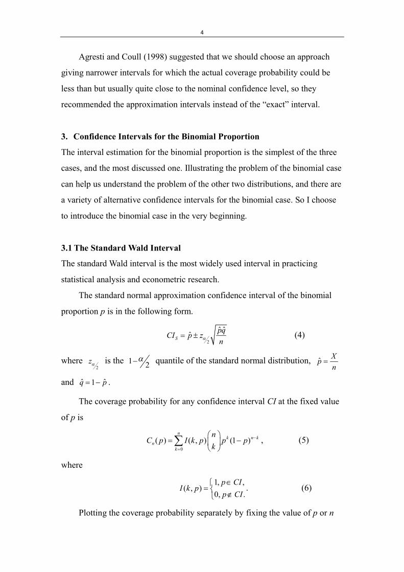
Agresti and Coull (1998) suggested that we should choose an approach

giving narrower intervals for which the actual coverage probability could be

less than but usually quite close to the nominal confidence level, so they

recommended the approximation intervals instead of the “exact” interval.

3. Confidence Intervals for the Binomial Proportion

The interval estimation for the binomial proportion is the simplest of the three

cases, and the most discussed one. Illustrating the problem of the binomial case

can help us understand the problem of the other two distributions, and there are

a variety of alternative confidence intervals for the binomial case. So I choose

to introduce the binomial case in the very beginning.

3.1 The Standard Wald Interval

The standard Wald interval is the most widely used interval in practicing

statistical analysis and econometric research.

The standard normal approximation confidence interval of the binomial

proportion p is in the following form.

2

ˆ ˆˆSpqCI p zn (4)

where 2

z is the 1 2 quantile of the standard normal distribution, ˆ Xp

n

and ˆ ˆ1q p .

The coverage probability for any confidence interval CI at the fixed value

of p is

0

( ) ( , ) (1 )n

k n kn

k

nC p I k p p p

k

, (5)

where

1, ,

( , )0, .

p CII k p

p CI

. (6)

Plotting the coverage probability separately by fixing the value of p or n

5

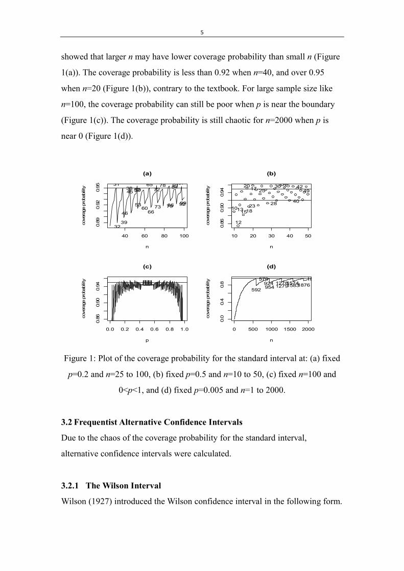
showed that larger n may have lower coverage probability than small n (Figure

1(a)). The coverage probability is less than 0.92 when n=40, and over 0.95

when n=20 (Figure 1(b)), contrary to the textbook. For large sample size like

n=100, the coverage probability can still be poor when p is near the boundary

(Figure 1(c)). The coverage probability is still chaotic for n=2000 when p is

near 0 (Figure 1(d)).

Figure 1: Plot of the coverage probability for the standard interval at: (a) fixed

p=0.2 and n=25 to 100, (b) fixed p=0.5 and n=10 to 50, (c) fixed n=100 and

0<p<1, and (d) fixed p=0.005 and n=1 to 2000.

3.2 Frequentist Alternative Confidence Intervals

Due to the chaos of the coverage probability for the standard interval,

alternative confidence intervals were calculated.

3.2.1 The Wilson Interval

Wilson (1927) introduced the Wilson confidence interval in the following form.

40 60 80 100

0.89

0.92

0.95

(a)

n

cove

rage

pro

babi

lity

25

31

32

38

39

45

46

52

53

59

60

65

66

72

73

78

79

84

86

91

92

97

99

10 20 30 40 50

0.86

0.90

0.94

(b)

n

cove

rage

pro

babi

lity

10

12

1315

17

18

20

23

25

28

30 3537

40

4249

0.0 0.2 0.4 0.6 0.8 1.0

0.86

0.90

0.94

(c)

p

cove

rage

pro

babi

lity

0 500 1000 1500 2000

0.0

0.4

0.8

(d)

n

cove

rage

pro

babi

lity 579

592924954

12781279

15741583

18561875

1876

6

21

22212 22

2 2

2 2

2 ˆ ˆ( )(4 )W

zz n zX

CI pq nn z n z

(7)

The Wilson interval is the inversion of the equal-tail test 0 0:H p p based on

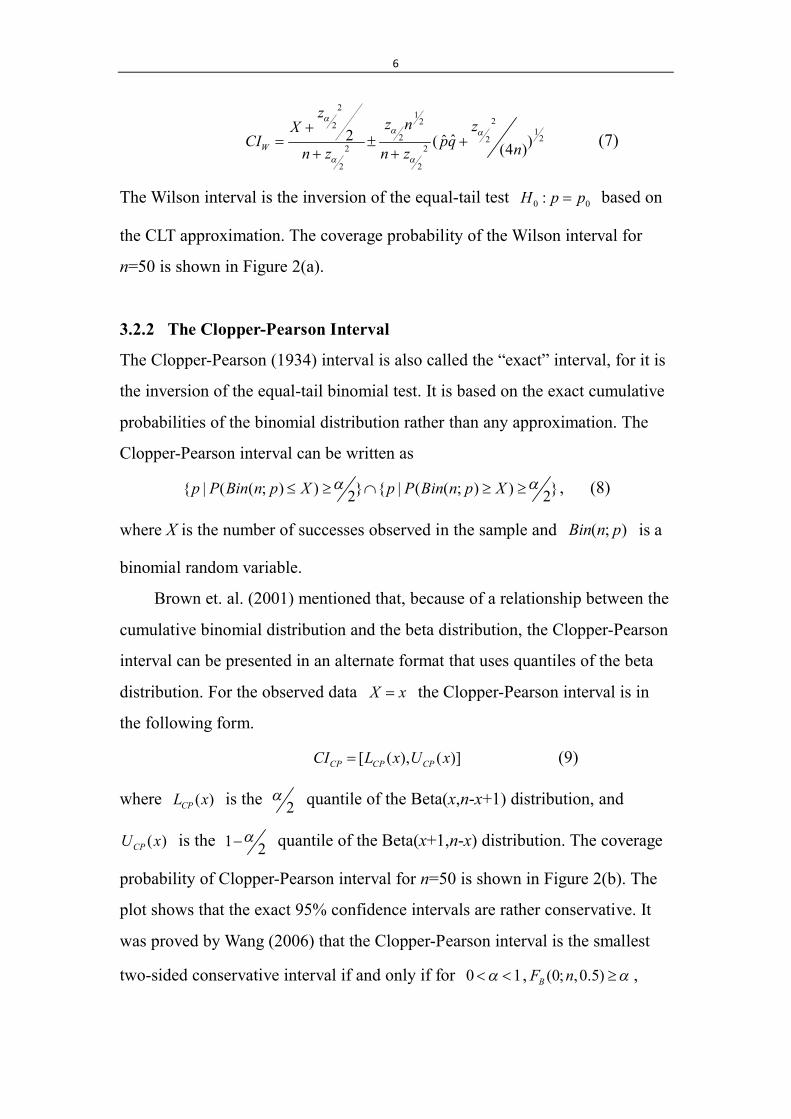
the CLT approximation. The coverage probability of the Wilson interval for

n=50 is shown in Figure 2(a).

3.2.2 The Clopper-Pearson Interval

The Clopper-Pearson (1934) interval is also called the “exact” interval, for it is

the inversion of the equal-tail binomial test. It is based on the exact cumulative

probabilities of the binomial distribution rather than any approximation. The

Clopper-Pearson interval can be written as

{ | ( ( ; ) ) } { | ( ( ; ) ) }2 2p P Bin n p X p P Bin n p X , (8)

where X is the number of successes observed in the sample and ( ; )Bin n p is a

binomial random variable.

Brown et. al. (2001) mentioned that, because of a relationship between the

cumulative binomial distribution and the beta distribution, the Clopper-Pearson

interval can be presented in an alternate format that uses quantiles of the beta

distribution. For the observed data X x the Clopper-Pearson interval is in

the following form.

[ ( ), ( )]CP CP CPCI L x U x (9)

where ( )CPL x is the 2 quantile of the Beta(x,n-x+1) distribution, and

( )CPU x is the 1 2 quantile of the Beta(x+1,n-x) distribution. The coverage

probability of Clopper-Pearson interval for n=50 is shown in Figure 2(b). The

plot shows that the exact 95% confidence intervals are rather conservative. It

was proved by Wang (2006) that the Clopper-Pearson interval is the smallest

two-sided conservative interval if and only if for 0 1 , (0; ,0.5)BF n ,

7

where ( ; , )BF x n p is the cumulative distribution function of the binomial

distribution.

3.2.3 The Agresti-Coull Interval

Agresti and Coull (1998) pointed out that the Clopper-Pearson interval is

inefficient, and suggested an adjusted Wald interval in the following form.

2

ACpqCI p zn

(10)

where 2

22

zX X

and 2

2n n z , then Xp n

and 1q p . The

coverage probability of Agresti-Coull interval for n=50 is shown in Figure 2(c).

For a 95% confidence interval, 2 2

21.96 3.84 4z , so if we use 2 instead of

1.96, this is an “add 2 successes and 2 failures” interval.

The standard interval is simple for classroom presentation, but

unfortunately with poor performance. This interval was suggested by Agresti

and Coull (1998) for that, it is of the familiar form with 2

ˆ ˆˆ pqp zn , and thus

a compromise alternative interval for the Wald interval.

3.2.4 The Likelihood Ratio Interval

The likelihood ratio interval was carried out by Rao (1973), and it is

constructed by the inversion of the likelihood ratio test 0 0:H p p if

2

22log( )n z , where n is the likelihood ratio in the following form.

0 0 0( ) (1 )( ) ( ) (1 )

X n X

n X n Xp

L p p pX XSup L p n n

(11)

where ( )L is the likelihood function. The coverage probability of the

likelihood ratio interval for n=50 is shown in Figure 2(d). We can see from the

plot that the coverage probability gets quite chaotic when p is close to the

8

boundary, but when 0.2<p<0.8 the coverage probability fluctuates around 0.95.

Figure 2: Plot of the coverage probability for n=50, 0.5 and 0<p<1 of: (a)

the Wilson interval, (b) the Clopper-Pearson interval, (c) the Agresti-Coull

interval, and (d) the likelihood ratio interval.

3.3 The Bayesian Alternative Confidence Interval

3.3.1 Jeffreys Interval

The conjugate priors of the binomial distribution are the Beta distributions, that

is to say, if the prior is ~ ( , )p Beta a b , then the posterior distribution of p is

~ ( , )p X Beta X a n X b , so the equal-tailed Bayesian interval is in the

following form.

[ ( ), ( )]B B BCI L x U x (12)

where ( )BL x is the 2 quantile and ( )BU x is the 1 2

quantile of the

( , )Beta X a n X b distribution.

The non-informative Jeffreys prior of the binomial distribution is

0.0 0.2 0.4 0.6 0.8 1.0

0.80

0.85

0.90

0.95

1.00

(a)

p

cove

rage

pro

babi

lity

0.0 0.2 0.4 0.6 0.8 1.0

0.80

0.85

0.90

0.95

1.00

(b)

p

cove

rage

pro

babi

lity

0.0 0.2 0.4 0.6 0.8 1.0

0.80

0.85

0.90

0.95

1.00

(c)

p

cove

rage

pro

babi

lity

0.0 0.2 0.4 0.6 0.8 1.0

0.80

0.85

0.90

0.95

1.00

(d)

p

cove

rage

pro

babi

lity

9

1 1( , )2 2Beta , thus the equal-tailed Jeffreys prior interval is in the following

form.

[ ( ), ( )]J J JCI L x U x (13)

where ( )JL x is the 2 quantile and ( )JU x is the 1 2

quantile of the

1 1( , )2 2Beta X n X distribution. The coverage probability of Jeffreys

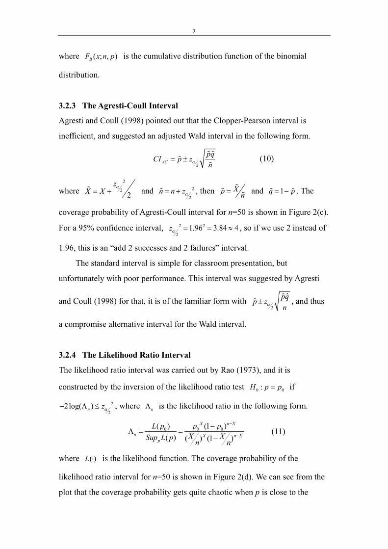
interval for n=50 is shown in Figure 3(a).

As the upper limit of the Clopper-Pearson interval is the 2 quantile of

the Beta(x,n-x+1) distribution, and the lower limit is 1 2 quantile of the

Beta(x+1,n-x) distribution, it is pointed out by Brown et. al. (2001) that Jeffreys

interval is always contained in the exact interval, thus corrects the

conservativeness of the exact interval.

3.3.2 The Bayesian HPD Interval

The highest posterior density (HPD) region consists of p that fulfill ( | )f p x c

where ( | )f p x is the posterior density of p. The highest posterior density

(HPD) interval can be denoted as:

2ˆ ˆ( ) { :[ ( ) ( ) ( ) ( )] }H b p P l p l p h p h p b , (14)

where ( )l is the log-likelihood function, and ( )h p is the prior of p (Severini,

1991). The coverage probability of the Bayesian HPD Interval for n=50 with

1 1( , )2 2Beta prior is shown in Figure 3(b). We can see from the plot that the

coverage probability gets quite chaotic when p is close to the boundary, but

when 0.2<p<0.8 the coverage probability gets less oscillation and fluctuates

around 0.95, which is with the same shape as the likelihood ratio interval.

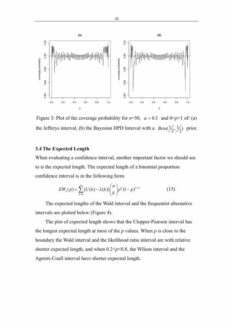
10

Figure 3: Plot of the coverage probability for n=50, 0.5 and 0<p<1 of: (a)

the Jefferys interval, (b) the Bayesian HPD Interval with a 1 1( , )2 2Beta prior.

3.4 The Expected Length

When evaluating a confidence interval, another important factor we should see

to is the expected length. The expected length of a binomial proportion

confidence interval is in the following form.

0( ) ( ( ) ( )) (1 )

nk n k

nk

nEW p U k L k p p

k

(15)

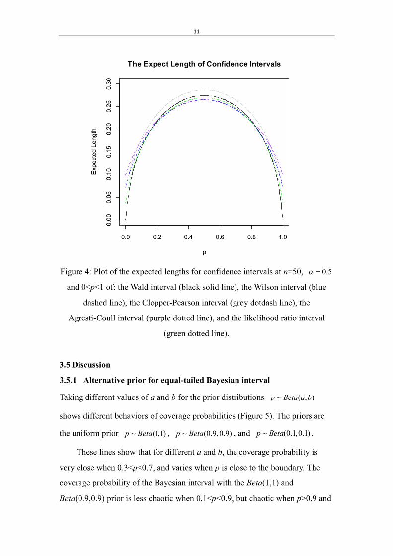
The expected lengths of the Wald interval and the frequentist alternative

intervals are plotted below (Figure 4).

The plot of expected length shows that the Clopper-Pearson interval has

the longest expected length at most of the p values. When p is close to the

boundary the Wald interval and the likelihood ratio interval are with relative

shorter expected length, and when 0.2<p<0.8, the Wilson interval and the

Agresti-Coull interval have shorter expected length.

0.0 0.2 0.4 0.6 0.8 1.0

0.80

0.85

0.90

0.95

1.00

(a)

p

cove

rage

pro

babi

lity

0.0 0.2 0.4 0.6 0.8 1.0

0.80

0.85

0.90

0.95

1.00

(b)

p

cove

rage

pro

babi

lity

11

Figure 4: Plot of the expected lengths for confidence intervals at n=50, 0.5

and 0<p<1 of: the Wald interval (black solid line), the Wilson interval (blue

dashed line), the Clopper-Pearson interval (grey dotdash line), the

Agresti-Coull interval (purple dotted line), and the likelihood ratio interval

(green dotted line).

3.5 Discussion

3.5.1 Alternative prior for equal-tailed Bayesian interval

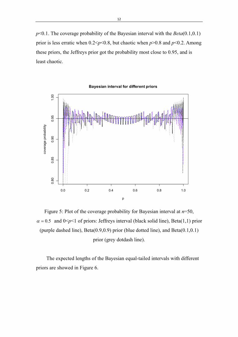
Taking different values of a and b for the prior distributions ~ ( , )p Beta a b

shows different behaviors of coverage probabilities (Figure 5). The priors are

the uniform prior ~ (1,1)p Beta , ~ (0.9,0.9)p Beta , and ~ (0.1,0.1)p Beta .

These lines show that for different a and b, the coverage probability is

very close when 0.3<p<0.7, and varies when p is close to the boundary. The

coverage probability of the Bayesian interval with the Beta(1,1) and

Beta(0.9,0.9) prior is less chaotic when 0.1<p<0.9, but chaotic when p>0.9 and

0.0 0.2 0.4 0.6 0.8 1.0

0.00

0.05

0.10

0.15

0.20

0.25

0.30

The Expect Length of Confidence Intervals

p

Exp

ecte

d Le

ngth

12

p<0.1. The coverage probability of the Bayesian interval with the Beta(0.1,0.1)

prior is less erratic when 0.2<p<0.8, but chaotic when p>0.8 and p<0.2. Among

these priors, the Jeffreys prior got the probability most close to 0.95, and is

least chaotic.

Figure 5: Plot of the coverage probability for Bayesian interval at n=50,

0.5 and 0<p<1 of priors: Jeffreys interval (black solid line), Beta(1,1) prior

(purple dashed line), Beta(0.9,0.9) prior (blue dotted line), and Beta(0.1,0.1)

prior (grey dotdash line).

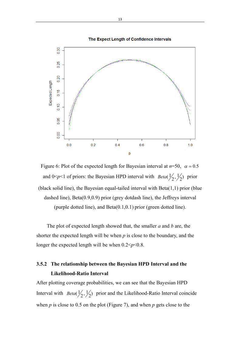
The expected lengths of the Bayesian equal-tailed intervals with different

priors are showed in Figure 6.

0.0 0.2 0.4 0.6 0.8 1.0

0.80

0.85

0.90

0.95

1.00

Bayesian interval for different priors

p

cove

rage

pro

babi

lity

13

Figure 6: Plot of the expected length for Bayesian interval at n=50, 0.5

and 0<p<1 of priors: the Bayesian HPD interval with 1 1( , )2 2Beta prior

(black solid line), the Bayesian equal-tailed interval with Beta(1,1) prior (blue

dashed line), Beta(0.9,0.9) prior (grey dotdash line), the Jeffreys interval

(purple dotted line), and Beta(0.1,0.1) prior (green dotted line).

The plot of expected length showed that, the smaller a and b are, the

shorter the expected length will be when p is close to the boundary, and the

longer the expected length will be when 0.2<p<0.8.

3.5.2 The relationship between the Bayesian HPD Interval and the

Likelihood-Ratio Interval

After plotting coverage probabilities, we can see that the Bayesian HPD

Interval with 1 1( , )2 2Beta prior and the Likelihood-Ratio Interval coincide

when p is close to 0.5 on the plot (Figure 7), and when p gets close to the

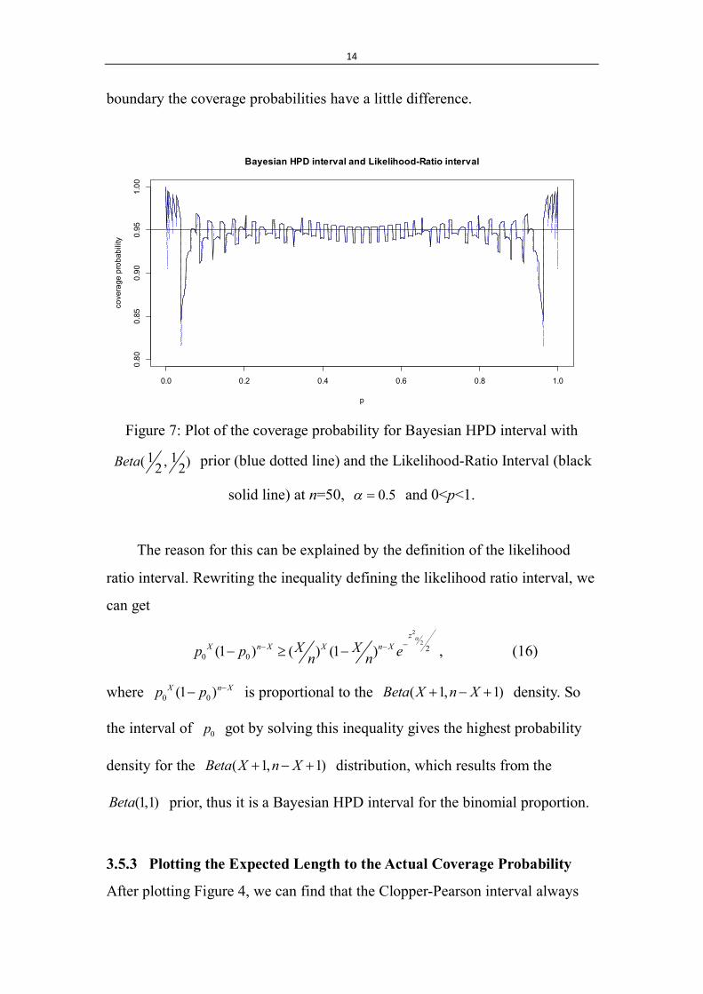
14

boundary the coverage probabilities have a little difference.

Figure 7: Plot of the coverage probability for Bayesian HPD interval with

1 1( , )2 2Beta prior (blue dotted line) and the Likelihood-Ratio Interval (black

solid line) at n=50, 0.5 and 0<p<1.

The reason for this can be explained by the definition of the likelihood

ratio interval. Rewriting the inequality defining the likelihood ratio interval, we

can get 2

22

0 0(1 ) ( ) (1 )z

X n X X n XX Xp p en n

, (16)

where 0 0(1 )X n Xp p is proportional to the ( 1, 1)Beta X n X density. So

the interval of 0p got by solving this inequality gives the highest probability

density for the ( 1, 1)Beta X n X distribution, which results from the

(1,1)Beta prior, thus it is a Bayesian HPD interval for the binomial proportion.

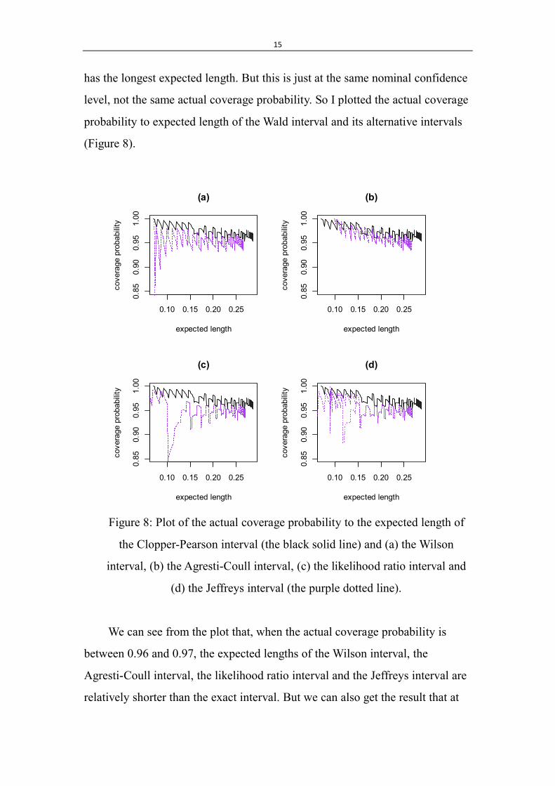
3.5.3 Plotting the Expected Length to the Actual Coverage Probability

After plotting Figure 4, we can find that the Clopper-Pearson interval always

0.0 0.2 0.4 0.6 0.8 1.0

0.80

0.85

0.90

0.95

1.00

Bayesian HPD interval and Likelihood-Ratio interval

p

cove

rage

pro

babi

lity

15

has the longest expected length. But this is just at the same nominal confidence

level, not the same actual coverage probability. So I plotted the actual coverage

probability to expected length of the Wald interval and its alternative intervals

(Figure 8).

Figure 8: Plot of the actual coverage probability to the expected length of

the Clopper-Pearson interval (the black solid line) and (a) the Wilson

interval, (b) the Agresti-Coull interval, (c) the likelihood ratio interval and

(d) the Jeffreys interval (the purple dotted line).

We can see from the plot that, when the actual coverage probability is

between 0.96 and 0.97, the expected lengths of the Wilson interval, the

Agresti-Coull interval, the likelihood ratio interval and the Jeffreys interval are

relatively shorter than the exact interval. But we can also get the result that at

0.10 0.15 0.20 0.25

0.85

0.90

0.95

1.00

(a)

expected length

cove

rage

pro

babi

lity

0.10 0.15 0.20 0.250.

850.

900.

951.

00

(b)

expected length

cove

rage

pro

babi

lity

0.10 0.15 0.20 0.25

0.85

0.90

0.95

1.00

(c)

expected length

cove

rage

pro

babi

lity

0.10 0.15 0.20 0.25

0.85

0.90

0.95

1.00

(d)

expected length

cove

rage

pro

babi

lity

16

the same expected length, the Clopper-Pearson interval always has the largest

actual coverage probability. So it is not proper to say that the Clopper-Pearson

interval is inefficient, because the expected length of the Agresti-Coull interval

and the Clopper-Pearson interval at the same actual coverage probability are

not very different at the same nominal confidence level.

So I think we should choose the confidence interval for the binomial

proportion according to the requirement and the purpose of the study. If we are

doing analysis requiring conservativeness of the confidence interval, we should

choose the exact interval, and if we want to obtain a more accurate interval, we

should choose the Agresti-Coull interval instead.

4. The Confidence Interval for the Poisson Mean

The Poisson distribution is another discrete distribution in the exponential

family. The estimation of the Poisson mean is also a commonly discussed

problem in statistical analysis. The Poisson distribution describes the

probability of a given number of events occurring in a fixed interval of time or

space if those events occur with a known average rate and independently of the

time since the last event. Let 1{ , , }nX X be independent, identically

distributed ( )Poisson random variables, then the probability density function

of iX is

( )!

k

ieP X kk

(17)

where k is a non-negative integer, and is a positive real number, which

equals the expectation of X.

4.1 The Wald Interval

The simplest and most widely used confidence interval for a Poisson mean is

still the Wald interval.

For an independent, identically distributed ( )Poisson random sample

17

1{ , , }nX X , the standard normal approximation confidence interval of the

Poisson mean is in the following form. 1

2

2( )XX z n (18)

where 1

n

ii

X X n

, and 2

z is the 1 2 quantile of the standard normal

distribution.

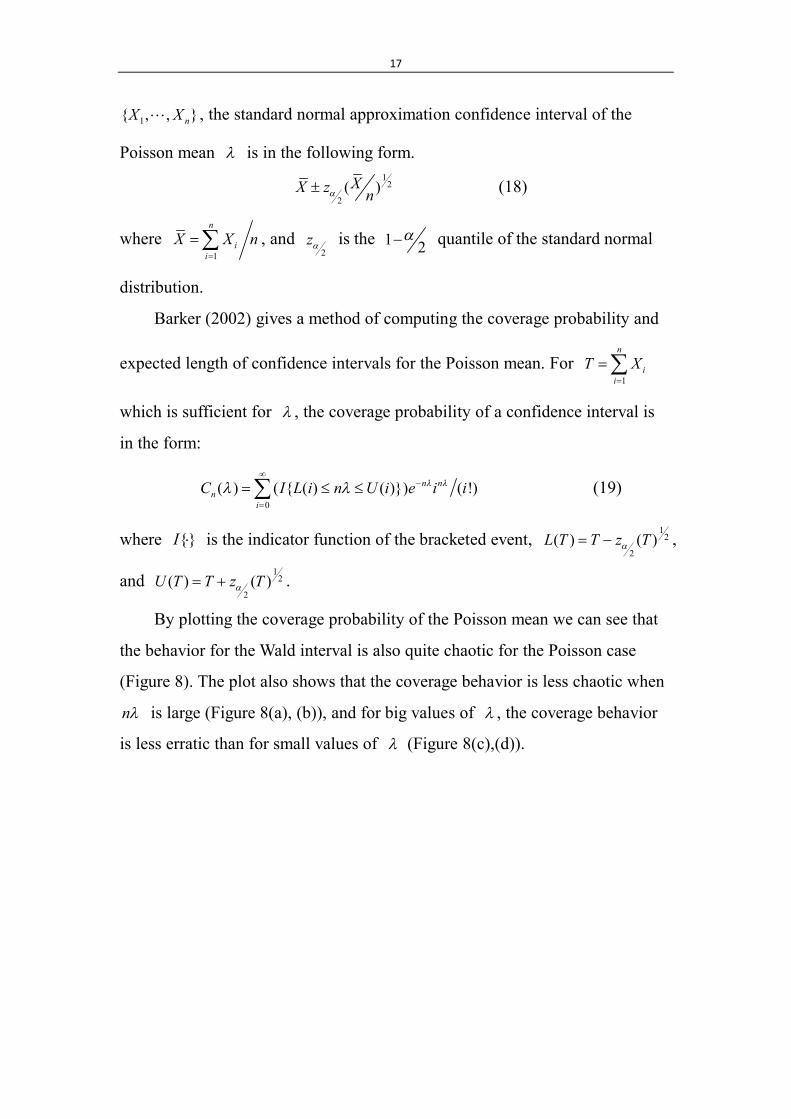
Barker (2002) gives a method of computing the coverage probability and

expected length of confidence intervals for the Poisson mean. For 1

n

ii

T X

which is sufficient for , the coverage probability of a confidence interval is

in the form:

0( ) ( { ( ) ( )}) ( !)n n

ni

C I L i n U i e i i

(19)

where {}I is the indicator function of the bracketed event, 1

2

2( ) ( )L T T z T ,

and 1

2

2( ) ( )U T T z T .

By plotting the coverage probability of the Poisson mean we can see that

the behavior for the Wald interval is also quite chaotic for the Poisson case

(Figure 8). The plot also shows that the coverage behavior is less chaotic when

n is large (Figure 8(a), (b)), and for big values of , the coverage behavior

is less erratic than for small values of (Figure 8(c),(d)).

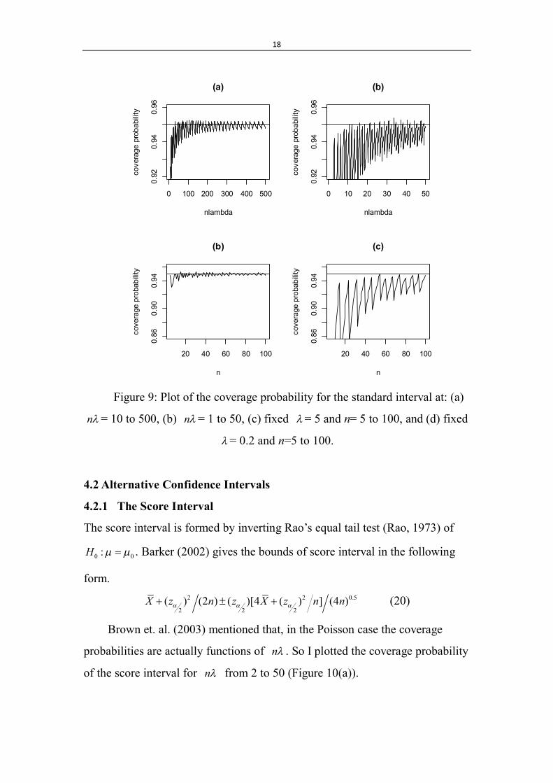
18

Figure 9: Plot of the coverage probability for the standard interval at: (a)

n = 10 to 500, (b) n = 1 to 50, (c) fixed = 5 and n= 5 to 100, and (d) fixed

= 0.2 and n=5 to 100.

4.2 Alternative Confidence Intervals

4.2.1 The Score Interval

The score interval is formed by inverting Rao’s equal tail test (Rao, 1973) of

0 0:H . Barker (2002) gives the bounds of score interval in the following

form. 2 2 0.5

2 2 2( ) (2 ) ( )[4 ( ) ] (4 )X z n z X z n n (20)

Brown et. al. (2003) mentioned that, in the Poisson case the coverage

probabilities are actually functions of n . So I plotted the coverage probability

of the score interval for n from 2 to 50 (Figure 10(a)).

0 100 200 300 400 500

0.92

0.94

0.96

(a)

nlambda

cove

rage

pro

babi

lity

0 10 20 30 40 50

0.92

0.94

0.96

(b)

nlambda

cove

rage

pro

babi

lity

20 40 60 80 100

0.86

0.90

0.94

(b)

n

cove

rage

pro

babi

lity

20 40 60 80 100

0.86

0.90

0.94

(c)

n

cove

rage

pro

babi

lity

19

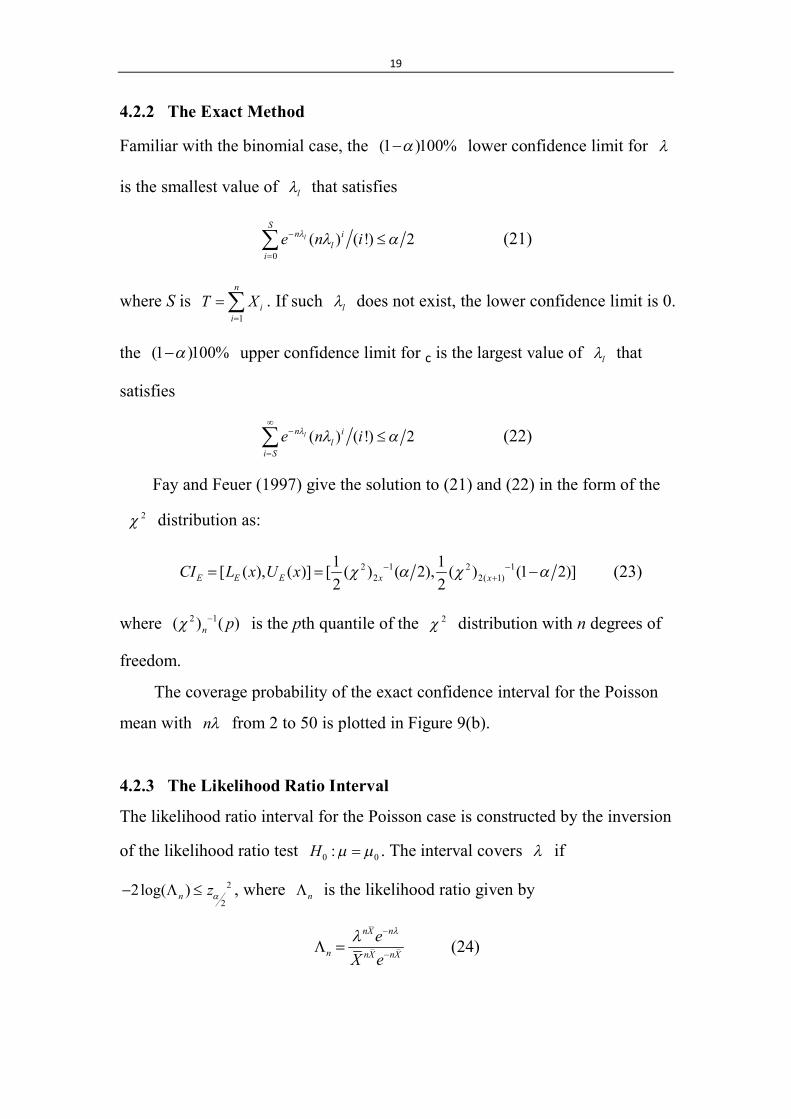
4.2.2 The Exact Method

Familiar with the binomial case, the (1 )100% lower confidence limit for

is the smallest value of l that satisfies

0( ) ( !) 2l

Sn i

li

e n i

(21)

where S is 1

n

ii

T X

. If such l does not exist, the lower confidence limit is 0.

the (1 )100% upper confidence limit for c is the largest value of l that

satisfies

( ) ( !) 2ln il

i Se n i

(22)

Fay and Feuer (1997) give the solution to (21) and (22) in the form of the

2 distribution as:

2 1 2 12 2( 1)

1 1[ ( ), ( )] [ ( ) ( 2), ( ) (1 2)]2 2E E E x xCI L x U x

(23)

where 2 1( ) ( )n p is the pth quantile of the 2 distribution with n degrees of

freedom.

The coverage probability of the exact confidence interval for the Poisson

mean with n from 2 to 50 is plotted in Figure 9(b).


The likelihood ratio interval for the Poisson case is constructed by the inversion

of the likelihood ratio test 0 0:H . The interval covers if

2

22log( )n z , where n is the likelihood ratio given by

nX n

n nX nX

eX e

(24)

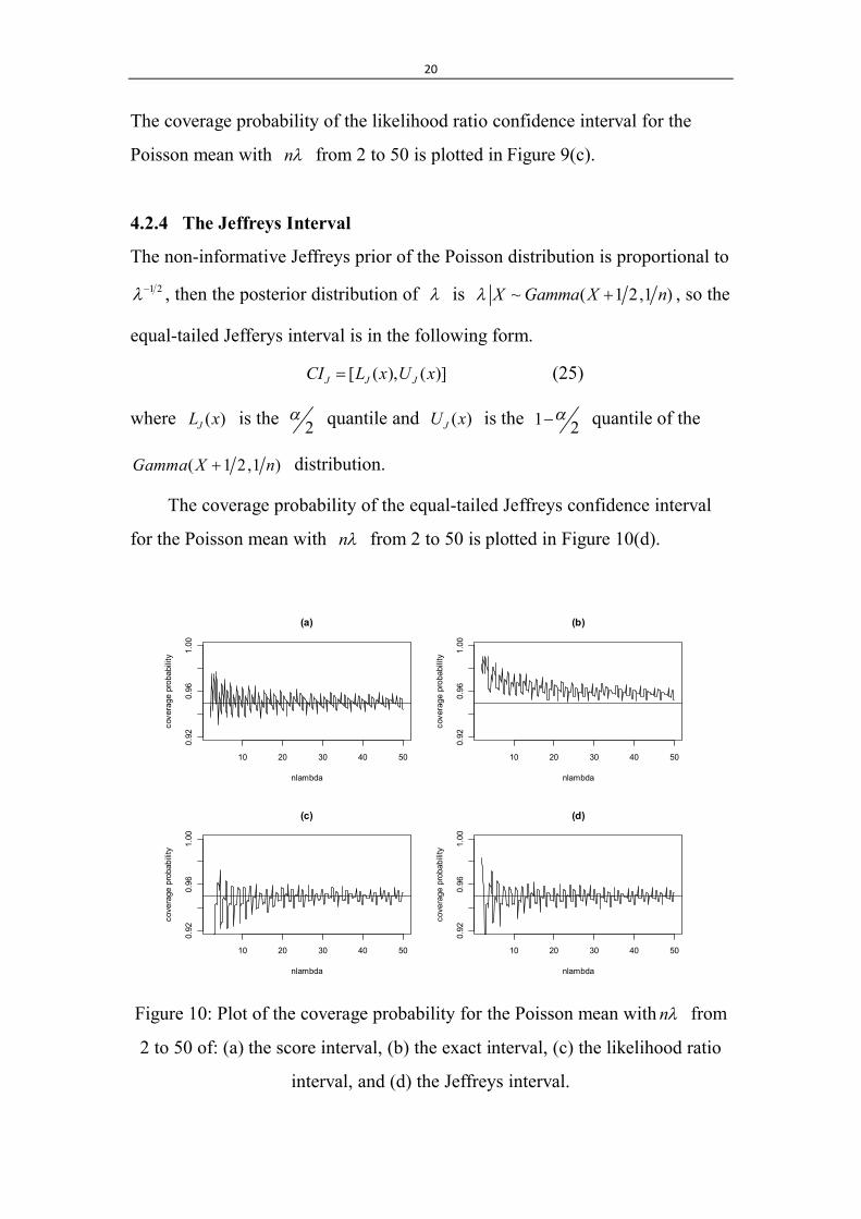
20

The coverage probability of the likelihood ratio confidence interval for the

Poisson mean with n from 2 to 50 is plotted in Figure 9(c).

4.2.4 The Jeffreys Interval

The non-informative Jeffreys prior of the Poisson distribution is proportional to 1 2 , then the posterior distribution of is ~ ( 1 2,1 )X Gamma X n , so the

equal-tailed Jefferys interval is in the following form.

[ ( ), ( )]J J JCI L x U x (25)


quantile of the

( 1 2,1 )Gamma X n distribution.

The coverage probability of the equal-tailed Jeffreys confidence interval

for the Poisson mean with n from 2 to 50 is plotted in Figure 10(d).

Figure 10: Plot of the coverage probability for the Poisson mean with n from

2 to 50 of: (a) the score interval, (b) the exact interval, (c) the likelihood ratio

interval, and (d) the Jeffreys interval.

10 20 30 40 50

0.92

0.96

1.00

(a)

nlambda

cove

rage

pro

babi

lity

10 20 30 40 50

0.92

0.96

1.00

(b)

nlambda

cove

rage

pro

babi

lity

10 20 30 40 50

0.92

0.96

1.00

(c)

nlambda

cove

rage

pro

babi

lity

10 20 30 40 50

0.92

0.96

1.00

(d)

nlambda

cove

rage

pro

babi

lity

21

From the plots we can see that the likelihood ratio interval and the Jeffreys

interval are more chaotic than the score interval and the exact interval, and the

exact interval is the most conservative interval among these four intervals.

The likelihood ratio interval and the Jeffreys interval in the Poisson case

are also close to each other when n is large. As in the binomial case, when

n is close to the boundary 0, the coverage probabilities are slightly different.

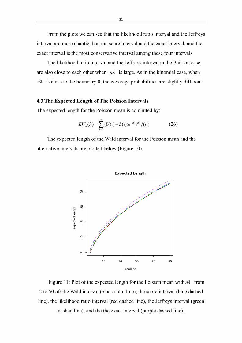
4.3 The Expected Length of The Poisson Intervals

The expected length for the Poisson mean is computed by:

0

( ) ( ( ) ( )) ( !)n nn

iEW U i L i e i i

(26)

The expected length of the Wald interval for the Poisson mean and the

alternative intervals are plotted below (Figure 10).

Figure 11: Plot of the expected length for the Poisson mean with n from

2 to 50 of: the Wald interval (black solid line), the score interval (blue dashed

line), the likelihood ratio interval (red dashed line), the Jeffreys interval (green

dashed line), and the the exact interval (purple dashed line).

10 20 30 40 50

510

1520

25

Expected Length

nlambda

expe

cted

leng

th

22

We can see from the plot that the expected lengths of the Wald interval

and the likelihood ratio interval are the shortest, the expected length of the

Jeffreys interval is close to the Wald interval, the expected length of the score

interval is a little bit longer, and the exact interval is the longest.

Then we can also plot the expected length to the actual coverage

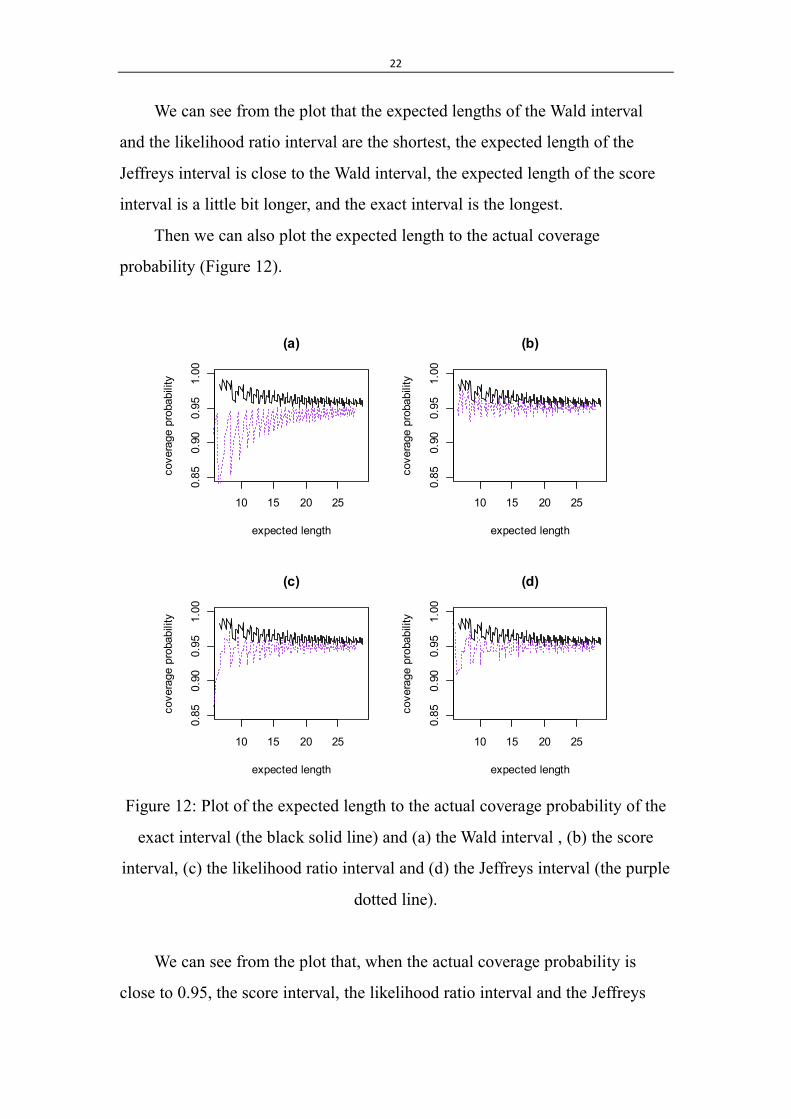
probability (Figure 12).

Figure 12: Plot of the expected length to the actual coverage probability of the

exact interval (the black solid line) and (a) the Wald interval , (b) the score

interval, (c) the likelihood ratio interval and (d) the Jeffreys interval (the purple

dotted line).


close to 0.95, the score interval, the likelihood ratio interval and the Jeffreys

10 15 20 25

0.85

0.90

0.95

1.00

(a)

expected length

cove

rage

pro

babi

lity

10 15 20 25

0.85

0.90

0.95

1.00

(b)

expected length

cove

rage

pro

babi

lity

10 15 20 25

0.85

0.90

0.95

1.00

(c)

expected length

cove

rage

pro

babi

lity

10 15 20 25

0.85

0.90

0.95

1.00

(d)

expected length

cove

rage

pro

babi

lity

23

interval are relatively shorter than the exact interval. And we can also see that

at the same expected length, the actual coverage probability of the exact

interval is always the largest.

So we should also choose the confidence interval like in the binomial case.

The approximation methods are more accurate but with smaller coverage

probability, thus are proper to be used in the studies requiring efficiency. The

exact method should be used if the study requires conservativeness.

5. The Confidence Interval for the Negative binomial Mean

The probability density function for the negative-binomial variable

~ ( , )X NB r p is in the form.

1( | ) (1 ) , 0,1, ;0 1r xr x

P X x p p p x px

(27)

The mean and variance are (1 )( ) r pE Xp

and 2

(1 )( ) r pVar Xp

.

The negative binomial variable ~ ( , )X NB r p can describe the number of

failures before the first r success when doing Bernoulli trials.

5.1 The Wald Interval

Let 1{ , , }nX X be independent, identically distributed (1, )NB p random

variables, then ~ (1, )X NB p and 0

~ ( , )n

ii

X NB n p .

The point estimation of the probability of success p is 1ˆ1

pX

. The

estimation of the mean is ˆ X , and the variance of the mean is 22

ˆ(1 )ˆˆ

pp

.

So the standard Wald confidence interval for the negative-binomial mean is in

the following form.

24

222 2

ˆ(1 )ˆ ˆˆS

pCI z X zp

(28)

where 2

z is the 1 2 quantile of the standard normal distribution.

The coverage probability of the confidence intervals for the

negative-binomial mean is calculated by the equation

0

1( ) ( { ( ) ( )}) (1 )r i

ri

r iCP I L i U i p p

i

0

1( { ( ) ( )}) ( ) (1 )r i

i

r i r rI L i U ii r r

(29)

where {}I is the indicator function of the bracketed event, ( )U i and ( )L i

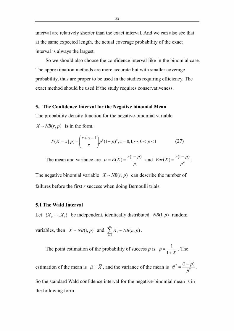
are the upper and lower bounds of the confidence interval.

The behavior of the coverage probability of the standard Wald interval for

the negative binomial mean is quite chaotic (Figure 13), and even never

reaches the nominal confidence level. For large values of n (Figure 13(d)) and

(Figure 13(b)) the coverage probability performs less chaotically than for a

small value (Figure 13(a), (c)). The coverage probability of the Wald interval

for the negative-binomial mean is in general quite chaotic as it never reaches

the nominal confidence level even when n=100. But the coverage probability

reaches 0.95 when n=1000 (Figure 17).

25

Figure 13: Plot of the coverage probability of the Wald interval for the

negative binomial mean at: (a) fixed 5 and n=2 to 50, (b) fixed 100

and n=2 to 50, (c) fixed n=20 and 0 to 100, and (d) fixed n=100 and

0 to 100.

5.2 The Alternative Confidence Intervals

5.2.1 The Score Interval

The Rao’s score interval of the negative-binomial mean given by Brown et. al.

(2003) is in the form

12 22122 2 2 2

2 2

2 2

ˆ 2ˆ ˆ( )

4R

n z z n zCI

n z n z n

(30)

10 20 30 40 50

0.5

0.7

0.9

(a)

n

cove

rage

pro

babi

lity

10 20 30 40 50

0.5

0.7

0.9

(b)

n

cove

rage

pro

babi

lity

0 20 40 60 80 100

0.5

0.7

0.9

(c)

mu

cove

rage

pro

babi

lity

0 20 40 60 80 100

0.5

0.7

0.9

(d)

mu

cove

rage

pro

babi

lity

26

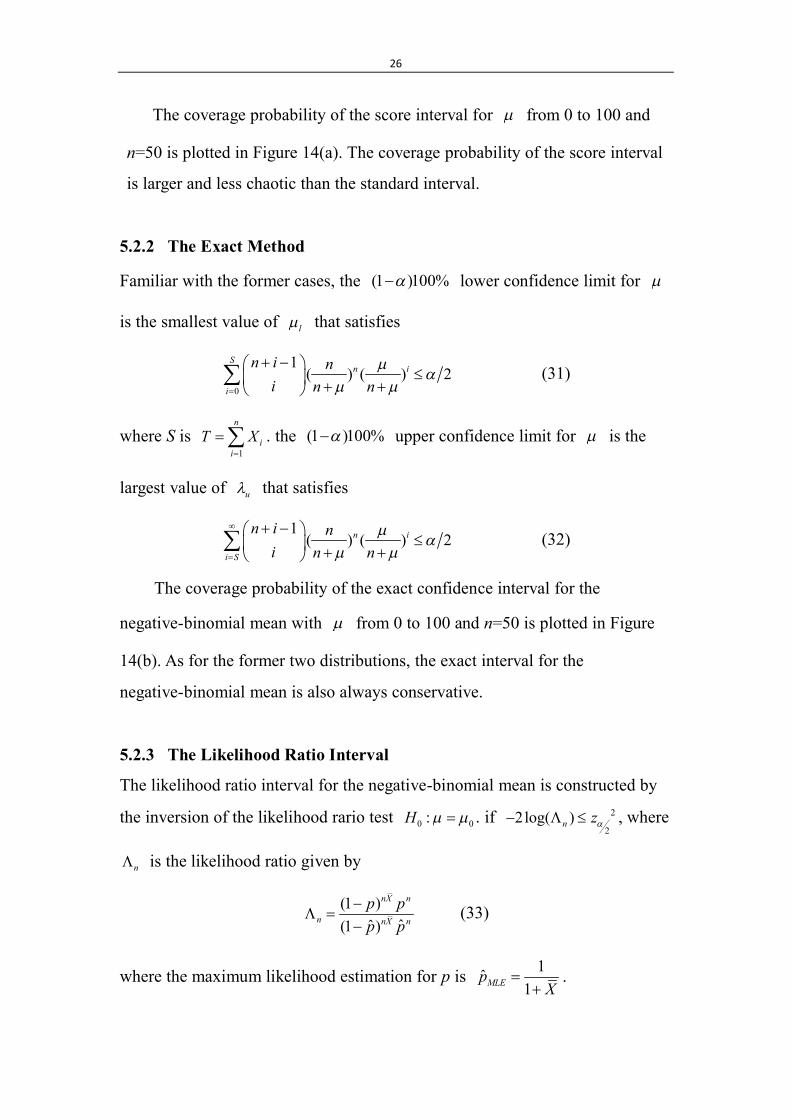
The coverage probability of the score interval for from 0 to 100 and

n=50 is plotted in Figure 14(a). The coverage probability of the score interval

is larger and less chaotic than the standard interval.

5.2.2 The Exact Method

Familiar with the former cases, the (1 )100% lower confidence limit for

is the smallest value of l that satisfies

0

1( ) ( ) 2

Sn i

i

n i ni n n

(31)

where S is 1

n

ii

T X

. the (1 )100% upper confidence limit for is the

largest value of u that satisfies

1( ) ( ) 2n i

i S

n i ni n n

(32)

The coverage probability of the exact confidence interval for the

negative-binomial mean with from 0 to 100 and n=50 is plotted in Figure

14(b). As for the former two distributions, the exact interval for the

negative-binomial mean is also always conservative.


The likelihood ratio interval for the negative-binomial mean is constructed by

the inversion of the likelihood rario test 0 0:H . if 2

22log( )n z , where

n is the likelihood ratio given by

(1 )ˆ ˆ(1 )

nX n

n nX n

p pp p

(33)

where the maximum likelihood estimation for p is 1ˆ1MLEp

X

.

27

The coverage probability of the likelihood ratio confidence interval for the


14(c).

5.2.4 The Jeffreys Interval

Because the non-informative Jeffreys prior of the negative-binomial mean is

proportional to 1 2 1 2(1 ) , the conjugate prior for p is proportional to

1 2 1(1 ) ( )p p . So the posterior distribution of p is ~ ( 1 2, )p X Beta X n ,

and the equal-tailed Jeffreys interval is in the following form.

( ) [ ( ), ( )]J J JCI p L x U x (34)


quantile of the

( 1 2 , )Beta X n distribution. Thus the Jeffreys interval for is

( ) ( )( ) [ , ]1 ( ) 1 ( )J J

JJ J

U x L xCI U x L x (35)

The coverage probability of the equal-tailed Jeffreys confidence interval


14(d).

The likelihood ratio interval and the Jeffreys interval in the

negative-binomial case are close to each other when is large, and have

difference when is close to 0, which coincides with the former two cases.

28

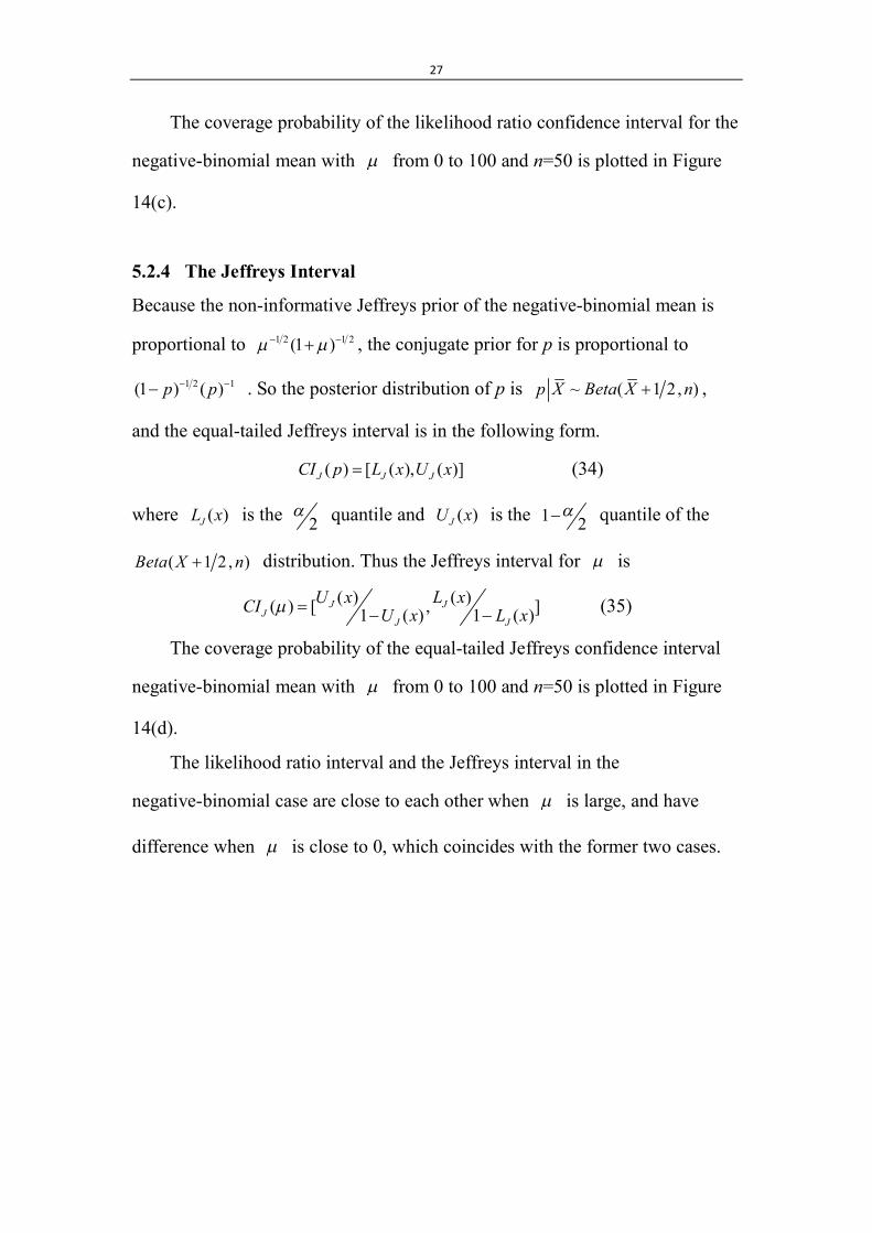
Figure 14: Plot of the coverage probability for the negative-binomial mean with

from 0 to 100 and n=50 of: (a) the score interval, (b) the exact interval, (c)

the likelihood ratio interval, and (d) the Jeffreys interval.

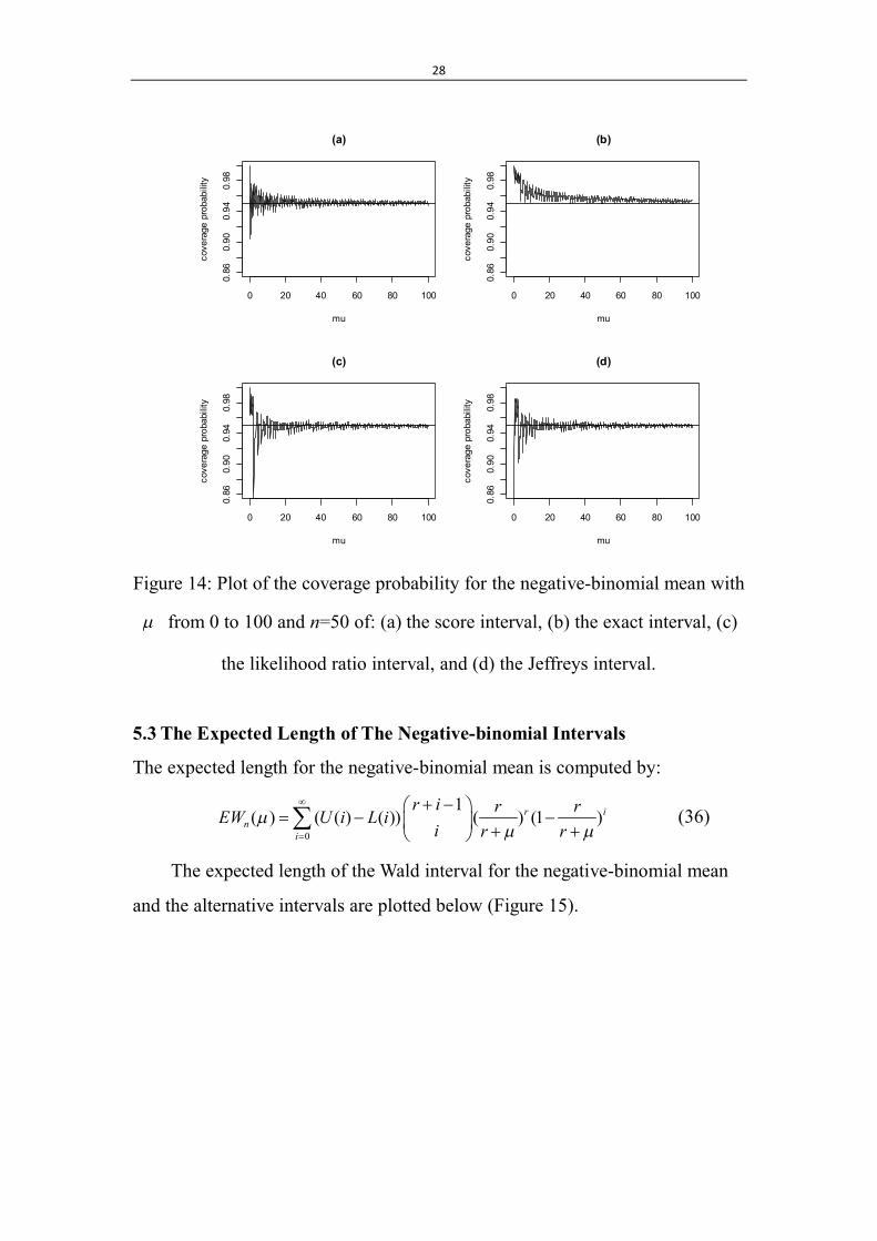
5.3 The Expected Length of The Negative-binomial Intervals

The expected length for the negative-binomial mean is computed by:

0

1( ) ( ( ) ( )) ( ) (1 )r i

ni

r i r rEW U i L ii r r

(36)

The expected length of the Wald interval for the negative-binomial mean

and the alternative intervals are plotted below (Figure 15).

0 20 40 60 80 100

0.86

0.90

0.94

0.98

(a)

mu

cove

rage

pro

babi

lity

0 20 40 60 80 100

0.86

0.90

0.94

0.98

(b)

mu

cove

rage

pro

babi

lity

0 20 40 60 80 100

0.86

0.90

0.94

0.98

(c)

mu

cove

rage

pro

babi

lity

0 20 40 60 80 100

0.86

0.90

0.94

0.98

(d)

mu

cove

rage

pro

babi

lity

29

Figure 15: Plot of the expected length for the negative-binomial with

from 0 to 100 of: the Wald interval (black solid line), the score interval (grey

dotted line), the likelihood ratio interval (green dotted line), the Jeffreys

interval (blue dotted line), and the the exact interval (red dotted line).

We can see from the plot that, the score interval has the longest expected

length most of the time, and the Wald interval is always the shortest. The

expected length of the likelihood ratio interval and the Jeffreys interval are

close to each other.

Then we can also plot the expected length to the actual coverage

probability (Figure 16)

0 20 40 60 80 100

010

2030

4050

6070

Expected Length of the Negative-binomial Mean

mu

expe

cted

leng

th

30

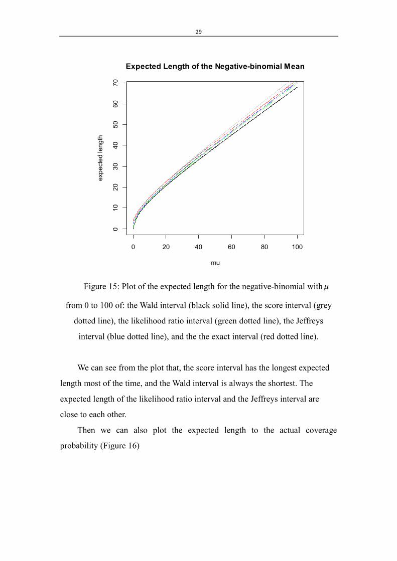
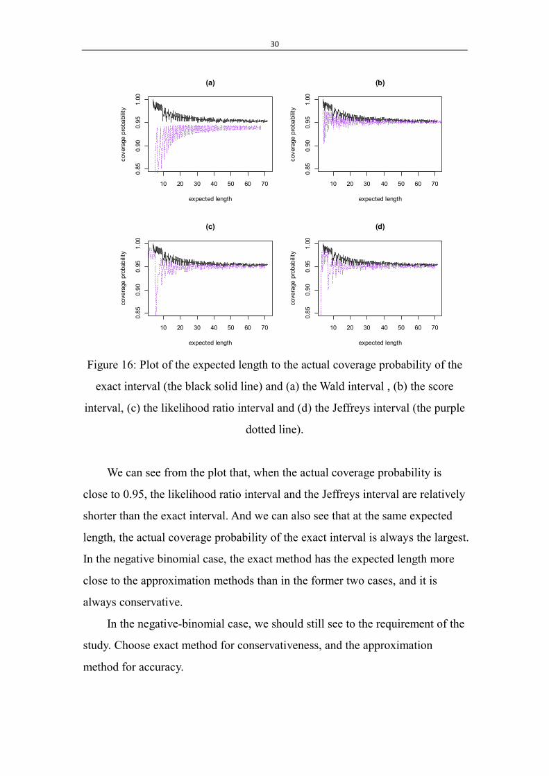
Figure 16: Plot of the expected length to the actual coverage probability of the

exact interval (the black solid line) and (a) the Wald interval , (b) the score

interval, (c) the likelihood ratio interval and (d) the Jeffreys interval (the purple

dotted line).


close to 0.95, the likelihood ratio interval and the Jeffreys interval are relatively

shorter than the exact interval. And we can also see that at the same expected

length, the actual coverage probability of the exact interval is always the largest.

In the negative binomial case, the exact method has the expected length more

close to the approximation methods than in the former two cases, and it is

always conservative.

In the negative-binomial case, we should still see to the requirement of the

study. Choose exact method for conservativeness, and the approximation

method for accuracy.

10 20 30 40 50 60 70

0.85

0.90

0.95

1.00

(a)

expected length

cove

rage

pro

babi

lity

10 20 30 40 50 60 70

0.85

0.90

0.95

1.00

(b)

expected length

cove

rage

pro

babi

lity

10 20 30 40 50 60 70

0.85

0.90

0.95

1.00

(c)

expected length

cove

rage

pro

babi

lity

10 20 30 40 50 60 70

0.85

0.90

0.95

1.00

(d)

expected length

cove

rage

pro

babi

lity

31

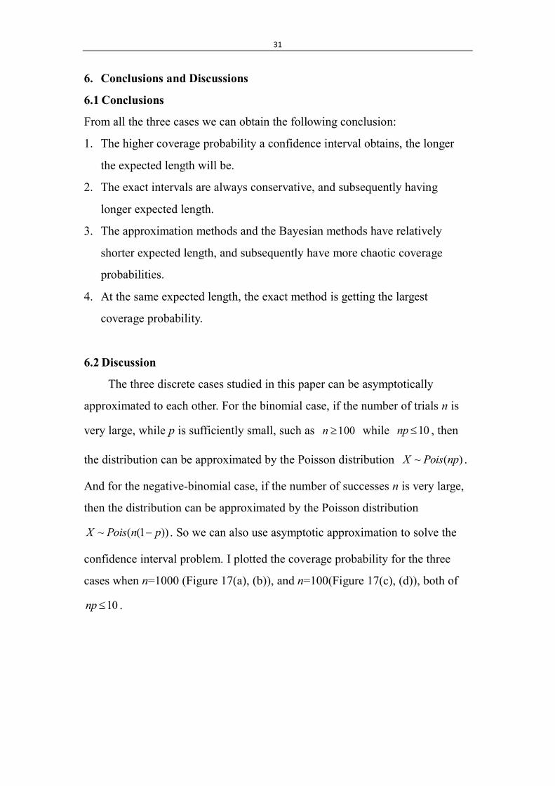
6. Conclusions and Discussions

6.1 Conclusions

From all the three cases we can obtain the following conclusion:

1. The higher coverage probability a confidence interval obtains, the longer

the expected length will be.

2. The exact intervals are always conservative, and subsequently having

longer expected length.

3. The approximation methods and the Bayesian methods have relatively

shorter expected length, and subsequently have more chaotic coverage

probabilities.

4. At the same expected length, the exact method is getting the largest

coverage probability.

6.2 Discussion

The three discrete cases studied in this paper can be asymptotically

approximated to each other. For the binomial case, if the number of trials n is

very large, while p is sufficiently small, such as 100n while 10np , then

the distribution can be approximated by the Poisson distribution ~ ( )X Pois np .

And for the negative-binomial case, if the number of successes n is very large,

then the distribution can be approximated by the Poisson distribution

~ ( (1 ))X Pois n p . So we can also use asymptotic approximation to solve the

confidence interval problem. I plotted the coverage probability for the three

cases when n=1000 (Figure 17(a), (b)), and n=100(Figure 17(c), (d)), both of

10np .

32

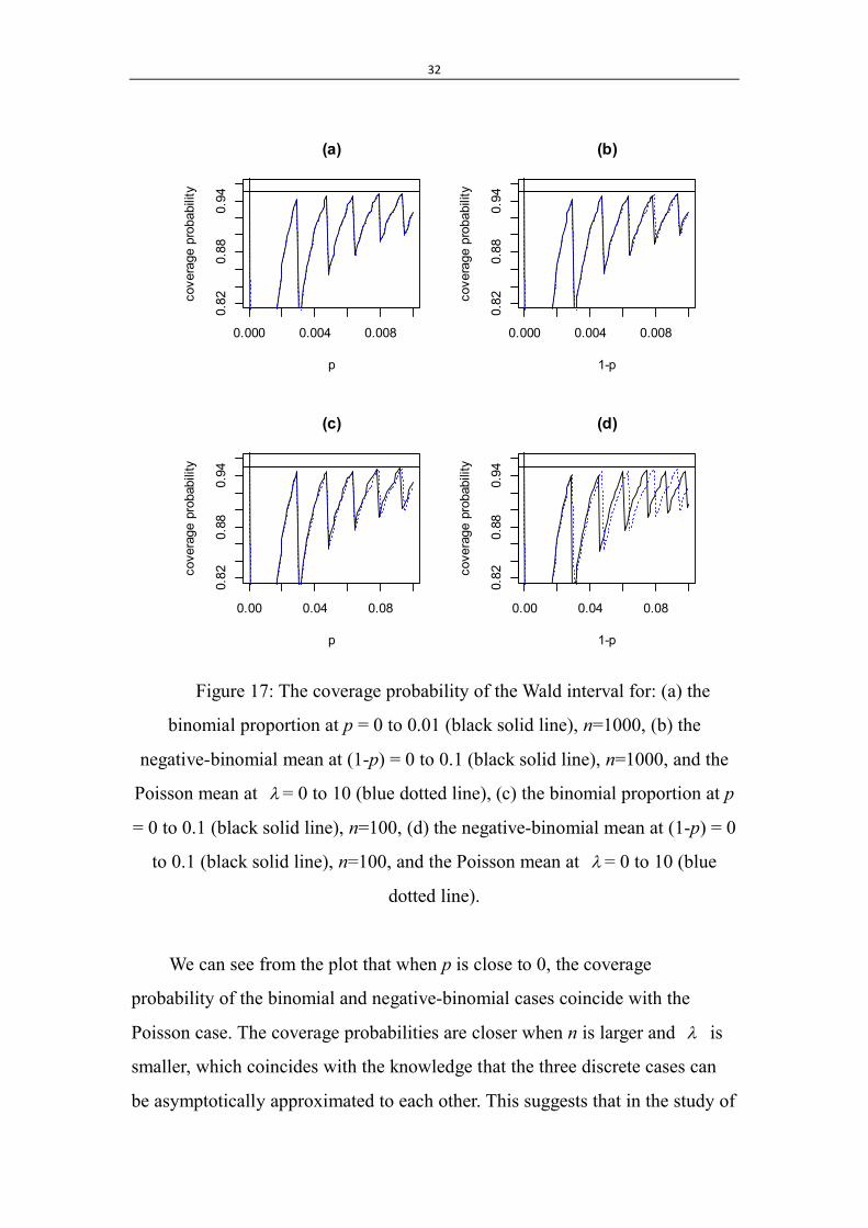
Figure 17: The coverage probability of the Wald interval for: (a) the

binomial proportion at p = 0 to 0.01 (black solid line), n=1000, (b) the

negative-binomial mean at (1-p) = 0 to 0.1 (black solid line), n=1000, and the

Poisson mean at = 0 to 10 (blue dotted line), (c) the binomial proportion at p

= 0 to 0.1 (black solid line), n=100, (d) the negative-binomial mean at (1-p) = 0

to 0.1 (black solid line), n=100, and the Poisson mean at = 0 to 10 (blue

dotted line).

We can see from the plot that when p is close to 0, the coverage

probability of the binomial and negative-binomial cases coincide with the

Poisson case. The coverage probabilities are closer when n is larger and is

smaller, which coincides with the knowledge that the three discrete cases can

be asymptotically approximated to each other. This suggests that in the study of

0.000 0.004 0.008

0.82

0.88

0.94

(a)

p

cove

rage

pro

babi

lity

0.000 0.004 0.008

0.82

0.88

0.94

(b)

1-p

cove

rage

pro

babi

lity

0.00 0.04 0.08

0.82

0.88

0.94

(c)

p

cove

rage

pro

babi

lity

0.00 0.04 0.08

0.82

0.88

0.94

(d)

1-p

cove

rage

pro

babi

lity

33

confidence intervals, when one of the three cases is hard to calculate, we can

use the asymptotical approximation to the other two.

7. Empirical examples

7.1 Female births proportion

To illustrate the differences between the confidence intervals, I will give a brief

example of the binomial case below. The data is the number of girls and boys

born in Paris from 1745 to 1770, and it is from Gelman (2004). It was first

studied by Laplace and was used to estimate the proportion of female births in

a population, to see if the female births in European populations was less than

0.5. A total of 241,945 girls and 251,527 boys were born in that period.

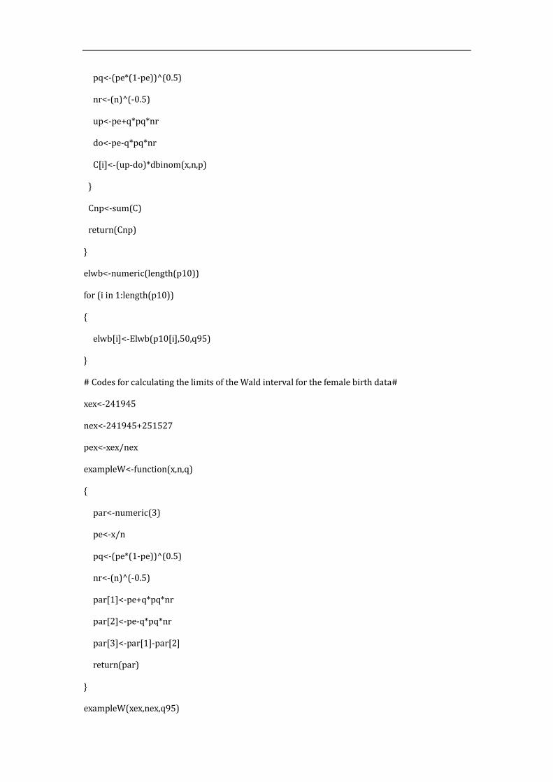
So in this example n=493,472 and the point estimation of the proportion is

ˆ 0.4902912Xpn

. I calculated the limits and length of the Wald interval and

the alternative confidence intervals for this binomial proportion, and the results

are in Table 1.

Table 1: 95% Confidence intervals for the female births proportion

Confidence Interval Lower limit Upper Limit Length

Wald 0.488896465 0.491686020 0.002789555

Wilson 0.488896546 0.491686090 0.002789544

Agresti-Coull 0.488896546 0.491686090 0.002789544

Clopper-Pearson 0.488895512 0.491687087 0.002791575

Likelihood ratio 0.488896538 0.491686050 0.002789512

Jeffreys 0.488896525 0.491686074 0.002789548

Bayesian HPD 0.488896525 0.491686074 0.002789548

We can see from the table that, the Agresti-Coull interval and Wilson score

interval get the same limits and length, Jeffreys interval and Bayesian HPD

34

interval also get the same results. The Clopper-Pearson interval is the longest,

and the likelihood-ratio interval is the shortest. Among these intervals, only the

Wald interval is symmetric. From this result we can also see that although the

Clopper-Pearson interval is the longest, if we focus on the aim that to see if the

female births was less than 0.5, it is better to choose the Clopper-Pearson interval to

suggest that at the 95% confidence level, 0.5 is beyond the upper bound of the

Clopper-Pearson interval. As the Clopper-Pearson interval is always

conservative, so even if 0.5 is above the upper limits of all these intervals, the

Clopper-Pearson interval can support the result best.

7.2 The horse kick data

Quine and Seneta (2006) introduced Bortkiewicz’s (1898) horse kick data set,

which describes the numbers on men killed by horse kicks in the Preussian

Army from 1875 to 1894, and Bortkiewicz showed in his book that this data

follows a Poisson distribution.

There are 280 observations from 14 corps in the army over 20 years, so

the variable ijX (i= 1,…, 20; j= 1,…,14) records the number of deaths by

horse kick in year 1874+i for corps j. Bortkiewicz showed in his book that

~ ( )ij jX Pois , and calculated the point estimator of j by ˆ20

iji

j

X

. I

calculated the limits and length of the Wald interval and the alternative

confidence intervals for these Poisson means, the results of corps G are in

Table 2, and the results of the rest of the 14 corps are in the appendix (Table

3~15).

We can see from these tables that, when n is small, the differences

between different intervals are larger than in the former example. The Wald

interval is of the shortest length, and the exact interval is of the longest. In this

example I would like to recommend the likelihood ratio interval for it is of

35

relatively shorter length, and the behavior of its coverage probability is less

chaotic than the Wald interval.

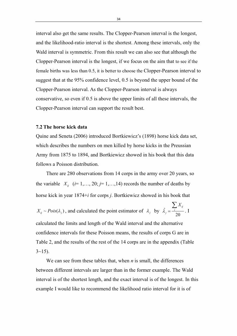
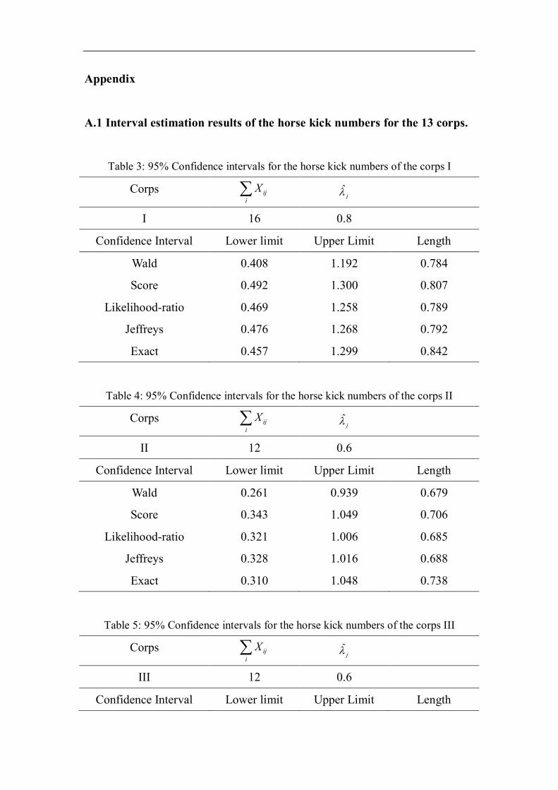
Table 2: 95% Confidence intervals for the horse kick numbers of the corps G

Corps iji

X ˆj

G 16 0.8


Wald 0.408 1.192 0.784

Score 0.492 1.300 0.807

Likelihood-ratio 0.469 1.258 0.789

Jeffreys 0.476 1.268 0.792

Exact 0.457 1.299 0.842

References

[1] Agresti, A. & Coull, B.A. 1998, "Approximate is Better than "Exact" for

Interval Estimation of Binomial Proportions", American Statistician, vol. 52,

no. 2, pp. 119-126.

[2] Barker, L. 2002, "A comparison of nine confidence intervals for a poisson

parameter when the expected number of events is ≤ 5", American Statistician,

vol. 56, no. 2, pp. 85-89.

[3] Bortkiewicz, L. von (1898). Das Gesetz der kleinen Zahlen: Teubner,

Leipzig

[4] Brown, L.D., Cai, T.T. & DasGupta, A. 2001, "Interval estimation for a

binomial proportion", Statistical Science, vol. 16, no. 2, pp. 101-133.

[5] Brown, L.D., Cai, T.T. & DasGupta, A. 2002, "Confidence intervals for a

binomial proportion and asymptotic expansions", Annals of Statistics, vol. 30,

no. 1, pp. 160-201.

[6] Brown, L.D., Cai, T.T. & DasGupta, A. 2003, "Interval estimation for

exponential families", Statisticl Sinica, vol. 13, pp. 19-49.

[7] Clopper, C. J. & Pearson, E. S. 1934, "The use of confidence or fiducial

limits illustrated in the case of the binomial", Biometrika, vol. 26, pp. 404-413.

[8] Fay P. M. & Feuer J. E. 1997, "Confidence intervals for directly

standardized rates: a method based on the gamma distribution", Statistics in

Medicine, vol. 16, pp.791-801.

[9] Gelman, A. (2004). Bayesian data analysis . 2. ed. Boca Raton: Chapman

& Hall

[10] Quine M. P. & Seneta E. 2006, "Bortkiewicz’s data and the law of small

numbers", International Statistical Institute, vol. 55, pp. 173-181.

[11] Rao, C. R. (1973). Linear statistical inference and its applications: Wiley,

New York.

[12] Severini T. A. 1991, "On the Relationship Between Bayesian and

Non-Bayesian Interval Estimates", Journal of the Royal Statistical Society.

Series B (Methodological), vol. 53, no. 3, pp. 611-618.

[13] Wang, W. 2006, "Smallest confidence intervals for one binomial

proportion", Journal of Statistical Planning and Inference, vol. 136, no. 12, pp.

4293-4306.

[14] Wilson, E. B. 1927, "Probable inference, the law of succession, and

statistical inference", J. Amer. Statist. Assoc., vol. 22, pp. 209-212.

Appendix

A.1 Interval estimation results of the horse kick numbers for the 13 corps.

Table 3: 95% Confidence intervals for the horse kick numbers of the corps I

Corps iji

X ˆj

I 16 0.8


Wald 0.408 1.192 0.784

Score 0.492 1.300 0.807


Jeffreys 0.476 1.268 0.792

Exact 0.457 1.299 0.842

Table 4: 95% Confidence intervals for the horse kick numbers of the corps II

Corps iji

X ˆj

II 12 0.6


Wald 0.261 0.939 0.679

Score 0.343 1.049 0.706


Jeffreys 0.328 1.016 0.688

Exact 0.310 1.048 0.738

Table 5: 95% Confidence intervals for the horse kick numbers of the corps III

Corps iji

X ˆj

III 12 0.6


Wald 0.261 0.939 0.679

Score 0.343 1.049 0.706


Jeffreys 0.328 1.016 0.688

Exact 0.310 1.048 0.738

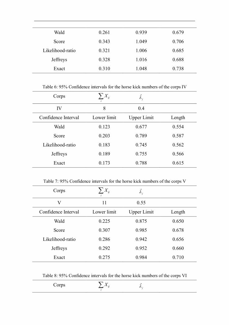
Table 6: 95% Confidence intervals for the horse kick numbers of the corps IV

Corps iji

X ˆj

IV 8 0.4


Wald 0.123 0.677 0.554

Score 0.203 0.789 0.587


Jeffreys 0.189 0.755 0.566

Exact 0.173 0.788 0.615

Table 7: 95% Confidence intervals for the horse kick numbers of the corps V

Corps iji

X ˆj

V 11 0.55


Wald 0.225 0.875 0.650

Score 0.307 0.985 0.678


Jeffreys 0.292 0.952 0.660

Exact 0.275 0.984 0.710

Table 8: 95% Confidence intervals for the horse kick numbers of the corps VI

Corps iji

X ˆj

VI 17 0.85


Wald 0.446 1.254 0.808

Score 0.531 1.361 0.831


Jeffreys 0.514 1.330 0.816

Exact 0.495 1.361 0.866

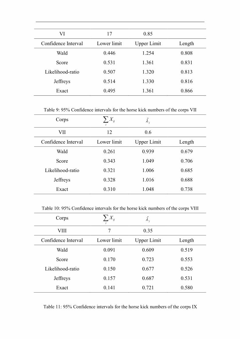
Table 9: 95% Confidence intervals for the horse kick numbers of the corps VII

Corps iji

X ˆj

VII 12 0.6


Wald 0.261 0.939 0.679

Score 0.343 1.049 0.706


Jeffreys 0.328 1.016 0.688

Exact 0.310 1.048 0.738

Table 10: 95% Confidence intervals for the horse kick numbers of the corps VIII

Corps iji

X ˆj

VIII 7 0.35


Wald 0.091 0.609 0.519

Score 0.170 0.723 0.553


Jeffreys 0.157 0.687 0.531

Exact 0.141 0.721 0.580

Table 11: 95% Confidence intervals for the horse kick numbers of the corps IX

Corps iji

X ˆj

IX 13 0.65


Wald 0.297 1.003 0.707

Score 0.380 1.112 0.732


Jeffreys 0.364 1.080 0.716

Exact 0.346 1.112 0.765

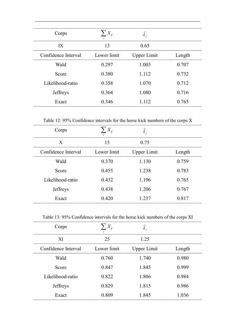
Table 12: 95% Confidence intervals for the horse kick numbers of the corps X

Corps iji

X ˆj

X 15 0.75


Wald 0.370 1.130 0.759

Score 0.455 1.238 0.783


Jeffreys 0.438 1.206 0.767

Exact 0.420 1.237 0.817

Table 13: 95% Confidence intervals for the horse kick numbers of the corps XI

Corps iji

X ˆj

XI 25 1.25


Wald 0.760 1.740 0.980

Score 0.847 1.845 0.999


Jeffreys 0.829 1.815 0.986

Exact 0.809 1.845 1.036

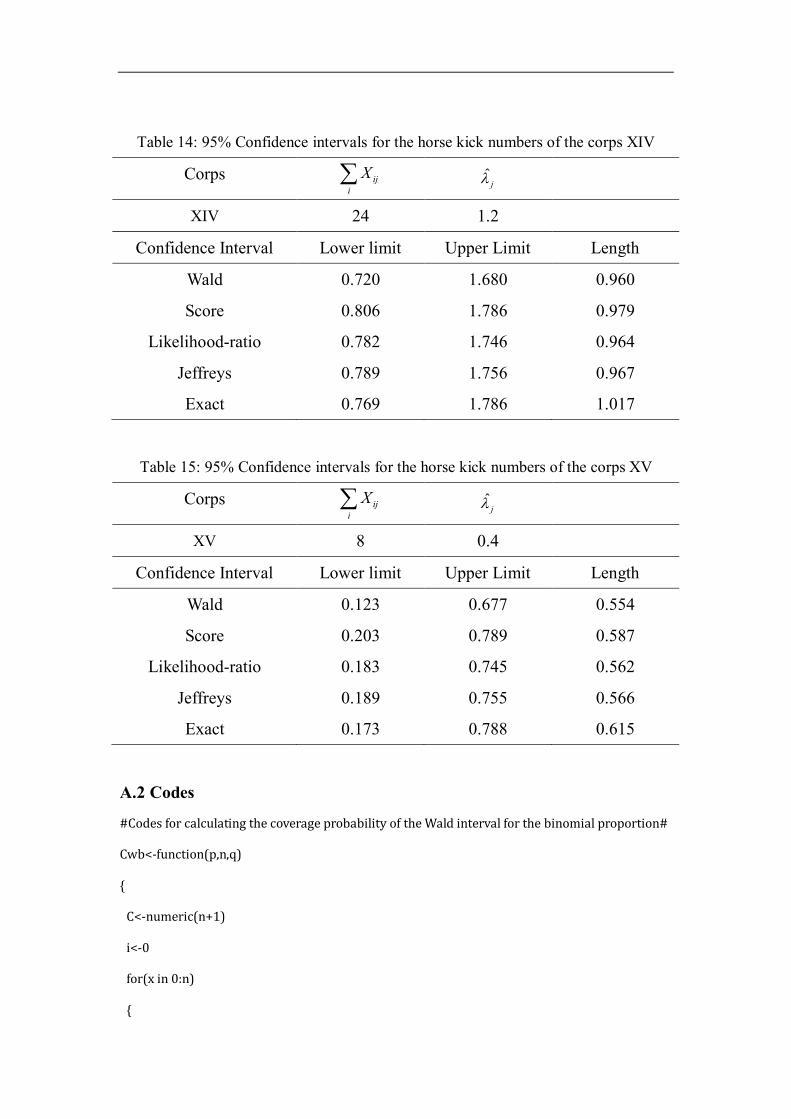
Table 14: 95% Confidence intervals for the horse kick numbers of the corps XIV

Corps iji

X ˆj

XIV 24 1.2


Wald 0.720 1.680 0.960

Score 0.806 1.786 0.979


Jeffreys 0.789 1.756 0.967

Exact 0.769 1.786 1.017

Table 15: 95% Confidence intervals for the horse kick numbers of the corps XV

Corps iji

X ˆj

XV 8 0.4


Wald 0.123 0.677 0.554

Score 0.203 0.789 0.587


Jeffreys 0.189 0.755 0.566

Exact 0.173 0.788 0.615

A.2 Codes

#Codes for calculating the coverage probability of the Wald interval for the binomial proportion#

Cwb<-function(p,n,q)

{

C<-numeric(n+1)

i<-0

for(x in 0:n)

{

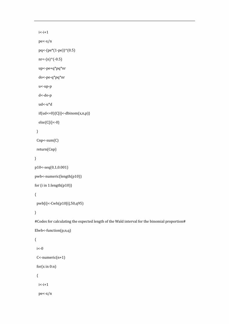
i<-i+1

pe<-x/n

pq<-(pe*(1-pe))^(0.5)

nr<-(n)^(-0.5)

up<-pe+q*pq*nr

do<-pe-q*pq*nr

u<-up-p

d<-do-p

ud<-u*d

if(ud<=0){C[i]<-dbinom(x,n,p)}

else{C[i]<-0}

}

Cnp<-sum(C)

return(Cnp)

}

p10<-seq(0,1,0.001)

pwb<-numeric(length(p10))

for (i in 1:length(p10))

{

pwb[i]<-Cwb(p10[i],50,q95)

}

#Codes for calculating the expected length of the Wald interval for the binomial proportion#

Elwb<-function(p,n,q)

{

i<-0

C<-numeric(n+1)

for(x in 0:n)

{

i<-i+1

pe<-x/n

pq<-(pe*(1-pe))^(0.5)

nr<-(n)^(-0.5)

up<-pe+q*pq*nr

do<-pe-q*pq*nr

C[i]<-(up-do)*dbinom(x,n,p)

}

Cnp<-sum(C)

return(Cnp)

}

elwb<-numeric(length(p10))

for (i in 1:length(p10))

{

elwb[i]<-Elwb(p10[i],50,q95)

}

# Codes for calculating the limits of the Wald interval for the female birth data#

xex<-241945

nex<-241945+251527

pex<-xex/nex

exampleW<-function(x,n,q)

{

par<-numeric(3)

pe<-x/n

pq<-(pe*(1-pe))^(0.5)

nr<-(n)^(-0.5)

par[1]<-pe+q*pq*nr

par[2]<-pe-q*pq*nr

par[3]<-par[1]-par[2]

return(par)

}

exampleW(xex,nex,q95)