


Languages
Pages
Legal

Page 1
Interdependent Voting in
Two-Candidate Voting Games
Abstract
The election of a political candidate is a public good for all those who prefer it and a
public bad for those who are opposed. Given free-rider problems and other features of collective
action, the probability that any one voter will vote for a preferred candidate is unlikely to be
independent of the voting probabilities of all others with the same electoral preference, as is so
often assumed. Interdependent voting probabilities are, therefore, likely to be the norm rather
than the exception. We make no assumption about this interdependence other than a generalized
concavity condition.
The point of departure for this paper is independent voting in the context of a two-
candidate, regular concave voting game. Such games always have a unique, asymptotically
stable equilibrium platform. This platform is not the ideal point of the median voter, however. It
is also, in general, not Pareto optimal. With interdependent voting, the unique equilibrium is
preserved when candidates have the same initial endowments. If one candidate is advantaged (so
the game is not symmetrical), however, plurality-maximizing candidates will cycle endlessly.
A candidate advantage creates a convex set of platform choices, none of which can be
defeated by the disadvantaged opponent. An equilibrium without convergence is achieved if we
assume that the advantaged candidate chooses from an undefeatable set a platform that
Page 2
maximizes utility while an opponent maximizes her plurality. The set of undefeatable platforms
collapses on a unique winning platform as the advantage disappears.
Key Words: Voting games, vote production, electoral competition.
JEL Classification: H00, H10, H11

Page 3
Interdependent Voting in
Two-Candidate Voting Games
by
John C. Goodman
and
Philip K. Porter
How do voters interact in support of the election of candidates they prefer? This is a
neglected topic in public choice economics and the oversight turns out to be of considerable
importance.1 Interdependent voting can wreak havoc in voting games that otherwise have unique
and stable equilibriums. With even the simplest interaction, candidate plurality functions can
have multiple peaks and plurality-maximizing politicians can get caught up in endless cycles.
In the modern era, interest in voting theory was sparked when Arrow (1963) drew
attention to the paradox of voting, a condition under which no alternative can win a majority vote
over all others.2 For a while, it was unclear whether the paradox was a curiosity or something to
be routinely expected. With single-peaked preferences in one dimension, voters’ ideal points can
be arrayed on a line along which the median voter’s preference dominates all alternatives
(Hotelling 1929; Downs 1957; Black 1958; Enelow and Hinich 1984). However, about two
decades ago it became clear that in multiple dimensions instability is the rule, not the exception,
1 There have been a number of models of campaign contributions, including Ben-Zion and Eytan (1974), Welch
(1984) Bental and Ben-Zion (1975) and Welch (1980). None of these, however, investigated the impact of
campaign contributions on the existence and stability of voting equilibrium. Also see Cook, et. al.(1974), and
Sankoff and Mellos (1972).
2 The phenomenon had been discovered almost two hundred years earlier by Condorcet (1785) and one hundred
years later by Dodgson (1876). For a discussion of these and other early contributions see Black (1958), Riker
(1961), and Mueller (2003)

Page 4
and that voting cycles will typically range all over the issue space (Ordeshook and Shepsle,
1982).3
These conclusions, however, were based on one-person-one-vote models in which voting
outcomes are dependent on preferences alone. Because there is nothing voters can do to increase
or decrease their level of support for a favored candidate, these models lacked the concept of
marginalism, which so imbues the rest of economic theory.4 One way to incorporate the
marginalist principle is to allow voter abstention and to assign to each voter a probability of
voting which varies, depending on the voter’s interest in the outcome. Hinich, Ledyard and
Ordeshook, (1972) showed that this modification is sufficient to generate a unique equilibrium at
which competing candidates converge to the same platform under reasonable assumptions.5
The introduction of marginalism into voting theory was short-lived, however. Over the
past 25 years or so a new literature has emerged on probabilistic voting.6 Today, probabilistic
voting usually means that candidates do not know exactly how voters will vote. The
probabilities, therefore, are properties of the state of knowledge of candidates, rather than
characteristics of voters themselves (Coughlin, 1991). Under assumptions similar to those we
incorporate herein, conventional probabilistic voting models have unique, stable equilibriums.
But they pay two heavy prices for this result. First, the models break down for small voting
3 A particularly depressing judgment was rendered by Riker, who concluded that politics, not economics, “is the
dismal science because we have learned from it that there are no fundamental equilibria to predict.” (1982, p. 19).
4 The principle of marginalism in this context holds that participants in the political system can always incrementally
increase or decrease the level of effort they are willing to make to affect the political outcome, and these incremental
changes always have an impact on political equilibrium, no matter how small (Goodman, 1976).
5 They justified their assumptions about voter behavior based on the alienation and indifference hypotheses (see
Hinich, Ledyard and Ordeshook 1972, and Davis, Hinich and Ordeshook 1970). For other formulations of this
approach, see Hinich, Ledyard and Ordeshook (1973), McKlvey (1975), Hinich (1977) and Ledyard (1984).
6 See, e.g., Enelow and Hinich, 1981, 1984; Ordeshook, 1971; Coughlin, 1982, 1986, 1991; Coughlin and Nitzan,
1981a, 1981b; Coughlin, Mueller, and Murrell, 1990; Feldman and Lee, 1988; and the surveys in Mueller, 2003 at p.
263; and in Lafay, 1993.

Page 5
groups where the uncertainty assumption collapses. Second, they relegate the voter to a
completely passive role. The voter’s only function is to have preferences (Coughlin, 1990).
The single, most important feature of all democracies is that elections are collective
consumption goods. Every candidate’s election is a public good for all those who favor it and a
public bad for those who are opposed. As a result, people have an incentive not to vote, relying
on others of similar interest to make the effort to elect a preferred candidate (Downs, 1957).
Among the group of supporters, this form of free-riding can be overcome to some degree by peer
pressure in the form of persuasion, personal appeals, participation in get-out-the-vote efforts, and
other overt actions to influence electoral outcomes (Olson, 1965). To the extent that people act
in this way, and are successful, any one voter’s behavior will not be independent of the behavior
of all others.
Accordingly, we introduce the concept of a vote production function to link the efforts of
citizens to the vote totals they produce for the candidates they prefer. Note: our interest here is
not in how voters interact with each other, but that they interact. We make no assumption about
the interaction other than a generalized concavity condition.7
In Section I we model electoral competition as a two-person concave voting game. In
Section II we consider the special case of a linear vote production function (independent voting),
and show that every regular concave voting game has a unique, asymptotically stable equilibrium
at which both candidates converge to the same platform. We show that the same equilibrium
7 The observation that votes depend on more than voter preferences - for example, candidate popularity or perceived
trustworthiness (Ansolabehere and Snyder, 2000; Groseclose, 2001; Schofield, 2003 & 2004), campaign advertising
(Ashworth, 2006; Prat, 2002, Ansolabehere and Iyengar, 1996; Gerber, 1998) and party affiliation (Adams, 1998) –
implies that votes are generated by a process that combines the inputs of platform promises, money, political
association, and valence among other things. For our purposes in this paper we assume the various inputs can be
summarized by a single numeraire input we call supporter or voter “effort.” The law of diminishing marginal
returns motivates the assumption that the production of votes is concave over effort.

Page 6
persists even if there is asymmetry that gives a natural advantage to one of the two candidates.
Further, if the candidates are constrained to take different positions on some issues, they will
converge in all issue dimensions where they are not constrained.
In Section III we evaluate the welfare consequences of the equilibrium points for regular
concave voting games. Against the heartening discovery that the political process has a
determinate outcome is the disheartening discovery that the outcome will almost never be Pareto
optimal. This conclusion is similar to the results we found for the regulation of output and price,
the production of public goods and government supply of other goods and services (Goodman
and Porter 1985, 1988 and 2004).
In Section IV, we show that in the face of nonlinear vote production functions
(interdependent voting) candidate plurality functions can have multiple peaks and vote cycling
can occur. Nonetheless, such games can have a unique equilibrium at which the two candidates
may converge. When asymmetry is introduced, however, the voting game will not have an
equilibrium for plurality-maximizing candidates, but will instead lead to endless cycles. This
finding strongly suggests that instability in democratic voting is more likely to arise from the
way in which voter preferences are translated into votes than from the distribution of the
preferences themselves.8
These results cause us to question three conventional assumptions about voting games:
(1) that candidates maximize pluralities, (2) that a Nash equilibrium is the appropriate
equilibrium concept and (3) that candidates engage in conventional platform adjustments when
they are not in equilibrium. In Section V, we set aside all three assumptions and demonstrate
8 Non-convergence in stochastic models of voting can be introduced by voter uncertainty (Berger, Munger and
Pothoff, 2000). Convergence away from the electoral center is predicted in models with an advantaged candidate
(Ansolabehere and Snyder, 2000; Groseclose, 2001; Schofield, 2003).

Page 7
that an advantaged candidate has access to a set of points that cannot be defeated by an
opponent.9 Moreover, this set is a convex set that converges to the unique winning platform
described in Section IV as the advantage disappears.
In Section VI we consider what a candidate might do with an advantage. Maximizing
utility over the set of undefeatable platforms always produces a unique platform choice.
However, if the disadvantaged candidate maximizes her plurality, the candidates’ platforms will
differ.
In the long run, candidate advantages are likely to disappear, making the competition
symmetrical.10
In this case, democratic voting is likely to produce a unique winning platform
that is independent of the preferences of the candidates themselves. Significantly, this unique
winning platform is not necessarily the ideal point for the median voter. It is instead a platform
that equates the “marginal political prices” groups of voters on either side of each issue are
willing to pay to obtain a dollar’s worth of benefit from the political system. This result is
consistent with our own previous work as well as the work of Becker (1983) and Peltzman
(1984).
I. The Voting Game
We model the political system as a two-person, zero sum, symmetric, non-cooperative
game. Candidate 1 and candidate 2, denoted by superscripts 1 or 2, adopt the platforms
1 1 1 1
1 2( , , , )nX x x x and 2 2 2 2
1 2( , , , )nX x x x , respectively. Each platform issue, ix , is chosen
from issue space , an n-dimensional compact, convex set. We assume that for each voter, j,
9 Feld and Gorfman (1991) demonstrate this for advantaged candidates who enjoy voter loyalty.
10 In two party competitions one party might possess an advantage in any given election that derives from a
candidate’s seniority, wealth, or name recognition but in the long run these advantages disappear.

Page 8
there is a benefit function 1 2( , , , )j
nx x x which is a positive, concave function, with ,xx the
Hessian of second-order derivatives of j , negative definite.11
Our benefit functions are fully
analogous to voter utility functions, commonly used in voting models. The difference is one of
interpretation. The standard approach is to assume that voters derive utility from political
platforms. By contrast, we assume that voters derive utility from states of the world created by
those platforms. This allows us to make the kind of welfare judgments familiar to economists in
other contexts.12
We denote by 1 2( , )jL X X the support voter j will give to a candidate with platform 1X ,
given an opponent who endorses platform 2.X Similarly, 2 1( , )jL X X is the support voter j will
give to a candidate with platform 2 ,X given an opponent who endorses 1.X We assume
throughout that L is a uniform measure of support, regardless of the preferred candidate, and that
voters always support the candidate whose platform they prefer. Thus:
(2a)
1 2 1 2
1 2
[ ( ), ( )] ( ) ( )
( , )
0 .
j j j j j
j
l X X if X X
L X X
otherwise
(2b)
2 1 2 1
2 1
[ ( ), ( )] ( ) ( )
( , )
0 .
j j j j j
j
l X X if X X
L X X
otherwise
We assume that the function jL is continuous and the function jl is continuous and twice
differentiable with
11
For the proof of the following theorems, it is not necessary for every benefit function to be concave. However,
they must be strictly concave on the average.
12 Imagine the platform issues are regulated product prices. We do not assume that voters get utility from the prices.
Instead, the prices give rise to consumer and producer surplus. Further, the optimal vector of prices is the one that
maximizes the total surplus (See Goodman and Porter 1988).

Page 9
(3) 1 2 11 220, 0, 0, 0.j j j jl l l l
(4) 1 2 2 1
1 2lim limj jl l
We model the support that voters give to candidates rather than the votes they give for
several reasons. First, in a world of campaign finance, the potential influence a voter can have
on an election extends well beyond the mere act of voting. Second, unlike probabilistic votes,
support is not constrained to the closed interval [0, 1] and, therefore, not subject to the
impossibility result identified by Kirchgassner (2000). Finally, the fact that votes are produced
by combining the support of individuals, rather than simply summing over individual
preferences, is the insight that motivates the findings of this paper.
If voters act independently of each other, the sum of support is analogous to the sum of
the voting probabilities and our model yields the same results as the probabilistic voting model.13
However, when voters interact their efforts are inputs into a process that creates votes for the
candidate they prefer. Further, the electoral value of a voter’s effort on behalf of one candidate
(given the candidate’s coalition of supporters) may not equal the electoral value of that same
effort when dedicated to another candidate (given the second candidate’s coalition of
supporters).
We denote by the function V(L) the transformation of support by voters into actual votes
for the candidates whose platforms they prefer and offer the following:
Definition: A vote production function identifies a candidate’s unique vote total, given
the cumulative support of all voters who prefer the candidate’s election to that of an opponent.
13
Note that the measures of support jL can be mapped onto the interval [0, 1] and preserve the cardinal properties
of support by simply dividing each individual’s support by the maximum individual support offered.

Page 10
Although we call this function a vote production function, it differs from its counterpart
in standard production theory. Unlike an entrepreneur or a firm, candidates do not control all of
the ways in which inputs combine to produce an output. In fact, in the model used here
candidates have only one function: to select platforms. By contrast, voters themselves “produce”
votes through their actions and interactions with each other.
The way in which preferences are translated into votes is undoubtedly complex. The
election of a candidate is a public good for all the supporters and a public bad for all the
opponents and, therefore, suffers from expected free-rider problems. Also, the composition of
the groups of voters who favor or oppose a candidate will tend to change whenever a platform
changes. It is not our goal here to explore these complexities. Rather in what follows we show
that anything more complicated than a linear relationship is likely to produce endless cycling.
Each candidate is assumed to maximize an expected plurality (the difference between the
candidate’s own votes and the votes for the opponent) given by:
(5a) 1 1 2 1 2 2 1, ( , ) ( , )j j
j j
X X V L X X V L X X
(5b) 2 2 1 2 1 1 2, ( , ) ( , )j j
j j
X X V L X X V L X X
The game will be said to have a Nash equilibrium if neither candidate can improve her
position by any unilateral move. That is, 1* 2*( , )X X is an equilibrium if:
(6a) 1 1* 2* 1 1 2* 1( , ) ( , )X X X X X
(6b) 2 2* 1* 2 2 1* 2( , ) ( , )X X X X X

Page 11
At a point other than equilibrium we assume the two candidates continuously adjust their
platforms at constant rates, such that:
(7a) 0,,1// 11111 rnixrdtdx ii
(7b) 0,,1// 22222 rnixrdtdx ii
We consider other adjustment assumptions below.
II. Independent Voting
For the case of a linear vote production function, (with independent voter behavior), we
have:
(8) ( ) ,i iV L L where 1 1 2( , )j
j
L L X X and 2 2 1( , ).j
j
L L X X
In other words, a candidate’s vote total is given by summing the support of all who favor his or
her election.
Definition: Any game described by conditions (1) through (8) is a regular concave voting
game.
Following the lead of Hinich, Ledyard and Ordeshook (1972), we offer two theorems and
three corollaries.
Theorem I: For every regular concave voting game, (a) there is a unique equilibrium
1* 2*( , )X X and (b) from any initial point in the issue space, say 2
0
1
0 , XX , a solution to equation
set (7), tXtX 21 , , exists and converges to *2*1 , XX , i.e. *11lim XtXt and
*22lim XtXt .

Page 12
Proof: Goodman’s theorem (1980) states that every game possesses a unique and
asymptotically stable equilibrium provided that each player’s payoff (plurality) function is
strictly concave in his own strategy (Hessian is negative definite) and convex in the strategies of
all the opponents (sum of the Hessians is positive semi-definite) and the sum of all payoff
functions is concave.14
From the fact that xx is negative definite, it follows that 1 1X X is
negative definite and 2 2X X is positive definite for candidate 1, and 2 2X X
is negative definite
and 1 1X X is positive definite for candidate 2. Since the sum of the payoff functions is always
zero, the conditions of Goodman’s theorem are met. Q.E.D.
Theorem II: The equilibrium 1* 2*( , )X X is a point at which the two candidates converge
in every issue dimension, i.e., 1* 2* *
i i ix x x for all i.
Proof: Note that from the requirement of symmetry, if 1* 2*( , )X X is an equilibrium,
2* 1*( , )X X , 1* 1*( , )X X and 2* 2*( , )X X must also be equilibriums. But since the equilibrium is
unique, we must have 1* 2*X X . In equilibrium, both candidates endorse the same platform and
1* 2* *X X X .
How important is symmetry? One way to violate the symmetry condition is to give one
candidate an initial endowment of resources (core support), 0L , that is not available to the other
candidate. Another way is to assume that because of biased voting, one candidate is the recipient
14
Goodman’s Theorem is a special case of a set of theorems proved by Rosen (1965). The assumptions of
concave/convex payoff functions are reasonable for a broad class of voting games. But they are not defensible for
every game. Coughlin (1986) and Feldman and Lee (1988) have shown that the required restrictions are
unreasonable in the context of unconstrained redistribution of income and Kirchgassner (2000) has shown that they
may break down in other cases. Ball (1999) has shown that they are also unreasonable if candidates have goals
other than vote maximization or plurality maximization.

Page 13
of more support than an opponent, even if the two platforms are identical. A third way is to
place constraints on the platforms of the two candidates.
Corollary I: If one candidate has initial resources, 0L , not available to the opponent, the
equilibrium point * *( , )X X will be unaffected.
Corollary II: If 21 LL when ,21 XX the equilibrium point * *,X X will be
unaffected.
Corollary III: If the two candidates are constrained on issue p so that 1 2
p px x then in
equilibrium 1 2 *
i i ix x x for all .i p
Theorem II says there is one platform that can defeat all others in a majority vote. The
three corollaries say that even with asymmetry two candidates will always converge at the
winning platform unless they are explicitly constrained from doing so.
Proof: Note that in introducing non-symmetry we have not altered any of the conditions
required for the proof of Theorem I. So we can continue to be assured of a unique equilibrium.
Consider any platforms, A and B, defined over the m-dimensional space nm that delineates
the choices of candidates on issues where they are not constrained. Let 1( , )A A a and
2( , )A A a when the candidates do converge and assume there is an equilibrium (B, A),
B ≠ A, where they do not. Then we must have 1 2( , ) ( , )B A A B a . Otherwise one of the
two candidates could improve his or her plurality by simply matching the opponent’s position.
Hence 1 1( , ) ( , )B A A A a . But from the strict concavity of 1 we must have
Page 14
1 11 , , ,A A A for ,10 contradicting the assumption that the point (B,
A) is an equilibrium.15
Q.E.D.
In what follows, we assume symmetry unless otherwise indicated.
III. Welfare Consequences
For an interior solution, the first order conditions for a maximum for each candidate
require:
(9) 1 2 0j j
j j
k kj ji i
l lx x
1, ,i n and 1, 2k
at the equilibrium point *.X Note that 1
jl is the marginal support voter j is willing to give a
favored candidate for an extra dollar’s worth of benefit from the political system. Thus condition
(9) says that the cumulative support per dollar of expected benefit for those who favor an
increase in ix must be equal to the support per dollar of expected benefit for all those opposed.
At the equilibrium platform, “political prices” offered by opposing groups of voters must be
equal.
Note that the equilibrium platform does not necessarily represent the preferences of the
median voter and in the general case will almost never do so. In fact, unlike the median voter
result in one-man-one-vote deterministic models, the equilibrium platform described here is
influenced by the preferences of every voter and his willingness to act. Also, any change in the
15
1 is strictly concave in any subset of the issues. To see this, array the issues so that those in the subset come
first in 1 1
.X X Because the principle minors of 1 1X X alternate in sign beginning with 1 0,M the sufficient
condition for strict concavity in the subset of issues is met.

Page 15
preferences or the marginal support of any voter will change the equilibrium, reflecting the
marginalist principle.
What are the expected welfare consequences of the equilibrium points in concave voting
games?
Theorem III: The platform 1* 2*( , )X X is Pareto optimal if 1 2
j jl l for all voters.
Proof: Note that if 1 2
j j jl l for every voter, then condition (9) reduces to the first
order condition for maximizing 1 2( , , , ),j
nj
x x x the sum of the benefit functions for all
voters. A similar argument applies to constrained solutions. Q.E.D.
According to Theorem III, optimality is ensured if the marginal effort is the same for all
voters. But since there is no mechanism that induces such equality, we are left with the
pessimistic conclusion that optimality will almost never occur. Plurality maximizing candidates
will always make Pareto adjustments if they can compensate the losers for their losses. But such
compensation will generally require individualized tax rates and/or benefit payments. And since
no extant political system has such individualized programs, optimality is not an expected
outcome, at least in large-scale majority voting systems.16
IV. Interdependent Voting
We now consider a nonlinear function )(LV with interdependent voter behavior, where
16
It is common practice to regard majority voting equilibrium as Pareto optimal, since if it were possible to make
one voter better off without making some other voter worse off one of the candidates would surely do so. As shown
in Goodman and Porter (1985), this observation is true but trivial. Global optimality occurs only if the choice set
open to politicians is the same as the choice set theoretically available to society as a whole. But this assumption is
unwarranted. In conventional economics, non-optimal results occur because economic actors find that they are
unable to compensate the losers for their losses. The same thing happens in politics. On other examples of equating
electoral equilibrium with a social welfare optimum, see Coughlin (1982), Coughlin and Nitzan (1981a), Lindbeck
and Weibull (1987), and Mueller (2003 at p. 253).

Page 16
(10) 0LV
(11) 0.LLV 17
In general, nonlinerity means the plurality functions will not be differentiable at the
points where 1 2.i ix x The reason: when the candidates have not converged on issues other than
i, they will tend to have different quantities of the input L. Thus, the marginal product of a
contribution will be different, depending on whether the point 1 2
i ix x is approached from the left
or the right. Additionally, the plurality functions will not be everywhere concave. They may
have multiple peaks and valleys and they may not be stable. Nonetheless, a unique equilibrium
will still exist, provided that the candidates have the same initial endowment.
Theorem IV: With nonlinear vote production described by equations (10) and (11), and
,2
0
1
0 LL the platform *X is a unique equilibrium for the game.
Proof: Theorem 1 implies that 1 * 2 *( , ) ( , )L X X L X X for all *.X X Since V is
monotonic in L, 1 2( ) ( )V L V L whenever L1 > L
2. It follows that the platform X
* can defeat any
other platform in a majority vote. Hence, * *( , )X X must be an equilibrium for the game. Q.E.D.
Non-linearity by itself affects neither the winning platform nor the welfare properties of
that platform. The plurality function for candidate 1 is:
(12) 1 1 2 2 1
0 0(( , )) ( , ) .j j
j j
V L L X X V L L X X
17
One way an individual can give more support than a single vote is by providing information and applying peer
pressure that increases the vote support of others. As in conventional production theory we assume diminishing
marginal returns to support. If there are increasing marginal returns, the following conclusions still hold but the role
of leader and follower when there is a dominant candidate will be reversed.

Page 17
When *21 XXX both plurality functions are continuously differentiable. Hence,
the derivatives of 1 at * *( , )X X exist and the first-order necessary conditions for the
maximization of (12) that define an interior solution at * *( , )X X are:
(13) 1 2( ) ( ) 0 1, , .j j
j j
j ji i
dV dVl l i n
dL x dL x
Since 0L is the same for both candidates, equation (13) is equivalent to equation (9).
Let us again introduce asymmetry by positing a difference in initial endowments. Then
we have:
Theorem V: For V(L) nonlinear, 1 2
0 0 ,L L there exists no equilibrium for the game.
Proof: Without loss of generality assume candidate 1 has the larger initial endowment,
,2
0
1
0 LL and consider points where the candidates have the same platform. For a marginal
increase in platform plank ix candidate 2 will receive a differential contribution dL and her
opponent will receive .dL From condition (4) we know that if candidate 2 instead chooses a
marginal decrease in ix she will receive dL and her opponent will receive .dL Either
dL dL or .dL dL If the former, 2 2 1
0 0( ) ( ) 0L Ld V L dL V L dL . Since candidate 2,
with a smaller endowment, has a higher marginal product at a point of convergence [i.e., 1 2
0 0L L
implies that 1 2
0 0( ) ( )],L LV L V L candidate 2 can increase her plurality by choosing a higher value
of ix . If the latter case, 2 2 1
0 0( ) ( ) 0L Ld V L dL V L dL and candidate 2 can gain from a
marginal decrease in ix . Hence, no point of convergence can be an equilibrium.

Page 18
Let c be candidate 1’s plurality at any point of convergence, and consider a possible
equilibrium at 21 XX where the candidates do not converge. Then we must have
1 1 2 2 2 1, , .X X X X c Otherwise, one of the two candidates could increase her
plurality by simply matching the platform of the opponent. Thus the move 1 2 1 1, ,X X X X
maintains candidate 2’s plurality and from 1 1,X X we know she can increase her plurality by a
subsequent move. Hence, no divergent point 21, XX can be an equilibrium for the game.
Q.E.D.18
An example of candidate 2’s incentives is depicted in Figure I, where there is a single
issue and voters are grouped around two ideal points. Beginning at a point of convergence
Candidate 2 can gain by a movement in either direction. Note that the adjustment equations (7)
do not guarantee that she will move in the direction that maximizes her plurality, however.
Assume that both candidates always choose a plurality-maximizing platform, given a choice by
the opponent. The resulting cycling is depicted in Figure II, where the cycles function like an
oscillating super nova. Beginning at *x we experience wide swings which expand, contract and
expand again.19
Three properties of this example are interesting, especially if they hold for more complex
cases. First, with concave vote productions a challenger always improves her plurality by
moving away from the dominant candidate. Second, the dominant candidate improves his
18
Aragones and Palfrey (2002, 2004) demonstrate this for two candidate competition over a single issue. The
advantaged candidate has the incentive to copy the disadvantaged candidate while the latter has the incentive to
move away from the former. 19
Figures I and II are the result of a stylized example. The voter benefits, voter contributions, endowments, and the
vote production function together with a narrative are detailed in the appendix.
Page 19
plurality by chasing the challenger. Third, the pursuit of a Nash equilibrium requires substantial
flip flopping on the issues, as the cycles range over wide portions of the issue space.
V. Electoral Dominance
Some voters may penalize a candidate who flip-flops, just on principle. So, we are
interested in alternatives to myopic plurality maximization. If one candidate must pick a
platform and stick with it, regardless of the actions of an opponent, what platform should she
pick? Since in asymmetric voting games, one candidate will tend to have a natural advantage
over an opponent, we introduce the following:
Definition: Candidate 1 is a dominant candidate if there exists any platform X, *XX ,
such that 1 2 2, 0, .X X X
Importantly, dominance expands the range of options for the favored candidate since a
dominant candidate can adopt platforms other than *X and not be defeated. Let
(14) 2 2 2( ) : ( , ) ( , ) 0,X X V X X V X X X
be the set of platforms for dominant candidate 1 that cannot be defeated. Then
Theorem VI. (a) ( )X is a closed convex set defined by the endowments, 1
0L and 2
0 ,L (b)
1 2 1 2
0 0 1 0( : , ) ( : , )X L L X L L if 1 1
0 1L L , and (c) *( )X X as 1 2
0 0.L L
Proof: (a) Assume ( )X is not convex. This implies that there exists at least two
platforms for candidate 1, say X̂ and ,X in ( )X and some 2
0X and some 0 1 such that
1 2
0, 0X X and 1 2
0, 0,X X but ' 2
0, 0X X where .~
1ˆ' XXX Now
consider the advantage of candidate 1, given 2
0 .X From Theorem I, the differential support

Page 20
2 2
0 0[ ( , ) ( , )]j j
j
L X X L X X is a concave function of X. Hence, the greater-than-or-equal-to set
2 1 2 1 2 2 2 2 1
0 0 0 0 0 0 0( : , , ) : ( , ) ( , )H X X L L X L X X L X X L L is a convex set, containing all
platform choices for candidate 1, given ,2
0X for which her support plus her endowment are
greater than or equal to candidate 2’s support plus his endowment. Points in H are candidate 1
platforms that cannot be defeated by .2
0X Since X̂ and X must be in H, by its convexity so
must ,'X contradicting the assumption that 2
0X can defeat .X Including equal vote production,
closes the set.
(b) 2 1 2 2 1 2
0 0 0 0 1 0( : , , ) ( : , , )H X X L L H X X L L for every value of 2
0X when 1 1
0 1.L L
Therefore, 1 2 1 2
0 0 1 0( , , ) ( , , ).X L L X L L
(c) From (b) we know that ( )X shrinks as 1 2
0 0L L and by Theorem IV we know that
when the endowments are equal the only platform that cannot be defeated is X*. Q.E.D.
The boundary of ( )X is 1 2* 2 2* 2 1
0 0: ( , ) ( , )X L X X L X X L L , where 2*X is the
plurality-maximizing platform for candidate 2 given the platform of candidate 1. Boundary
points can result in electoral ties. Candidates who wish to assure election will choose to be on
the interior of ( )X . We therefore define the set
2 2 2( : ) : ( , ) ( , ) , .X X V X X V X X X By the logic employed in the proof of
Theorem VI, ( : )X is also a closed, convex set. Positive values of yield a set of points that
assure the election of the dominant candidate by a plurality greater than or equal to .20
When
there is uncertainty, being near the boundary of ( )X is risky since candidates may misperceive
20
The set ( : )X shrinks as increases. For high values of , ( : )X is empty.

Page 21
the scope of their advantage. Additionally, there are often unforeseen surprises in elections that
can reduce a candidate’s advantage. Uncertainty and an aversion to risk will make the dominant
candidate retreat to the interior of ( )X . A dominant candidate does not maximize his plurality
by choosing *X . But given any uncertainty about 1
0L and 2
0L the platform *X assures his
success. Thus, the platform *X continues to be of interest, even with dominant candidates.
VI. Candidate Utility Functions
Again without loss of generality, let candidate 1 be the dominant candidate and let
(14) ),...,,()( 21
11
nxxxUXU ( : )x X
be candidate 1’s utility function, defined over the set of platform choices at which she maintains
a minimum plurality and cannot be defeated. Like the voter benefit functions, we assume this
function is strictly concave.
Theorem VII: If a dominant candidate maximizes utility (equation 14) over the
undefeatable set ( : )X and if the dominated candidate maximizes a plurality (equation 5b), the
game will have an equilibrium ),( *2*1 XX at which *2*1 XX and *1X is unique.
Proof: Note that *1X is independent of 2X and since )(1 xU is a strictly concave function
defined over a convex set, *1X must be unique. For a given ,1X )(2 X is a continuous function
defined over a convex set and so must reach a maximum somewhere, although the maximum
may not be unique. That *2*1 XX follows from the proof of Theorem V. Q.E.D.
Theorem VII is interesting because in most elections there probably is a dominate
candidate, who is free to choose among a set of undefeatable platforms. Further, any serious
Page 22
challenger to such a candidate is likely to maximize his plurality (since not doing so would
enlarge the margin of his expected defeat). This result has several important consequences. First,
the result may explain why we never get complete convergence in any election, even though we
also do not observe widespread cycling. Second, Theorem VII frames the unresolved debate
over capture versus ideology in politics. (Kau and Rubin, 1979; Kalt and Zupan, 1984, 1990;
Peltzman, 1984, 1985; Davis and Porter, 1989) Theorem VII states that when there is a
dominant candidate she cannot choose a platform outside ( )X without inviting defeat (capture)
but within ( )X she is free to pursue her ideology. Finally, when there is uncertainty in an
electoral competition one can think of as determined by the dominant candidate’s aversion to
risk. More risk averse candidates will want greater assurance that they will prevail in the
election and will choose a larger (expected margin of victory). This increased security comes
at the expense of platform preferences and may be thought of as a risk premium the candidate
must pay.
In the long run, democratic voting is likely to be symmetrical because, given enough
time, what one candidate can do, any other candidate can do. In the long run, convergence at the
unique equilibrium platform is the norm. In the short run, however, dominant candidates and
asymmetry are to be expected. Dominant candidates can afford to be ideologues and platform
differences are expected
Conclusion
The point of departure for this paper is the regular concave voting game. With
independent voting behavior, such games have a unique winning platform, *,X that can defeat all
other platforms in a majority vote. In general, this platform is not the ideal point of the median
Page 23
voter; nor is it likely to be Pareto optimal. Even if the game is nonsymmetrical, *X continues to
be the winning platform, although candidates may not find it with conventional adjustment
mechanisms.
With interdependent voting, the results are less benign. Since voter interaction to support
a candidate of choice is likely to be complex, we expect vote production functions to be
nonlinear. With both asymmetry and nonlinearity, moreover, there will be no Nash equilibrium
and plurality-maximizing candidates will cycle endlessly. Provided that the interaction among
voters is well-behaved, however, the dominant candidate will have access to a set of platforms,
including ,*X that cannot be defeated by an opponent. Within this set, a dominant candidate
may choose a platform that reflects ideological preferences. If the opponent is a plurality
maximizer, however, the two candidates will not converge.
Risk averse candidates will choose platforms closer to *X and as dominance diminishes,
both candidates will converge to .*X
Page 24
Appendix
Consider two groups of voters, A and B, with benefit functions
1/ 2
1/ 2(1000 )
A
B
B x
B x
defined over issue space [0,1000].X Candidate 1 offers platform 1x X and candidate 2
offers platform 2x X . Groups contribute the difference in benefits to the preferred candidate
according to
( ) ( ) ( ) ( ), 1, 2.
0
i j i j i j i j
j B x B x if B x B xL i A B j
otherwise
Let votes be produced from the endowment of candidates, 0
jL , and the contributions of
supporters, ,jL according to 1/ 2
0( ) ,j j jV L L so that the plurality functions are
1 2 1 1 1/ 2 2 2 1/ 2
0 0( ) ( ) .L L L L
Consider the case of symmetry with original endowments 1 2
0 0 1.L L The equilibrium
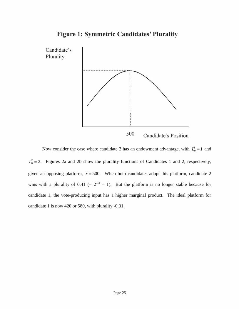
point is 1* 2* 500.x x The plurality function of either candidate, opposed by a candidate who
adopts the equilibrium platform, is reproduced graphically in Figure 1. This is a stable
equilibrium, since neither candidate can increase her plurality by a unilateral move. Notice too
that the plurality functions are smooth, with continuous first derivatives.
Page 25
Now consider the case where candidate 2 has an endowment advantage, with 1
0 1L and
2
0 2.L Figures 2a and 2b show the plurality functions of Candidates 1 and 2, respectively,
given an opposing platform, 500.x When both candidates adopt this platform, candidate 2
wins with a plurality of 0.41 (= 21/2
– 1). But the platform is no longer stable because for
candidate 1, the vote-producing input has a higher marginal product. The ideal platform for
candidate 1 is now 420 or 580, with plurality -0.31.

Page 26
Suppose candidate 1 moves to platform 1 420.x Candidate 2, still at 2 500,x would
have a plurality of 0.31 and could improve to 0.41 by matching candidate 1 at 2 420.x
Candidate 1’s plurality function when candidate 2 offers platform 420 is presented in Figure 3a.
Candidate 1 now maximizes her plurality by moving to 1 545.x Of course, candidate 2 can
reestablish his lead by matching candidate 1 at this new platform and the cycle will continue.
The pattern of cycling is presented in Figure 3b. Several points are illustrated by this example.
First, the plurality functions when candidates are not symmetrically endowed are no longer
smooth at the switching point where the candidate platforms are the same because the
contributions from supporters have different values for the two candidates. Second, the lesser-
endowed candidate will always seek to differentiate herself from the better-endowed candidate
and the latter will be inclined to follow. Third, the better-endowed candidate cannot be defeated
if he remains at 2 500x and permits a higher plurality for an optimizing opponent if he strays
from this platform. Finally, platforms cycle around 500, exploding outward when both
candidates are close to this platform and dampening back toward this platform when they are
farther away.

Page 27
Page 28
References
Adams, J. (1998). “Partisan Voting and Multiparty Spatial Competition: The Pressure for
Responsible Parties,” Journal of Theoretical Politics 10(1): 5-31.
Ansolabehere, S. and Iyenbgar, S. (1996) Going Negative: How Political Advertisements Shrink
and Polarize the Electorate. New York; The Free Press.
Ansolabehere, S. and Snyder, J. (2000). “Valance Politics and Equilibrium in Spatial Election
Models,” Public Choice 103: 327-36.
Aragones, E., and Palfrey, T. R. (2002). “Mixed Equilibrium in a Downsian Model with a
Favored Candidate,” Journal of Economic Theory 103 (March): 131-61.
Aragones, E., and Palfrey, T. R. (2004). “The Effect of Candidate Quality on Electoral
Equilibrium: An Experimental Study,” American Political Science Review 98 (February):
77-90.
Arrow, K.J. (1963). Social Choice and Individual Values. New York; Wiley, (second edition).
Ashworth, S. (2006). “Campaign Finance and Voter Welfare with Entrenched Incumbents,”
American Political Science Review 100 (February): 55-68.
Ball, R. (1999). “Discontinuity and Non-existence of Equilibrium in the Probabilistic Spatial
Voting Model,” Social Choice and Welfare 16: 533 - 555
Becker, G.S. (1983). “A Theory of Competition Among Pressure Groups for Political
Influence,” Quarterly Journal of Economics 98: 371-400.
Bental, B., and Ben-Zion, U. (1975). “Political Contribution and Policy – Some Extensions,”
Public Choice 24 (Winter): 1-12.
Page 29
Ben-Zion, U, and Eytan, Z. (1974). “On Money, Votes, and Policy in a Democratic Society,”
Public Choice 17 (Spring): 1-10.
Berger, M.M., Munger, M.C., and Pothoff, R.F. (2000). “The Downsian Model Predicts
Divergence,” Journal of Theoretical Politics 12(2): 228-240.
Black, D. (1958). The Theory of Committees and Elections. Cambridge; Cambridge Univ. Press.
de Condorcet (1785) Essai sur l’application de l’analyse a la probabilite des decisions rendue a la
pluralite des voix, Paris .
Cook, W.D., Kirby, M.J.L., and Mehndiratta, S.L. (1974). “Models for the Optimal Allocation
of Funds over N Constituencies During an Election Campaign,” Public Choice 20
(Winter): 1-16.
Coughlin, P.J. (1982). Pareto Optimality of Policy Proposals with Probabilistic Voting. Public
Choice39: 427-433.
Coughlin, P.J. (1986). Elections and Income Redistribution. Public choice 50: 27-99.
Coughlin, P.J. (1990). Majority Rule and Election Models. Journal of Economic Surveys 3, no. 2,
pp. 157-188.
Coughlin, P.J., (1991). Probabilistic Voting Theory. Cambridge, MA: Cambridge University
Press.
Coughlin, P.J. and Nitzan, S. (1981a). Electoral Outcomes with Probabilistic Voting and Nash
Social Welfare Maxima. Journal of Public Economics 15: 113-122.
Coughlin, P.J. and Nitzan, S. (1981b). Directional and Local Electoral Equilibria with
Probabilistic Voting. Journal of Economic Theory 24: 226-239.

Page 30
Coughlin, P.J., Mueller, D.C. and Murrell, P. (1990). Electoral Politics, Interest Groups, and the
Size of Government. Economic Inquiry 28:628-750.
Davis, M.L. and Porter, P.K. (1989). A Test for Pure or Apparent Ideology in Congressional
Voting, Public Choice 60: 101-112.
Davis, O.A., Hinich, M.J., and Ordeshook, P.C. (1970)”An Expository Development of a
Mathmatical Model of the Electoral Process,” American Political Science Review 64:
426-48.
Dodgson, C.L. (1876). A Method of Taking Votes on More than Two Issues. Oxford: Clarendon
Press.
Downs, Anthony. (1957). An Economic Theory of Democracy. New York: Harper & Row.
Enelow, J.M. and Hinich, M.J. (1981). “A New Approach to Voter Uncertainty in the Downsian
Spatial Model.” American Journal of Political Science 25: 483-493.
Enelow, James M., and Hinich, M.J. (1984). The Spatial Theory of Voting: An Introduction.
Cambridge: Cambridge Univ. Press.
Feld, S.L. and Gorfman, B. (1991). “Incumbency Advantage, Voter Loyalty and the Benefit of
the Doubt,” Journal of Theoretical Politics, 3(1): 115-37.
Feldman, A.M. and Lee, K.-M. (1988). Existence of Electoral Equilibria with Probabilistic
Voting. Journal of Public Economics 35: 205-227.
Gerber, A. (1998). “Estimating the Effect of Campaign Spending on Senate Election Outcomes
Using Instrumental Variables,” American Political Science Review 92 (June): 401-11.

Page 31
Goodman, J.C. (1976). The Market for Coercion: A Neoclassical Theory of the State. Columbia
University Dissertation, New York.
Goodman, J.C. (1980). A Note on Existence and Uniqueness of Equilibrium Points for Concave
N-person N-games. Notes and Points. Econometrica 48, no. 1: 251.
Goodman, J.C. and Porter, P.K. (1985). “Majority Voting and Pareto Optimality.” Public Choice
Vol. 46, No. 2, pp. 173-186.
Goodman, J.C. and Porter, P.K. (1988). “Theory of Competitive Regulatory Equilibrium.”
Public Choice Vol. 59, pp. 51-66.
Goodman, J.C. and Porter, P.K. (2004). “Political Equilibrium and the Provision of Public
Goods.” Public Choice Vol. 120, pp. 247-266.
Groseclose, T. (2001). “A Model of Candidate Location When One Candidate Has Valance
Advantage,” American Journal of Political Science 45(4): 862-86.
Hinich, M., Ledyard, J. and Ordeshook, P. (1972). Nonvoting and the Existence of Equilibrium
under Majority Rule. Journal of Economic Theory 4: 144-153.
Hinich, M., Ledyard J., Ordeshook, P. (1973). “A Theory of Electoral Equilibrium: A Spatial
Analysis Based on the Theory of Games.” J Polit 35: 154-193.
Hinich, M. (1977) “Equilibrium in Spatial Voting: The Median Voter Result is an Artifact.” J
Econ Theory 16: 209-219.
Hotelling, H. (1929). “Stability in Competition.” Econ. J. 39 (March): 41-57.
Kalt, J.P. and Zupan, M.A. (1984). “Capture and Ideology in the Economic Theory of Politics.”
American Economic Review 74: 279-300.

Page 32
______________________(1990). “The Apparent Ideological Behavior of Legislators: Testing
for Principle-Agent Slack in Political Institutions.” Journal of Law and Economics
33:103-31.
Kau, J. and Rubin, P. (1979). “Self-interest, Ideology, and Log-rolling in Congressional
Voting.” Journal of Law and Economics 22: 365-84.
Kirchgassner, G. (2000), “Probabilistic Voting and Equilibrium: An Impossibility Result.”
Public Choice, 103: 35-48.
Lafay, J.-D. (1993). The Silent Revolution of Probabilistic Voting. In A. Breton, G. Galeotti, P.
Salmon and R. Wintrobe (Eds.), Preferences and Democracy, 159-191. Dordrecht:
Kluwer.
Ledyard, J (1984). “The Pure Theory of Large Two-Candidate Elections.” Public Choice 44: 7-
41.
Lindbeck, A. and Weibull, J. (1987): “Balanced-budget Redistribution as the Outcome of
Political Competition.: Public Choice, 52: 273-97.
McKelvy, R., (1975), “Policy Related Voting and Electoral Equilibria,” Econometrica 43: 815-
44.
Mueller, D.C. (2003) Public Choice III. Cambridge, MA: Cambridge University Press.
Olson, M. (1965). The Logic of Collective Action. Cambridge, MA: Harvard University Press.
Ordeshook, P.C. (1971). Pareto Optimality and Electoral Competition. American Political
Science Review 65: 1141-1145.

Page 33
Ordeshook, P.C. and Shepsle, K.A. (Eds.) (1982). Political Equilibrium. Boston: Kluwer
Nijhoff Publishing.
Peltzman, S. (1984), Constituent Interest and Congressional Voting. Journal of Law and
Economics 20 (1): 181-210.
Prat, A. (2002). “Campaign Advertising and voter Welfare,” Review of Economic Studies 69:
999-1017.
Riker (1961). Voting and the Summation of Preferences: an Interpretive Bibliographic Review of
Selected Developments During the Last Decade. The American Political Science Review
55 (4): 900 – 911.
Riker (1982). The Two-party System and Duverger’s Law: an Essay on the History of Political
Science. The American Political Science Review 76, no. 4: 753-766
Rosen (1965). Existence and Uniqueness of Equilibrium Points for Concave N-person Games.
Econometrica 33, no. 3: 520 - 534.
Sandkoff and Mellos (1972). The Swing Ratio and Game Theory. The American Political
Science Review 66, no. 2: 551 – 554.
Schofield, N. (2003). “Valance Competition in the Spatial Stochastic Model,” Journal of
Theoretical Politics 15(4): 371-83.
Schofield, N. (2004). “Equilibrium in the Spatial ‘Valance’ Model of Politics,” Journal of
Theoretical Politics 16(4): 447-81.
Welch, W. (1974). The Economics of Campaign Funds. Public Choice 20: 83-97.

Page 34
Welch, W. (1980). The Allocation of Political Monies: Economic Interest Groups. Public Choice
35: 97-120.
Top Related