


Languages
Pages
Legal


INTEGER LINEAR PROGRAMMING - INTRODUCTION

Integer Linear Programming
a
11x
1+ a
12x
2+ ·
· ·+a
1nx
n b
1
Feasible Region: Z-Polyhedron (n dimensional)
max c1x1 +c2x2 + · · ·+ cnxn
s.t. a11x1 +a12x2 + · · ·+ a1nxn b1
. . ....
am1x1 +am2x2 + · · ·+ amnxn bm
x1, . . . , xn 2 Z
Integrality Constraint

Integer Linear Programming • Relaxation to a (real-valued) Linear Program • How does the LP relaxation answer relate to the ILP answer? • Integrality Gap
• Complexity of Integer Linear Programs • NP-Completeness • Some special cases of ILPs.
• Algorithms: • Branch-And-Bound • Gomory-Chvatal Cuts

INTEGER LINEAR PROGRAMMING: LP RELAXATION 1. Relax an ILP to an LP 2. Examples with same answers and different
answers. 3. Integrality gap.

Integer Linear Programming
a
11x
1+ a
12x
2+ ·
· ·+a
1nx
n b
1
Feasible Region: Z-Polyhedron (n dimensional)
max c1x1 +c2x2 + · · ·+ cnxn
s.t. a11x1 +a12x2 + · · ·+ a1nxn b1
. . ....
am1x1 +am2x2 + · · ·+ amnxn bm
x1, . . . , xn 2 Z

Integer Linear Program • Feasibility of ILP: • Integer feasible solution.
• Unbounded ILP: • Integer feasible solutions can achieve arbitrarily large values for the
objective.
max c1x1 +c2x2 + · · ·+ cnxn
s.t. a11x1 +a12x2 + · · ·+ a1nxn b1
. . ....
am1x1 +am2x2 + · · ·+ amnxn bm
x1, . . . , xn 2 Z

Linear Programming Relaxation
max c1x1 +c2x2 + · · ·+ cnxn
s.t. a11x1 +a12x2 + · · ·+ a1nxn b1
. . ....
am1x1 +am2x2 + · · ·+ amnxn bm
x1, . . . , xn 2 ZQ: What happens to the answer if we take away the integrality constraints?

Feasible Regions max c1x1 +c2x2 + · · ·+ cnxn
s.t. a11x1 +a12x2 + · · ·+ a1nxn b1
. . ....
am1x1 +am2x2 + · · ·+ amnxn bm
x1, . . . , xn 2 Z
ILP feasible region LP feasible region ✓

Case-1: Both LP and ILP are feasible.
Opt. Solution of ILP
Opt. Solution of LP relaxation

Case-I Optimal Objective of ILP ≤ Optimal solution of LP relaxation.
Opt. Solution of ILP

Example-1 Write down an example where LP optimum = ILP optimum

Example-2 Write down an example where the two optima differ
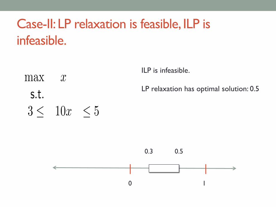
Case-II: LP relaxation is feasible, ILP is infeasible.
max x
s.t.3 10x 5
0 1
0.3 0.5
ILP is infeasible. LP relaxation has optimal solution: 0.5

Case III: ILP is infeasible, LP is unbounded. Example:
max y
3 10x 5
0 y
0.3 0.5
ILP is infeasible. LP relaxation is unbounded

ILP outcomes vs. LP relaxation outcomes
Infeasible Unbounded
Optimal
Infeasible Possible Impossible Impossible
Unbounded
Possible Possible Possible (*)
Optimal Possible Impossible Possible
Integer Linear Program (ILP)
LP Relaxation
(*) Impossible if ILP has rational coefficients

Summary (LP relaxation) • LP relaxation: ILP minus the integrality constraints.
• LP relaxation’s feasible region is a super-set of ILP feasible region.
• Analysis of various outcomes for ILP vs. outcomes for LP relaxations.

COMPLEXITY OF ILP

Polynomial Time Solvable Problems
Complexity of Integer Linear Programs Integer Linear Programming problems are NP-complete
Polynomial Time Solvable Problems
Non-determinstic Polynomial Time (NP)
Integer Linear Programming

Implications of P vs NP question • P=NP • Considered an unlikely possibility by experts. • In this case, we will be able to solve ILPs in polynomial time.
• P != NP • In this case, we can show a non-polynomial lower bound on the
complexity of solving ILPs.

Current State-of-the-art • We have some very good algorithms for solving ILPs • They perform well on some important instances. • But, they all have exponential worst-case complexity.
• Compared to LPs, • The largest ILPs that we can solve are a 1000-fold smaller.
• Two strategies: • Try to solve the ILP • Find approximate answers for some special ILP instances.

ILP AND COMBINATORIAL OPTIMIZATION Reducing 3-SAT to ILP

3-SAT Problem
x1, x2, x3, x4 Boolean Variables
(x1 OR x2 OR ¬x3)
(¬x2 OR ¬x4 OR x1)
(x1 OR x2 OR ¬x3)Find values for Boolean variables such that All the Clauses are True.
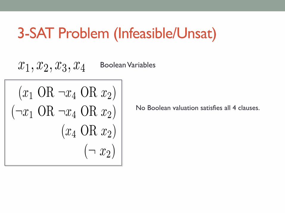
3-SAT Problem (Infeasible/Unsat)
x1, x2, x3, x4 Boolean Variables
(x1 OR ¬x4 OR x2)
(¬x1 OR ¬x4 OR x2)
(x4 OR x2)
(¬ x2)
No Boolean valuation satisfies all 4 clauses.

Reducing 3-SAT to ILP
x1, . . . , xn are Boolean variables.
C1 : (`1,1 OR `1,2 OR `1,3)...
. . .
Cm : (`m,1 OR `m,2 OR `m,3)
m Clauses.
`i,j stands for a variable xk or its negation ¬xk

ILP reduction.
xj ! yj 2 {0, 1} False = 0 True = 1
¬xj ⌘ (1� yj)
(x1 OR x2 OR ¬x5) ! y1 + y2 + (1� y5) � 1
Clauses Inequalities

Example-1
(x1 OR x2 OR ¬x3)
(¬x2 OR ¬x4 OR x1)
(x1 OR x2 OR ¬x3)
Convert this SAT problem to an ILP
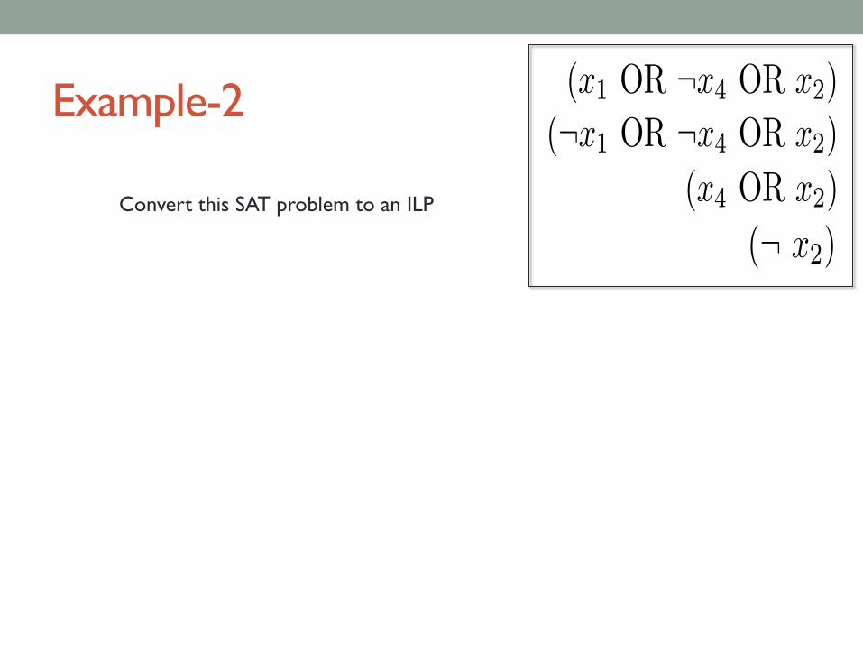
Example-2 (x1 OR ¬x4 OR x2)
(¬x1 OR ¬x4 OR x2)
(x4 OR x2)
(¬ x2)Convert this SAT problem to an ILP

LP RELAXATION VS. ILP RELAXATION

Claim LP relaxation’s answer can be arbitrarily larger than the ILP’s answer.
(0,0) (1,0)
( 12 ,K)
max x2
s.t x2 � 0
2Kx1 �x2 � 0
�2Kx1 �x2 � �2K
x1, x2 2 Z
.

ILP AND VERTEX COVER A flavor of approximation algorithms

Rounding Schemes • LP relaxation yields solutions with fractional parts.
• However, ILP asks for integer solution.
• In some cases, we can approximate ILP optimum by “rounding” • Take optimal solution of LP relaxation • Round the answer to an integer answer using rounding scheme. • Deduce something about the ILP optimal solution.

Vertex Cover Problem
1 2
4
3
5
87
6
Choose smallest subset of vertices Every edge must be “covered”
Eg, { 1, 2, 3, 5 } or {1, 2, 3, 7 }
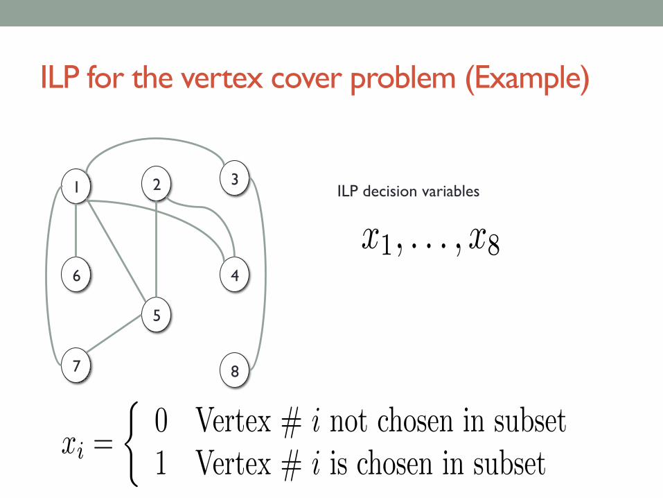
ILP for the vertex cover problem (Example)
1 2
4
3
5
87
6
x1, . . . , x8
xi =
⇢0 Vertex # i not chosen in subset
1 Vertex # i is chosen in subset
ILP decision variables

ILP for the vertex cover problem (Example)
1 2
4
3
5
87
6
min x1 + x2 + · · ·+ x8
s.t. x1 + x7 � 1 Edge: (1, 7)x1 + x6 � 1 Edge: (1, 6)x2 + x4 � 1
· · ·xi + xj � 1 (i, j) 2 E
· · ·x1 1...
x8 1x1, . . . , x8 � 0x1, . . . , x8 2 Z

Vertex Cover to ILP • Vertices {1,…, n} • Decision variables:
x1, . . . , xn xi 2 {0, 1}
minPn
i=1 xi
s.t. 0 xi 1 8 i 2 V
xi + xj � 1 8 (i, j) 2 E
xi 2 Z 8 i 2 V

LP relaxation of a vertex cover • Problem: we may get fractional solution.
1 2
4
3
5
87
6
x1 1x2 1x3
34
x4 0x5
56
x6 0x7
16
x814
Objective value: 4 But solution meaningless for vertex cover.

Rounding Scheme • Simple rounding scheme:
x
⇤i � 1
2 ! xi = 1Real-Optimal Solution is at least 0.5
Include vertex in the cover.
x
⇤i <
12 ! xi = 0

LP relaxation of a vertex cover • Problem: we may get fractional solution.
1 2
4
3
5
87
6
x1 1x2 1x3
34
x4 0x5
56
x6 0x7
16
x814
x1 1x2 1x3 1x4 0x5 1x6 0x7 0x8 0

Rounding Scheme Rounding scheme takes optimal fractional solution from LP relaxation and produces an integral solution.
x
⇤ rounding�������! ˆ
x
1. Does rounding always produces a valid vertex cover? 2. How does the rounded solution compare to the opt. solution?

Rounding Scheme Produces a Cover
x
⇤ rounding�������! ˆ
x
x
⇤i + x
⇤j � 1, for each (i, j) 2 E
x̂i = 1 or x̂j = 1 for each (i, j) 2 E
To Prove: The solution obtained after rounding covers every edge.

Rounding Scheme Approximation Guarantee
x
⇤ rounding�������! ˆ
x
Opt. Vertex Cover
LP relaxation Opt. Cost
Rounded Scheme
Cost
Fact: 2x
⇤i � x̂i for all vertices i.
2Pn
i=1 x⇤ �
Pni=1 x̂i
2 * (Cost of LP relaxation) � (Cost of Rounded Scheme Vertex Cover)

Approximation Guarantee • Theorem #1: Rounding scheme yields a vertex cover. • Cost of the solution obtained by rounding: C • Optimal vertex cover cost: C*
• Theorem #2: C* ≤ C ≤ 2 C*
• LP relaxation + rounding scheme: • 2-approximation for vertex cover!!

SOLVING ILP USING GLPK Specifying integer variables in Mathprog

GLPK integer solver • GLPK has a very good integer solver. • Uses branch-and-bound + Gomory cut techniques • We will examine these techniques soon.
• In this lecture, • Show how to solve (mixed) integer linear programs • Continue to use AMPL format.
• This is the best option for solving ILPs/MIPs

Example-1 (ILP)
min x1 +x2 +x3 +x4 +x5 +x6
x1 +x2 � 1x1 +x2 +x6 � 1
x3 +x4 � 1x3 +x4 +x5 � 1
x4 +x5 +x6 � 1x2 +x5 +x6 � 1
x1, x2, x3, x4, x5, x6 2 Z

Specifying variable type
var x; # specifies a real-valued decision variable var y integer; # specifies an integer variable var z binary; # specifies a binary variable

Example – I expressing in AMPL var x{1..6} integer; # Declare 6 integer variables minimize obj: sum{i in 1..6} x[i]; c1: x[1] + x[2] >= 1; c2: x[1] + x[2] + x[6] >= 1; c4: x[3] + x[4] >= 1; c5: x[3]+ x[4] + x[5] >= 1; c6: x[4] + x[5] + x[6] >= 1; c7: x[2] + x[5] + x[6] >= 1; solve; display{i in 1..6} x[i]; end
min x1 +x2 +x3 +x4 +x5 +x6
x1 +x2 � 1x1 +x2 +x6 � 1
x3 +x4 � 1x3 +x4 +x5 � 1
x4 +x5 +x6 � 1x2 +x5 +x6 � 1
x1, x2, x3, x4, x5, x6 2 Z

Example-1 Solving using GLPK Ø glpsol -- math ip1.math Display statement at line 25 x[1].val = 0 x[2].val = 1 x[3].val = 0 x[4].val = 1 x[5].val = 0 x[6].val = 0 Model has been successfully processed

Example -2 Vertex Cover Problem
source mathpuzzle.com
16

Vertex Cover to ILP • Vertices {1,…, n} • Decision variables:
x1, . . . , xn xi 2 {0, 1}
minPn
i=1 xi
s.t. 0 xi 1 8 i 2 V
xi + xj � 1 8 (i, j) 2 E
xi 2 Z 8 i 2 V

Vertex Cover AMPL (Model + Data) param n; var x {1..n} binary; # binary specifies that the variables are binary set E within {i in 1..n, j in 1..n: i < j}; # specify that the edges will be a set. # each edge will be entered as (i,j) where i < j minimize obj: sum{i in 1..n} x[i]; # minimize cost of the cover s.t. c{(i,j) in E}: x[i] + x[j] >= 1; solve; display{i in 1..n} x[i];
data; param n := 16; set E := (2,3) (3,5) (5,8) (4,16) (5,16) (8,14) (1,8) (4,12) (3,12) (4,14) (1,12) (2,14) (2,15) (1,15) (15,16) ; end;

Running GLPK … Ø glpsol -m vertexCover.model x[1].val = 0 x[2].val = 1 x[3].val = 0 x[4].val = 1 x[5].val = 1 x[6].val = 0 x[7].val = 0 x[8].val = 1 x[9].val = 0 x[10].val = 0 x[11].val = 0 x[12].val = 1 x[13].val = 0 x[14].val = 0 x[15].val = 1 x[16].val = 0
16

SOLVING ILPS IN MATLAB/OCTAVE

MATLAB Optimization Package • Supports solving binary integer programming problem • “bintprog function” • Same interface as linprog. • Except that all variables are assumed binary.
• Uses branch-and-bound • Not considered to be a good implementation.

CVX • Unfortunately, does not support integer programming in the
free version.
• Links to commercial tools Gurobi/MOSEK/CPLEX • Powerful state of the art integer solvers. • They make it available to academic users for free.
• We will continue to use GLPK for MATLAB/Octave.
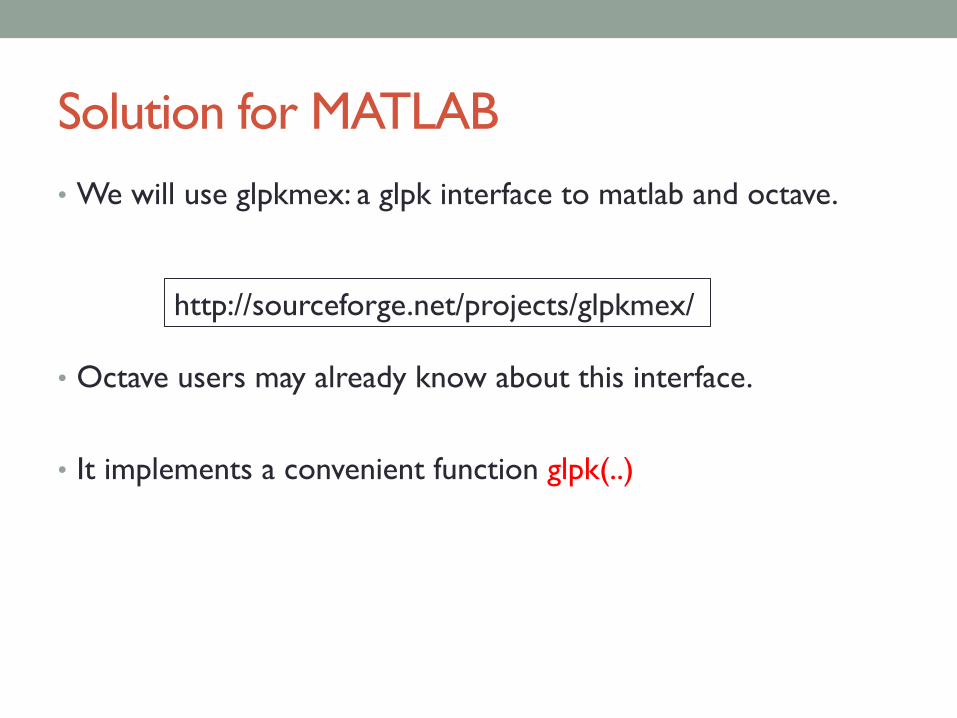
Solution for MATLAB • We will use glpkmex: a glpk interface to matlab and octave.
• Octave users may already know about this interface.
• It implements a convenient function glpk(..)
http://sourceforge.net/projects/glpkmex/

Over to matlab demo…
Top Related