


Languages
Pages
Legal

Integer factorization
Daniel J. Bernstein
2006.03.09
1
Table of contents
1. Introduction . . . . . . . . . . . . . . . . . . . . . . . . . . . . . . . . . . . . . . . . . . . . . . . . . . . . . . . . . . . . . . . . . 3
2. Overview . . . . . . . . . . . . . . . . . . . . . . . . . . . . . . . . . . . . . . . . . . . . . . . . . . . . . . . . . . . . . . . . . . . . 5
The costs of basic arithmetic . . . . . . . . . . . . . . . . . . . . . . . . . . . . . . . . . . . . . . . . . . . . . . . 7
3. Multiplication . . . . . . . . . . . . . . . . . . . . . . . . . . . . . . . . . . . . . . . . . . . . . . . . . . . . . . . . . . . . . . . 7
4. Division and greatest common divisor . . . . . . . . . . . . . . . . . . . . . . . . . . . . . . . . . . . . . . . . 8
5. Sorting . . . . . . . . . . . . . . . . . . . . . . . . . . . . . . . . . . . . . . . . . . . . . . . . . . . . . . . . . . . . . . . . . . . . . . 9
Finding small factors of one integer . . . . . . . . . . . . . . . . . . . . . . . . . . . . . . . . . . . . . . 11
6. Trial division . . . . . . . . . . . . . . . . . . . . . . . . . . . . . . . . . . . . . . . . . . . . . . . . . . . . . . . . . . . . . . . 11
7. Early aborts . . . . . . . . . . . . . . . . . . . . . . . . . . . . . . . . . . . . . . . . . . . . . . . . . . . . . . . . . . . . . . . . 13
8. The rho method . . . . . . . . . . . . . . . . . . . . . . . . . . . . . . . . . . . . . . . . . . . . . . . . . . . . . . . . . . . . 15
9. The p − 1 method . . . . . . . . . . . . . . . . . . . . . . . . . . . . . . . . . . . . . . . . . . . . . . . . . . . . . . . . . . 17
10. The p + 1 method . . . . . . . . . . . . . . . . . . . . . . . . . . . . . . . . . . . . . . . . . . . . . . . . . . . . . . . . . 19
11. The elliptic-curve method . . . . . . . . . . . . . . . . . . . . . . . . . . . . . . . . . . . . . . . . . . . . . . . . . 20
Finding small factors of many integers . . . . . . . . . . . . . . . . . . . . . . . . . . . . . . . . . . . 24
12. Consecutive integers: sieving . . . . . . . . . . . . . . . . . . . . . . . . . . . . . . . . . . . . . . . . . . . . . . 24
13. Consecutive polynomial values: sieving revisited . . . . . . . . . . . . . . . . . . . . . . . . . . . 28
14. Arbitrary integers: exploiting fast multiplication . . . . . . . . . . . . . . . . . . . . . . . . . . . 28
Finding large factors of one integer . . . . . . . . . . . . . . . . . . . . . . . . . . . . . . . . . . . . . . . 32
15. The Q sieve . . . . . . . . . . . . . . . . . . . . . . . . . . . . . . . . . . . . . . . . . . . . . . . . . . . . . . . . . . . . . . . 32
16. The linear sieve . . . . . . . . . . . . . . . . . . . . . . . . . . . . . . . . . . . . . . . . . . . . . . . . . . . . . . . . . . . 36
17. The quadratic sieve. . . . . . . . . . . . . . . . . . . . . . . . . . . . . . . . . . . . . . . . . . . . . . . . . . . . . . . .37
18. The number-field sieve. . . . . . . . . . . . . . . . . . . . . . . . . . . . . . . . . . . . . . . . . . . . . . . . . . . . .39
References . . . . . . . . . . . . . . . . . . . . . . . . . . . . . . . . . . . . . . . . . . . . . . . . . . . . . . . . . . . . . . . . . . . 40
Index . . . . . . . . . . . . . . . . . . . . . . . . . . . . . . . . . . . . . . . . . . . . . . . . . . . . . . . . . . . . . . . . . . . . . . . . .53
D. J. Bernstein, Integer factorization 2 2006.03.09

1 Introduction
1.1 Factorization problems. “The problem of distinguishing prime numbers from
composite numbers, and of resolving the latter into their prime factors, is known
to be one of the most important and useful in arithmetic,” Gauss wrote in his
Disquisitiones Arithmeticae in 1801. “The dignity of the science itself seems to
require that every possible means be explored for the solution of a problem so
elegant and so celebrated.”
But what exactly is the problem? It turns out that there are many different
factorization problems, as discussed below.
1.2 Recognizing primes; finding prime factors. Do we want to distinguish prime
numbers from composite numbers? Or do we want to find all the prime factors of
composite numbers?
These are quite different problems. Imagine, for example, that someone gives
you a 10000-digit composite number. It turns out that you can use “Artjuhov’s
generalized Fermat test”—the “sprp test”—to quickly write down a reasonably
short proof that the number is in fact composite. However, unless you’re extremely
lucky, you won’t be able to find all the prime factors of the number, even with
today’s state-of-the-art factorization methods.
1.3 Proven output; correct output. Do we care whether the answer is accompanied
by a proof? Is it good enough to have an answer that’s always correct but not
accompanied by a proof? Is it good enough to have an answer that has never been
observed to be incorrect?
Consider, for example, the “Baillie-Pomerance-Selfridge-Wagstaff test”: if n ∈3 + 40Z is a prime number then 2(n−1)/2 + 1 and x(n+1)/2 + 1 are both zero in
the ring (Z/n)[x]/(x2 − 3x + 1). Nobody has been able to find a composite n ∈3+40Z satisfying the same condition, even though such n’s are conjectured to exist.
(Similar comments apply to arithmetic progressions other than 3 + 40Z.) If both
2(n−1)/2 + 1 and x(n+1)/2 + 1 are zero, is it unacceptable to claim that n is prime?
1.4 All prime divisors; one prime divisor; etc. Do we actually want to find all
the prime factors of the input? Or are we satisfied with one prime divisor? Or any
factorization?
More than 70% of all integers n are divisible by 2 or 3 or 5, and are therefore
very easy to factor if we’re satisfied with one prime divisor. On the other hand,
some integers n have the form pq where p and q are primes; for these integers n,
finding one factor is just as difficult as finding the complete factorization.
1.5 Small prime divisors; large prime divisors. Do we want to be able to find the
D. J. Bernstein, Integer factorization 3 2006.03.09
prime factors of every integer n? Or are we satisfied with an algorithm that gives
up when n has large prime factors?
Some algorithms don’t seem to care how large the prime factors are; they
aren’t the best at finding small primes but they compensate by finding large
primes at the same speed. Example: “The Pollard-Buhler-Lenstra-Pomerance-
Adleman number-field sieve” is conjectured to find the prime factors of n using
exp((64/9 + o(1))1/3(log n)1/3(log log n)2/3) bit operations.
Other algorithms are much faster at finding small primes—let’s say primes in the
range {2, 3, . . . , y}, where y is a parameter chosen by the user. Example: “Lenstra’s
elliptic-curve method” is conjectured to find all of the small prime factors of n using
exp√
(2 + o(1))(log y) log log y multiplications (and similar operations) of integers
smaller than n. See Section 11.1.
1.6 Typical inputs; worst-case inputs; etc. More generally, consider an algorithm
that tries to find the prime factors of n, and that has different performance (different
speed; different success chance) for different inputs n. Are we interested in the
algorithm’s performance for typical inputs n? Or its average performance over all
inputs n? Or its performance for worst-case inputs n, such as integers chosen by
cryptographers to be difficult to factor?
Consider, as an illustration, the “Schnorr-Lenstra-Shanks-Pollard-Atkin-Rickert
class-group method.” This method was originally conjectured to find all the prime
factors of n using exp√
(1 + o(1))(logn) log log n bit operations. The conjecture
was later modified: the method seems to run into all sorts of trouble when n is
divisible by the square of a large prime.
1.7 Conjectured speeds; proven bounds. Do we compare algorithms according to
their conjectured speeds? Or do we compare them according to proven bounds?
The “Schnorr-Seysen-Lenstra-Lenstra-Pomerance class-group method” devel-
oped in [125], [129], [79], and [87] has been proven to find all prime factors of
n using at most exp√
(1 + o(1))(logn) log log n bit operations. The number-field
sieve is conjectured to be much faster, once n is large enough, but we don’t even
know how to prove that the number-field sieve works for every n, let alone that it’s
fast.
1.8 Serial; parallel. How much parallelism do we allow in our algorithms?
One variant of the number-field sieve uses L1.18563...+o(1) seconds on a machine
costing L0.79042...+o(1) dollars. Here L = exp((log n)1/3(log log n)2/3). The machine
contains L0.79042...+o(1) tiny parallel CPUs carrying out a total of L1.97605...+o(1)
bit operations. The price-performance ratio of this computation is L1.97605...+o(1)
dollar-seconds. This variant is designed to minimize price-performance ratio.
Another variant—watch the first two exponents of L here—uses L2.01147...+o(1)
seconds on a serial machine costing L0.74884...+o(1) dollars. The machine contains
D. J. Bernstein, Integer factorization 4 2006.03.09
L0.74884...+o(1) bytes of memory and a single serial CPU carrying out L2.01147...+o(1)
bit operations. The price-performance ratio of this computation is L2.76031...+o(1)
dollar-seconds. This variant is designed to minimize price-performance ratio for
serial computations.
Another variant—watch the last two exponents of L here—uses L1.90188...+o(1)
seconds on a serial machine costing L0.95094...+o(1) dollars. The machine contains
L0.95094...+o(1) bytes of memory and a single serial CPU carrying out L1.90188...+o(1)
bit operations. The price-performance ratio of this computation is L2.85283...+o(1)
dollar-seconds. This variant is designed to minimize the number of bit operations.
1.9 One input; multiple inputs. Do we want to find the prime factors of just a single
integer n? Or do we want to solve the same problem for many integers n1, n2, . . .?
Or do we want to solve the same problem for as many of n1, n2, . . . as possible?
One might guess that the most efficient way to handle many inputs is to handle
each input separately. But “sieving” finds the small factors of many consecutive
integers n1, n2, . . . with far fewer bit operations than handling each integer sepa-
rately; see Section 12.1. Furthermore, recent factorization methods have removed
the words “consecutive” and “small”; see, e.g., Sections 14.1 and 15.8.
2 Overview
2.1 The primary factorization problem. Even a year-long course can’t possibly
cover all the interesting factorization methods in the literature. In my lectures
at the Arizona Winter School I’m going to focus on “congruence-combination”
factorization methods, specifically the number-field sieve, which holds the speed
records for real-world factorizations of worst-case inputs such as RSA moduli.
Here’s how this fits into the spectrum of problems considered in Section 1:
• I don’t merely want to know that the input n is composite; I want to know
its prime factors.
• I’m much less concerned with proving the primality of the factors than with
finding the factors in the first place.
• I want an algorithm that works well for every n—in particular, I don’t want
to give up on n’s with large prime factors.
• I want to factor n as quickly as possible. I’m willing to sacrifice proven bounds
on performance in favor of reasonable conjectures.
• I’m interested in parallelism to the extent that I have parallel machines.
• I might be interested in speedups from factoring many integers at once, but
my primary concern is the already quite difficult problem of factoring a single
large integer.
D. J. Bernstein, Integer factorization 5 2006.03.09

Sections 15 through 18 in these notes discuss congruence-combination methods,
starting with the Q sieve and culminating with the number-field sieve.
2.2 The secondary factorization problem. A secondary factorization problem
of a quite different flavor turns out to be a critical subroutine in “congruence-
combination” algorithms. What these algorithms do is
• write down many “congruences” related to the integer n being factored;
• search for “fully factored” congruences; and then
• combine the fully factored congruences into a “congruence of squares” used
to factor n.
The secondary factorization problem is the middle step here, the search for “fully
factored” congruences. This step involves many inputs, not just one; it involves
inputs typically much smaller than n; inputs with large prime factors can be, and
are, thrown away; the problem is to find small factors as quickly as possible.
In my lectures at the Arizona Winter School I’ll present the state of the art in
small-factors algorithms, including the elliptic-curve method and a newer method
relying on the Schonhage-Strassen FFT-based algorithm for multiplying billion-
digit integers.
The student project attached to this course at the Arizona Winter School is
to actually use computers to factor a bunch of integers! The project will take the
secondary perspective: there are many integers to factor; integers with large prime
factors—integers that aren’t “smooth”—are thrown away; the problem is to find
small factors as quickly as possible. We’re going to write real programs, see which
programs are fastest, and see which programs are most successful at finding factors.
Sections 6 through 14 in these notes discuss methods to find small factors of
many inputs. One approach is to handle each input separately; Sections 6 through
11 discuss methods to find small factors of one input. Sections 12 through 14 discuss
methods that gain speed by handling many inputs simultaneously.
2.3 Other resources. There are several books presenting integer-factorization algo-
rithms: Knuth’s Art of computer programming, Section 4.5.4; Cohen’s Course in
computational algebraic number theory, Chapter 10; Riesel’s Prime numbers and
computer methods for factorization; and, newest and generally most comprehen-
sive, the Crandall-Pomerance book Prime numbers: a computational perspective.
All of these books also cover the problems of recognizing prime numbers and proving
primality. The Crandall-Pomerance book is highly recommended.
D. J. Bernstein, Integer factorization 6 2006.03.09
The costs of basic arithmetic
3 Multiplication
3.1 Bit operations. One can multiply two b-bit integers using Θ(b lg 2b lg lg 4b) bit
operations. Often I’ll state speeds in less detail to focus on the exponent of b:
multiplication uses b1+o(1) bit operations.
More precisely: For each integer b ≥ 1, there is a circuit using Θ(b lg 2b lg lg 4b)
bit operations to multiply two integers in{
0, 1, . . . , 2b − 1}
, when each input is
represented in the usual way as a b-bit string and the output is represented in the
usual way as a 2b-bit string. A “bit operation” means, by definition, the 2-bit-to-
1-bit function x, y 7→ 1 − xy; a “circuit” is a chain of bit operations.
This means that multiplication is not much slower than addition. Addition also
uses b1+o(1) bit operations: more precisely, Θ(b) bit operations. For comparison,
the most obvious multiplication methods use Θ(b2) bit operations; multiplication
methods using Θ(b lg 2b lg lg 4b) bit operations are often called “fast multiplication.”
The bound b1+o(1) for multiplication was first achieved by Toom in [139]. The
bound O(b lg 2b lg lg 4b) was first achieved by Schonhage and Strassen in [128], using
the fast Fourier transform (FFT). See my paper [20, Sections 2–4] for an exposition
of the Schonhage-Strassen circuit.
3.2 Instructions. One can view the multiplication circuit in Section 3.1 as a series
of Θ(b lg 2b lg lg 4b) instructions for a machine that reads bits from various memory
locations, performs simple operations on those bits, and writes the bits back to
various memory locations. The circuit is “uniform”: this means that one can,
given b, easily compute the series of instructions.
The instruction counts in these notes don’t take account of the possibility of
changing the representation of integers to exploit more powerful instructions. For
example, in many models of computation, a single instruction can operate on a
w-bit “word” with w ≥ lg 2b; this instruction reduces the costs of both addition
and multiplication by a factor of w if integers are appropriately recoded. Machine-
dependent speedups often save time in real factorizations.
3.3 Serial price-performance ratio. The b1+o(1) instructions in Section 3.2 take
b1+o(1) seconds on a serial machine costing b1+o(1) dollars for b1+o(1) bits of mem-
ory; the price-performance ratio is b2+o(1) dollar-seconds. More precisely, the
Θ(b lg 2b lg lg 4b) instructions take Θ(b lg 2b lg lg 4b) seconds on a serial machine with
Θ(b lg 2b) bits of memory; the price-performance ratio is Θ(b2(lg 2b)2 lg lg 4b) dollar-
seconds.
D. J. Bernstein, Integer factorization 7 2006.03.09
One can and should object to the notion that an instruction finishes in Θ(1)
seconds. In any realistic model of a two-dimensional computer, b1+o(1) bits of
memory are laid out in a b0.5+o(1) × b0.5+o(1) mesh, and random access to the
mesh has a latency of b0.5+o(1) seconds; transmitting signals across a distance of
b0.5+o(1) meters necessarily takes b0.5+o(1) seconds. However, in this computation,
the memory accesses can be pipelined: b0.5+o(1) memory accesses take place during
the same b0.5+o(1) seconds, hiding the latency of each access.
3.4 Parallel price-performance ratio. A better-designed multiplication machine of
size b1+o(1) takes just b0.5+o(1) seconds, asymptotically much faster than any serial
multiplication machine of the same size. The price-performance ratio is b1.5+o(1)
dollar-seconds.
The critical point here is that a properly designed machine of size b1+o(1) can
carry out b1+o(1) instructions in parallel. In b0.5+o(1) seconds, one can do much
more than access b0.5+o(1) memory locations: all b1+o(1) parallel processors can
exchange data with each other. See Section 5.4 below.
Details of a b-bit multiplication machine achieving this performance, size b1+o(1)
and b0.5+o(1) seconds, were published by Brent and Kung in [33, Section 4]. Brent
and Kung also proved that the limiting exponent 0.5 is optimal for an extremely
broad class of 2-dimensional multiplication machines of size b1+o(1).
4 Division and greatest common divisor
4.1 Instructions. One can compute the quotient and remainder of two b-bit integers
using b1+o(1) instructions: more precisely, Θ(b lg 2b lg lg 4b) instructions, within a
constant factor of the cost of multiplication.
One can compute the greatest common divisor gcd{x, y} of two b-bit integers x, y
using b1+o(1) instructions: more precisely, Θ(b(lg 2b)2 lg lg 4b) instructions, within a
logarithmic factor of the cost of multiplication.
Recall that the multiplication instructions described in Section 3.2 simulate
the bit operations in a circuit. The same is not true for division and gcd: the
instructions for division and gcd use not only bit operations but also data-dependent
branches.
The bound b1+o(1) for division was first achieved by Cook in [46, pages 77–86].
The bound Θ(b lg 2b lg lg 4b) was first achieved by Brent in [28]. See my paper [20,
Sections 6–7] for an exposition.
The bound b1+o(1) for gcd was first achieved by Knuth in [76]. The bound
Θ(b(lg 2b)2 lg lg 4b) was first achieved by Schonhage in [127]. See my paper [20,
Sections 21–22] for an exposition.
D. J. Bernstein, Integer factorization 8 2006.03.09

4.2 Bit operations. One can compute the quotient, remainder, and greatest common
divisor of two b-bit integers using b1+o(1) bit operations. I’m not aware of any
literature stating, let alone minimizing, a more precise upper bound.
4.3 Serial price-performance ratio. Division and gcd, like multiplication, use
b1+o(1) bits of memory. The b1+o(1) memory accesses in a serial computation can
be pipelined, with more effort than in Section 3.3, to take b1+o(1) seconds. The
price-performance ratio is b2+o(1) dollar-seconds.
4.4 Parallel price-performance ratio. Division, like multiplication, can be heavily
parallelized. A properly designed division machine of size b1+o(1) takes just b0.5+o(1)
seconds, asymptotically much faster than any serial division machine of the same
size. The price-performance ratio is b1.5+o(1) dollar-seconds.
Parallelizing a gcd computation is a famous open problem. Every polynomial-
sized gcd machine in the literature takes at least b1+o(1) seconds. The best known
price-performance ratio is b2+o(1) dollar-seconds.
5 Sorting
5.1 Bit operations. One can sort n integers, each having b bits, into increasing
order using Θ(bn lg 2n) bit operations: more precisely, using a circuit of Θ(n lg 2n)
comparisons, each comparison consisting of Θ(b) bit operations.
History: Two sorting circuits with n1+o(1) comparisons, specifically Θ(n(lg 2n)2)
comparisons, were introduced by Batcher in [15]; an older circuit, “Shell sort,”
was later proven to achieve the same Θ(n(lg 2n)2) comparisons. A circuit with
Θ(n lg 2n) comparisons was introduced by by Ajtai, Komlos, and Szemeredi in [6].
5.2 Instructions. One can sort n integers, each having b bits, into increasing order
using Θ(bn) instructions. Note the lg factor improvement compared to Section 5.1;
instructions are slightly more powerful than bit operations because they can use
variables as memory addresses.
History: “Merge sort,” “heap sort,” et al. use O(n lg 2n) compare-exchange
steps, where each compare-exchange step uses Θ(b) instructions. “Radix-2 sort” is
not comparison-based and uses only Θ(bn) instructions. All of these algorithms are
standard.
5.3 Serial price-performance ratio. The Θ(bn) instructions in Section 5.2 are easily
pipelined to take Θ(bn) seconds on a serial machine with Θ(bn) bits of memory.
The price-performance ratio is Θ(b2n2) dollar-seconds.
D. J. Bernstein, Integer factorization 9 2006.03.09
5.4 Parallel price-performance ratio. A better-designed sorting machine of size
Θ(bn) takes just Θ(bn1/2) seconds, much faster than any serial sorting machine of
the same size. The price-performance ratio is Θ(b2n3/2) seconds.
History: Thompson and Kung in [138] showed that an n1/2 × n1/2 mesh of
small processors can sort n numbers with Θ(n1/2) adjacent compare-exchange steps.
Schnorr and Shamir in [126] presented an algorithm using (3 + o(1))n1/2 adjacent
compare-exchange steps. Schimmler in [124] presented a simpler algorithm using
(8 + o(1))n1/2 adjacent compare-exchange steps. I recommend that you start with
Schimmler’s algorithm if you’re interested in learning parallel sorting algorithms.
D. J. Bernstein, Integer factorization 10 2006.03.09

Finding small factors of one integer
6 Trial division
6.1 Introduction. “Trial division” tries to factor a positive integer n by checking
whether n is divisible by 2, checking whether n is divisible by 3, checking whether
n is divisible by 4, checking whether n is divisible by 5, and so on. Trial division
stops after checking whether n is divisible by y; here y is a positive integer chosen
by the user.
If n is not divisible by 2, 3, 4, . . . , d − 1, but turns out to be divisible by d,
then trial division prints d as output and recursively attempts to factor n/d. The
divisions by 2, 3, 4, . . . , d−1 can be skipped inside the recursion: n/d is not divisible
by 2, 3, 4, . . . , d − 1.
6.2 Example. Consider the problem of factoring n = 314159265. Trial division with
y = 10 performs the following computations:
• 314159265 is not divisible by 2;
• 314159265 is divisible by 3, so replace it with 314159265/3 = 104719755 and
print 3;
• 104719755 is divisible by 3, so replace it with 104719755/3 = 34906585 and
print 3 again;
• 34906585 is not divisible by 3;
• 34906585 is not divisible by 4;
• 34906585 is divisible by 5, so replace it with 6981317 and print 5;
• 6981317 is not divisible by 5;
• 6981317 is not divisible by 6;
• 6981317 is not divisible by 7;
• 6981317 is not divisible by 8;
• 6981317 is not divisible by 9;
• 6981317 is not divisible by 10.
This computation has revealed that 314159265 is 3 times 3 times 5 times 6981317;
the factorization of 6981317 is unknown.
6.3 Improvements. Each divisor d found by trial division is prime. Trial division
will never output 6, for example. One can exploit this by skipping composites
and checking only divisibility by primes; there are only about y/log y primes in
{2, 3, 4, . . . , y}.
D. J. Bernstein, Integer factorization 11 2006.03.09

If n has no prime divisor in {2, 3, . . . , d − 1}, and 1 < n < d2, then n must be
prime; there is no point in checking divisibility of n by d or anything larger. One
easy way to exploit this is by stopping trial division—and printing n as output—if
the quotient bn/dc is smaller than d. One can also use more sophisticated tests to
check for primes n larger than d2.
6.4 Speed. Trial division performs at most y − 1 + r divisions if it discovers r factors
of n. Each division is a division of n by an integer in {2, 3, 4, . . . , y}. One can safely
ignore the r here: r cannot be larger than lg n, and normally y is chosen much
larger than lg n.
Skipping composites incurs the cost of enumerating the primes below y—using,
for example, the techniques discussed in Section 12.3—but reduces the number of
divisions to about y/log y.
Stopping trial division at d when bn/dc < d can eliminate many more divisions,
depending on n, at the minor cost of a comparison.
Checking for a larger prime n can also eliminate many more divisions. The time
for a primality test is, for an average n, comparable to roughly lg n divisions, so it
doesn’t add a noticeable cost if it’s carried out after, e.g., 10 lg n divisions.
6.5 Effectiveness. Trial division—with the bn/dc < d improvement—is guaranteed to
find the complete factorization of n if y2 > n. In other words, trial division—with
the bn/dc < d improvement, and skipping composites—is guaranteed to succeed
with at most about√
n/log√
n divisions. For example, if n ≈ 2100, then trial
division is guaranteed to succeed with at most about 244.9 divisions.
Often trial division succeeds with a much smaller value of y. For example,
if y = 10, then trial division will completely factor any integer n of the form
2a3b5c7d; there are about (log x)4/24(log 2)(log 3)(log 5)(log 7) such integers n in
the range [1, x]. Trial division will also completely factor any integer n of the form
2a3b5c7dp where p is one of the 21 primes between 11 and 100; there are about
21(logx)4/24(log 2)(log 3)(log 5)(log 7) such integers n in the range [1, x]. There
are, for example, millions of integers n below 2100 that will be factored by trial
division with y = 10.
6.6 Definition of smoothness. Integers n that factor completely into primes ≤ y
(equivalently, that factor completely into integers ≤ y; equivalently, that have no
prime divisors > y) are called “y-smooth.”
Integers n that factor completely into primes ≤ y, except possibly for one prime
≤ y2, are called “(y, y2)-semismooth.” These integers are completely factored by
trial division up through y.
There’s a series of increasingly incomprehensible notations for more complicated
factorization conditions.
D. J. Bernstein, Integer factorization 12 2006.03.09
6.7 The standard smoothness estimate. There are roughly x/uu positive integers
n ≤ x that are x1/u-smooth, i.e., that are products of powers of primes ≤ x1/u.
For example, there are roughly 290/33 positive integers n ≤ 290 that are 230-
smooth, and there are roughly 2300/1010 positive integers n ≤ 2300 that are 230-
smooth. All of these integers are completely factored by trial division with y = 230,
i.e., with about 230/log 230 ≈ 225.6 divisions.
The uu formula isn’t extremely accurate. More careful calculations show that a
uniform random positive integer n ≤ 2300—“uniform” means that each possibility
is chosen with the same probability—has only about 1 chance in 3.3 · 1010 of being
230-smooth, not 1 chance in 1010. But the uu formula is in the right ballpark.
7 Early aborts
7.1 Introduction. Here is a method that tries to completely factor n into small primes:
• Use trial division with primes ≤ 215 to find some small factors of n, along
with the unfactored part n1 = n/those factors.
• Give up if n1 > 2100. This is an example of an “early abort.”
• Use trial division with primes ≤ 220 to find small factors of n1.
• Give up if n1 is not completely factored. This is a “final abort.”
Of course, the second trial-division step can skip primes ≤ 215.
More generally, given parameters y1 ≤ y2 ≤ · · · ≤ yk and A1 ≥ A2 ≥ · · · ≥Ak−1, one can try to completely factor n as follows:
• Use trial division with primes ≤ y1 to find some small factors of n, along with
the unfactored part n1.
• Give up if n1 > A1.
• Use trial division with primes ≤ y2 to find some small factors of n1, along
with the unfactored part n2.
• Give up if n2 > A2.
• . . .
• Use trial division with primes ≤ yk to find some small factors of nk−1, along
with the unfactored part nk.
• Give up if nk is not completely factored.
This is called “trial division with k − 1 early aborts.”
In subsequent sections we’ll see several alternatives to trial division: the rho
method, the p − 1 method, etc. Early aborts combine all of these methods, with
various parameter choices, into a grand unified method. What’s interesting is that
D. J. Bernstein, Integer factorization 13 2006.03.09
the cost-effectiveness curve of the grand unified method is considerably better than
all of the curves for the original methods.
7.2 Speed. There’s a huge parameter space for trial division with multiple early aborts.
How do we choose the prime bounds y1, y2, . . . and the aborts A1, A2, . . .?
Define T (y) as the average cost of trial division with primes ≤ y. The average
cost of multiple-early-abort trial division is then T (y1)+ p1T (y2)+ p1p2T (y3)+ · · ·where p1 is the probability that n survives the first abort, p1p2 is the probability
that n survives the first two aborts, etc.
One can choose the aborts to roughly balance the summands T (y1), p1T (y2),
p1p2T (y3), etc.: e.g., to have p1 ≈ T (y1)/2T (y2), to have p2 ≈ T (y2)/2T (y3), etc.,
so that the total cost is only about 2T (y1). Given many n’s, one can simply look
at the smallest ni’s and keep a fraction pi ≈ T (yi)/2T (yi+1) of them; one does not
need to choose Ai in advance.
What about the prime bounds y1, y2, . . .? An easy answer is to choose the
prime bounds in geometric progression: y1 = y1/k, y2 = y2/k, y3 = y3/k, and so on
through yk = yk/k = y. The total cost is then about 2T (y1/k). The user simply
needs to choose y, the final prime bound, and k, the number of aborts.
What about the alternatives to trial division that we’ll see later: rho, p − 1,
etc.? We can simply redefine T (y) as the average cost of our favorite method to find
primes ≤ y, and then proceed as above. The total cost will still be approximately
2T (y1/k), but most pi’s will be larger, allowing more n’s to survive the aborts and
improving the effectiveness of the algorithm.
These choices of yi and Ai are certainly not optimal, but Pomerance’s analysis
in [110, Section 4], and the empirical analysis in [122], shows that they’re in the
right ballpark.
7.3 Effectiveness. Assume that n is a uniform random integer in the range [1, x].
Recall from Section 6.7 that n is y-smooth with probability roughly 1/uu if y = x1/u.
The cost-effectiveness ratio for trial division with primes ≤ y, without any early
aborts, is roughly uuT (y).
The chance of n being completely factored by multiple-early-abort trial division,
with the parameter choices discussed in Section 7.2, is smaller than 1/uu by a factor
of roughly√
T (yk)/T (y1) =√
T (y)/T (y1/k). But the cost is reduced by a much
larger factor, namely T (y)/2T (y1/k). The cost-effectiveness ratio improves from
roughly uuT (y) to roughly 2uu√
T (y)T (y1/k).
The ideas behind these estimates are due to Pomerance in [110, Section 4].
I’ve gone to some effort to extract comprehensible formulas out of Pomerance’s
complicated formulas.
7.4 Punctured early aborts. Recall the first example of an early abort from Section
7.1: trial-divide n with primes ≤ 215; abort if the remaining part n1 exceeds 2100;
D. J. Bernstein, Integer factorization 14 2006.03.09
trial-divide n1 with primes ≤ 220.
There is no point in keeping n1 if it is between 220 and 230, or between 240 and
245: if n is 220-smooth then n1 is a product of primes between 215 and 220. There’s
also very little point in keeping n1 if, for example, it’s only slightly below 240. The
lack of prime factors below 215 means that the smallest integers are not the integers
most likely to be smooth.
I’m not aware of any analysis of the speedup produced by this idea.
8 The rho method
8.1 Introduction. Define ρ1, ρ2, ρ3, . . . by the recursion ρi+1 = ρ2i + 10, starting from
ρ1 = 1. The “rho method” tries to find a nontrivial factor of n by computing
gcd{n, (ρ2 − ρ1)(ρ4 − ρ2)(ρ6 − ρ3) · · · (ρ2z − ρz)};
here z is a parameter chosen by the user.
There’s nothing special about the number 10. The “randomized rho method”
replaces 10 with a uniform random element of {3, 4, . . . , n − 3}.We’ll see that the rho method with z ≈ √
y is about as effective as trial division
with all primes ≤ y; see Section 8.5. We’ll also see that the rho method takes about
4z ≈ 4√
y multiplications modulo n; see Section 8.4. This is faster than y/log y
divisions if y is not very small.
The rho method was introduced by Pollard in [107]. The name “rho” comes
from the shape of the Greek letter ρ; the shape is often helpful in visualizing the
graph with edges ρi mod p 7→ ρi+1 mod p, where p is a prime.
8.2 Example. The rho method, with z = 3, calculates ρ2 − ρ1 = 10; ρ4 − ρ2 = 17160;
ρ6 − ρ3 = 86932542660248880; and finally gcd{n, 10 · 17160 · 86932542660248880}.To understand why this is effective, observe that 10·17160·86932542660248880 =
28 · 35 · 53 · 7 · 11 · 13 · 17 · 53 · 71 · 101 · 191 · 1553. The differences ρ2i − ρi constructed
in the rho method have a surprisingly large number of small prime factors. See
Section 8.5 for further discussion.
8.3 Improvements. Brent in [29] pointed out that one can reduce the cost of the
rho method by about 25% by replacing the sequence (2, 1), (4, 2), (6, 3), . . . with
another sequence. Montgomery in [92, Section 3] saved another 15% with a more
complicated function of the ρi’s.
Brent and Pollard in [34] replaced squaring with kth powering to save another
constant factor in finding primes in 1 + kZ. Brent and Pollard used this method
to find the factor 1238926361552897 of 2256 + 1, completing the factorization of
2256 + 1.
D. J. Bernstein, Integer factorization 15 2006.03.09

The gcd computed by the rho method could be equal to n. If n = pq, where p
and q are primes, then the function z 7→ gcd{n, (ρ2 − ρ1) · · · (ρ2z − ρz)} typically
increases from 1 to p to pq, or from 1 to q to pq. A binary search, evaluating the
function at a logarithmic number of values of z, will quickly locate p or q. It’s
possible, but rare, for the function to instead jump directly from 1 to pq; one can
react to this by restarting the randomized rho method with a new random number.
Similar comments apply to integers n with more prime factors: the rho method
could produce a composite gcd, but that gcd is reasonably easy to factor.
8.4 Speed. The integers ρi rapidly become very large: ρ2z has approximately 22z
digits. However, one can replace ρi with the much smaller integer ρi mod n, which
satisfies the recursion ρi+1 mod n = ((ρi mod n)2 + 10) mod n.
Computing ρ1 mod n, ρ2 mod n, . . . , ρz mod n thus takes z squarings modulo
n. Simultaneously computing ρ2 mod n, ρ4 mod n, . . . , ρ2z mod n takes another 2z
squarings modulo n. Computing ρ2 − ρ1 mod n, ρ4 − ρ2 mod n, . . . , ρ2z − ρz mod n
takes an additional z subtractions modulo n. Computing the product of these
integers modulo n takes z−1 multiplications modulo n. And then there is one final
gcd, taking negligible time if z is not very small.
All of this takes very little memory. One can save z squarings at the expense
of Θ(z lg n) bits of memory by storing ρ1 mod n, ρ2 mod n, . . . , ρz mod n; this is
slightly beneficial if you’re counting instructions, but a disaster if you’re measuring
price-performance ratio.
8.5 Effectiveness. Consider an odd prime number p dividing n. What’s the chance
of a collision among the quantities ρ1 mod p, ρ2 mod p, . . . , ρz mod p: an equation
ρi mod p = ρj mod p with 1 ≤ i < j ≤ z?
There are (p+1)/2 possibilities for ρi mod p, namely the squares plus 10 modulo
p. Choosing z independent uniform random numbers from a set of size (p + 1)/2
produces a collision with high probability for z ≈ √p, and a collision with proba-
bility approximately z2/p for smaller z. The quantities ρi mod p in the randomized
rho method are not independent uniform random numbers, but experiments show
that they collide about as often. See [13] if you’re interested in what can be proven
along these lines.
If a collision ρi mod p = ρj mod p does occur then one also has ρi+1 mod p =
ρj+1 mod p, ρi+2 mod p = ρj+2 mod p, etc. Consequently ρk mod p = ρ2k mod p
for any integer k ≥ i that’s a multiple of j − i. There’s a good chance that j − i
has a multiple k ∈ {i, i + 1, . . . , z}; if so then p divides ρ2k − ρk, and hence divides
the gcd computed by the rho method.
One can thus reasonably conjecture that the gcd computed by the randomized
rho method, after Θ(z) multiplications modulo n, has chance Θ(z2/p) of being
divisible by p. This doesn’t mean that the gcd is equal to p, but one can factor a
D. J. Bernstein, Integer factorization 16 2006.03.09
composite gcd as discussed in Section 8.3, or one can observe that the gcd is usually
equal to p for typical inputs.
For example, an average prime p ≤ 250 will be found by the rho method with
z ≈ 225, using only about 227 multiplications modulo n, much faster than trial
division.
8.6 The fast-factorials method. The “fast-factorials method” was introduced by
Strassen in [135], simplifying a method introduced by Pollard in [106, Section 2].
This method is proven to find all primes ≤ y using y1/2+o(1)(log n)1+o(1) instruc-
tions. But this method uses much more memory than the ρ method, and a more
detailed speed analysis shows that it’s slower than the ρ method. Skip this method
unless you’re interested in provable speeds.
9 The p − 1 method
9.1 Introduction. The “p − 1 method” tries to find a nontrivial factor of n by com-
puting gcd{
n, 2E(y,z) − 1}
. Here y and z are parameters chosen by the user, and
E(y, z) is a product of powers of primes ≤ z, the powers being chosen to be as
large as possible while still being ≤ y; in other words, E(y, z) is the least common
multiple of all z-smooth prime powers ≤ y.
We’ll see that the p − 1 method finds certain primes p ≤ y at surprisingly high
speed: specifically, if the multiplicative group F∗p has z-smooth order, then p divides
2E(y,z) − 1. See Section 9.4.
The p − 1 method is generally quite incompetent at finding other primes, so
it doesn’t very quickly factor typical smooth integers; see [121] for an asymptotic
analysis. But later we’ll see a broader spectrum of methods—first the p+1 method,
then the elliptic-curve method with various parameters—that in combination can
find all primes.
The p − 1 method was introduced by Pollard in [106, Section 4].
9.2 Example. If y = 10 and z = 10 then E(y, z) = 23 ·32 ·5 ·7 = 8 ·9 ·5 ·7 = 2520. The
p− 1 method tries to find a nontrivial factor of n by computing gcd{
n, 22520 − 1}
.
To understand why this is effective, look at how many primes divide 22520 − 1:
3, 5, 7, 11, 13, 17, 19, 29, 31, 37, 41, 43, 61, 71, 73, 109, 113, 127, 151, 181, 211,
241, 281, 331, 337, 421, 433, 631, 1009, 1321, 1429, 2521, 3361, 5419, 14449, 21169,
23311, 29191, 38737, 54001, 61681, 86171, 92737, etc.
9.3 Speed. In the p−1 method, as in Section 8.4, one can replace 2E(y,z) by 2E(y,z) mod
n. Computing a qth power modulo n takes only about lg q = (log q)/log 2 multi-
plications modulo n. so computing an E(y, z)th power takes only about lg E(y, z)
multiplications modulo n.
D. J. Bernstein, Integer factorization 17 2006.03.09
Each prime ≤ z contributes a power ≤ y to E(y, z), so lg E(y, z) is at most about
z(lg y)/log z. The p− 1 method thus takes only about z(lg y)/log z multiplications
modulo n. The final gcd has negligible cost if y and z are not very small.
9.4 Effectiveness. If p is an odd prime, p − 1 ≤ y, and p − 1 is z-smooth, then p
divides 2E(y,z) − 1. The point is that E(y, z) is a multiple of p − 1: every prime
power in p − 1 is a power ≤ p − 1 ≤ y of a prime ≤ z, and is therefore a divisor of
E(y, z). By Fermat’s little theorem, p divides 2p−1 − 1, so p divides 2E(y,z) − 1.
In particular, assume that p is an odd prime divisor of n, that p − 1 ≤ y, and
that p−1 is z-smooth. Then p divides the gcd computed by the p−1 method. This
does not necessarily mean that the gcd equals p, but a composite gcd can easily be
handled as in Section 8.3.
The p − 1 method often finds other primes, but let’s uncharitably pretend that
it’s limited to the primes described above. How many odd primes p ≤ y + 1 have
p − 1 being z-smooth?
Typically z is chosen as roughly exp√
(1/2) log y log log y: for example, z ≈ 26
when y ≈ 220, and z ≈ 28 when y ≈ 230. A uniform random integer in [1, y] then has
chance roughly 1/z of being z-smooth; this follows from the standard smoothness
estimate in Section 6.7. A uniform random number p−1 in the same range is not a
uniform random integer, but experiments show that it has approximately the same
smoothness probability, roughly 1/z.
To recap: There are roughly y/(lg y) exp√
(1/2) log y log log y primes ≤ y that—
if they divide n—can be found with roughly√
(lg y) exp√
(1/2) log y log log y mul-
tiplications modulo n.
For example, there are roughly 276 primes ≤ 2100 that can be found with the
p− 1 method with 224 multiplications. For comparison, the rho method finds only
about 244 different primes ≤ 2100 with 224 multiplications.
9.5 Improvements. One can replace E(y, z) by E(z, z), reducing the number of
multiplications to about z, without much loss of effectiveness: for typical pairs
(y, z), most z-smooth numbers ≤ y have no prime powers above z. Actually, for
the same ≈ z multiplications, one can afford E(z3/2, z) or larger. I’m not aware
of any serious analysis of the change in effectiveness: most of the literature simply
uses E(z, z).
One can multiply 2E(y,z) − 1 by 2E(y,z)q − 1 for several primes q above z. For
example, one can multiply 22520 − 1 by 22520·11 − 1, 22520·13 − 1, 22520·17 − 1, and
22520·19 − 1, before computing the gcd with n. Using this “second stage” for all
primes q between z and z log z costs an extra ≈ z multiplications but finds many
more primes p.
The “FFT continuation” in [97] and [93] pushes the upper limit z log z up to
z2+o(1), still with the same number of instructions as performing z multiplications
D. J. Bernstein, Integer factorization 18 2006.03.09
modulo n. The point is that, within that number of instructions, FFT-based fast-
multiplication techniques can evaluate the product modulo n of 2E(y,z)s − 2E(y,z)t
over all z2+o(1) pairs (s, t) ∈ S × T , where S and T each have size z1+o(1). By
choosing S and T sensibly one can arrange for the differences s − t to cover all
primes q up to z2+o(1), forcing the product to be divisible by each 2E(y,z)q − 1.
Beware that this computation needs much more memory than the usual second
stage, so it is a disaster from the perspective of price-performance ratio.
10 The p + 1 method
10.1 Introduction. The “p + 1 method” tries to find a nontrivial factor of n by com-
puting gcd{
n, (αE(y,z))0 − 1}
. Here α is a formal variable satisfying α2 = 10α− 1;
(u + vα)0 means u; E(y, z) is defined as in the p − 1 method, Section 9.1; y and z
are again parameters chosen by the user.
The p + 1 method has the same basic characteristics as the p − 1 method: it
finds certain primes p ≤ y at surprisingly high speed. Specifically, p has a good
chance of dividing (αE(y,z))0−1 if the “twisted multiplicative group of Fp,” the set
of norm-1 elements in a quadratic extension of Fp, has smooth order. See Section
10.4.
What makes the p + 1 method interesting is that it finds different primes from
the p − 1 method. Feeding n to both the p − 1 method and the p + 1 method is
more effective than feeding n to either method alone; it is also more expensive than
either method alone, but the increase in effectiveness is useful.
There’s nothing special about the number 10 in the p + 1 method. One can try
to further increase the effectiveness by trying several numbers in place of 10; but
this idea has limited benefit. We’ll see much larger gains in effectiveness from the
elliptic-curve method; see Section 11.1.
The p + 1 method was introduced by Williams in [145].
10.2 Example. If y = 10 and z = 10 then E(y, z) = 2520. The p+1 method tries to find
a nontrivial factor of n by computing gcd{
n, (α2520)0 − 1}
. One has α2 = 10α− 1,
α4 = (10α−1)2 = 100α2−20α+1 = 980α−99, etc. The prime divisors of (α2520)0are 2, 3, 5, 7, 11, 13, 17, 19, 29, 41, 43, 59, 71, 73, 83, 89, 97, 109, 179, 211, 241,
251, 337, 419, 587, 673, 881, 971, 1009, 1259, 1901, 2521, 3361, 3779, 4549, 5881,
6299, 8641, 8819, 9601, 12889, 17137, 24571, 32117, 35153, 47251, 91009, etc.
10.3 Speed. The powers of α in the p + 1 method can be reduced modulo n, just like
the powers of 2 in the p− 1 method. The p+1 method requires about z(lg y)/log z
multiplications in the ring (Z/n)[α]/(α2 − 10α + 1). Each multiplication in that
D. J. Bernstein, Integer factorization 19 2006.03.09

ring takes a few multiplications in Z/n, making the p+1 method a few times slower
than the p − 1 method.
10.4 Effectiveness. The p+1 method often finds the same primes as the p−1 method,
namely primes p where p − 1 is smooth. What is new is that it often finds primes
p where p + 1 is smooth.
Consider an odd prime p such that 102 − 4 is not a square modulo p; half of all
primes p satisfy this condition. If p+1 ≤ y and p+1 is z-smooth then p+1 divides
E(y, z) so p divides αE(y,z) − 1. The point is that the ring Fp[α]/(α2 − 10α + 1) is
a field; the pth power of α in that field is the conjugate of α, namely 10−α, so the
p + 1st power is the norm α(10 − α) = 1.
There are about as many primes p with p + 1 smooth as primes p with p − 1
smooth, so the p+ 1 method has about the same effectiveness as the p− 1 method.
What’s important is that the p−1 method and the p+1 method find many different
primes; one can profitably apply both methods to the same n.
10.5 Improvements. All of the improvements to the p − 1 method from Section 9.5
can be applied analogously to the p + 1 method.
There are also constant-factor speed improvements for exponentiation in the
ring (Z/n)[α]/(α2 − 10α + 1).
10.6 Other cyclotomic methods. One can generalize the p− 1 and p + 1 methods to
a Φk(p) method that works with a kth-degree algebraic number α. Here Φk is the
kth cyclotomic polynomial: Φ3(p) = p2 + p + 1, for example, and Φ4(p) = p2 + 1.
See [14] for details.
Unfortunately, p2 + p + 1 and p2 + 1 and so on have much smaller chances of
being smooth than p − 1 and p + 1, so the higher-degree cyclotomic methods are
much less effective than the p − 1 method and the p + 1 method. In contrast, the
elliptic-curve method—see Section 11.1—is just as effective and only slightly slower.
11 The elliptic-curve method
11.1 Introduction. The “elliptic-curve method” defines integers x1, d1, x2, d2, . . . as
follows:x1 = 2
d1 = 1
x2i = (x2i − d2
i )2
d2i = 4xidi(x2i + axidi + d2
i )
x2i+1 = 4(xixi+1 − didi+1)2
d2i+1 = 8(xidi+1 − dixi+1)2
D. J. Bernstein, Integer factorization 20 2006.03.09
Here a ∈ {6, 10, 14, 18, . . .} is a parameter chosen by the user.
The elliptic-curve method tries to find a nontrivial factor of n by computing
gcd{
n, dE(y,z)
}
. Here y, z are parameters chosen by the user, and E(y, z) is defined
as in Section 9.1.
For any particular choice of a, the elliptic-curve method has about the same
effectiveness as the p − 1 method and the p + 1 method. It finds certain primes
p ≤ y at surprisingly high speed. Specifically, if the “group of Fp-points on the
elliptic curve (4a+10)y2 = x3+ax2+x” has z-smooth order, then p divides dE(y,z).
See Sections 11.3 and 11.5.
What’s interesting about the elliptic-curve method is that the group order varies
in a seemingly random fashion as a changes, while always staying close to p. One can
find most—conjecturally all—primes ≤ y by trying a moderate number of different
values of a.
The elliptic-curve method was introduced by Lenstra in [85]. I use a variant
introduced by Montgomery in [92]; the variant has the benefits of being faster (by a
small constant factor) and allowing a shorter description (again by a small constant
factor). Various implementation results appear in [30], [31], [8], [132], [27], and [32];
for example, [32] reports the use of the elliptic-curve method to find the 132-bit
factor 4659775785220018543264560743076778192897 of 21024 + 1, completing the
factorization of 21024 + 1.
11.2 Example. If a = 6 then the elliptic-curve method computes (x1, d1) = (2, 1);
(x2, d2) = (9, 136); (x4, d4) = (339112225, 126909216); etc. The prime divisors of
d2520 are 2, 3, 5, 7, 11, 13, 17, 19, 23, 29, 37, 47, 59, 61, 71, 79, 83, 89, 101, 107, 127,
137, 139, 157, 167, 179, 181, 193, 197, 233, 239, 251, 263, 353, 359, 397, 419, 503,
577, 593, 677, 719, 761, 769, 839, 1009, 1259, 1319, 1399, 1549, 1559, 1741, 1877,
1933, 1993, 2099, 2447, 3137, 3779, 5011, 5039, 5209, 6073, 6337, 6553, 6689, 7057,
7841, 7919, 8009, 8101, 9419, 9661, 10259, 13177, 14281, 14401, 14879, 15877,
16381, 16673, 17029, 18541, 19979, 20719, 21313, 27827, 29759, 32401, 32957,
35449, 35617, 37489, 38921, 42299, 46273, 62207, 62273, 70393, 70729, 79633,
87407, 92353, 93281, 93493, etc.
11.3 Algebraic structure. Let p be an odd prime not dividing (a2 − 4)(4a + 10).
Consider the set{
(x, y) ∈ Fp × Fp : (4a + 10)y2 = x3 + ax2 + x}
∪ {∞}. There is
a unique group structure on this set satisfying the following conditions:
• ∞ = 0 in the group.
• (x, y) + (x,−y) = 0 in the group.
• If P, Q, R ∈{
(x, y) ∈ Fp × Fp : (4a + 10)y2 = x3 + ax2 + x}
are distinct and
collinear then P + Q + R = 0 in the group.
• If P, Q ∈{
(x, y) ∈ Fp × Fp : (4a + 10)y2 = x3 + ax2 + x}
are distinct, and
the tangent line at P passes through Q, then 2P + Q = 0 in the group.
D. J. Bernstein, Integer factorization 21 2006.03.09
This group is the “group of Fp-points on the elliptic curve (4a + 10)y2 = x3 +
ax2 + x.” The group order depends on a but is always between p + 1 − 2√
p and
p + 1 + 2√
p.
The recursive computation of xi, di in the elliptic-curve method is tantamount
to a computation of the ith multiple of the element (2, 1) of this group: if p does
not divide di then the ith multiple of (2, 1) is (xi/di, yi/di) for some yi. What’s
important is the contrapositive: p has to divide di if i is a multiple of the order of
(2, 1) in the elliptic-curve group. It’s also possible (as far as I know), but rare, for
p to divide di in other cases.
11.4 Speed. As in previous methods, one can replace xi by xi mod n and replace di by
di mod n, so each multiplication is a multiplication modulo n.
Assume that (a−2)/4 is small, so that multiplication by (a−2)/4 has negligible
cost. The formulas
x2i = (xi − di)2(xi + di)
2
d2i = ((xi + di)2 − (xi − di)
2)
(
(xi + di)2 +
a − 2
4((xi + di)
2 − (xi − di)2)
)
then produce (x2i, d2i) from (xi, di) using 2 squarings and and 2 additional multi-
plications. The formulas
x2i+1 = ((xi − di)(xi+1 + di+1) + (xi + di)(xi+1 − di+1))2
d2i+1 = 2((xi − di)(xi+1 + di+1) − (xi + di)(xi+1 − di+1))2
produce (x2i+1, d2i+1) from (xi, di), (xi+1, di+1) using 2 squarings and 2 additional
multiplications. Recursion produces any (xi, di), (xi+1, di+1) from (x1, d1), (x2, d2)
with 4 squarings and 4 additional multiplications for each bit of i.
In particular, the elliptic-curve method obtains dE(y,z) with 4 squarings and
4 additional multiplications for each bit of E(y, z). For comparison, recall from
Section 9.3 that the p − 1 method uses about 1 squaring for each bit.
11.5 Effectiveness. The elliptic-curve method with any particular a—for example,
with the elliptic curve 34y2 = x3 + 6x2 + x—has about the same effectiveness as
the p − 1 method. The number of primes p ≤ y with a smooth group order of the
curve 34y2 = x3 + 6x2 + x is—conjecturally, and in experiments—about the same
as the number of primes p ≤ y with p − 1 smooth.
What’s important is that one can profitably use many elliptic curves with many
different choices of a. The cost grows linearly with the number of choices, but
the effectiveness also grows linearly until most primes p ≤ y are found. By trying
roughly exp√
(1/2) log y log log y choices of a one finds most—conjecturally all—
primes ≤ y with roughly exp√
2 log y log log y multiplications modulo n.
D. J. Bernstein, Integer factorization 22 2006.03.09

The obvious conjectures regarding the effectiveness of the elliptic-curve method
can to some extent be proven when a is chosen randomly. See, e.g., [85], [73], and
[87, Section 7].
11.6 Improvements. All of the improvements to the p − 1 method from Section 9.5
can be applied analogously to the elliptic-curve method.
The elliptic-curve method, for one a, is several times slower than the p − 1
method, so one should try the p − 1 method and perhaps the p + 1 method before
trying the elliptic-curve method.
Using several elliptic curves y2 = x3 − 3x+ a, with “affine coordinates” and the
batch-inversion idea of [92, Section 10.3.1], takes only 7 + o(1) multiplications per
bit rather than 8. On the other hand, only 1 of the 7 multiplications is a squaring,
and the o(1) is quite noticeable; there doesn’t seem to be any improvement in bit
operations, or instructions, or price-performance ratio.
11.7 The hyperelliptic-curve method. The hyperelliptic-curve method, introduced
by Lenstra, Pila, and Pomerance in [86], is proven to find all primes ≤ y with over-
whelming probability using f(y) multiplications modulo n, where f is a particular
subexponential function. The hyperelliptic-curve method is much slower than the
elliptic-curve method; skip it unless you’re interested in provable speeds.
D. J. Bernstein, Integer factorization 23 2006.03.09
Finding small factors of many
integers
12 Consecutive integers: sieving
12.1 Introduction. “Sieving” tries to factor positive integers n + 1, n + 2, . . . , n + m
by generating in order of p, and then sorting in order of i, all pairs (i, p) such that
p ≤ y is prime, i ∈ {1, 2, . . . , m}, and p divides n + i. Here y is a parameter chosen
by the user.
Generating the pairs (i, p) for a single p is a simple matter of writing down
(p − (n mod p), p) and (2p − (n mod p), p) and (3p − (n mod p), p) and so on until
the first component exceeds m.
The sorted list shows all the primes ≤ y dividing n + 1, then all the primes ≤ y
dividing n + 2, then all the primes ≤ y dividing n + 3, etc. One can compute the
unfactored part of each n+ i by division, with extra divisions to check for repeated
factors.
Sieving challenges the notion that m input integers should be handled by m
separate computations. Sieving using all primes ≤ y produces the same results for
each of the m input integers as trial division using all primes ≤ y; but for large m
sieving uses fewer bit operations, and fewer instructions, than any known method
to handle each input integer separately. See Section 12.5. On the other hand,
sieving is much less impressive from the perspective of price-performance ratio. See
Section 12.6.
12.2 Example. The chart below shows how sieving, with y = 10, tries to factor the
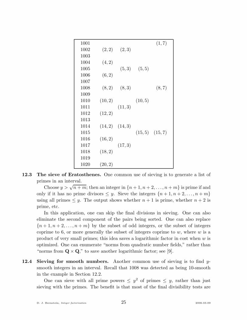
positive integers 1001, 1002, 1003, . . . , 1020. One generates the pairs (2, 2), (4, 2), . . .
for p = 2, then the pairs (2, 3), (5, 3), . . . for p = 3, then the pairs (5, 5), (10, 5), . . .
for p = 5, then the pairs (1, 7), (8, 7), . . . for p = 7. Sorting the pairs by the first
component produces
(1, 7), (2, 2), (2, 3), (4, 2), (5, 3), (5, 5), (6, 2), (8, 2), (8, 3), (8, 7), . . . ,
revealing (for example) that 1008 is divisible by 2, 3, 7. Dividing 1008 repeatedly
by 2, then 3, then 7, reveals that 1008 = 24 · 32 · 7.
D. J. Bernstein, Integer factorization 24 2006.03.09
1001 (1, 7)
1002 (2, 2) (2, 3)
1003
1004 (4, 2)
1005 (5, 3) (5, 5)
1006 (6, 2)
1007
1008 (8, 2) (8, 3) (8, 7)
1009
1010 (10, 2) (10, 5)
1011 (11, 3)
1012 (12, 2)
1013
1014 (14, 2) (14, 3)
1015 (15, 5) (15, 7)
1016 (16, 2)
1017 (17, 3)
1018 (18, 2)
1019
1020 (20, 2)
12.3 The sieve of Eratosthenes. One common use of sieving is to generate a list of
primes in an interval.
Choose y >√
n + m; then an integer in {n + 1, n + 2, . . . , n + m} is prime if and
only if it has no prime divisors ≤ y. Sieve the integers {n + 1, n + 2, . . . , n + m}using all primes ≤ y. The output shows whether n + 1 is prime, whether n + 2 is
prime, etc.
In this application, one can skip the final divisions in sieving. One can also
eliminate the second component of the pairs being sorted. One can also replace
{n + 1, n + 2, . . . , n + m} by the subset of odd integers, or the subset of integers
coprime to 6, or more generally the subset of integers coprime to w, where w is a
product of very small primes; this idea saves a logarithmic factor in cost when w is
optimized. One can enumerate “norms from quadratic number fields,” rather than
“norms from Q × Q,” to save another logarithmic factor; see [9].
12.4 Sieving for smooth numbers. Another common use of sieving is to find y-
smooth integers in an interval. Recall that 1008 was detected as being 10-smooth
in the example in Section 12.2.
One can sieve with all prime powers ≤ y2 of primes ≤ y, rather than just
sieving with the primes. The benefit is that most of the final divisibility tests are
D. J. Bernstein, Integer factorization 25 2006.03.09

eliminated: if n + i has the pair (i, p) but not (i, p2) then one does not need to try
dividing n + i by p2. The cost is small: there are only about twice as many prime
powers as primes.
One can skip all of the final divisibility tests and simply print the integers n + i
that have collected enough pairs. Imagine, for example, sorting all (i, pj, lg p), and
then adding the numbers lg p for each i: the sum of lg p is lg(n + i) if and only if
n+i is y-smooth. One can safely use low-precision approximations to the logarithms
here: the sum of lg p is below lg(n + i) − lg y if n + i is not y-smooth. An integer
n+ i divisible by a high power of a prime may be missed if one limits the exponent
j used in sieving, but this loss of effectiveness is usually outweighed by the gain in
speed.
12.5 Speed, counting bit operations. The interval n + 1, n + 2, . . . , n + m has
about m/2 multiples of 2, about m/3 multiples of 3, about m/5 multiples of 5, etc.
The total number of pairs to be sorted is about∑
p≤y(m/p) ≈ m log log y. Each
pair has lg ym bits. Sorting all the pairs takes Θ(m lg(m log log y) lg ym log log y)
bit operations; i.e., Θ(lg(m log log y) lg ym log log y) bit operations per input. One
can safely assume that m is at most yO(1)—otherwise the input integers can be
profitably partitioned—so the sorting uses Θ((lg y)2 log log y) bit operations per
input.
The initial computation of n mod p for each prime p ≤ y uses as many bit
operations as worst-case trial division, but this computation is independent of m
and becomes unnoticeable as m grows past y1+o(1).
Final divisions, to compute the unfactored part of each input, can be done in
(lg(n+m))1+o(1) bit operations per input, by techniques similar to those explained
in Section 14.3. Typically lg(n + m) ∈ (lg y)2+o(1), so sieving for large m uses a
total of (lg y)2+o(1) bit operations per input.
For comparison, recall from Section 6.4 that trial division often performs about
y/log y divisions for a single input. Trial division can finish sooner, but for typical
inputs it doesn’t. Each division uses (lg n)1+o(1) bit operations, so the total number
of bit operations per input is (y/log y)(lg n)1+o(1); i.e., y1+o(1), when y is not very
small. The rho method takes only y1/2+o(1) bit operations per input, and the
elliptic-curve method takes only exp√
(2 + o(1)) log y log log y bit operations per
input, but no known single-input method takes (lg y)O(1) bit operations per average
input.
12.6 Speed, measuring price-performance ratio. Sieving handles m inputs in only
m1+o(1) bit operations when m is large, but it also uses m1+o(1) bits of memory,
for a price-performance ratio of m2+o(1) dollar-seconds.
One can do much better with a parallel machine, as in Section 5.4. A sieving
machine costing m1+o(1) dollars can generate the m1+o(1) pairs in parallel in m0+o(1)
D. J. Bernstein, Integer factorization 26 2006.03.09
seconds, and can sort them in m0.5+o(1) seconds, for a price-performance ratio of
m1.5+o(1) dollar-seconds.
For comparison, a machine applying the elliptic-curve method to each input
separately, with m parallel elliptic-curve processors, costs m1+o(1) dollars and takes
only m0+o(1) seconds, for a price-performance ratio of m1+o(1) dollar-seconds.
From this price-performance perspective, sieving is a very bad idea when m is
large. It is useful for very small m and very small y, finding very small primes
more quickly than separate trial divisions, but the elliptic-curve method is better
at finding larger primes.
12.7 Comparing cost measures. Sections 12.5 and 12.6 used different cost mea-
sures and came to quite different conclusions about the value of sieving. Section
12.5 counted bit operations, and concluded that sieving was much better than
the elliptic-curve method for finding large primes. Section 12.6 measured price-
performance ratio, and concluded that sieving was much worse than the elliptic-
curve method for finding large primes.
The critical difference between these cost measures—at least for a sufficiently
parallelizable computation—is in the cost that they assign to long wires between
bit operations; equivalently, in the cost that they assign to instructions that access
large arrays. Measuring price-performance ratio makes each access to an array of
size m1+o(1) look as expensive as m0.5+o(1) bit operations. Counting instructions
makes each access look as inexpensive as a single bit operation.
Readers who grew up in a simple instruction-counting world might wonder
whether price-performance ratio is a useful concept. Do real computers actually
take longer to access larger arrays? The answer, in a nutshell, is yes. Counting
instructions is a useful simplification for small computers carrying out small com-
putations, but it is misleading for large computers carrying out large computations,
as the following example demonstrates.
Today’s record-setting computations are carried out on a very large, massively
parallel computer called the “Internet.” The machine has about 260 bytes of storage
spread among millions of nodes (often confusingly also called “computers”). A node
can randomly access a small array in a few nanoseconds but needs much longer to
access larger arrays. A typical node, one of the “Athlons” in my office in Chicago,
has
• 216 bytes of “L1 cache” that can stream data at about 20 nanoseconds/byte
with a latency of 22 nanoseconds;
• 218 bytes of “L2 cache” that can stream data at about 21 nanoseconds/byte
with a latency of 24 nanoseconds;
• 229 bytes of “dynamic RAM” that can stream data at about 24 nanosec-
onds/byte with a latency of 27 nanoseconds;
D. J. Bernstein, Integer factorization 27 2006.03.09
• 236 bytes of “disk” that can stream data at about 27 nanoseconds/byte with
a latency of 223 nanoseconds;
• a “local network” providing relatively slow access to 240 bytes of storage on
nearby nodes; and
• a “wide-area network” providing even slower access to the entire Internet.
Sieving is the method of choice for finding primes ≈ 210, is not easy to beat for
finding primes ≈ 220, and remains tolerable for primes ≈ 230, but is essentially
never used to find primes ≈ 240. Record-setting factorizations use sieving for small
primes and then switch to other methods, such as the elliptic-curve method, to find
larger primes.
13 Consecutive polynomial values: sieving revisited
13.1 Introduction. Sieving can be generalized from consecutive integers to consecutive
values of a low-degree polynomial. For example, one can factor positive integers
(n + 1)2 − 10, (n + 2)2 − 10, (n + 3)2 − 10, . . . , (n + m)2 − 10 by generating in
order of p, and then sorting in order of i, all pairs (i, p) such that p ≤ y is prime,
i ∈ {1, 2, . . . , m}, and p divides (n + i)2 − 10. As usual, y is a parameter chosen by
the user.
The point is that, for any particular prime p, the pairs (i, p) are a small union
of easily computed arithmetic progressions modulo p. Consider, for example, the
prime p = 997. The polynomial x2 − 10 in Fp[x] factors as (x − 134)(x − 863); so
997 divides (n + i)2 − 10 if and only if n + i mod 997 ∈ {134, 863}.
13.2 Speed. Sieving m values of an arbitrary polynomial takes almost as few bit op-
erations as sieving m consecutive integers. Factoring the polynomial modulo each
prime p ≤ y takes more work than a single division by p, but this extra work
becomes unnoticeable as m grows.
14 Arbitrary integers: exploiting fast multiplication
14.1 Introduction. Sieving finds small factors of a batch of m numbers more quickly
than finding small factors of each number separately—if the numbers are consecu-
tive integers, as in Section 12.1, or more generally consecutive values of a low-degree
polynomial, as in Section 13.1. What about numbers that don’t have such a simple
relationship?
It turns out that, by taking advantage of fast multiplication, one can find small
factors of m arbitrary integers more quickly than finding small factors of each
D. J. Bernstein, Integer factorization 28 2006.03.09
integer separately. Specifically, one can find all primes ≤ y dividing each integer in
just (lg y)O(1) bit operations, if there are at least y/(lg y)O(1) integers, each having
(lg y)O(1) bits.
This batch-factorization algorithm starts from a set P of primes and a nonempty
set S of nonzero integers to be factored. It magically figures out the set Q of primes
in P relevant to S. If #S = 1 then the algorithm is done at this point: it prints
Q, S and stops. Otherwise the algorithm splits S into two halves, say T and S −T ;
it recursively handles Q, T ; and it recursively handles Q, S − T .
How does the algorithm magically figure out which primes in P are relevant
to S? Answer: The algorithm uses a “product tree” to quickly compute a huge
number, namely the product of all the elements of S. It then uses a “remainder
tree” to quickly compute this product modulo each element of P . Computing Q is
now a simple matter of sorting: an element of P is relevant to S if and only if the
corresponding remainder is 0.
If S has y bits then the product-tree computation takes y(lg y)2+o(1) bit op-
erations; see Section 14.2. The remainder-tree computation takes y(lg y)2+o(1) bit
operations; see Section 14.3. The batch-factorization algorithm takes y(lg y)3+o(1)
bit operations; see Section 14.4. An alternate algorithm uses only y(lg y)2+o(1) bit
operations to figure out which integers are y-smooth, or more generally to compute
the y-smooth part of each integer; see Section 14.5.
I introduced the batch-factorization algorithm in [21]. The improved algorithm
for smoothness is slightly tweaked from an algorithm of Franke, Kleinjung, Morain,
and Wirth; see [22]. There are many more credits that I should be giving here—for
example, fast remainder trees were introduced in the 1970s by Fiduccia, Borodin,
and Moenck—but I’ll simply point you to the “history” parts of my paper [20].
14.2 Product trees. The “product tree of x1, x2, . . . , xm” is a tree whose root is
the product x1x2 · · ·xm; whose left subtree, for m ≥ 2, is the product tree of
x1, x2, . . . , xdm/2e; and whose right subtree, for m ≥ 2, is the product tree of
xdm/2e+1, . . . , xm−1, xm.
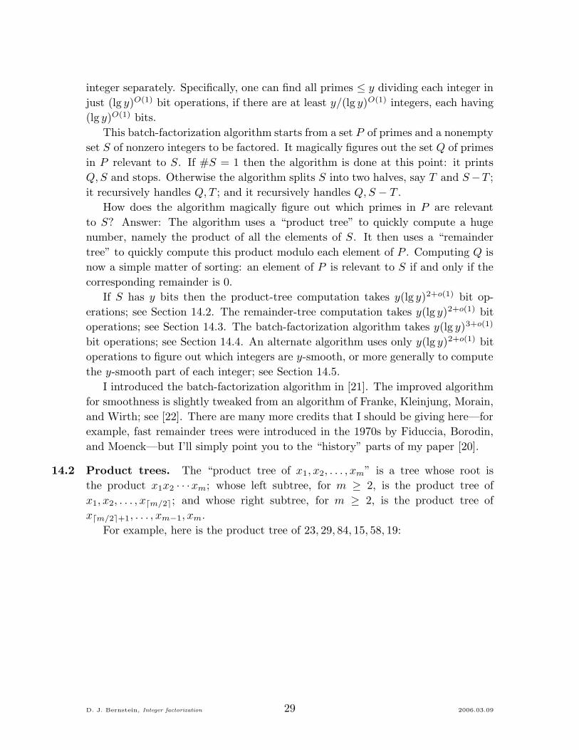
For example, here is the product tree of 23, 29, 84, 15, 58, 19:
D. J. Bernstein, Integer factorization 29 2006.03.09

926142840
56028
<<zzzzzzzz16530
hhRRRRRRRRRRRRR
667
<<zzzzzzzz84
YY222222
870
<<zzzzzzzz19
YY222222
23
EE������29
YY222222
15
EE������58
YY222222
One can compute each non-leaf node by multiplying its children. There are
approximately lg 2m levels in the tree, and the multiplications at each level use
O(b lg 2b lg lg 4b) bit operations if x1, x2, . . . , xm have b bits in total, so the product-
tree computation uses O(b lg 2m lg 2b lg lg 4b) bit operations.
A recent idea of Robert Kramer, which I call “FFT doubling,” eliminates 1/3+
o(1) of the cost of computing a product tree.
14.3 Remainder trees. The “remainder tree for Y, x1, x2, . . . , xm” has one node Y mod
X for each node X in the product tree of x1, x2, . . . , xm.
For example, here is the remainder tree of 223092870, 23, 29, 84, 15, 58, 19:
223092870
||zzzz
zzzz
((RRRRRRRRRRRRR
45402
||zzzz
zzzz
��222
222 3990
||zzzz
zzzz
��222
222
46
��������
��222
222 42 510
��������
��222
222 0
0 17 0 46
After computing the product tree, one can compute each non-root node of the
remainder tree by reducing its parent modulo the corresponding node of the prod-
uct tree. Overall the remainder-tree computation uses O(b lg 2m lg 2b lg lg 4b) bit
operations if there are b bits total in Y, x1, x2, . . . , xm.
There are several ways to save time in computing remainder trees. A “scaled
remainder tree,” described in [23], is only 3/2+o(1) times as expensive as a product
tree, if the product tree is already computed.
14.4 Speed of batch factorization. Let’s say there are b bits in the set S to be
factored. The sets Q, T, S − T that appear at the next level of recursion together
D. J. Bernstein, Integer factorization 30 2006.03.09
have at most about 2b bits. The crucial point is that the elements of Q are coprime
and divide the product of the elements of S, so the product of the elements of Q
divides the product of the elements of S, so the total length of Q is at most about
the total length of S.
The sets that appear at the next level of recursion also have at most about 2b
bits: the sets that appear in handling Q, T have at most about twice as many bits
as T , and the sets that appear in handling Q, S − T have at most about twice as
many bits as S − T .
Similar comments apply at each level of recursion. There are about lg 2m levels
of recursion, each handling a total of about 2b bits, for a total of 2b lg 2m bits.
The product-tree and remainder-tree computations use O(lg 2my lg 2b lg lg 4b) bit
operations for each bit they’re given, for a total of O(b lg 2m lg 2my lg 2b lg lg 4b) bit
operations.
There are several constant-factor improvements here. The product tree of S
can be reused for T and S − T . One can split S into more than two pieces; this is
particularly helpful when Q is noticeably smaller than S. One should also remove
extremely small primes from S in advance by a different method.
14.5 Faster smoothness detection. Define Y as the product of all primes ≤ y.
One can compute the y-smooth part of n as gcd{n, (Y mod n)2k
mod n} where
k = dlg lg ne. In particular, n is y-smooth if and only if (Y mod n)2k
mod n = 0.
Computing Y with a product tree takes y(lg y)2+o(1) bit operations. Computing
Y mod n for many integers n with a remainder tree takes y(lg y)2+o(1) bit operations
if the n’s together have approximately y bits. The final k squarings modulo n, and
the gcd, take negligible time if each n is small.
Optional extra step: If there are not very many smooth integers then finding
their prime factors, by feeding them to the batch factorization algorithm, takes
negligible extra time.
14.6 Combining methods. Recall from Sections 12.6 and 12.7 that sieving has an
unimpressive price-performance ratio as y grows—it uses a great deal of memory,
making it asymptotically more expensive than the elliptic-curve method. The same
comment applies to the batch-factorization algorithm.
Recall from Section 7 that many methods can be combined into a unified method
that’s better than any of the original methods. One could, for example, use trial
division to find primes ≤ 23; then use sieving—if the inputs are sieveable—to find
primes ≤ 215; then abort large results; then use batch factorization to find primes
≤ 228; then abort large results; then use rho to find primes ≤ 232; then abort large
results; then use p − 1, p + 1, and the elliptic-curve method to find primes ≤ 240.
Actually, I speculate that batch factorization should be used for considerably larger
primes, but I still have to finish my software for disk-based integer multiplication.
D. J. Bernstein, Integer factorization 31 2006.03.09
Finding large factors of one integer
15 The Q sieve
15.1 Introduction. The “Q sieve” tries to find a nontrivial factor of n by computing
gcd{
n,∏
i∈S i −√
∏
i∈S i(n + i)}
. Here S is a nonempty set of positive integers
such that∏
i∈S i(n+i) is a square. I’ll refer to the integer i(n+i) as a “congruence,”
alluding to the simple congruence i ≡ n + i (mod n).
To find qualifying sets S—i.e., to find square products of congruences—the Q
sieve looks at many congruences, finds some that are easily factored into primes,
and then performs linear algebra on exponent vectors modulo 2 to find a square
product of fully factored congruences.
Section 15.3 discusses the number of congruences that need to be considered
before a square product appears. Section 15.4 discusses the cost of finding fully
factored congruences. Section 15.5 discusses the cost of combining fully factored
congruences by linear algebra. The final computation of∏
i∈S i −√
∏
i∈S i(n + i)
can be done with a product tree as described in Section 14.2, or with the help of
the known factorizations of the congruences i(n + i); either way, it has negligible
cost and isn’t worth discussing further.
Sometimes the final gcd is 1 or n. In this case the Q sieve throws away one
of the i’s in S (to guarantee that S won’t be seen again), looks at some new i’s,
finds a new set S, and tries again. One can reasonably conjecture that every odd
integer n will be completely factored into prime powers by a small number of sets
S. The point is that each odd prime divisor of n has to divide∏
i −√
∏
i(n + i)
or∏
i +√
∏
i(n + i); it can’t divide both (unless it happens to divide one of the
i’s); the decision between − and + appears to be sufficiently unpredictable that
two different primes have a good chance of making different decisions.
The congruence-combination algorithms discussed in subsequent sections can be
viewed as refinements of the Q sieve, adding complications for the sake of speed.
The Q sieve was introduced by Schnorr in [125, Section 3], refining an idea of
Miller. The Q sieve was not the first congruence-combination factoring method, and
it is much slower than most of its predecessors, but it is useful as an introduction
to congruence-combination algorithms.
15.2 Example. The following tables show small factors of the integers 1, 2, 3, . . . , 20
and 612, 613, 614, . . . , 631.
D. J. Bernstein, Integer factorization 32 2006.03.09
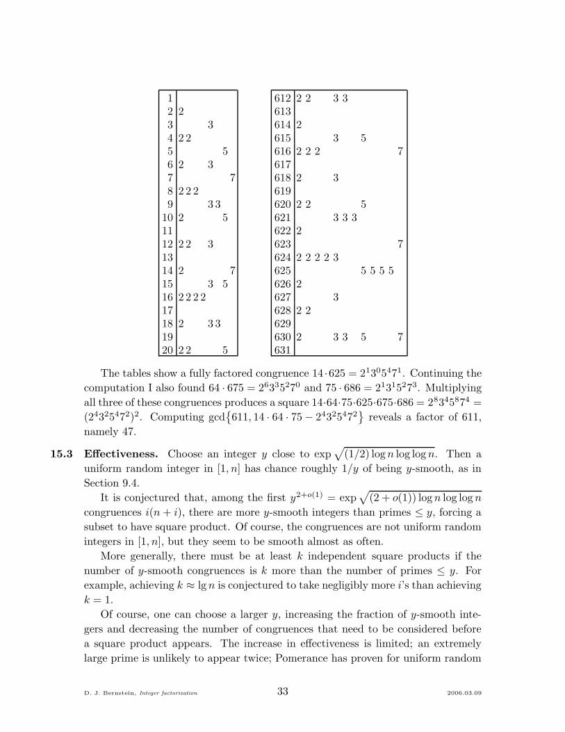
12 23 34 2 25 56 2 37 78 2 2 29 3 3
10 2 51112 2 2 31314 2 715 3 516 2 2 2 21718 2 3 31920 2 2 5
612 2 2 3 3613614 2615 3 5616 2 2 2 7617618 2 3619620 2 2 5621 3 3 3622 2623 7624 2 2 2 2 3625 5 5 5 5626 2627 3628 2 2629630 2 3 3 5 7631
The tables show a fully factored congruence 14 ·625 = 21305471. Continuing the
computation I also found 64 · 675 = 26335270 and 75 · 686 = 21315273. Multiplying
all three of these congruences produces a square 14·64·75·625·675·686 = 28345874 =
(24325472)2. Computing gcd{
611, 14 · 64 · 75 − 24325472}
reveals a factor of 611,
namely 47.
15.3 Effectiveness. Choose an integer y close to exp√
(1/2) logn log log n. Then a
uniform random integer in [1, n] has chance roughly 1/y of being y-smooth, as in
Section 9.4.
It is conjectured that, among the first y2+o(1) = exp√
(2 + o(1)) logn log log n
congruences i(n + i), there are more y-smooth integers than primes ≤ y, forcing a
subset to have square product. Of course, the congruences are not uniform random
integers in [1, n], but they seem to be smooth almost as often.
More generally, there must be at least k independent square products if the
number of y-smooth congruences is k more than the number of primes ≤ y. For
example, achieving k ≈ lg n is conjectured to take negligibly more i’s than achieving
k = 1.
Of course, one can choose a larger y, increasing the fraction of y-smooth inte-
gers and decreasing the number of congruences that need to be considered before
a square product appears. The increase in effectiveness is limited; an extremely
large prime is unlikely to appear twice; Pomerance has proven for uniform random
D. J. Bernstein, Integer factorization 33 2006.03.09
integers that one expects to look at exp√
(2 + o(1)) logn log log n integers no mat-
ter how large y is; see [118]. On the other hand, this o(1) is not the same as the
previous o(1), and experiments indicate that there is some benefit in using fairly
large primes.
15.4 Finding fully factored congruences. How do we find completely factored inte-
gers among the congruences 1(n + 1), 2(n + 2), 3(n + 3), . . .?
One answer—the answer that accounts for the word “sieve” in the name of
the Q sieve—is to choose y, sieve the integers 1, 2, 3, . . . using the primes ≤ y,
and sieve the integers n + 1, n + 2, n + 3, . . . using the primes ≤ y; see Section
12.1. If y ≈ exp√
(1/2) logn log log n then conjecturally y2+o(1) integers suffice, as
discussed in Section 15.3. Sieving y2+o(1) consecutive integers using primes ≤ y uses
y2+o(1) = exp√
(2 + o(1)) logn log log n bit operations. Actually, within y2+o(1) bit
operations, one can afford to sieve using primes ≤ y2+o(1).
See Section 15.6 for a discussion of price-performance ratio.
15.5 Combining fully factored congruences. Define the “exponent vector” of a
positive y-smooth integer 2e23e35e5 · · · as the vector (e2, e3, e5, . . .), with one entry
for each prime ≤ y.
Given the exponent vectors of some congruences, one can find a nonempty subset
with square product by finding a nonempty subset of the exponent vectors adding
up to 0 modulo 2; i.e., by finding a nonzero element of the kernel of the exponent
matrix over F2. Similarly, one can find k independent square products by finding
k independent elements of the kernel. The kernel is guaranteed to be this large if
the number of integers is k larger than the number of primes ≤ y.
Recall that sieving is conjectured to find y1+o(1) smooth congruences with
y2+o(1) bit operations if y ≈ exp√
(1/2) logn log log n. The resulting y1+o(1) ×y1+o(1) exponent matrix has y1+o(1) nonzero entries. An algorithm by Wiedemann
in [144] finds uniform random kernel elements using y2+o(1) bit operations.
One can speed up Wiedemann’s algorithm by first looking for primes p that
appear in only a few congruences: if p doesn’t appear at all then it can be removed
from the congruences; if p appears in only one congruence then it can be removed,
along with that congruence; if p appears in a few congruences then it can be removed
after those congruences are appropriately merged. The resulting algorithm still
appears to take time y2+o(1) but with a noticeably smaller o(1). There is much
more to say about linear algebra; see [119], [77], [49], [47], [84], [95], [58], and [16].
One can always save time in linear algebra by reducing y at the expense of
sieving. However, experiments suggest that linear algebra takes considerably fewer
bit operations than sieving, when y is chosen to minimize bit operations in sieving
alone.
See Section 15.6 for a discussion of price-performance ratio.
D. J. Bernstein, Integer factorization 34 2006.03.09
15.6 Price-performance ratio. Sieving has an unimpressive price-performance ratio,
taking y1.5+o(1) seconds on a parallel machine of size y1+o(1) to find y1+o(1) smooth
congruences out of y2+o(1) congruences. For comparison, the elliptic-curve method
takes only y1+o(1) seconds on a parallel machine of size y1+o(1). Record-setting
factorizations (even those labelled as “sieve” factorizations) use early aborts to
combine sieving with other methods of finding small primes.
Linear algebra has an equally unimpressive price-performance ratio: it takes
y1.5+o(1) seconds on a parallel machine of size y1+o(1). There does not seem to be
an alternative. Overall the Q sieve takes exp√
(9/8 + o(1)) logn log log n seconds
on a parallel machine of size exp√
(1/2 + o(1)) log n log log n. The machine per-
forms exp√
(2 + o(1)) logn log log n bit operations with a price-performance ratio
of exp√
(25/8 + o(1)) log n log log n dollar-seconds.
To reduce the cost of linear algebra, bringing it into balance with sieving, one can
reduce y from exp√
(1/2 + o(1)) logn log log n to exp√
(1/3 + o(1)) logn log log n.
Each congruence then has, conjecturally, chance roughly 1/y1.5 of being y-smooth.
With this revised choice of y, the Q sieve takes exp√
(3/4 + o(1)) logn log log n
seconds on a parallel machine of size exp√
(1/3 + o(1)) logn log log n, performing
exp√
(25/12 + o(1)) logn log log n bit operations with a price-performance ratio of
exp√
(25/12 + o(1)) logn log log n dollar-seconds.
15.7 Sublattices. If i is in the arithmetic progression −n + 10000032Z then i(n + i) is
divisible by 10000032. Instead of considering consecutive integers i in Z, one can
consider consecutive integers i in this arithmetic progression.
More generally, one can choose q, choose an arithmetic progression of integers
i for which the congruences i(n + i) are divisible by q, and look for fully factored
congruences within that progression. It isn’t necessary for q to be the square of a
prime, but if q is a prime above y then q needs to be incorporated into the exponent
vectors.
Varying q allows a practically unlimited supply of new congruences i(n + i)/q
on the scale of n, whereas the original congruences i(n + i) grow with i and have
only a limited supply on the scale of n. Multiple q’s won’t have much overlap if
they’re all reasonably large.
Consider, as an extreme case, taking just one i for each q, namely i = qdn/qe−n.
One hopes that the quotient i(n+i)/q = (qdn/qe−n)dn/qe is smooth. This quotient
is, on average, around n/2.
Consider, as an intermediate possibility, taking an arithmetic progression of
length y1+o(1) for each q. This allows sieving with all primes ≤ y, just like the
original Q sieve; but all of the congruences are bounded by y1+o(1)n, whereas the
original Q sieve uses congruences as large as y2+o(1)n.
An additional advantage of forcing n + i to be divisible by a large q is that it
D. J. Bernstein, Integer factorization 35 2006.03.09
helps balance the pair i, (n + i)/q. Recall from Section 6.7 that a uniform random
integer in [1, n] has chance roughly u−u of being n1/u-smooth. An integer in [1, n]
that’s a product of two independent uniform random integers in [1, n1/2] has chance
roughly (u/2)−u/2(u/2)−u/2 = u−u2u of being n1/u-smooth. The extra factor 2u is
quite noticeable.
In subsequent sections we’ll replace the polynomial i(n + i) by more subtle
choices of polynomials, producing smaller congruences; but there will always be a
limited supply of polynomial values close to the minimum. Forcing factors of q, by
considering congruences in sublattices, fixes this problem, producing a practically
unlimited supply of polynomial values close to the minimum. Often it also allows
better balancing of products.
There are many different names for minor variations of the same sublattice idea:
for example, the “special-q variation,” the “multiple-polynomial quadratic sieve,”
and the “lattice sieve.”
15.8 Finding large factors of many integers. If n′ is very close to n then there
is a large overlap between n′ + 1, n′ + 2, . . . , n′ + y2 and n + 1, n + 2, . . . , n + y2.
Consequently n and n′ can share sieving effort in the Q sieve. This idea was
introduced by Schnorr in [125, page 117].
Linear algebra might seem to become a bottleneck when this idea is applied to
many integers; but one can always reduce y to reduce the cost of linear algebra, as
in Section 15.6.
15.9 Negative integers. One can expand the Q sieve to allow i(n + i) with −n/2 <
i < 0; smaller values of i are redundant. Negative integers then require one extra
component in exponent vectors: a factorization looks like (−1)e−12e23e3 · · · , with
exponent vector (e−1, e2, e3, . . .). Similar comments apply to the algorithms in
subsequent sections.
16 The linear sieve
16.1 Introduction. The “linear sieve” tries to find a nontrivial factor of n by computing
gcd{
n,∏
(i,j)∈S(r + i)(r + j) −√
∏
(i,j)∈S(r + i)(r + j)((r + i)(r + j) − n)}
. Here
r = b√nc, and S is a nonempty set of nondecreasing pairs of positive integers such
that the product∏
(i,j)∈S(r + i)(r + j)((r + i)(r + j) − n) is a square.
In other words, the linear sieve is just like the Q sieve, except that it has a
different choice of congruences: namely, the integers (r+ i)(r+j)((r+ i)(r+j)−n),
alluding to the congruences (r + i)(r + j) ≡ (r + i)(r + j) − n (mod n).
The linear sieve allows exponent vectors (e2, e3, e5, . . . , f1, f2, . . .) representing
2e23e35e5 · · · (r +1)f1(r +2)f2 · · · . This means that a congruence is fully factored if
D. J. Bernstein, Integer factorization 36 2006.03.09
and only if the integer (r + i)(r + j)− n is fully factored. That integer is bounded
by n1/2+o(1) for reasonable ranges of i, j, whereas the Q sieve needed smoothness
of much larger integers.
Schroeppel introduced the linear sieve in 1977, along with the general idea of
congruence-combination algorithms that define congruences as consecutive values
of polynomials so that a batch of congruences can be factored by sieving.
16.2 Effectiveness. Choose an integer y close to exp√
(1/4) logn log log n. Then a
uniform random integer in [1, n1/2] has chance roughly 1/y of being y-smooth, as
in Section 15.3.
Choose z much smaller than n, and consider integers i ∈ {1, 2, 3, . . . , z}. These
integers form z(z − 1)/2 nondecreasing pairs (i, j) and thus z(z − 1)/2 congruences
(r + i)(r + j)((r + i)(r + j)−n). The integers (r + i)(r + j)−n are not much larger
than n1/2; conjecturally they have chance 1/y1+o(1) of being y-smooth, producing
z2/y1+o(1) fully factored congruences. The length of the exponent vectors is only
about z+y/log y; choosing a sufficiently large z in y1+o(1) will ensure that z2/y1+o(1)
exceeds z + y/log y.
The linear sieve is thus conjectured to find squares within the first y2+o(1) =
exp√
(1 + o(1)) log n log log n congruences.
17 The quadratic sieve
17.1 Introduction. The “quadratic sieve” tries to find a nontrivial factor of n by
computing gcd{
n,∏
i∈S(r + i) −√
∏
i∈S((r + i)2 − n)}
. Here r = b√nc, and S is
a nonempty set of positive integers such that∏
i∈S((r + i)2 − n) is a square.
The quadratic sieve can be viewed as a special case of the linear sieve, always
taking i = j; see Section 16.1. The requirement i = j makes (r + i)(r + j) a square,
meaning that the quadratic sieve doesn’t need to expand its exponent vectors in
the way that the linear sieve did. Another advantage of the quadratic sieve over
the linear sieve is that the quadratic sieve allows sublattices as in Section 15.7,
producing a practically unlimited supply of small congruences ((r + i)2 − n)/q.
The quadratic sieve was introduced by Pomerance shortly after the linear sieve.
It was used to set many factorization records. For further information see [110],
[67], [133], [53], [111], [56], [54], [130], [40], [120], [55], [136], [83], [12], [114], [137],
[131], [104], [57], [7], [10], [26], and [45]. The quadratic sieve remains one of the
most popular methods to factor integers below about 2300, although for larger sizes
it has been supplanted by the number-field sieve.
17.2 Effectiveness. The quadratic sieve, like the linear sieve, is conjectured to find
squares within the first y2+o(1) = exp√
(1 + o(1)) logn log log n congruences.
D. J. Bernstein, Integer factorization 37 2006.03.09
An interesting feature of the quadratic sieve is that only half of all primes p
are potential divisors of the congruences, namely those for which n is a square
modulo p. Integers n that are squares modulo many small primes are factored
somewhat more quickly than other integers n. Consequently one can often speed
up the quadratic sieve by replacing n with a small multiple such as 2n or 3n.
17.3 The continued-fraction method. The “continued-fraction method” produces
small squares modulo n by squaring numerators of truncations (“convergents”) of
the continued fraction for√
n. Each numerator is congruent modulo n to an integer
between −2√
n and 2√
n.
Consider, for example, n = 314159265358979323. The truncations of the con-
tinued fraction for√
n are good approximations to√
n: namely, 560499122/1,
1120998243/2, 1681497365/3, 6165490338/11, etc. The numerators of the trun-
cations have small squares modulo n: 5604991222 ≡ 403791561, 11209982432 ≡−626830243, 16814973652 ≡ 271129318, 61654903382 ≡ −465143839, etc.
The continued-fraction method is of historical interest as the first congruence-
combination factoring method. It was introduced by Lehmer and Powers in [78].
After it was refined decades later by Morrison and Brillhart in [98] it was successfully
used to factor a wide variety of integers. See [147], [110], [102], [122], [133], [148],
[146], and [143].
The quadratic sieve replaced the continued-fraction method in the early 1980s,
for reasons that seem quaint in retrospect. Subroutines at the time for linear
algebra and for smoothness detection had larger cost exponents than today’s fastest
subroutines. Pomerance in [110] conjectured that the continued-fraction method
used exp√
(1.118 . . . + o(1)) logn log log n bit operations while the quadratic sieve
used exp√
(1.020 . . . + o(1)) logn log log n bit operations. The congruences in the
quadratic sieve had a small disadvantage, namely being somewhat larger than√
n,
but they had a larger advantage, namely sieveability.
The advantage of the continued-fraction method became obsolete: sublattices
allowed the quadratic sieve to generate consistently small congruences. See Section
15.7. The advantage of the quadratic sieve also became obsolete: smoothness detec-
tion for arbitrary integers became almost as fast as sieving. See, e.g., Section 14.1.
The continued-fraction method conjecturally uses exp√
(1 + o(1)) logn log log n bit
operations when it is combined with modern subroutines for smoothness detection
and linear algebra. My impression is that the continued-fraction method is slightly
slower than the quadratic sieve, but I haven’t seen a careful analysis.
17.4 The random-squares method. One can simply consider i2 mod n for random
integers i, throwing away both sieveability and continued fractions. The resulting
algorithm has the virtue of provably factoring n into prime powers in subexponential
average time.
D. J. Bernstein, Integer factorization 38 2006.03.09

On the other hand, the congruences i2 mod n are on the scale of n rather than
n1/2, so this algorithm is much slower than the linear sieve, the quadratic sieve,
and the continued-fraction method; it’s about as slow as the Q sieve. A more
complicated idea achieves intermediate performance, with congruences on the scale
of n2/3.
If you’re interested in these provably fast “random squares” methods, see [59],
[112], and [141].
18 The number-field sieve
Not yet ready. Some references: [108], [82], [81], [4], [39], [109], [51], [24], [36], [115],
[94], [69], [18], [60], [117], [61], [62], [63], [65], [52], [64], [96], [99], [103], and [100].
Also [48] for a better exponent.
D. J. Bernstein, Integer factorization 39 2006.03.09
References
[1] — (no editor), Actes du congres international des mathematiciens, tome 3,
Gauthier-Villars Editeur, Paris, 1971. MR 54:5. See [76].
[2] — (no editor), Proceedings of the 18th annual ACM symposium on theory
of computing, Association for Computing Machinery, New York, 1986. ISBN
0–89791–193–8. See [126].
[3] — (no editor), Proceedings of the 25th annual ACM symposium on theory of
computing, Association for Computing Machinery, New York, 1983. See [6].
[4] Leonard M. Adleman, Factoring numbers using singular integers, in [11]
(1991), 64–71. Citations in this document: §18.
[5] Leonard M. Adleman, Ming-Deh Huang (editors), Algorithmic number theory:
first international symposium, ANTS-I, Ithaca, NY, USA, May 6–9, 1994,
proceedings, Lecture Notes in Computer Science, 877, Springer-Verlag, Berlin,
1994. ISBN 3–540–58691–1. MR 95j:11119. See [69].
[6] M. Ajtai, J. Komlos, E. Szemeredi, An O(n log n) sorting network, in [3]
(1983), 1–9. Citations in this document: §5.1.
[7] W. R. Alford, Carl Pomerance, Implementing the self-initializing quadratic
sieve on a distributed network, in [142] (1995), 163–174. MR 96k:11152. Ci-
tations in this document: §17.1.
[8] A. O. L. Atkin, Francois Morain, Finding suitable curves for the elliptic curve
method of factorization, Mathematics of Computation 60 (1993), 399–405.
ISSN 0025–5718. MR 93k:11115. Citations in this document: §11.1.
[9] A. O. L. Atkin, Daniel J. Bernstein, Prime sieves using binary quadratic
forms, Mathematics of Computation 73 (2004), 1023–1030. ISSN 0025–5718.
URL: http://cr.yp.to/papers.html#primesieves. Citations in this doc-
ument: §12.3.
[10] Derek Atkins, Michael Graff, Arjen K. Lenstra, Paul C. Leyland, The magic
words are squeamish ossifrage (extended abstract), in [105] (1995), 263–277.
MR 97b:94019. Citations in this document: §17.1.
[11] Baruch Awerbuch (editor), Proceedings of the 23rd annual ACM symposium
on the theory of computing, Association for Computing Machinery, New York,
1991. See [4].
[12] Eric Bach, Intractable problems in number theory, in [68] (1990), 77–93. MR
92a:11149. Citations in this document: §17.1.
[13] Eric Bach, Toward a theory of Pollard’s rho method, Information and Com-
putation 90 (1991), 139–155. ISSN 0890–5401. MR 92a:11151. Citations in
this document: §8.5.
D. J. Bernstein, Integer factorization 40 2006.03.09

[14] Eric Bach, Jeffrey Shallit, Factoring with cyclotomic polynomials, Mathe-
matics of Computation 52 (1989), 201–219. ISSN 0025–5718. MR 89k:11127.
Citations in this document: §10.6.
[15] K. E. Batcher, Sorting networks and their applications, Proceedings of the
AFIPS Spring Joint Computer Conference 32 (1968), 307–314. Citations in
this document: §5.1.
[16] Edward A. Bender, E. Rodney Canfield, An approximate probabilistic model
for structured Gaussian elimination, Journal of Algorithms 31 (1999), 271–
290. ISSN 0196–6774. MR 2000i:65064. Citations in this document: §15.5.
[17] Bruce C. Berndt, Harold G. Diamond, Adolf J. Hildebrand, Analytic num-
ber theory, volume 2, Birkhauser, Boston, 1996. ISBN 0–8176–3933–0. MR
97c:11001. See [118].
[18] Daniel J. Bernstein, The multiple-lattice number field sieve, in [19] (1995).
URL: http://cr.yp.to/papers.html. Citations in this document: §18.
[19] Daniel J. Bernstein, Detecting perfect powers in essentially linear time, and
other studies in computational number theory, Ph.D. thesis, University of
California at Berkeley, 1995. See [18].
[20] Daniel J. Bernstein, Fast multiplication and its applications, to appear in
Buhler-Stevenhagen Algorithmic number theory book. URL: http://cr.yp.
to/papers.html#multapps. ID 8758803e61822d485d54251b27b1a20d. Cita-
tions in this document: §3.1, §4.1, §4.1, §14.1.
[21] Daniel J. Bernstein, How to find small factors of integers, accepted to Math-
ematics of Computation; now being revamped. URL: http://cr.yp.to/
papers.html. Citations in this document: §14.1.
[22] Daniel J. Bernstein, How to find smooth parts of integers, draft. URL:
http://cr.yp.to/papers.html#smoothparts. ID 201a045d5bb24f43f0bd0
d97fcf5355a. Citations in this document: §14.1.
[23] Daniel J. Bernstein, Scaled remainder trees, draft. URL: http://cr.yp.to/
papers.html#scaledmod. ID e2b8da026cf72d01d97e20cf2874f278. Cita-
tions in this document: §14.3.
[24] Daniel J. Bernstein, Arjen K. Lenstra, A general number field sieve imple-
mentation, in [80] (1993), 103–126. Citations in this document: §18.
[25] Thomas Beth, Norbert Cot, Ingemar Ingemarsson (editors), Advances in
cryptology: EUROCRYPT ’84, Lecture Notes in Computer Science, 209,
Springer-Verlag, Berlin, 1985. ISBN 3–540–16076–0. MR 86m:94003. See [56],
[111].
[26] Henk Boender, Herman J. J. te Riele, Factoring integers with large-prime
variations of the quadratic sieve, Experimental Mathematics 5 (1996), 257–
273. ISSN 1058–6458. MR 97m:11155. Citations in this document: §17.1.
D. J. Bernstein, Integer factorization 41 2006.03.09
[27] Wieb Bosma, Arjen K. Lenstra, An implementation of the elliptic curve in-
teger factorization method, in [37] (1995), 119–136. MR 96d:11134. URL:
http://cr.yp.to/bib/entries.html#1995/bosma-ecm. Citations in this
document: §11.1.
[28] Richard P. Brent, Multiple-precision zero-finding methods and the com-
plexity of elementary function evaluation, in [140] (1976), 151–176.
MR 54:11843. URL: http://web.comlab.ox.ac.uk/oucl/work/richard.
brent/pub/pub028.html. Citations in this document: §4.1.
[29] Richard P. Brent, An improved Monte Carlo factorization algorithm, BIT 20
(1980), 176–184. ISSN 0006–3835. MR 82a:10017. Citations in this document:
§8.3.
[30] Richard P. Brent, Some integer factorization algorithms using elliptic curves,
Australian Computer Science Communications 8 (1986), 149–163. ISSN 0157–
3055. Citations in this document: §11.1.
[31] Richard P. Brent, Parallel algorithms for integer factorisation, in [90] (1990),
26–37. MR 91h:11148. Citations in this document: §11.1.
[32] Richard P. Brent, Factorization of the tenth Fermat number, Mathematics of
Computation 68 (1999), 429–451. ISSN 0025–5718. MR 99e:11154. Citations
in this document: §11.1, §11.1.
[33] Richard P. Brent, H. T. Kung, The area-time complexity of binary multipli-
cation, Journal of the ACM 28 (1981), 521–534. Citations in this document:
§3.4.
[34] Richard P. Brent, John M. Pollard, Factorization of the eighth Fermat num-
ber, Mathematics of Computation 36 (1981), 627–630. ISSN 0025–5718. MR
83h:10014. Citations in this document: §8.3.
[35] Ernest F. Brickell (editor), Advances in cryptology—CRYPTO ’92: 12th an-
nual international cryptology conference, Santa Barbara, California, USA,
August 16–20, 1992, proceedings, Lecture Notes in Computer Science, 740,
Springer-Verlag, Berlin, 1993. ISBN 3–540–57340–2, 0–387–57340–2. MR
95b:94001. See [104].
[36] Johannes Buchmann, J. Loho, Joerg Zayer, An implementation of the gen-
eral number field sieve (extended abstract), in [134] (1993), 159–165. MR
95e:11132. Citations in this document: §18.
[37] Wieb Bosma, Alf J. van der Poorten (editors), Computational algebra and
number theory: CANT2, Kluwer Academic Publishers, Dordrecht, 1995. ISBN
0–7923–3501–5. MR 96c:00019. See [27].
[38] Joe P. Buhler (editor), Algorithmic number theory: ANTS-III, Lecture Notes
in Computer Science, 1423, Springer-Verlag, Berlin, 1998. ISBN 3–540–
64657–4. MR 2000g:11002. See [99], [103].
D. J. Bernstein, Integer factorization 42 2006.03.09

[39] Joe P. Buhler, Hendrik W. Lenstra, Jr., Carl Pomerance, Factoring integers
with the number field sieve, in [80] (1993), 50–94. Citations in this document:
§18.
[40] T. R. Caron, Robert D. Silverman, Parallel implementation of the quadratic
sieve, Journal of Supercomputing 1 (1988), 273–290. ISSN 0920–8542. Cita-
tions in this document: §17.1.
[41] Srishti D. Chatterji (editor), Proceedings of the International Congress of
Mathematicians, Birkhauser Verlag, Basel, 1995. ISBN 3–7643–5153–5. MR
97c:00049. See [116].
[42] David Chaum (editor), Advances in cryptology: Crypto 83, Plenum Press,
New York, 1984. ISBN 0–306–41637–9. MR 86f:94001. See [53].
[43] David V. Chudnovsky, Gregory V. Chudnovsky, Harvey Cohn, Melvyn B.
Nathanson (editors), Number theory, Lecture Notes in Mathematics, 1240,
Springer-Verlag, Berlin, 1987. See [143].
[44] Henri Cohen (editor), Algorithmic number theory: second international sym-
posium, ANTS-II, Talence, France, May 18–23, 1996, proceedings, Lecture
Notes in Computer Science, 1122, Springer-Verlag, Berlin, 1996. ISBN 3–
540–61581–4. MR 97k:11001. See [58], [63].
[45] Scott P. Contini, Factoring integers with the self-initializing quadratic sieve,
M.A. thesis, University of Georgia, 1997. Citations in this document: §17.1.
[46] Stephen A. Cook, On the minimum computation time of functions, Ph.D.
thesis, Department of Mathematics, Harvard University, 1966. URL: http://
cr.yp.to/bib/entries.html#1966/cook. Citations in this document: §4.1.
[47] Don Coppersmith, Solving linear equations over GF(2): block Lanczos algo-
rithm, Linear Algebra and its Applications 192 (1993), 33–60. ISSN 0024–
3795. MR 94i:65044. Citations in this document: §15.5.
[48] Don Coppersmith, Modifications to the number field sieve, Journal of Cryp-
tology 6 (1993), 169–180. ISSN 0933–2790. MR 94h:11111. Citations in this
document: §18.
[49] Don Coppersmith, Solving homogeneous linear equations over GF(2) via block
Wiedemann algorithm, Mathematics of Computation 62 (1994), 333–350.
ISSN 0025–5718. MR 94c:11124. Citations in this document: §15.5.
[50] Don Coppersmith (editor), Advances in cryptology—CRYPTO ’95, Lecture
Notes in Computer Science, 963, Springer-Verlag, Berlin, 1995. ISBN 3–540–
60221–6. See [60].
[51] Jean-Marc Couveignes, Computing a square root for the number field sieve,
in [80] (1993), 95–102. Citations in this document: §18.
[52] James Cowie, Bruce Dodson, R.-Marije Elkenbracht-Huizing, Arjen K.
Lenstra, Peter L. Montgomery, Joerg Zayer, A World Wide number field
D. J. Bernstein, Integer factorization 43 2006.03.09

sieve factoring record: on to 512 bits, in [75] (1996), 382–394. Citations in
this document: §18.
[53] James A. Davis, Diane B. Holdridge, Factorization using the quadratic sieve
algorithm, in [42] (1984), 103–113. MR 86j:11128. Citations in this document:
§17.1.
[54] James A. Davis, Diane B. Holdridge, New results on integer factorizations,
Congressus Numerantium 46 (1985), 65–78. ISSN 0384–9864. MR 86f:11098.
Citations in this document: §17.1.
[55] James A. Davis, Diane B. Holdridge, Factorization of large integers on a
massively parallel computer, in [70] (1988), 235–243. MR 90b:11139. Citations
in this document: §17.1.
[56] James A. Davis, Diane B. Holdridge, Gustavus J. Simmons, Status report on
factoring (at the Sandia National Laboratories), in [25] (1985), 183–215. MR
87f:11105. Citations in this document: §17.1.
[57] Thomas F. Denny, Bruce Dodson, Arjen K. Lenstra, Mark S. Manasse, On the
factorization of RSA-120, in [134] (1994), 166–174. MR 95d:11170. Citations
in this document: §17.1.
[58] Thomas F. Denny, Volker Mueller, On the reduction of composed relations
from the number field sieve, in [44] (1996), 75–90. MR 98k:11184. URL:
http://cr.yp.to/bib/entries.html#1996/denny. Citations in this docu-
ment: §15.5.
[59] John D. Dixon, Asymptotically fast factorization of integers, Mathematics of
Computation 36 (1981), 255–260. ISSN 0025–5718. MR 82a:10010. Citations
in this document: §17.4.
[60] Bruce Dodson, Arjen K. Lenstra, NFS with four large primes: an explosive
experiment, in [50] (1995), 372–385. MR 98d:11156. Citations in this docu-
ment: §18.
[61] R.-Marije Elkenbracht-Huizing, Historical background of the number field
sieve factoring method, Nieuw Archief voor Wiskunde Series 4 14 (1996),
375–389. ISSN 0028–9825. MR 97i:11121. Citations in this document: §18.
[62] R.-Marije Elkenbracht-Huizing, An implementation of the number field
sieve, Experimental Mathematics 5 (1996), 231–253. ISSN 1058–6458. MR
98a:11182. Citations in this document: §18.
[63] R.-Marije Elkenbracht-Huizing, A multiple polynomial general number field
sieve, in [44] (1996), 99–114. MR 98g:11142. URL: http://cr.yp.to/bib/
entries.html#1996/elkenbracht-3. Citations in this document: §18.
[64] R.-Marije Elkenbracht-Huizing, Factoring integers with the number field sieve,
Ph.D. thesis, University of Leiden, 1997. Citations in this document: §18.
D. J. Bernstein, Integer factorization 44 2006.03.09

[65] R.-Marije Elkenbracht-Huizing, Peter L. Montgomery, Robert D. Silverman,
R. K. Wackerbarth, Samuel S. Wagstaff, Jr., The number field sieve on many
computers, in [72] (1996), 81–85. MR 2000e:11157. Citations in this document:
§18.
[66] Walter Gautschi (editor), Mathematics of Computation 1943–1993: a half-
century of computational mathematics, American Mathematical Society,
Providence, 1994. ISBN 0–8218–0291–7. MR 95j:00014. See [94], [115].
[67] Joseph L. Gerver, Factoring large numbers with a quadratic sieve, Mathe-
matics of Computation 41 (1983), 287–294. ISSN 0025–5718. MR 85c:11122.
Citations in this document: §17.1.
[68] Shafi Goldwasser (editor), Advances in cryptology—CRYPTO ’88: proceed-
ings, Lecture Notes in Computer Science, 403, Springer-Verlag, Berlin, 1990.
ISBN 3–540–97196–3, 0–387–97196–3. MR 90j:94003. See [12].
[69] Roger A. Golliver, Arjen K. Lenstra, Kevin S. McCurley, Lattice sieving and
trial division, in [5] (1994), 18–27. MR 96a:11142. URL: http://cr.yp.to/
bib/entries.html#1994/golliver. Citations in this document: §18.
[70] Christoph G. Gunther, Advances in cryptology: EUROCRYPT ’88, Lecture
Notes in Computer Science, 330, Springer-Verlag, Berlin, 1988. ISBN 3–540–
50251–3. MR 90a:94002. See [55].
[71] Louis C. Guillou, Jean-Jacques Quisquater (editors), Advances in
cryptology—EUROCRYPT ’95 (Saint-Malo, 1995), Lecture Notes in Com-
puter Science, 921, Springer-Verlag, Berlin, 1995. ISBN 3–540–59409–4. MR
96f:94001. See [95].
[72] Rajiv Gupta, Kenneth S. Williams (editors), Number theory, American Math-
ematical Society, Providence, 1999. ISBN 0–8218–0964–4. MR 99k:11005. See
[65].
[73] James L. Hafner, Kevin S. McCurley, On the distribution of running times of
certain integer factoring algorithms, Journal of Algorithms 10 (1989), 531–
556. ISSN 0196–6774. MR 91g:11157. Citations in this document: §11.5.
[74] David S. Johnson, Takao Nishizeki, Akihiro Nozaki, Herbert S. Wilf, Dis-
crete algorithms and complexity, Academic Press, Boston, 1987. ISBN 0–12–
386870–X. MR 88h:68002. See [112].
[75] Kwangjo Kim, Tsutomu Matsumoto (editors), Advances in cryptology—
ASIACRYPT ’96: international conference on the theory and applications
of cryptology and information security, Kyongju, Korea, November 3–7,
1996, proceedings, Lecture Notes in Computer Science, 1163, Springer-Verlag,
Berlin, 1996. ISBN 3–540–61872–4. MR 98g:94001. See [52].
D. J. Bernstein, Integer factorization 45 2006.03.09
[76] Donald E. Knuth, The analysis of algorithms, in [1] (1971), 269–274. MR
54:11839. URL: http://cr.yp.to/bib/entries.html#1971/knuth-gcd. Ci-
tations in this document: §4.1.
[77] Brian A. LaMacchia, Andrew M. Odlyzko, Solving large sparse linear systems
over finite fields, in [91] (1991), 109–133. Citations in this document: §15.5.
[78] Derrick H. Lehmer, R. E. Powers, On factoring large numbers, Bulletin of
the American Mathematical Society 37 (1931), 770–776. ISSN 0273–0979.
Citations in this document: §17.3.
[79] Arjen K. Lenstra, Fast and rigorous factorization under the generalized Rie-
mann hypothesis, Indagationes Mathematicae 50 (1988), 443–454. ISSN 0019–
3577. MR 90a:11152. Citations in this document: §1.7.
[80] Arjen K. Lenstra, Hendrik W. Lenstra, Jr. (editors), The development of
the number field sieve, Lecture Notes in Mathematics, 1554, Springer-Verlag,
Berlin, 1993. ISBN 3–540–57013–6. MR 96m:11116. See [24], [39], [51], [81],
[108], [109].
[81] Arjen K. Lenstra, Hendrik W. Lenstra, Jr., Mark S. Manasse, John M. Pol-
lard, The number field sieve, in [80] (1993), 11–42. Citations in this document:
§18.
[82] Arjen K. Lenstra, Hendrik W. Lenstra, Jr., Mark S. Manasse, John M. Pol-
lard, The factorization of the ninth Fermat number, Mathematics of Compu-
tation 61 (1993), 319–349. ISSN 0025–5718. MR 93k:11116. Citations in this
document: §18.
[83] Arjen K. Lenstra, Mark S. Manasse, Factoring by electronic mail, in [123]
(1990), 355–371. MR 91i:11182. Citations in this document: §17.1.
[84] Arjen K. Lenstra, Mark S. Manasse, Factoring with two large primes, Mathe-
matics of Computation 63 (1994), 785–798. ISSN 0025–5718. MR 95a:11107.
Citations in this document: §15.5.
[85] Hendrik W. Lenstra, Jr., Factoring integers with elliptic curves, Annals of
Mathematics 126 (1987), 649–673. ISSN 0003–486X. MR 89g:11125. URL:
http://links.jstor.org/sici?sici=0003-486X(198711)2:126:3<649:
FIWEC>2.0.CO;2-V. Citations in this document: §11.1, §11.5.
[86] Hendrik W. Lenstra, Jr., Jonathan Pila, Carl Pomerance, A hy-
perelliptic smoothness test, I, Philosophical Transactions of the Royal
Society of London Series A 345 (1993), 397–408. ISSN 0962–8428.
MR 94m:11107. URL: http://links.jstor.org/sici?sici=0962-8428
(19931115)345:1676<397:AHSTI>2.0.CO;2-P. Citations in this document:
§11.7.
[87] Hendrik W. Lenstra, Jr., Carl Pomerance, A rigorous time bound for fac-
toring integers, Journal of the American Mathematical Society 5 (1992),
D. J. Bernstein, Integer factorization 46 2006.03.09
483–516. ISSN 0894–0347. MR 92m:11145. URL: http://links.jstor.org/
sici?sici=0894-0347(199207)5:3<483:ARTBFF>2.0.CO;2-S. Citations in
this document: §1.7, §11.5.
[88] Hendrik W. Lenstra, Jr., Robert Tijdeman (editors), Computational methods
in number theory I, Mathematical Centre Tracts, 154, Mathematisch Cen-
trum, Amsterdam, 1982. ISBN 90–6196–248–X. MR 84c:10002. See [110].
[89] Xuemin Lin (editor), Computing theory ’98, Springer-Verlag, Singapore, 1998.
ISBN 981–3083–92–1. MR 2000g:68006. See [100].
[90] John H. Loxton (editor), Number theory and cryptography, London Mathe-
matical Society Lecture Note Series, 154, Cambridge University Press, Cam-
bridge, 1990. ISBN 0–521–39877–0. MR 90m:11003. See [31].
[91] Alfred J. Menezes, Scott A. Vanstone (editors), Advances in cryptology:
CRYPTO ’90, Lecture Notes in Computer Science, 537, Springer-Verlag,
Berlin, 1991. ISBN 3–540–54508–5. MR 94b:94002. See [77].
[92] Peter L. Montgomery, Speeding the Pollard and elliptic curve methods
of factorization, Mathematics of Computation 48 (1987), 243–264. ISSN
0025–5718. MR 88e:11130. URL: http://links.jstor.org/sici?sici=
0025-5718(198701)48:177<243:STPAEC>2.0.CO;2-3. Citations in this doc-
ument: §8.3, §11.1, §11.6.
[93] Peter L. Montgomery, An FFT extension of the elliptic curve method of fac-
torization, Ph.D. thesis, University of California at Los Angeles, 1992. URL:
http://cr.yp.to/bib/entries.html#1992/montgomery. Citations in this
document: §9.5.
[94] Peter L. Montgomery, Square roots of products of algebraic numbers, in [66]
(1994), 567–571. MR 96a:11148. Citations in this document: §18.
[95] Peter L. Montgomery, A block Lanczos algorithm for finding dependencies
over GF(2), in [71] (1995), 106–120. MR 97c:11115. Citations in this docu-
ment: §15.5.
[96] Peter L. Montgomery, Stefania Cavallar, Herman te Riele, A new world record
for the special number field sieve factoring method, CWI Quarterly 10 (1997),
105–107. ISSN 0922–5366. MR 98k:11182. Citations in this document: §18.
[97] Peter L. Montgomery, Robert D. Silverman, An FFT extension to the
P − 1 factoring algorithm, Mathematics of Computation 54 (1990), 839–
854. ISSN 0025–5718. MR 90j:11142. URL: http://cr.yp.to/bib/entries.
html#1990/montgomery. Citations in this document: §9.5.
[98] Michael A. Morrison, John Brillhart, A method of factoring and the factoriza-
tion of F7, Mathematics of Computation 29 (1975), 183–205. ISSN 0025–5718.
MR 51:8017. Citations in this document: §17.3.
D. J. Bernstein, Integer factorization 47 2006.03.09
[99] Brian Murphy, Modelling the yield of number field sieve polynomials, in [38]
(1998), 137–150. Citations in this document: §18.
[100] Brian Murphy, Richard P. Brent, On quadratic polynomials for the number
field sieve, in [89] (1998), 199–213. MR 2000i:11189. Citations in this docu-
ment: §18.
[101] Melvyn B. Nathanson (editor), Number theory, Carbondale 1979, Lecture
Notes in Mathematics, 751, Springer-Verlag, Berlin, 1979. ISBN 3–540–
09559–4. MR 81a:10004. See [147].
[102] Thorkil Naur, New integer factorizations, Mathematics of Computation 41
(1983), 687–695. ISSN 0025–5718. MR 85c:11123. Citations in this document:
§17.3.
[103] Phong Q. Nguyen, A Montgomery-like square root for the number field sieve,
in [38] (1998), 151–168. Citations in this document: §18.
[104] Rene Peralta, A quadratic sieve on the n-dimensional cube, in [35] (1993),
324–332. MR 95f:11108. Citations in this document: §17.1.
[105] Josef Pieprzyk, Reihanah Safavi-Naini (editors), Advances in cryptology—
ASIACRYPT ’94: 4th international conference on the theory and applica-
tions of cryptology, Wollongong, Australia, November 28–December 1, 1994,
proceedings, Lecture Notes in Computer Science, 917, Springer-Verlag, Berlin,
1995. ISBN 3–540–59339–X. MR 96h:94002. See [10].
[106] John M. Pollard, Theorems on factorization and primality testing, Pro-
ceedings of the Cambridge Philosophical Society 76 (1974), 521–528. ISSN
0305–0041. MR 50:6992. URL: http://cr.yp.to/bib/entries.html#1974/
pollard. Citations in this document: §8.6, §9.1.
[107] John M. Pollard, A Monte Carlo method for factorization, BIT 15 (1975),
331–334. ISSN 0006–3835. MR 52:13611. URL: http://cr.yp.to/bib/
entries.html#1975/pollard. Citations in this document: §8.1.
[108] John M. Pollard, Factoring with cubic integers, in [80] (1993), 4–10. Citations
in this document: §18.
[109] John M. Pollard, The lattice sieve, in [80] (1993), 43–49. Citations in this
document: §18.
[110] Carl Pomerance, Analysis and comparison of some integer factoring al-
gorithms, in [88] (1982), 89–139. MR 84i:10005. URL: http://cr.yp.to/
bib/entries.html#1982/pomerance. Citations in this document: §7.2, §7.3,
§17.1, §17.3, §17.3.
[111] Carl Pomerance, The quadratic sieve factoring algorithm, in [25] (1985), 169–
182. MR 87d:11098. Citations in this document: §17.1.
D. J. Bernstein, Integer factorization 48 2006.03.09
[112] Carl Pomerance, Fast, rigorous factorization and discrete logarithm algo-
rithms, in [74] (1987), 119–143. MR 88m:11109. Citations in this document:
§17.4.
[113] Carl Pomerance (editor), Cryptology and computational number theory,
American Mathematical Society, Providence, 1990. ISBN 0–8218–0155–4. MR
91k:11113. See [114].
[114] Carl Pomerance, Factoring, in [113] (1990), 27–47. MR 92b:11089. Citations
in this document: §17.1.
[115] Carl Pomerance, The number field sieve, in [66] (1994), 465–480. MR
96c:11143. Citations in this document: §18.
[116] Carl Pomerance, The role of smooth numbers in number-theoretic algorithms,
in [41] (1995), 411–422. MR 97m:11156.
[117] Carl Pomerance, A tale of two sieves, Notices of the American Mathematical
Society 43 (1996), 1473–1485. ISSN 0002–9920. MR 97f:11100. Citations in
this document: §18.
[118] Carl Pomerance, Multiplicative independence for random integers, in [17]
(1996), 703–711. MR 97k:11174. URL: http://cr.yp.to/bib/entries.
html#1996/pomerance-dep. Citations in this document: §15.3.
[119] Carl Pomerance, J. W. Smith, Reduction of huge, sparse matrices over finite
fields via created catastrophes, Experimental Mathematics 1 (1992), 89–94.
ISSN 1058–6458. Citations in this document: §15.5.
[120] Carl Pomerance, J. W. Smith, Randy Tuler, A pipeline architecture for factor-
ing large integers with the quadratic sieve algorithm, SIAM Journal on Com-
puting 17 (1988), 387–403. ISSN 0097–5397. MR 89f:11168. URL: http://
cr.yp.to/bib/entries.html#1988/pomerance. Citations in this document:
§17.1.
[121] Carl Pomerance, Jonathan Sorenson, Counting the integers factorable via cy-
clotomic methods, Journal of Algorithms 19 (1995), 250–265. ISSN 0196–
6774. MR 96e:11163. URL: http://cr.yp.to/bib/entries.html#1995/
pomerance-cyclo. Citations in this document: §9.1.
[122] Carl Pomerance, Samuel S. Wagstaff, Jr., Implementation of the continued
fraction integer factoring algorithm, Congressus Numerantium 37 (1983), 99–
118. ISSN 0384–9864. MR 85c:11124. Citations in this document: §7.2, §17.3.
[123] Jean-Jacques Quisquater, J. Vandewalle (editors), Advances in cryptology—
EUROCRYPT ’89: workshop on the theory and application of cryptographic
techniques, Houthalen, Belgium, April 10–13, 1989, proceedings, Lecture
Notes in Computer Science, 434, Springer-Verlag, Berlin, 1990. ISBN 3–540–
53433–4. MR 91h:94003. See [83].
D. J. Bernstein, Integer factorization 49 2006.03.09
[124] Manfred Schimmler, Sorting on a three dimensional cube grid, report 8604,
Christian-Albrechts-Universitat Kiel, 1986. URL: http://cr.yp.to/bib/
entries.html#1986/schimmler. Citations in this document: §5.4.
[125] Claus P. Schnorr, Refined analysis and improvements on some factoring al-
gorithms, Journal of Algorithms 3 (1982), 101–127. ISSN 0196–6774. MR
83g:10003. URL: http://cr.yp.to/bib/entries.html#1982/schnorr. Ci-
tations in this document: §1.7, §15.1, §15.8.
[126] Claus P. Schnorr, Adi Shamir, An optimal sorting algorithm for mesh-
connected computers, in [2] (1986), 255–261. Citations in this document: §5.4.
[127] Arnold Schonhage, Schnelle Berechnung von Kettenbruchentwicklugen, Acta
Informatica 1 (1971), 139–144. ISSN 0001–5903. URL: http://cr.yp.
to/bib/entries.html#1971/schoenhage-gcd. Citations in this document:
§4.1.
[128] Arnold Schonhage, Volker Strassen, Schnelle Multiplikation großer Zahlen,
Computing 7 (1971), 281–292. ISSN 0010–485X. MR 45:1431. URL:
http://cr.yp.to/bib/entries.html#1971/schoenhage-mult. Citations in
this document: §3.1.
[129] Martin Seysen, A probabilistic factorization algorithm with quadratic forms
of negative discriminant, Mathematics of Computation 48 (1987), 757–780.
ISSN 0025–5718. MR 88d:11129. URL: http://cr.yp.to/bib/entries.
html#1987/seysen. Citations in this document: §1.7.
[130] Robert D. Silverman, The multiple polynomial quadratic sieve, Mathemat-
ics of Computation 48 (1987), 329–339. ISSN 0025–5718. MR 88c:11079.
URL: http://cr.yp.to/bib/entries.html#1987/silverman. Citations in
this document: §17.1.
[131] Robert D. Silverman, Massively distributed computing and factoring large
integers, Communications of the ACM 34 (1991), 94–103. ISSN 0001–0782.
MR 92j:11152. Citations in this document: §17.1.
[132] Robert D. Silverman, Samuel S. Wagstaff, Jr., A practical analysis of the
elliptic curve factoring algorithm, Mathematics of Computation 61 (1993),
445–462. ISSN 0025–5718. MR 93k:11117. Citations in this document: §11.1.
[133] J. W. Smith, Samuel S. Wagstaff, Jr., How to crack an RSA cryptosys-
tem, Congressus Numerantium 40 (1983), 367–373. ISSN 0384–9864. MR
86d:94020. Citations in this document: §17.1, §17.3.
[134] Douglas R. Stinson (editor), Advances in cryptology—CRYPTO ’93: 13th
annual international cryptology conference, Santa Barbara, California, USA,
August 22–26, 1993, proceedings, Lecture Notes in Computer Science, 773,
Springer-Verlag, Berlin, 1994. ISBN 3–540–57766–1, 0–387–57766–1. MR
95b:94002. See [36], [57].
D. J. Bernstein, Integer factorization 50 2006.03.09

[135] Volker Strassen, Einige Resultate uber Berechnungskomplexitat, Jahresbericht
der Deutschen Mathematiker-Vereinigung 78 (1976), 1–8. MR 55:11713. Ci-
tations in this document: §8.6.
[136] Herman te Riele, Walter Lioen, Dik Winter, Factoring with the quadratic sieve
on large vector computers, Journal of Computational and Applied Mathe-
matics 27 (1989), 267–278. ISSN 0377–0427. MR 90h:11111. Citations in this
document: §17.1.
[137] Herman te Riele, Walter Lioen, Dik Winter, Factorization beyond the googol
with MPQS on a single computer, CWI Quarterly 4 (1991), 69–72. ISSN
0922–5366. MR 92i:11132. Citations in this document: §17.1.
[138] C. D. Thompson, H. T. Kung, Sorting on a mesh-connected parallel computer,
Communications of the ACM 20 (1977), 263–271. ISSN 0001–0782. Citations
in this document: §5.4.
[139] Andrei L. Toom, The complexity of a scheme of functional elements realizing
the multiplication of integers, Soviet Mathematics Doklady 3 (1963), 714–716.
ISSN 0197–6788. Citations in this document: §3.1.
[140] Joseph F. Traub, Analytic computational complexity, Academic Press, New
York, 1976. MR 52:15938. See [28].
[141] Brigitte Vallee, Generation of elements with small modular squares and
provably fast integer factoring algorithms, Mathematics of Computation 56
(1991), 823–849. ISSN 0025–5718. MR 91i:11183. Citations in this document:
§17.4.
[142] Alf J. van der Poorten, Igor Shparlinski, Horst G. Zimmer, Number-theoretic
and algebraic methods in computer science: NTAMCS ’93, World Scientific
Publishing, River Edge, 1995. ISBN 981–02–2334–X. MR 96i:11103. See [7].
[143] Samuel S. Wagstaff, Jr., J. W. Smith, Methods of factoring large integers, in
[43] (1987), 281–303. MR 88i:11098. URL: http://cr.yp.to/bib/entries.
html#1987/wagstaff. Citations in this document: §17.3.
[144] Douglas H. Wiedemann, Solving sparse linear equations over finite fields,
IEEE Transactions on Information Theory 32 (1986), 54–62. ISSN 0018–
9448. MR 87g:11166. URL: http://cr.yp.to/bib/entries.html#1986/
wiedemann. Citations in this document: §15.5.
[145] Hugh C. Williams, A p + 1 method of factoring, Mathematics of Computa-
tion 39 (1982), 225–234. ISSN 0025–5718. MR 83h:10016. Citations in this
document: §10.1.
[146] Hugh C. Williams, Marvin C. Wunderlich, On the parallel generation of the
residues for the continued fraction factoring algorithm, Mathematics of Com-
putation 48 (1987), 405–423. ISSN 0025–5718. MR 88i:11099. URL: http://
D. J. Bernstein, Integer factorization 51 2006.03.09

cr.yp.to/bib/entries.html#1987/williams. Citations in this document:
§17.3.
[147] Marvin C. Wunderlich, A running time analysis of Brillhart’s continued frac-
tion factoring method, in [101] (1979), 328–342. URL: http://cr.yp.to/
bib/entries.html#1979/wunderlich. Citations in this document: §17.3.
[148] Marvin C. Wunderlich, Implementing the continued fraction factoring algo-
rithm on parallel machines, Mathematics of Computation 44 (1985), 251–260.
ISSN 0025–5718. MR 86d:11104. Citations in this document: §17.3.
D. J. Bernstein, Integer factorization 52 2006.03.09

Index
10000 digits, finding factorization is hard, 1.2
10000 digits, proving compositeness is doable, 1.2
Artjuhov’s generalized Fermat test, see sprp test
average inputs, versus typical inputs, 1.6
average inputs, versus worst-case inputs, 1.6
Baillie-Pomerance-Selfridge-Wagstaff test, has never been observed to fail to prove
compositeness of a composite, 1.3
Baillie-Pomerance-Selfridge-Wagstaff test, proves compositeness of most
composites, 1.3
batch factorization, of arbitrary integers, introduction, 14.1
batch factorization, of consecutive integers, see sieving
batch factorization, of consecutive polynomial values, see sieving polynomial
values
batch factorization, by sieving, 12.1
batch factorization of arbitrary integers, combined with other methods, 14.6
batch factorization of arbitrary integers, speed, 14.4
batch factorization of arbitrary integers, speedups for smoothness detection, 14.5
bit operation, definition, 3.1
bit operations, division, 4.2
bit operations, greatest common divisor, 4.2
bit operations, multiplication, 3.1
bit operations, sorting, 5.1
CFRAC, see continued-fraction method
circuit, definition, 3.1
class-group method, see Schnorr-Lenstra-Shanks-Pollard-Atkin-Rickert
class-group method
class-group method, see Schnorr-Seysen-Lenstra-Lenstra-Pomerance class-group
method
continued-fraction method, definition, 17.3
correct output, versus output that has never been observed to be incorrect, 1.3
correct output, versus proven output, 1.3
cost measures, see operation count
cost measures, see parallel price-performance ratio
cost measures, see serial price-performance ratio
cyclotomic methods, summary, 10.6
division, bit operations, 4.2
division, instructions, 4.1
D. J. Bernstein, Integer factorization 53 2006.03.09
division, parallel price-performance ratio, 4.4
division, serial price-performance ratio, 4.3
early aborts, effectiveness, 7.3
early aborts, introduction, 7.1
early aborts, punctured, 7.4
early aborts, speed, 7.2
ECM, see elliptic-curve method
elliptic-curve method, algebraic structure, 11.3
elliptic-curve method, effectiveness, 11.5
elliptic-curve method, example, 11.2
elliptic-curve method, improvements, 11.6
elliptic-curve method, introduction, 11.1
elliptic-curve method, is faster at finding small prime divisors, 1.5
elliptic-curve method, speed, 11.4
exponent vector, definition, 15.5
factorization, different problems, 1.1
fast-factorials method, summary, 8.6
fast multiplication, definition, 3.1
finding all prime divisors, is a different problem from finding one prime divisor, 1.4
finding large prime divisors, is a different problem from finding small prime
divisors, 1.5
finding one factorization, is a different problem from finding one prime divisor, 1.4
finding one prime divisor, is a different problem from finding all prime divisors, 1.4
finding one prime divisor, is a different problem from finding one factorization, 1.4
finding small prime divisors, is a different problem from finding large prime
divisors, 1.5
Gauss, quote regarding factorization, 1.1
greatest common divisor, bit operations, 4.2
greatest common divisor, instructions, 4.1
greatest common divisor, parallel price-performance ratio, 4.4
greatest common divisor, serial price-performance ratio, 4.3
hyperelliptic-curve method, summary, 11.7
instructions, division, 4.1
instructions, greatest common divisor, 4.1
instructions, multiplication, 3.2
instructions, sorting, 5.2
Lenstra’s elliptic-curve method, see elliptic-curve method
linear sieve, effectiveness, 16.2
linear sieve, introduction, 16.1
multiple inputs, versus one input, 1.9
D. J. Bernstein, Integer factorization 54 2006.03.09

multiplication, bit operations, 3.1
multiplication, instructions, 3.2
multiplication, parallel price-performance ratio, 3.4
multiplication, serial price-performance ratio, 3.3
number-field sieve, conjecturally faster than class-group method, 1.7
number-field sieve, doesn’t seem to care how large the prime divisors are, 1.5
one input, versus multiple inputs, 1.9
operation count, versus parallel price-performance ratio, 1.8
operation count, versus parallel price-performance ratio, 12.7
operation count, versus serial price-performance ratio, 1.8
operation count, versus serial price-performance ratio, 12.7
output that has never been observed to be incorrect, versus correct output, 1.3
p + 1 method, effectiveness, 10.4
p + 1 method, example, 10.2
p + 1 method, improvements, 10.5
p + 1 method, introduction, 10.1
p + 1 method, speed, 10.3
p − 1 method, effectiveness, 9.4
p − 1 method, example, 9.2
p − 1 method, FFT continuation, 9.5
p − 1 method, improvements, 9.5
p − 1 method, introduction, 9.1
p − 1 method, second stage, 9.5
p − 1 method, speed, 9.3
parallel price-performance ratio, division, 4.4
parallel price-performance ratio, greatest common divisor, 4.4
parallel price-performance ratio, multiplication, 3.4
parallel price-performance ratio, sorting, 5.4
parallel price-performance ratio, versus operation count, 1.8
parallel price-performance ratio, versus operation count, 12.7
parallel price-performance ratio, versus serial price-performance ratio, 1.8
parallel price-performance ratio, versus serial price-performance ratio, 12.7
Pollard-Buhler-Lenstra-Pomerance-Adleman number-field sieve,
see number-field sieve
price-performance ratio, of parallel computations, see parallel price-performance
ratio
price-performance ratio, of serial computations, see serial price-performance ratio
prime factors, is a different problem from recognizing primes, 1.2
product tree, definition, 14.2
proven output, versus correct output, 1.3
D. J. Bernstein, Integer factorization 55 2006.03.09
punctured early aborts, see early aborts, punctured
QS, see quadratic sieve
Q sieve, combining fully factored congruences, 15.5
Q sieve, effectiveness, 15.3
Q sieve, example, 15.2
Q sieve, finding fully factored congruences, 15.4
Q sieve, introduction, 15.1
Q sieve, price-performance ratio, 15.6
Q sieve, using negative integers, 15.9
Q sieve, using sublattices, 15.7
quadratic sieve, effectiveness, 17.2
quadratic sieve, introduction, 17.1
random-squares method, definition, 17.4
recognizing primes, is a different problem from finding prime factors, 1.2
remainder tree, definition, 14.3
rho method, effectiveness, 8.5
rho method, example, 8.2
rho method, improvements, 8.3
rho method, introduction, 8.1
rho method, speed, 8.4
Schnorr-Lenstra-Shanks-Pollard-Atkin-Rickert class-group method,
has trouble factoring certain integers, 1.6
Schnorr-Seysen-Lenstra-Lenstra-Pomerance class-group method,
proven speed, 1.7
serial price-performance ratio, division, 4.3
serial price-performance ratio, greatest common divisor, 4.3
serial price-performance ratio, multiplication, 3.3
serial price-performance ratio, sorting, 5.3
serial price-performance ratio, versus operation count, 1.8
serial price-performance ratio, versus operation count, 12.7
serial price-performance ratio, versus parallel price-performance ratio, 1.8
serial price-performance ratio, versus parallel price-performance ratio, 12.7
sieve of Eratosthenes, see sieving for primes
sieving, cost, counting bit operations, 12.5
sieving, cost, counting instructions, 12.5
sieving, cost, measuring price-performance ratio, 12.6
sieving, example, 12.2
sieving, for primes, 12.3
sieving, for smooth numbers, 12.4
sieving, introduction, 12.1
D. J. Bernstein, Integer factorization 56 2006.03.09

sieving polynomial values, introduction, 13.1
sieving polynomial values, speed, 13.2
smooth, see smoothness
smoothness, definition, 6.6
smoothness, estimate, 6.7
sorting, bit operations, 5.1
sorting, instructions, 5.2
sorting, parallel price-performance ratio, 5.4
sorting, serial price-performance ratio, 5.3
SPAR, see Schnorr-Lenstra-Shanks-Pollard-Atkin-Rickert class-group method
sprp test, proves compositeness, 1.2
strong “probable”-prime test, see sprp test
trial division, definition, 6.1
trial division, effectiveness, 6.5
trial division, example, 6.2
trial division, improvements, 6.3
trial division, introduction, 6.1
trial division, speed, 6.4
typical inputs, versus average inputs, 1.6
typical inputs, versus worst-case inputs, 1.6
uniform, for circuits, definition, 3.2
uniform, for random numbers, definition, 6.7
worst-case inputs, versus average inputs, 1.6
worst-case inputs, versus typical inputs, 1.6
D. J. Bernstein, Integer factorization 57 2006.03.09
Top Related