


Languages
Pages
Legal


ISTITUTO DI POLITICA ECONOMICA
Institutions, the resource curse and the transition economies:
further evidence
Marta Spreafico
Quaderno n. 64/aprile 2013
VITA E PENSIERO
788834 3255139 >
ISBN 978-88-343-2551-3
COP Spreafico.qxd:_ 11/04/13 11:01 Page 1
Università Cattolica del Sacro Cuore
ISTITUTO DI POLITICA ECONOMICA
Institutions, the resource curse and the transition economies:
further evidence
Marta Spreafico
Quaderno n. 64/aprile 2013
VITA E PENSIERO
Marta Spreafico, Istituto di Politica Economica, Università Cattolica delSacro Cuore, Milano
I quaderni possono essere richiesti a:Istituto di Politica Economica, Università Cattolica del Sacro CuoreLargo Gemelli 1 – 20123 Milano – Tel. 02-7234.2921
www.vitaepensiero.it
All rights reserved. Photocopies for personal use of the reader, not exceeding 15% ofeach volume, may be made under the payment of a copying fee to the SIAE, inaccordance with the provisions of the law n. 633 of 22 april 1941 (art. 68, par. 4 and5). Reproductions which are not intended for personal use may be only made with thewritten permission of CLEARedi, Centro Licenze e Autorizzazioni per leRiproduzioni Editoriali, Corso di Porta Romana 108, 20122 Milano, e-mail:[email protected], web site www.clearedi.org.
Le fotocopie per uso personale del lettore possono essere effettuate nei limiti del 15%di ciascun volume dietro pagamento alla SIAE del compenso previsto dall’art. 68,commi 4 e 5, della legge 22 aprile 1941 n. 633.Le fotocopie effettuate per finalità di carattere professionale, economico ocommerciale o comunque per uso diverso da quello personale possono essereeffettuate a seguito di specifica autorizzazione rilasciata da CLEARedi, CentroLicenze e Autorizzazioni per le Riproduzioni Editoriali, Corso di Porta Romana 108, 20122 Milano, e-mail: [email protected] e sito webwww.clearedi.org
© 2013 Marta SpreaficoISBN 978-88-343-2551-3
3
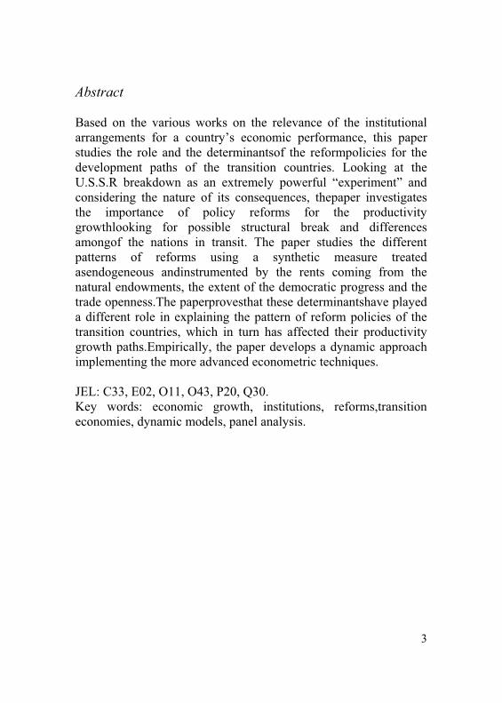
Abstract
Based on the various works on the relevance of the institutional arrangements for a country’s economic performance, this paper studies the role and the determinantsof the reformpolicies for the development paths of the transition countries. Looking at the U.S.S.R breakdown as an extremely powerful “experiment” and considering the nature of its consequences, thepaper investigates the importance of policy reforms for the productivity growthlooking for possible structural break and differences amongof the nations in transit. The paper studies the different patterns of reforms using a synthetic measure treated asendogeneous andinstrumented by the rents coming from the natural endowments, the extent of the democratic progress and the trade openness.The paperprovesthat these determinantshave played a different role in explaining the pattern of reform policies of the transition countries, which in turn has affected their productivity growth paths.Empirically, the paper develops a dynamic approach implementing the more advanced econometric techniques.
JEL: C33, E02, O11, O43, P20, Q30. Key words: economic growth, institutions, reforms,transition economies, dynamic models, panel analysis.


5
Introduction
One of the most remarkable results of the recent years of research is the positive relationship between institutions and development (North; Acemoglu, Johnson and Robinson; Hall and Jones; Rodrik; Easterly; among others). Several works have proved empirically the positive effect institutions have on the countries growth processes and the paths undertaken by the literature shows that working in a historical perspective is fruitful for several standpoints. In particular, it suggests the role of institutional arrangements could be further determined if we might observe a “structural” change of institutions and study what this has entailed for subsequent economic patterns. Transition economies are an extraordinary case of structural change of institutions. These countries lived for many years under the Communist rule, which had its own political and economic imperatives, and when these regimes were removed they had to face a new “reality” demanding new governments, new institutions and a transition to market economies. The literature1 has studied thoroughly the economic challenges of these countries focusing theoretically on the causes of the initial output collapse (among others, Blanchard and Kremer, 1997; Calvo and Coricelli, 1996; Gaddy and Ickes, 1998; Marin and Schnitzer, 1999) and empirically on the role of initial conditions and reforms strategies (liberalisation) in explaining output performance (De Melo et al. 1996, 2001; Fischer, Sahay and Vegh, 1996, 2000; Selowsky and Martin, 1997; Staehr, 2005; Lee and Jeong, 2006).Moreover, considering that the variation of the economic performance of these countries could be also determined by the new created institutional environment, the literature on transitionhas dealtwith the importance of institutions for their economic outcomes(Havrylyshyn and Van Rooden, 2003; Di Tommaso, Raiser, Weeks, 2007; Redek and Susjan, 2005, 2008;Pistor, Raiser, Gelfer, 2000; Hoff and Stiglitz, 2004).
1 For a comprehensive review, see Campos and Coricelli, 2002.
6
Institutions in these works are defined in different ways and can be either various indicators of the extent of economic freedom or measures of the democratic process and protection of property rights. Although their results confirm the existence of a positive relationship between institutional arrangements and economic performance, none of them provides the basis for a conceptual framework to analyze the impact of institutions on the economic paths of the transition countries. Exceptions are Beck and Laeven (2006) and Eicher and Schreiber (2010), who tackle this issue providing respectively a first study of the determinants of the institutional variation across theireconomies and a first attempt to capture the contemporary short term effects of a precise set of institutions via a panel methodology. Our paper, motivated by these approaches and their results, offers a novel explanation of why the so called transition economies exhibit such different stages in terms of institutional development(i.e. Estonia vs. Uzbekistan; Czech Republic vs. Moldova; Hungary vs. Turkmenistan, and so on) and provides further evidence on their importance for economic growth.Considering a specific part of the institutional environment (as Eicher and Schreiber, 2010), namely the institutions which rule the economic activity, those economic agents look at when they have to take economic decisions,we wonder about their status quo, about which forces have shaped their profile (as Beck and Laeven, 2006). Our hypothesis is that three main factors have affected the institutional development of the nations in transit. First, as communism means that everything is controlled, “commanded”, by the state, by what can be called political power, we conjecture that the countries, where the past elites remained in power, where authoritarian presidential administrations exist, where democratization process is very slow or even a “dream”, they also have known an equally slow institutional development. Second, some of the transition economiesare endowed with the presence of natural resources, whose extraction is typically controlled by state authorities. Since this clearly leads to widespread rent-seeking behaviour on the part of the government, which in turn leads to corruption - in a system
7
where bribery was already endemic – we hypothesize thatwhere there is abundance of natural resources, there is poor institutional development due to the incentives of the political elite to keep the economy “under control” in order to secure economic rents. Third, other incentives to reform the economic system are thought to come from the countries’ trade openness, from their trade relationships (Barlow, 2006). As the degree of trade openness of the transition economies, especially that of the Former Soviet Union ones, was very low,because their partners largely belonged to the Council for Mutual Economic Assistance (CMEA), we conjecture thatthe incentives coming from the trade relations with more advanced market economies have been another potential force for the institutional development.In other words, we hypothesise that theinstitutional arrangements of the countries engaged in trade relations with moreadvanced market economies are more developed. This paper shows that among the transition economies, these three dimensions have affected the evolution of the institutional arrangements, which in turn has to a certain extent affected their growth paths. Our work offers a novel approach to the explanation of the endogeneity of the institutions building in the transition countries. Moreover, we investigate whether,among these countries, the new institutional arrangements have played a different role. Focusing on the historical perspective, we decide to make a distinction between Former Soviet Union (FSU) countries and Central Eastern European (CEE) ones.In fact, the former are heritage of the Soviet Union, the latter are the so called Eastern bloc, i.e. countries that have “just” experienced Communism. The former had a common history; the latter had a soviet influence in common, which however affected them differently. Due to this, we cannot think the CEE countries lived central planning in the same radical way. Since the U.S.S.R. breakdown is a unique and extraordinary event due to its seventy years history of systematic cohesion among political system, economic policy and economic structure, we examine whether this heritage has conditioned the importance of the new institutional landscape. For this reason, the
8
analysis of the institutional determinants and the study of their impact on the economic growth is donecontrolling also for country-group. As Eicher and Schreiber, we follow the leading approach of the literature about the link between growth and institutions (Hall and Jones, 1999; Acemoglu et al., 2002, 2005) and focus only on the role of institutions to catch the economic change due to the institutional development. The rest of the paper is organized as follows. Section 2 presents our theoretical framework. Starting from the data,we also provide some empirical evidence. Section 3 presents the specification of the model, our econometric methodology and describes the variables used. Section 4 shows the estimation results. Section 5 concludes.
1. Institutions, reform policies and their determinants
In the literature, during these years of research, the word “institution” has received different names; it has been related to different part of the institutional environment. Institution mayrefer to the political system, to the economic system or, generally speaking, to all the outcomes of the normative behaviour of the government.Moreover, it happens that the same measure is associated with different labels, according to the purpose of the study.However, although researchers have studied different features of the institutional structure and called themin different ways, we all know that institutions have an unique theoretical meaning, from which we start to explain our conceptual and empirical analysis. Northtaught us that “institutions are the rules of the game of the society”. More precisely, “they define the choice set and determine transaction and production costs and, hence, the profitability and feasibility of engaging in economic activity”. At the beginning of the 1990s, the transition countries experienced the end (at least formally) of a specific set of institutions. The Communist
9
experiment ended and this automatically led to the collapse, for all of them2,of a specific typology of “economic institutions”, centralplanning. This “change” had its extreme expression for the Former Soviet Republics, which were together characterized by the same administrative decisions, management and control, where the Plans were the main instrument of strategic development. This central and hierarchical planning of the economic activity, established with the Revolution (1917) and maintained during the years of the authoritarian-dictatorial regime (until 1990), inspired the economies of the States of Eastern Europe, which in turn became Communist regimes at around the end of the World War II.Twenty years ago, the U.S.S.R. breakdown engendered a great historical change that entailed a transition from something, the past, to something else, the new realities formed, which leapt into the unknown, the market economy system.From this common background, which can be analytically conceived as exogenous, the Former Soviet Republics and the countries of the Eastern bloc needed an institutional change, new “rules of the game” for the economic activity. On this basis, we study the pattern of reform of these countries, whose outcome, the result of the reform policies implemented by each of them, is precisely what North means: that is, what economic agents see and take into account when they engage in the economic activity. Our measure of reform policies, following Eicher and Schreiber (2010)3, is a synthetic one and it is defined using the E.B.R.D. (European Bank for Reconstruction and Development) indices of assessment in nine areas: small and large-scale privatisation, governance and enterprise restructuring, price liberalisation, trade and foreign exchange system, competition policy, banking reform and interest rate liberalisation, securities market and non bank financial institutions, and infrastructure. They are concretely related to the functioning of the economic system and their values, measuring the degree of development (reform)
2 The Former Soviet Republics and the former Communist states of Eastern and Central Europe. 3 They call them “structural policies”.
10
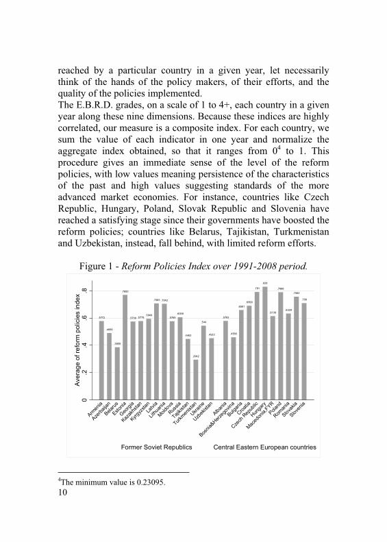
reached by a particular country in a given year, let necessarily think of the hands of the policy makers, of their efforts, and the quality of the policies implemented. The E.B.R.D. grades, on a scale of 1 to 4+, each country in a given year along these nine dimensions. Because these indices are highly correlated, our measure is a composite index. For each country, we sum the value of each indicator in one year and normalize the aggregate index obtained, so that it ranges from 04 to 1. This procedure gives an immediate sense of the level of the reform policies, with low values meaning persistence of the characteristics of the past and high values suggesting standards of the more advanced market economies. For instance, countries like Czech Republic, Hungary, Poland, Slovak Republic and Slovenia have reached a satisfying stage since their governments have boosted the reform policies; countries like Belarus, Tajikistan, Turkmenistan and Uzbekistan, instead, fall behind, with limited reform efforts.
Figure 1 - Reform Policies Index over 1991-2008 period.
4The minimum value is 0.23095.
.5772
.4896
.3859
.7692
.5739 .5778.5948
.7065 .7042
.5769.6058
.4463
.2942
.544
.4522
.5783
.4586
.6581
.6899
.791
.829
.6139
.7886
.6329
.7564
.709
0.2
.4.6
.8Av
erag
e of
refo
rm p
olic
ies
inde
x
Former Soviet Republics Central Eastern European countries
Armen
ia
Azerba
ijan
Belarus
Estonia
Georgi
a
Kazak
hstan
Kyrgyz
stanLa
tvia
Lithu
ania
Moldov
a
Russia
Tajikis
tan
Turkmen
istan
Ukraine
Uzbek
istan
Albania
Bosnia
&Herzeg
ovina
Bulgari
a
Croatia
Czech
Rep
ublic
Hunga
ry
Maced
onia,
FYR
Poland
Roman
ia
Slovak
ia
Sloven
ia
11
On the whole, the transition countries have known different reforms paths, as the reform policies have been implemented at different speeds and with different commitments.Why some transition economies have spurred reforms, while others are reform hostile? Which are the reasons behind their status-quo? And, above all, is this institutional change necessary for growth for all these countries? May its effect decrease over time? Our framework,studying the incentives of the ruling elites, features a novel account of the creation of these new institutional arrangements and provides evidence of their importance according to the group considered.We hypothesise that their key three determinants are the rents coming from the natural resources, the nature of the political system (autocracy versus democracy) and the extent of the trade openness.Natural resources. The issue of natural resources is well-studied in literature (Sachs and Warner, 1995; Sala-i-Martin, 1997; Gylfason, 2001; Auty, 2001) and it is common to refer to it in terms of “curse of natural resources”: richly endowed countries tend to have bad economic performances. In particular, the theoretical idea brought out by the literature is that the abundance of natural resources is likely to develop mechanisms which in turn lead to fall victim to the curse (Mikesell, 1997; Auty and Gelb, 2001). The natural resources phenomenon and the deterministic relationship between growth and natural resources have been studied also for the transition economies, finding evidence for the curse (Kronenberg, 2004; Esanov et al. 2001) and against it (Brunnschweiler, 2009). But what the literature does not say for the transition economies, which would be more relevant,is whether or not they have conditioned their reform policies and thus injured growth (as done for Sub-Saharan African countries by Dalmazzo and De Blasio, 2001). In other words, we wonder whether natural resources abundance has hampered the reform policies. Our hypothesis is that among transition economies the incentives of the government to reform decrease when the rents coming from natural resources increase. Reasoning in terms of the channels of transmission for the curse,
12
our insight is that the typical state control of the concessions related to the extraction of natural resources encourages corrupt and rent-seeking behaviour in the government and the political elites in order to protect theirown interests, which in turn leads to a “massive distortion” (Kronenberg, 2004) of the economic system and to a block of reform. Trade relations. The end of central planning means, at least theoretically, the simultaneous integration into the world economy and the relations with advanced market economies. Some papers have dealt with the importance of trade in transition (Kaminski, 1996; Kaminski et al., 1996) and the positive role of the trade reform policies on the economic outcome when followed by “external and internal reform” (Barlow, 2006). The openness to other countries and the commercial international relations are of great importance for the nations in transit. In fact, the centrally controlled system suppressed trade with market economies and allowed trade only between Communist countries (organized by the CMEA). In our paper, we aim at understanding whether the economic (trade) relations with advanced market economies have affected the reform processes. Sincetransition countries are likely to be diverse in terms of the nature of their trade relations, we can imagine that these commercial contacts have affected and conditioned the actions of the policy makers of these countries. More developed relations with advanced market economies require a progressive liberalization, namelyto reform the institutional arrangements implementing reform policies. It is clear that the extent of the trade openness depends on whether or not there is a direct involvement in exports and imports by ministries and state-owned trading companies. Where it does exist, there will be very few commercial relations and a low trade openness. Where there are no administrative restrictions, the degree of openness will be greater and this will lead to a general and progressive improvement of the institutional structure. If to protect their economic interests, the government dictates restrictions on the international trade, the degree of openness to the advanced market economies will be reduced and this will penalize the reform process. If the
13
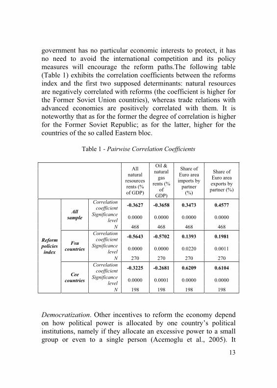
government has no particular economic interests to protect, it has no need to avoid the international competition and its policy measures will encourage the reform paths.The following table (Table 1) exhibits the correlation coefficients between the reforms index and the first two supposed determinants: natural resources are negatively correlated with reforms (the coefficient is higher for the Former Soviet Union countries), whereas trade relations with advanced economies are positively correlated with them. It is noteworthy that as for the former the degree of correlation is higher for the Former Soviet Republic; as for the latter, higher for the countries of the so called Eastern bloc.
Table 1 - Pairwise Correlation Coefficients
Allnatural
resources rents (% of GDP)
Oil & natural
gasrents (%
ofGDP)
Share of Euro area imports by
partner (%)
Share of Euro area exports by partner (%)
Allsample
Correlationcoefficient -0.3627 -0.3658 0.3473 0.4577
Significance level 0.0000 0.0000 0.0000 0.0000
N 468 468 468 468
Reform policiesindex
Fsucountries
Correlationcoefficient -0.5643 -0.5702 0.1393 0.1981
Significance level 0.0000 0.0000 0.0220 0.0011
N 270 270 270 270
Ceecountries
Correlationcoefficient -0.3225 -0.2681 0.6209 0.6104
Significance level 0.0000 0.0001 0.0000 0.0000
N 198 198 198 198
Democratization. Other incentives to reform the economy depend on how political power is allocated by one country’s political institutions, namely if they allocate an excessive power to a small group or even to a single person (Acemoglu et al., 2005). It

14
becomes clear that if political power accrues to few people, their incentives will be to act in order to protect their particular interests and not to further those of the majority of the population. The literature on transition explains in different ways that the abandonment of past institutional arrangements, that is the abandonment of the centralized control of the economy in behalf of liberalization (De Melo et al. 2001, among others), has benefited these countries, their per capita GDP. Therefore, we can gather that in those countries where political power of the elite is not threatened by any political opposition or by institutions themselves, the elite will use its power to secure economic rents and income, and will have no incentive to reform the economic environment, which would automatically reduce their rents and benefit most people. Thus, we hypothesise that among transition countries, self-interested autocratic system and authoritarian political structure are another determinant of the reform policies path. It can be noticed (Figure 2) that reforms and democratization paths tend in most cases to coincide. These three determinants are of course inevitably interrelated. The combination of non democratic institutions, which allocate political power to a small self-interested autocratic elite, with economic interests to protect (that are likely to come from both rents of natural resources and returns of state-owned dominant firms) drive the reform policies and shape the institutional development of these countries. Our analysis proves that these determinants have conditioned the reform policies of the transition countries (namely the Central Eastern European and the Former Soviet ones) and that their incremental evolution (North, 1990) has in turn affected their growth paths with some exceptions.

15
Figure 2 - The Index and the Democratization Path.
2. Econometric Analysis
Our analysis focuses on the twenty-six transition economies, over the 1991-2008 period, and examines the importance of the reform policies for the growth paths of the transition countries.Drawing on the evidence (Eicher and Schreiber, 2010) of positive relation between institutional development and economic growth, we like studying by means ofseveralregressions whether the reform policies (synthesized in the composite index explained above) have shaped differently the growth paths of the transition economies according to the twoidentified groups and whether there exists a structural breakafter the first few years following the USSR breakdown.More specifically, regarding the countries group, considering their different historical experience of centralplanning, we believe that the proper distinction is that between Central Eastern European countries and the Former Soviet Republics.Regarding the structural break, it is worth noting that the period immediately after the collapse of the Soviet Union generally
0.5
10
.51
0.5
10
.51
0.5
1
1990 1995 2000 2005 2010 1990 1995 2000 2005 2010 1990 1995 2000 2005 2010 1990 1995 2000 2005 2010
1990 1995 2000 2005 2010 1990 1995 2000 2005 2010
Armenia Azerbaijan Belarus Estonia Georgia Kazakhstan
Kyrgyzstan Latvia Lithuania Moldova Russia Tajikistan
Turkmenistan Ukraine Uzbekistan Albania Bosnia Herzegovina Bulgaria
Croatia Czech Republic Hungary Macedonia Poland Romania
Slovakia Slovenia
Reform policies index Democratization
16
saw a massive dislocation with GDP per capita collapsing, followed by a rapid recovery and then a steadier rate of growth. Hence,there may be a structural break that deserves investigation. To establish whether the “dislocation” period exists, the levels of GDP per capitawere examined and because,as expected, the first few years after the breakdown (1991-1996)seem “abnormal”, we take account of this evidence introducing a dummy in the appropriate regressions. Theoretically, talking about growth means reasoning in terms of production function, which implies to think of productivity. We employ two measures of economic performance:the GDP per person employed5, namely the gross domestic product divided by total employment in the economy, expressed in PPP terms (purchasing power parity GDP converted to 1990 constant international dollars using PPP rates) and our measure of TFP. Total Factor Productivity is defined in the usual way as
, where is output, capital, labour; is the capital share and the labour share of income (a constant equal to 0.66)6. Output is measured by GDP (constant 2000 US$)7,labour by the labour force8 and physical capital stock by the inventory equation , where is investment and the depreciation rate9. Following the literature, the initial value of capital stock is set equal to , where is the value of investment the first available year, the investment average growth rate over the estimation period10. To check the soundness and reliability of TFP measure, we regress the growth of
5 Source: World Development Indicators Database. 6 It is common in the literature to assume a constant labour share of two-thirds. 7 Source: World Development Indicators Database. 8 Labour Force, Total. Source: World Development Indicators Database. 9 As it is usual in the literature, we assume a depreciation rate of 6%. 10As the time interval between the first year with available data and the first year of the estimation period (Caselli, 2005) is less than five years, Luintel and Khan (2004) are followed and the average growth rate of investment over the estimation period is used.
17
GDP on the growth of TFP and finding a close relationship11 we use also these series to assess the growth of productivity.
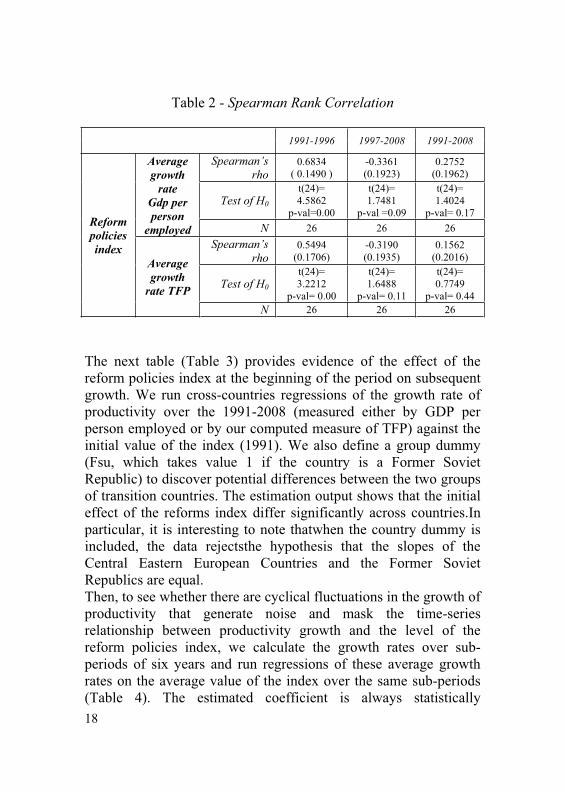
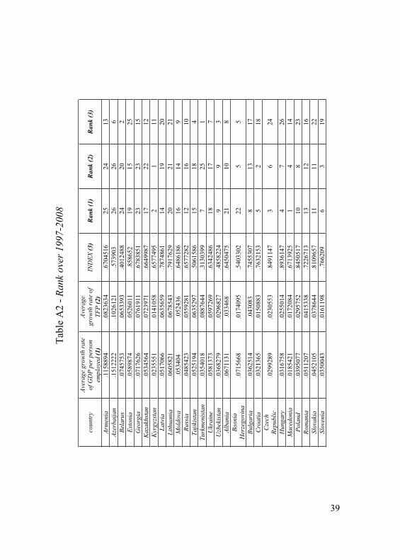
But before proceeding with the core analysis of the paper, we like exploring the impact of the reform policies on the productivity growth of these countriesfirst via a non parametric test and then via some preliminary cross-country regressions.The reform policies index is constructed by valuing the degree of structural change on a scale of 1 to 4+ and creating a composite index. In a sense, this is an ordinal measure than a cardinal one: a value of two shows greater market liberalisation than a value of one (an ordinal measure) but it is not twice as great (a cardinal measure). We treat the index as an ordinal measure and determine the strength of association between reforms and the growth paths by computing the Spearman rank correlation between the average growth rate of productivity (both measures) and the average value of the index. This is done over the whole period (1991-2008), thedislocation one (1991-1996) and the remainder of that12 (Table 2). As the results reveal, the null of independence can be rejected only for the very first years since independence, whereas after 1996 and over the whole period there seem to be no relationship between them. This suggests it is worth investigating where the relationship breaks down and whether there exists a difference between the Central Eastern European countries and the Former Soviet Republics.
11 The estimated coefficient is positive and high statistically significant (coefficient = 0.7560, standard error = 0.0316, t-statistics = 23.91) with and adjusted R-Squared of 0.5658. 12 Figures are reported in tables (Appendix A, Table A1, Table A2, Table A3).
18
Table 2 - Spearman Rank Correlation
1991-1996 1997-2008 1991-2008
Reformpolicies index
Averagegrowth
rate Gdp per person
employed
Spearman’srho
0.6834 ( 0.1490 )
-0.3361 (0.1923)
0.2752 (0.1962)
Test of H0
t(24)= 4.5862
p-val=0.00
t(24)= 1.7481
p-val =0.09
t(24)= 1.4024
p-val= 0.17 N 26 26 26
Averagegrowth
rate TFP
Spearman’srho
0.5494 (0.1706)
-0.3190 (0.1935)
0.1562 (0.2016)
Test of H0
t(24)= 3.2212
p-val= 0.00
t(24)= 1.6488
p-val= 0.11
t(24)= 0.7749
p-val= 0.44 N 26 26 26
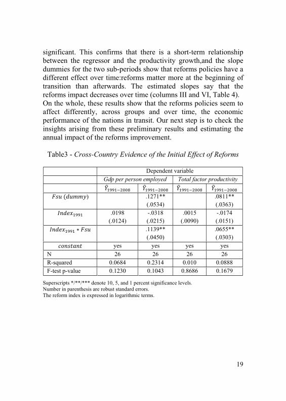
The next table (Table 3) provides evidence of the effect of the reform policies index at the beginning of the period on subsequent growth. We run cross-countries regressions of the growth rate of productivity over the 1991-2008 (measured either by GDP per person employed or by our computed measure of TFP) against the initial value of the index (1991). We also define a group dummy (Fsu, which takes value 1 if the country is a Former Soviet Republic) to discover potential differences between the two groups of transition countries. The estimation output shows that the initial effect of the reforms index differ significantly across countries.In particular, it is interesting to note thatwhen the country dummy is included, the data rejectsthe hypothesis that the slopes of the Central Eastern European Countries and the Former Soviet Republics are equal. Then, to see whether there are cyclical fluctuations in the growth of productivity that generate noise and mask the time-series relationship between productivity growth and the level of the reform policies index, we calculate the growth rates over sub-periods of six years and run regressions of these average growth rates on the average value of the index over the same sub-periods (Table 4). The estimated coefficient is always statistically
19
significant. This confirms that there is a short-term relationship between the regressor and the productivity growth,and the slope dummies for the two sub-periods show that reforms policies have a different effect over time:reforms matter more at the beginning of transition than afterwards. The estimated slopes say that the reforms impact decreases over time (columns III and VI, Table 4). On the whole, these results show that the reforms policies seem to affect differently, across groups and over time, the economic performance of the nations in transit. Our next step is to check the insights arising from these preliminary results and estimating the annual impact of the reforms improvement.
Table3 - Cross-Country Evidence of the Initial Effect of Reforms
Dependent variable Gdp per person employed Total factor productivity
) .1271** (.0534)
.0811** (.0363)
.0198 (.0124)
-.0318 (.0215)
.0015 (.0090)
-.0174 (.0151)
.1139** (.0450)
.0655** (.0303)
yes yes yes yes N 26 26 26 26 R-squared 0.0684 0.2314 0.010 0.0888 F-test p-value 0.1230 0.1043 0.8686 0.1679
Superscripts */**/*** denote 10, 5, and 1 percent significance levels. Number in parenthesis are robust standard errors. The reform index is expressed in logarithmic terms.

20
Table 4 - Long-term versus short-term relationships
Dependent variable Gdp per person employed Total factor productivity I II III IV V VI
.1033** (.0408)
.0905 (.0552)
.0220* (.0125)
.0094 (.0123)
.1205*** (.0228)
.2535*** (.0328)
.1188* (.0669)
.0978*** (.0283)
.2158*** (.0443)
.0610 (.0849)
.1924*** (.0334)
.1919*** (.0459)
.0435* (.0233)
.0353** (.0167)
yes yes yes yes yes yes N 78 78 78 78 78 78 R-squared 0.3368 0.7035 0.8180 0.2352 0.5124 0.6232 F-test p-value
0.0000 0.0000 0.0000 0.0000 0.0000 0.0000
Superscripts */**/*** denote 10, 5, and 1 percent significance levels. Number in parenthesis are robust standard errors.The dependent variables are the average growth rates of GDP per person employed and of TFP over 1991-1996 (1992 in case of TFP), 1997-2002, 2003-2008. The average values of the index are calculated over the same periods.The reform index is expressed in logarithmic terms.
2.1 Dynamic Panel Estimation
To get information about the effect of reforms policies development on economic performance, our analysis relies on panel methods. This methodology, taking into account both the cross-sectional and time variation, provides an exhaustive investigation of the ongoing incremental effect of reform policies on the countries’ economic growth. In the literature on transition, this strategy has been completely followed only by Eicher and Schreiber (2010), who are the first to analyse the growth paths of the transition countries via a dynamic specification, over the 1991-2001 period.
21
As said before, our dataset consists of the twenty-six nations in transit studied over the 1991-2008 period and since the institutional arrangements, outcome of the reform policies implemented by the governments of thesecountries, are explicitlynot recognized as exogenous in our framework, we develop formal econometric methods to deal with endogeneity. To assess the different impact of the reform policies on growth rates, according to the group of countries considered, we use the system GMM estimator (Blundell and Bond, 1998; Bond et al., 2001; Bond, 2002), whose crucial feature among others is to deliver un-biased coefficients in presence of endogenous independent variables.
Our equation model is:
(1)
where is productivity growth (exponential growth rates, both measures) in country i at time t ; is the reform policies index for the country i at time t-1, expressed in logarithmic terms, to study the impact of the policies implemented on the following growth outcome; captures country-specific effects and the time trend13.The model is first estimated considering all the transition countries and thendefining a country-group dummy (Fsu dummy) and a slope dummy variable(period b, 1997-2008) for the period following the dislocation one (1991-1996) to look for possible different impacts between the Eastern European and Former Soviet countries and over time, respectively.Then, we follow our theoretical analysis of thedeterminants of governments’ incentives to reform, based on the cross-sectionalapproach of Beck and Laeven (2006), and define ad-hoc instruments to develop in a panel setting a comprehensive explanation of the commitments to
13 Time fixed effects are not included. The rationale for that will be explained later on.
22
reform.Inspired by the hierarchy of institutions identification strategy of Eicher and Schreiber (2010), we regress our index of reform policies on the variables quantifying the rents coming from natural resources, the nature of the political institutions and the extent of the trade relations with advanced market economies. This allows to understand their particular role according to the group-specific transition path and provides the econometricfoundation to get a differently instrumented weight of the reform policies implemented. From the empirical point of view, the importance of natural resources is measured both by the total (oil, natural gas, coal, mineral and forest) natural resource rents (as percentage of GDP) and the oil and natural gas rents (as percentage of GDP) from the World Development Indicators Database.Natural resources rents are defined as the difference between the value of the natural resource production at world prices and total costs of production. These variables explicitly assessing the rents accruing to the governments are the right measure of what leads to the rent-seeking behaviour of the political elites.The nature of the political institutions is caught by the holistic polity2 variable of the Polity IV Project Database, which on a scale from -10 to +10 says the degree of democracy and autocracy, meaning -10 “full autocracy” and +10 “full democracy”. This perspective envisions a spectrum of governing authority that spans from fully institutionalized autocracies (-10 to -6), through mixed authority regimes, anocracies(-5 to +5), to fully institutionalized democracies (+6 to +10). Finally, since there is no available evidence for all the transition countries of their trade relations with the world advanced market economies, we determine their extent by the share (percentage) of imports or exports (of all products) of the euro area (12 countries) by trade partners14(from the Eurostat Statistics Database15). We know this may not exhaust their tradeconnections with all the advanced economies, but it certainly tells their links
14 The partners selected are of course the 26 nations in transit. 15 Extra-Euro area trade by partner and by SITC product group Database.
23
with the “closest” ones and gives a less imperfect and biased information than the usual degree of openness indicators.
3. Estimation Results
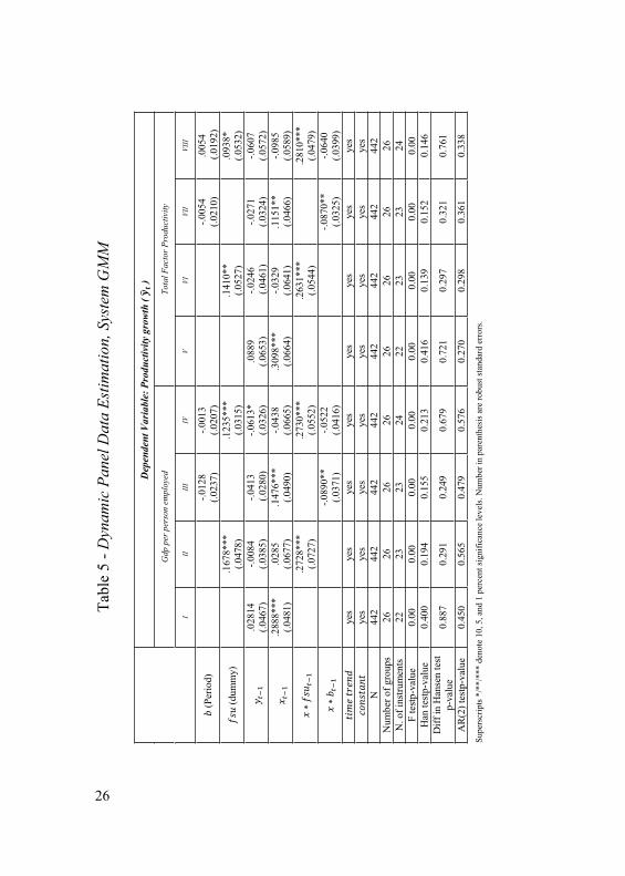
We present the main estimation results concentrating first on the impact of the reform policies impact on the productivity growth of the transition countries (equation 1), and then on the study of the reforms determinants via a two-stages approach. Table 5 presents estimation results for the equation (1) on the sample of the 26 transition countries. The annual productivity growth (the exponential growth rate of the GDP per person employed and of total factor productivity) is regressed on the lagged value of the logarithm of productivity and the lagged measure of the reform policies index, expressed in logarithmic terms. The first dynamic regression (columns I and V) proves a highly statistically significant and positive role of the reform policies for the growth paths of all the transition countries (in line with Eicher and Schreiber, 2010) and additionally it tells that the institutional arrangements, result of the policies implemented by the governments of these countries, affect the following economic outcome: a one percent increase of the reform policies index raises the growth of productivity by .28 or .30 respectively,according on the measure of productivity considered. We decide to control for the group-specific transition path (columns II and VI), studying the slope coefficient of the structural variable whenthe group dummy (Fsu) is added.The index effect is now measured as
for the Central and Eastern European Countries, but for the Former Soviet Republics. The differencebetween these values is the estimated coefficient ,which is significantly different from zero and positive.This evidence thus confirms the hypothesis that the slopes of the country-groups profiles are different,suggesting that the synthetic index change its relevancewhether we consider the Former Soviet Republics or the countries belonging to the Eastern bloc. Reform
24
policieshave a strong influence on the productivity growth of the ex Soviet Republics, whereas it plays a weak role for the productivity rates of the former Communist states of Eastern Europe. This result may reflect the different meaning of centralplanning between these two sets of countries: just the economies that lived under the Soviet system experienced the central-hierarchical administration radically. Therefore, this evidence may be theoretically explained arguing that only where central planning had its “pure” expression, the progressive abandonment of its rules has played a significant role on the economic paths. Concerning the estimation strategy, we estimate this model (equation 1) employing the system GMM16, which is recognised to be the most coherent when dealing with “ the time series dimension of the data, non-observable country specific effects, the inclusion of a lagged dependent variable among the regressors and the possibility that all explanatory variables are endogenous” (Vieira et al. 2012). As suggested by Blundell and Bond (1998) and Bond (2002), we usehigher than two lags as instruments to control for measurement error and endogeneity, and because of the reduced dimension of our sample, we create one instrument for each variable and lag distance (rather than one for each time period, variable and lag distance) in order to avoid the over-fit bias, which happens when the number of instruments is large relative to the number of observations. In fact, analyses of the issues related to the use of weak and many instruments (Roodman, 2009; Vieira et al. 2012) have revealed that instruments proliferation does not succeed inwiping out the endogenous components of the endogenous regressors, causing biased coefficients. Also the Hansen and difference-in-Hansen tests can perform poorly in the presence of many instruments, resulting in high p-values (close or equal to one), whereas the Sargan (and of course the difference-in-Sargan) cannot be weakened by their proliferation. But the problem is that the latter assumes homoschedasticity of errors for
16 One-step System GMM. This choice is due to the small dimension of the sample.
25
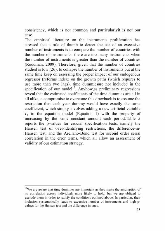
consistency, which is not common and particularlyit is not our case. The empirical literature on the instruments proliferation has stressed that a rule of thumb to detect the use of an excessive number of instruments is to compare the number of countries with the number of instruments: there are too many instruments when the number of instruments is greater than the number of countries (Roodman, 2009). Therefore, given that the number of countries studied is low (26), to collapse the number of instruments but at the same time keep on assessing the proper impact of our endogenous regressor (reforms index) on the growth paths (which requires to use more than two lags), time dummiesare not included in the specification of our model17. Anyhow,as preliminary regressions reveal that the estimated coefficients of the time dummies are all in all alike, a compromise to overcome this drawback is to assume the restriction that each year dummy would have exactly the same coefficient, which simply involves adding a new artificial variable
to the equation model (Equation 1) with the property of increasing by the same constant amount each period.Table 5 reports the p-values for crucial specification tests, namely the Hansen test of over-identifying restrictions, the difference-in-Hansen test, and the Arellano-Bond test for second order serial correlation in the error terms, which all allow an assessment of validity of our estimation strategy.
17We are aware that time dummies are important as they make the assumption of no correlation across individuals more likely to hold, but we are obliged to exclude them in order to satisfy the conditions outlined above. In particular, their inclusion systematically leads to excessive number of instruments and high p-values for the Hansen test and the difference in ones.
26
Tabl
e 5
- Dyn
amic
Pan
el D
ata
Estim
atio
n, S
yste
m G
MM
Dep
ende
nt V
aria
ble:
Pro
duct
ivity
gro
wth
( )
Gdp
per
per
son
empl
oyed
To
tal F
acto
r Pro
duct
ivity
III
III
IVV
VIVI
IVI
II
(Per
iod)
-.0
128
(.0
237)
-.0
013
(.0
207)
-.0
054
(.0
210)
.0
054
(.
0192
)
(dum
my)
.167
8***
(.0
478)
.1
235*
**
(.031
5)
.141
0**
(.0
527)
.0
938*
(.053
2)
.028
14
(.046
7)
-.008
4
(.038
5)
-.041
3
(.02
80)
-.061
3*
(.032
6)
.088
9
(.065
3)
-.024
6
(.04
61)
-.027
1
(.032
4)
-.060
7
(.0
572)
.2
888*
**
(.048
1)
.028
5
(.067
7)
.147
6***
(.0
490)
-.0
438
(.0
665)
.3
098*
**
(.066
4)
-.032
9
(.064
1)
.115
1**
(.0
466)
-.0
985
(.0
589)
.2
728*
**
(.072
7)
.273
0***
(.0
552)
.2
631*
**
(.054
4)
.281
0***
(.0
479)
-.0
890*
*
(.037
1)
-.052
2
(.041
6)
-.087
0**
(.0
325)
-.0
640
(.0
399)
ye
s ye
s ye
s ye
s ye
s ye
s ye
s ye
s ye
s ye
s ye
s ye
s ye
s ye
s ye
s ye
s N
44
2 44
2 44
2 44
2 44
2 44
2 44
2 44
2 N
umbe
r of g
roup
s 26
26
26
26
26
26
26
26
N
. of i
nstru
men
ts
22
23
23
24
22
23
23
24
F te
stp-
valu
e 0.
00
0.00
0.
00
0.00
0.
00
0.00
0.
00
0.00
H
an te
stp-
valu
e 0.
400
0.19
4 0.
155
0.21
3 0.
416
0.13
9 0.
152
0.14
6 D
iff in
Han
sen
test
p-
valu
e 0.
887
0.29
1 0.
249
0.67
9 0.
721
0.29
7 0.
321
0.76
1
AR
(2) t
estp
-val
ue
0.45
0 0.
565
0.47
9 0.
576
0.27
0 0.
298
0.36
1 0.
338
Supe
rscr
ipts
*/*
*/**
* de
note
10,
5, a
nd 1
per
cent
sign
ifica
nce
leve
ls. N
umbe
r in
pare
nthe
sis a
re ro
bust
stan
dard
err
ors.

27
Then, to explicitly test for any structural break in the model, we decide to include a dummy variable (period b) for the period following the dislocation one (1997 onwards). The regression results (Table 5, columns III and VII) show that is the estimated impact of the index during the so called dislocation period, whereas for the remainder of the series. The difference is given by that is statistically significant and negative, confirming the existence of a structural break in the model. This evidence proves that reforms matter in the very first years after the Soviet Union breakdown but then their importance becomes negligible.The last regressions (Table 5, columns IV-VIII) fully interact the core independent variable with both qualitative factors.The empirical tests reveal that there is no problem with second order autocorrelation and that the instruments are valid in all the estimated growth models, where we continue to control for the proliferation of instruments. On the whole, which lessons can be drawn from this evidence? Firstly, that the result of the reform policies implemented, namely what economic agents see and take into account when they engage in the economic activity, matter for the growth paths of the transition countries in the very first years of transition.Secondly, that it is fair to say that reforms have affected differently the transition pathsof these countries (i.e. Former Soviet Union Republics vs. Central Eastern European countries).
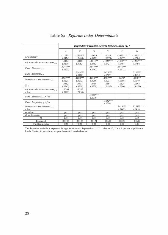
Dealing with the endogeneity of the institutional dimension, we now investigate its determinants and discover which forces drive the incentives to reform of the governments of these countries. Our strategy is to define ad-hoc instruments to give a theoretical and empirical explanation to the different commitments to reforms, which are reflected by different values of our index, according to the country considered. To get an exhaustive picture of the relative importance of the supposed determinants according to the country-group considered, we start running some preliminary regressions (Tables 6a and 6b). Then, we proceed performing a sort of two-stages approach.
28
Table 6a - Reforms Index Determinants
Dependent Variable: Reform Policies Index ( )
I II III IV V VI
(dummy) -.1123***(.0424)
-.0884** (.0408)
-.0614(.0422)
-.0315 (.0273)
-.2052***(.0437)
-.1655***(.0384)
.0404(.3139)
.0488(.3062)
-.1015**(.0402)
-.1227***(.0421)
-.1388***(.0407)
-.1264***(.0404)
.4244***(.1123)
.8547***(.1961)
.6546***(.1372)
.5543***(.1420)
.9475***(.1587)
.7552***(.1434)
.1567***(.0221)
.1600***(.0212)
.1650***(.0206)
.1787***(.0231)
.0670*(.0366)
.0740**(.0349)
.0352(.0543)
.0411(.0558)
.0458(.0578)
.0597 (.0597)
.0528(.0566)
.0563 (.0576)
-.1260(.3112)
-.1382 (.3034)
-.5984***(.1970)
-.5252***(.1719)
.1423***(.0442)
.1358***(.0416)
yes yes yes yes yes yes yes yes yes yes yes yes
N 442 442 442 442 442 442 R-squared 0.8105 0.8136 0.8171 0.8694 0.8578 0.8644
Wald test p-value 0.00 0.00 0.00 0.00 0.00 0.00
The dependent variable is expressed in logarithmic terms. Superscripts */**/*** denote 10, 5, and 1 percent significance levels. Number in parenthesis are panel corrected standard errors.

29
Table 6b - Reforms Index Determinants
Dependent Variable: Reform Policies Index ( )I II III IV V VI
(dummy) -.1162***(.0430)
-.0922**(.0413)
-.0606(.0420)
-.0655(.0430)
-.2059***(.0438)
-.1661***(.0384)
-.2384(.4304)
-.2195 (.4222)
-.1058***(.0403)
-.1014**(.0403)
-.1485***(.0410)
-.1367***(.0407)
.4208***(.1123)
.8578***(.1963)
.6533***(.1380)
.5499***(.1418)
.6941***(.1684)
.7568***(.1438)
.1557*** (.0221)
.1592***(.0212)
.1644***(.0205)
.1648***(.0206)
.0666*(.0365)
.0738**(.0349)
.0338(.0544)
.0398 (.0560)
.0466 (.0578)
.0463 (.0576)
.0539(.0565)
.0576(.0575)
.1499(.4216)
.1269(.4135)
-.6025***(.1971)
-.3155(.1946)
.1428***(.0444)
.1366***(.0419)
yes yes yes yes yes yes yes yes yes yes yes yes
N 442 442 442 442 442 442 R-squared 0.8107 0.8139 0.8177 0.8165 0.8616 0.8676
Wald test p-value 0.00 0.00 0.00 0.00 0.00 0.00
The dependent variable is expressed in logarithmic terms. Superscripts */**/*** denote 10, 5, and 1 percent significance levels. Number in parenthesis are panel corrected standard errors.
The econometric outputs confirm that the hypothesized determinants have shaped the reforms paths of these countries: they are lagged as it isthe past combination of political institutions with economic interests that drives the incentives to reform of the policy makers. In particular, allowing their slopes to differ (we interact each of them with the FSU dummy), we can understand whether they have a different importance depending onthe country group considered. Concerning natural resources (when both all natural resources and just oil and gas are taken into account), as the coefficients of the interaction term and the single variable (Table 6a and 6b, first and second columns) are not statistically significant,we do not have evidence against the hypothesis that one slope over groups of countries suffices to express the effect of natural resources on the reforms index. Concerning trade openness and democratic institutions, instead,the proxies coefficients reveal

30
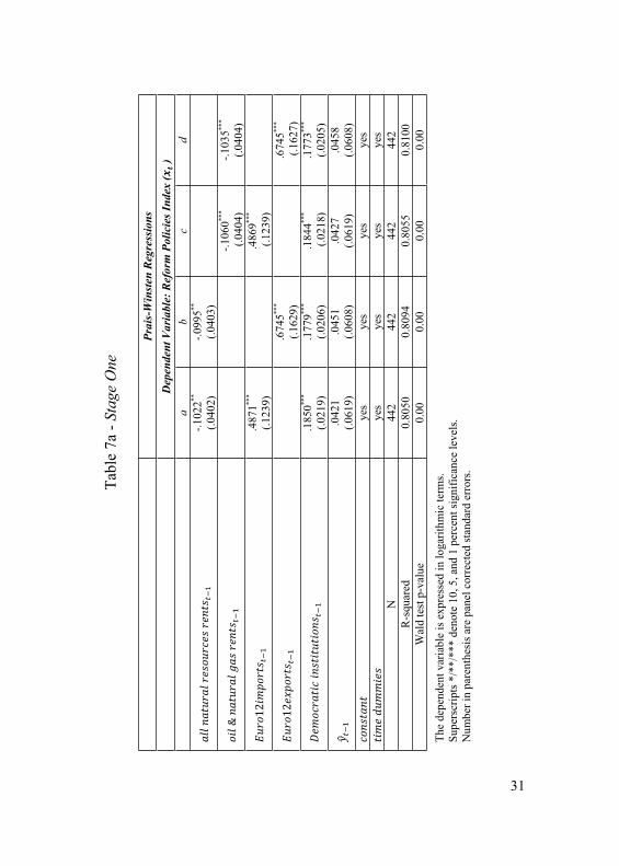
that relations with advanced market economies play a major role for the Central and Eastern European countries, whereas democratization has a greater effect among the Former Soviet Republics.Discovered the relative effects of these forces for the reforms paths of these countries, we continue our study and develop a panel identification strategy that employs these new instruments18. At the first stage, we regress our reform policies index (expressed in logarithmic terms)on the lagged values of the rents coming from all the natural resources (and alternatively just from oil and natural gas), the nature of the political institutions, and the extent of the trade relations with advanced market economies (either the percentage of imports or the percentage of exports of the twelve core countries of the Euro area by trade partner). As preliminary tests reveal that heteroschedasticity,cross-sectional correlation and within panel AR(1) autocorrelation are important issues, we calculate panel-corrected standard error estimates of our linear cross-sectional time-series model. Then, at the second stage, we provide System-GMM estimates of thereforms index using the fitted series stemming from the first stage regression. In particular, the two stages approach is implemented taking into consideration the whole sample and then (as before)studying the impact of the reforms policies depending on the country-group and the stage of transition.
18 It is of course fundamental that these instruments influence economic development only via reforms policies. When specified as independent variables in Sys-GMM regressions, it seems they do not affect productivity growth significantly (Appendix B, Table B1).
31
Tabl
e 7a
- St
age
One
Prai
s-W
inst
en R
egre
ssio
nsD
epen
dent
Var
iabl
e: R
efor
m P
olic
ies I
ndex
( )
ab
cd
-.102
2**
(.040
2)
-.099
5**
(.040
3)
-.106
0***
(.04
04)
-.103
5***
(.040
4)
.487
1***
(.123
9)
.486
9***
(.12
39)
.674
5***
(.162
9)
.674
5***
(.16
27)
.185
0***
(.021
9)
.177
9***
(.020
6)
.184
4***
(.02
18)
.177
3***
(.020
5)
.042
1
(.061
9)
.045
1
(.0
608)
.0
427
(.0
619)
.0
458
(.0
608)
ye
s ye
s ye
s ye
s ye
s ye
s ye
s ye
s N
44
2 44
2 44
2 44
2 R
-squ
ared
0.
8050
0.
8094
0.
8055
0.
8100
W
ald
test
p-v
alue
0.
00
0.00
0.
00
0.00
The
depe
nden
t var
iabl
e is
exp
ress
ed in
loga
rithm
ic te
rms.
Supe
rscr
ipts
*/*
*/**
* de
note
10,
5, a
nd 1
per
cent
sign
ifica
nce
leve
ls.
Num
ber i
n pa
rent
hesi
s are
pan
el c
orre
cted
stan
dard
err
ors.
32
Tabl
e 7b
- St
age
Two
Dep
ende
nt V
aria
ble:
Pro
duct
ivity
gro
wth
( )
Gdp
per
per
son
empl
oyed
To
tal F
acto
r Pro
duct
ivity
IaIIb
IIIc
IVd
VaVI
bVI
IcVI
IId
.061
2
(.048
1)
.052
7
(.045
6481
) .0
598
(.0
479)
.0
514
(.0
454)
.0
008
(.0
256)
-.0
088
(.0
242)
.0
004
(.0
256)
-.0
092
(.0
242)
.2
561*
**
(.0
734)
.2
430*
**
(.072
4)
.254
9***
(.0
733)
.2
420*
**
(.072
3)
.172
4***
(.0
432)
.1
614*
**
(.042
9)
.171
9***
(.0
433)
.1
609*
**
(.043
1)
yes
yes
yes
yes
yes
yes
yes
yes
yes
yes
yes
yes
yes
yes
yes
yes
N
416
416
416
416
416
416
416
416
Num
ber o
f gr
oups
26
26
26
26
26
26
26
26
Num
ber o
f in
stru
men
ts
22
22
22
22
22
22
22
22
F te
st p
-val
ue
0.00
0.
00
0.00
0.
00
0.00
0.
00
0.00
0.
00
Han
sen
test
p-
valu
e 0.
250
0.22
8 0.
241
0.22
2 0.
169
0.20
3 0.
170
0.20
4
Diff
in H
anse
n te
stp-
valu
e 0.
716
0.69
0 0.
672
0.66
7 0.
341
0.53
9 0.
346
0.54
0
AR
(2) t
est
p-va
lue
0.69
3 0.
714
0.69
2 0.
713
0.14
2 0.
152
0.14
2 0.
151
Supe
rscr
ipts
*/*
*/**
* de
note
10,
5, a
nd 1
per
cent
sign
ifica
nce
leve
ls.
Num
ber i
n pa
rent
hesi
s are
robu
st st
anda
rd e
rror
s.

33
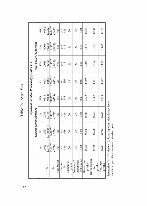
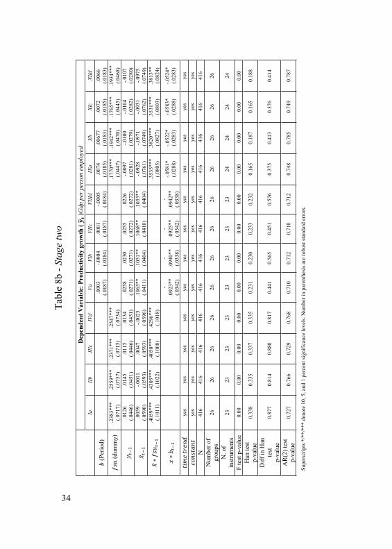
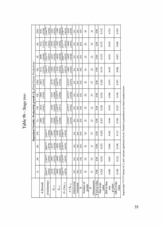
Tables 7a and 7b show the regressions results of our dynamic instrumented approach. In particular, the former exhibits that all the forces conjectured to have driven the reform paths of these countries are statistically significant. We see that the rents accrued at time t-1, both those coming from all natural resources and those coming just from oil and natural gas, have affected negatively the reform policies index; that the earlier extent of trade relations with the Euro area (measured either in terms of imports or in terms of exports) has encouraged the reform paths; and that the evolution of the political institutions toward a democratic allocation of political power has benefited the economic environment. The goodness of fit of the regressions (Table 7a) is considerable, as the three core determinants are highly statistically significant. The other table (Table 7b) exhibits the second-stage regressions, where the reform policies index is the fitted series that comes from the correspondent column of the first-stage output. We can notice that the results are consistent with an estimated coefficient positive and statistically significant at one percent level.Then, we check whether the evidence about the structural break and the existence of a different impact of reforms, according to the countries group considered, is confirmed implementing this “instrumented” system GMM estimator (Table 8b and 9b).The econometric output of Table 8b displays the second-stage estimated regressions depending on the instruments considered (columns abcand d of Table 7a), when productivity is measured by Gdp per person employed; Table 9b, when it is measured by TFP.
34
Tabl
e 8b
- St
age
two
Dep
ende
nt V
aria
ble:
Pro
duct
ivity
gro
wth
( )G
dp p
er p
erso
n em
ploy
edIa
IIbIII
cIV
dVa
VIb
VIIc
VIIId
IXa
Xb
XIc
XIId
(Per
iod)
.000
3(.0
187)
-.0
004
(.018
4)
.000
1(.0
187)
-.0
005
(.018
4)
.007
4(.0
185)
.0
0677
(.018
3)
.007
2(.0
185)
.0
066
(.018
3)
(dum
my)
.2
383*
**(.0
717)
.2
559*
**(.0
737)
.2
371*
**(.0
715)
.2
547*
**(.0
734)
.1
770*
**(.0
447)
.1
942*
**(.0
470)
.1
765*
**(.0
445)
.1
934*
**(.0
468)
.0
126
(.044
6)
.014
5(.0
451)
.0
115
(.044
6)
.013
4(.0
451)
.0
258
(.027
1)
.023
0(.0
271)
.0
255
(.027
2)
.022
6(.0
272)
-.0
097
(.028
1)
-.010
0(.0
279)
-.0
104
(.028
2)
-.010
7(.0
280)
.0
059
(.059
0)
-.001
1(.0
593)
.0
047
(.059
3)
-.002
3(.0
596)
.1
065*
*(.0
411)
.1
051*
*(.0
404)
.1
068*
*(.0
410)
.1
055*
*(.0
404)
-.0
928
(.076
1)
-.097
1(.0
749)
-.0
931
(.076
2)
-.097
5(.0
749)
.4
059*
**(.1
011)
.4
305*
**(.1
022)
.4
050*
**(.1
008)
.4
296*
**(.1
018)
.3
535*
**(.0
805)
.3
820*
**(.0
827)
.3
531*
**(.0
803)
.3
813*
*(.0
824)
-.0
923*
*(.0
342)
-.0
940*
*(.0
338)
-.0
925*
*(.0
342)
-.0
942*
*(.0
338)
-.058
1*(.0
288)
-.0
522*
(.028
3)
-.058
3*(.0
288)
-.0
524*
(.028
3)
yes
yes
yes
yes
yes
yes
yes
yes
yes
yes
yes
yes
yes
yes
yes
yes
yes
yes
yes
yes
yes
yes
yes
yes
N41
6 41
6 41
6 41
6 41
6 41
6 41
6 41
6 41
6 41
6 41
6 41
6 N
umbe
r of
grou
ps
26
26
26
26
26
26
26
26
26
26
26
26
N. o
f in
stru
men
ts
23
23
23
23
23
23
23
23
24
24
24
24
F te
st p
-val
ue
0.00
0.
00
0.00
0.
00
0.00
0.
00
0.00
0.
00
0.00
0.
00
0.00
0.
00
Han
test
p-
valu
e 0.
338
0.33
5 0.
337
0.33
5 0.
231
0.23
0 0.
233
0.23
2 0.
165
0.18
7 0.
165
0.18
8
Diff
in H
an
test
p-
valu
e 0.
877
0.81
4 0.
880
0.81
7 0.
441
0.56
5 0.
451
0.57
6 0.
375
0.41
3 0.
376
0.41
4
AR
(2) t
est
p-va
lue
0.72
7 0.
766
0.72
9 0.
768
0.71
0 0.
712
0.71
0 0.
712
0.74
8 0.
785
0.74
9 0.
787
Supe
rscr
ipts
*/*
*/**
* de
note
10,
5, a
nd 1
per
cent
sign
ifica
nce
leve
ls. N
umbe
r in
pare
nthe
sis a
re ro
bust
stan
dard
err
ors.
35
Tabl
e 9b
- St
age
two
Dep
ende
nt V
aria
ble:
Pro
duct
ivity
gro
wth
( )T
otal
Fac
tor P
rodu
ctiv
ityIa
IIbIII
cIV
dVa
VIb
VIIc
VIIId
IXa
Xb
XIc
XIId
(Per
iod)
-.0
003
(.018
2)
-.001
4(.0
181)
-.0
004
(.018
2)
-.001
5(.0
181)
.0
113
(.019
7)
.009
0(.0
188)
.0
113
(.019
7)
.010
1(.0
198)
(dum
my)
.2
016*
**(.0
582)
.2
196*
**(.0
593)
.2
005*
**(.0
578)
.2
185*
**(.0
590)
.1
386*
**(.0
363)
.1
501*
**(.0
327)
.1
378
(.036
2)
.154
4***
(.036
9)
-.012
8(.0
335)
-.0
091
(.033
5)
-.013
5(.0
334)
-.0
097
(.033
4)
-.016
8(.0
200)
-.0
180
(.019
5)
-.016
7(.0
200)
-.0
179
(.019
5)
-.043
6(.0
293)
-.0
221
(.032
6)
-.043
9(.0
293)
-.0
421
(.029
1)
-.004
9(.0
444)
-.0
099
(.043
2)
-.005
8(.0
447)
-.0
109
(.043
5)
.115
8***
(.030
9)
.116
8***
(.031
7)
.115
9***
(.030
8)
.116
8***
(.031
6)
-.101
8(.0
654)
-.0
624
(.052
0)
-.102
5(.0
654)
-.1
009
(.064
3)
.358
6***
(.067
9)
.379
5***
(.067
9)
.357
9***
(.067
8)
.378
8***
(.067
8)
.336
2***
(.061
5)
.308
8***
(.062
5)
.335
7***
(.061
5)
.359
0***
(.061
4)
-.072
9**
(.033
0)
-.075
3**
(.032
6)
-.073
2**
(.033
0)
-.075
5**
(.032
7)
-.046
5(.0
302)
-.0
459
(.034
8)
-.046
8(.0
303)
-.0
420
(.029
9)
yes
yes
yes
yes
yes
yes
yes
yes
yes
yes
yes
yes
yes
yes
yes
yes
yes
yes
yes
yes
yes
yes
yes
yes
N41
6 41
6 41
6 41
6 41
6 41
6 41
6 41
6 41
6 41
6 41
6 41
6 N
umbe
r of
grou
ps
26
26
26
26
26
26
26
26
26
26
26
26
N.
ofin
stru
men
ts
23
23
23
23
23
23
23
23
24
24
24
24
F te
st p
-val
ue
0.00
0.
00
0.00
0.
00
0.00
0.
00
0.00
0.
00
0.00
0.
00
0.00
0.
00
Han
test
p-va
lue
0.22
4 0.
222
0.22
2 0.
220
0.22
7 0.
220
0.22
6 0.
220
0.17
4 0.
153
0.17
2 0.
172
Diff
in H
an
test
p-
valu
e 0.
889
0.89
7 0.
886
0.89
5 0.
949
0.93
5 0.
948
0.93
3 0.
639
0.63
2 0.
634
0.72
3
AR
(2) t
estp
-va
lue
0.10
0 0.
116
0.10
0 0.
115
0.10
4 0.
107
0.10
4 0.
107
0.09
6 0.
097
0.09
6 0.
103
Supe
rscr
ipts
*/*
*/**
* de
note
10,
5, a
nd 1
per
cent
sign
ifica
nce
leve
ls. N
umbe
r in
pare
nthe
sis a
re ro
bust
stan
dard
err
ors.
36
We begin controlling for the group-specific dummy (Tables 8b and 9b, columns IaIIbIIIcIVd), studying the slope coefficient of the core independent variable. The index estimated coefficient is statistically significantly and positive.This evidence is coherent with the results obtained before (Table 5) and proves that also when the instrumented estimates are used, the reform index has no considerable impact on the productivity growth paths of the countries belonging to the so called Eastern bloc.The second stage regressions cast doubts on the relevance of the reform process for the productivity growth paths of the Central Eastern European countries. Reform policies have instead a clear influence on productivity growth of the ex Soviet Republics: the relevance and positive impact of the reform policies are always stressed. We proceed testing for a structural break in the model, and as done before we include a dummy variable (period b) for the period following the dislocation one (1997 onwards). The regression results (Table 8b and 9b, columns VaVIbVIIc VIIID) display the estimated coefficients of the various that are statistically significant and negative, which shows the existence of a structural break in the model. Also when instrumented, these estimation outputs prove that reforms matter during the dislocation period but then their importance decreases.The last regressions (Table 8b and 9b, columns IXaXbXIcXIId) fully interact the fitted reform policies index with both dummies.In general, the estimated coefficients of the structural variable are consistent with those of Table 5. Only, when the index is interacted with the country-group dummy, this estimation approachgives a little bit overrated coefficient (mainly when productivity is assessed by GDP per person employed). The empirical tests reveal that the theoretical based identification strategy is supported by the results of both the Hansen and the Arellano-Bond test.

37
Conclusion
Starting from the previous evidence on the importance of reforms policy for the growth paths of transition economies, we investigate whether a different impact on productivity occurs between “types” of countries in transition and over time. Our estimation strategies prove that reforms commitment matter just for the countries that lived central planning in its pure and radical expression and that these policies help the productivity growth paths more in the first years after the Soviet Union breakdown than during the remainder of the period. Moreover, we document the reasons underlying the different stage of abandonment of communist institutions and examine why the Former Soviet Republics and the Central and Eastern European countries have made reforms at different speed and with different commitments.The natural resources endowments, the democratization paths and trade openness towards advanced market economies are identified as specific determinants, which largely explain the reforms development. According to the employed estimation strategies that control for the endogeneity of institutions, our results show that (specific)structural reforms affect economic development when the change and the improvement entailed is radical but beyond some years their effect is not enough to boost the economy. This should be taken as a caveat for policy makers: the same type of reforms supports economic growth in the short term, but their contemporaneous effect decreases over time.

38
Appe
ndix
A
Tabl
e A
1 - R
ank
over
199
1-19
96
coun
try
Aver
age
grow
th ra
te o
f G
DP
per p
erso
n em
ploy
ed(1
)
Aver
age
grow
th
rate
of T
FP (2
)IN
DEX
(3)
Ran
k (1
) R
ank
(2)
Ran
k (3
)
Arm
enia
-.058
3201
-.0
5616
84
.390
6424
11
10
9
Azer
baija
n-.1
4226
68
-.160
2853
.3
2084
51
3 2
3 Be
laru
s-.0
3927
11
-.078
1441
.3
5505
94
14
7 5
Esto
nia
-.006
7247
-.0
1651
06
.590
1548
18
15
21
G
eorg
ia-.1
3285
26
-.152
2629
.3
6498
16
4 3
7 K
azak
hsta
n-.0
8145
2 -.0
5373
08
.403
5155
8
11
10
Kyr
gyzs
tan
-.092
2574
.1
1552
55
.468
9505
7
26
14
Latv
ia
-.031
3678
-.0
3987
66
.544
5214
15
13
20
Li
thua
nia
-.061
4343
-.0
6585
64
.528
9539
10
9
18
Mol
dova
-.153
9077
-.1
4785
65
.433
4531
2
4 11
Ru
ssia
-.063
4145
-.0
7512
89
.501
9246
9
8 17
Ta
jikis
tan
-.182
1081
-.1
7546
95
.326
4477
1
1 4
Turk
men
ista
n-.0
9713
79
-.099
1855
.2
5665
04
6 6
1 U
krai
ne
-.130
1968
-.1
3520
19
.363
613
5 5
6 U
zbek
ista
n-.0
4445
83
-.043
7439
.3
8503
98
12
12
8 Al
bani
a.0
1427
91
.069
2267
.4
4482
94
22
25
12
Bosn
iaH
erze
govi
na
-.009
8839
.0
5818
59
.295
0988
17
24
2
Bulg
aria
-.001
6379
-.0
0985
78
.483
2777
20
18
15
C
roat
ia
-.041
0891
-.0
1601
35
.543
1956
13
16
19
C
zech
Rep
ublic
-.0
0189
42
.010
832
.674
707
19
19
24
Hun
gary
.0
2975
42
.018
1805
.6
9985
46
24
21
26
Mac
edon
ia
-.030
2298
-.0
3471
17
.498
9308
16
14
16
Po
land
.047
1239
.0
4829
72
.675
7762
26
23
25
Ro
man
ia.0
1242
66
.013
2735
.4
5342
57
21
20
13
Slov
akia
.030
3905
.0
2282
93
.647
3356
25
22
23
Sl
oven
ia.0
1629
89
-.015
6057
.5
9468
82
23
17
22
39
Tabl
e A
2 - R
ank
over
199
7-20
08
coun
try
Aver
age
grow
th ra
te
of G
DP
per p
erso
n em
ploy
ed (1
)
Aver
age
grow
th ra
te o
f TF
P(2
)IN
DEX
(3)
Ran
k (1
) R
ank
(2)
Ran
k (3
)
Arm
enia
.1
1588
94
.082
3634
.6
7045
16
25
24
13
Azer
baija
n .1
5122
22
.102
6121
.5
7390
3 26
26
6
Bela
rus
.074
5753
.0
6533
93
.401
2488
24
20
2
Esto
nia
.058
9874
.0
5260
11
.858
652
19
15
25
Geo
rgia
.0
7176
26
.076
1911
.6
7838
51
23
23
15
Kaz
akhs
tan
.053
4564
.0
7239
71
.664
9987
17
22
12
K
yrgy
zsta
n .0
2355
51
.014
1058
.6
5774
95
2 1
11
Latv
ia
.051
7066
.0
6356
59
.787
4861
14
19
20
Li
thua
nia
.060
5821
.0
6785
43
.791
7629
20
21
21
M
oldo
va
.053
404
.052
436
.648
6186
16
14
9
Russ
ia
.048
5423
.0
5592
81
.657
7282
12
16
10
Ta
jikis
tan
.052
5194
.0
6352
97
.506
1586
15
18
4
Turk
men
ista
n .0
3540
18
.088
7644
.3
1303
99
7 25
1
Ukr
aine
.0
5813
73
.059
7269
.6
3424
86
18
17
7 U
zbek
ista
n .0
3682
79
.029
6827
.4
8582
24
9 9
3 Al
bani
a .0
6711
31
.033
468
.645
0475
21
10
8
Bosn
ia
Her
zego
vina
.0
7156
68
.017
4095
.5
4033
02
22
5 5
Bulg
aria
.0
3625
14
.043
083
.745
5307
8
13
17
Cro
atia
.0
3213
65
.015
0883
.7
6321
53
5 2
18
Cze
ch
Repu
blic
.0
2992
89
.023
0553
.8
4911
47
3 6
24
Hun
gary
.0
3167
58
.025
5014
.8
9361
47
4 7
26
Mac
edon
ia
.018
5421
.0
1720
84
.671
3925
1
4 14
Po
land
.0
3950
77
.029
5752
.8
4505
17
10
8 23
Ro
man
ia
.051
1207
.0
4153
38
.722
6713
13
12
16
Sl
ovak
ia
.045
2105
.0
3786
44
.810
9657
11
11
22
Sl
oven
ia
.035
0043
.0
1611
98
.766
209
6 3
19
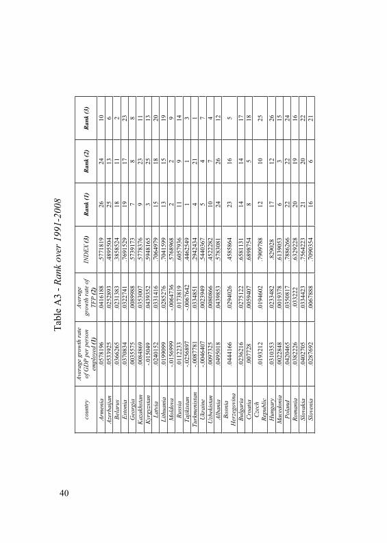
40
Tabl
e A
3 - R
ank
over
199
1-20
08
coun
try
Aver
age
grow
th ra
te
of G
DP
per p
erso
n em
ploy
ed (1
)
Aver
age
grow
th ra
te o
f TF
P(2
)IN
DEX
(3)
Ran
k (1
) R
ank
(2)
Ran
k (3
)
Arm
enia
.0
5781
96
.041
6188
.5
7718
19
26
24
10
Azer
baija
n .0
5339
25
.025
2893
.4
8955
04
25
13
6 Be
laru
s .0
3662
65
.023
1383
.3
8585
24
18
11
2 Es
toni
a .0
3708
34
.032
2741
.7
6915
29
19
17
23
Geo
rgia
.0
0355
75
.008
9988
.5
7391
73
7 8
8 K
azak
hsta
n .0
0848
69
.035
3007
.5
7783
76
9 23
11
K
yrgy
zsta
n -.0
1504
9 .0
4393
52
.594
8165
3
25
13
Latv
ia
.024
0152
.0
3314
16
.706
4979
15
18
20
Li
thua
nia
.019
9099
.0
2852
76
.704
1599
13
15
19
M
oldo
va
-.015
6999
-.0
0647
36
.576
8968
2
2 9
Russ
ia
.011
2233
.0
1738
19
.605
7936
11
9
14
Tajik
ista
n -.0
2568
97
-.006
7642
.4
4625
49
1 1
3 Tu
rkm
enis
tan
-.008
7781
.0
3348
51
.294
2434
4
21
1 U
krai
ne
-.004
6407
.0
0239
49
.544
0367
5
4 7
Uzb
ekis
tan
.009
7325
.0
0808
66
.452
2282
10
7
4 Al
bani
a .0
4950
18
.043
9853
.5
7830
81
24
26
12
Bosn
ia
Her
zego
vina
.0
4441
66
.029
4026
.4
5858
64
23
16
5
Bulg
aria
.0
2362
16
.027
5122
.6
5811
31
14
14
17
Cro
atia
.0
0772
8 .0
0594
07
.689
8754
8
5 18
C
zech
Re
publ
ic
.019
3212
.0
1946
02
.790
9788
12
10
25
Hun
gary
.0
3103
53
.023
3482
.8
2902
8 17
12
26
M
aced
onia
.0
0228
48
.001
9378
.6
1390
53
6 3
15
Pola
nd
.042
0465
.0
3508
17
.788
6266
22
22
24
Ro
man
ia
.038
2226
.0
3322
2 .6
3292
28
20
19
16
Slov
akia
.0
4027
05
.033
4423
.7
5642
23
21
20
22
Slov
enia
.0
2876
92
.006
7888
.7
0903
54
16
6 21
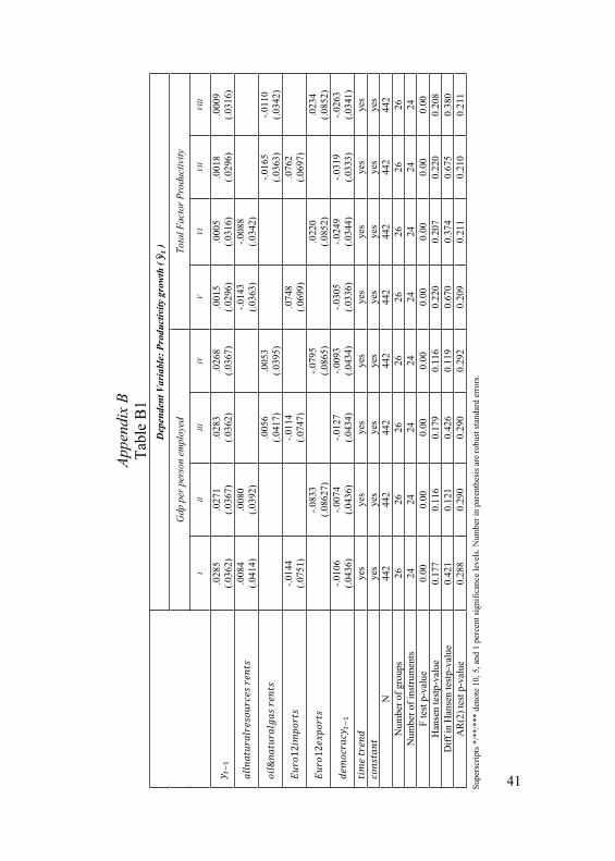
41
Appe
ndix
B
Tabl
e B
1 D
epen
dent
Var
iabl
e: P
rodu
ctiv
ity g
row
th (
)
Gdp
per
per
son
empl
oyed
To
tal F
acto
r Pro
duct
ivity
III
III
IVV
VIVI
IVI
II
.028
5
(.036
2)
.027
1
(.036
7)
.028
3
(.036
2)
.026
8
(.0
367)
.0
015
(.0
296)
.0
005
(.0
316)
.0
018
(.0
296)
.0
009
(.031
6)
.008
4
(.041
4)
.008
0
(.039
2)
-.014
3
(.036
3)
-.008
8
(.034
2)
.005
6
(.041
7).0
053
(.0
395)
-.0
165
(.0
363)
-.0
110
(.034
2)
-.014
4
(.075
1)
-.011
4
(.074
7).0
748
(.0
699)
.0
762
(.0
697)
-.0
833
(.0
8627
) -.0
795
(.0
865)
.0
220
(.0
852)
.0
234
(.0
852)
-.0
106
(.0
436)
-.0
074
(.0
436)
-.0
127
(.0
434)
-.009
3
(.043
4)
-.030
5
(.033
6)
-.024
9
(.034
4)
-.031
9
(.033
3)
-.026
3
(.034
1)
yes
yes
yes
yes
yes
yes
yes
yes
yes
yes
yes
yes
yes
yes
yes
yes
N
442
442
442
442
442
442
442
442
Num
ber o
f gro
ups
26
26
26
26
26
26
26
26
Num
ber o
f ins
trum
ents
24
24
24
24
24
24
24
24
F
test
p-v
alue
0.
00
0.00
0.
00
0.00
0.
00
0.00
0.
00
0.00
H
anse
n te
stp-
valu
e 0.
177
0.11
6 0.
179
0.11
6 0.
220
0.20
7 0.
220
0.20
8 D
iff in
Han
sen
test
p-va
lue
0.42
1 0.
121
0.42
6 0.
119
0.67
0 0.
374
0.67
5 0.
380
AR
(2) t
est p
-val
ue
0.28
8 0.
290
0.29
0 0.
292
0.20
9 0.
211
0.21
0 0.
211
Supe
rscr
ipts
*/*
*/**
* de
note
10,
5, a
nd 1
per
cent
sign
ifica
nce
leve
ls. N
umbe
r in
pare
nthe
sis a
re ro
bust
stan
dard
err
ors.

42
ReferencesAcemoglu D., Johnson S., Robinson J. A., and Yared P. (2008), “Income and Democracy”, American Economic Review, 98 (3), 808-842.
Acemoglu D., Johnson S., and Robinson J. A. (2005), “Institutions as the Fundamental Cause of Long-Run Growth”, Handbook of Economic Growth.
Acemoglu D. and Robinson J. A. (2008), “Persistence of Power,Elites and Institutions”, American Economic Review, 98 (1), 267-293.
Acemoglu D., Johnson S., and Robinson J. A. (2002), “Reversal of Fortune: Geography and Institutions in the Making of the Modern World Income Distribution”, Quarterly Journal of Economics, 117 (4), 1231-1294.
Acemoglu D., Johnson S., and Robinson J. A. (2005), “The Rise of Europe: Atlantic Trade, Institutional Change, and Economic Growth”, American Economic Review, 95 (3), 546-579.
Arellano M. and Bover O. (1995), “Another look at the instrumental variables estimation of error components models”, Journal of Econometrics, 68 (1), 29-52.
Arellano M. and Bond S. (1991), “Some tests of specification for panel data: Monte Carlo evidence and an application to employment equations”, Review of Economic Studies, 58 (2), 277-297.
Auty R. M. (2001), “The political economy of resource-driven growth”, European Economic Review, 45 (4-6), 839-846.
Auty R. M. And Gelb A. H. (2001), “Political Economy of resource-abundant states”, in Auty R. M. (ed.), Resource

43
Abundance and Economic Development, Oxford: Oxford University Press.
Barlow D. (2006), “Growth in Transition Economies: A Trade Policy Perspective”, Economics of Transition, 14 (3), 505-515.
Beck T. and Laeven L. (2006), “Institutions building and growth in transition economies”, Journal of Economic Growth, 11 (2), 157-186.
Berg A., Borensztein E., Sahay R., and Zettelmeyer J. (1999), “The Evolution of Output in Transition Economies: Explaining the Differences”, IMF Working Paper, WP/99/73, 1-81.
Blanchard O. and Kremer M. (1997), “Disorganization”, Quarterly Journal of Economics, 112 (4), 1091-1126.
Blanchard O. (1996), “Theoretical Aspects of Transition”, American Economic Review, 86 (2), 117-122.
Blundell R. and Bond S. (1998), “Initial conditions and moment restrictions in dynamic panel data models”, Journal of Econometrics, 87 (1), 115-143.
Bond S. (2002), “Dynamic panel data models: A guide to micro data methods and practice”, Working Paper CWP09/02, Cemmap, Institute for Fiscal Studies.
Bond S., Hoeffler A., and Temple J. (2001), “GMM estimation of empirical growth models”, CEPR Discussion Paper No. 3048.
Brunnschweiler C. N. (2009), “Oil and Growth in Transition Countries”, Working Paper 09/108, Center of Economic Research at ETH Zurich. Calvo G. And Coricelli F. (1996), “Credit Market Imperfections and Low-Output Equilibria in Economies in Transition”, in
44
Financial Factors in Economic Stabilization and Growth ed. Cambridge: Cambridge U. Press, 75-102.
Campos N. F. and Coricelli F. (2002), “Growth in Transition: what we know, what we don’t, and what we should”, Journal of Economic Literature, XL, 793-836.
Caselli F. (2005), “Accounting for cross-country income differences”, In: Aghion, P., Durlauf, S., (Eds.), Handbook of Economic Growth. New York: Elsevier, 679-741.
Dalmazzo A. and de Blasio G. (2001), “Resources and Incentives to Reform: A Model and Some Evidence on Sub-Saharan African Countries”, IMF Working Paper No. 86.
De Melo M., Denizer C., and Gelb A. (2001), “Circumstance and Choice: The Role of Initial Conditions and Policies in Transition Economies”, World Bank Economic Review, 15 (1), 1-31.
De Melo M., Denizer C., and Gelb A. (1996), “Patterns of Transition from Plan to Market”, World Bank Economic Review, 10 (3), 397-424.
Di Tommaso M. L., Raiser M., and Weeks M. (2007), “Home Grown or Imported? Initial Conditions, External Anchors and The Determinants of Institutional Reform in The Transition Economies”, Economic Journal, 117 (520), 858-881.
Drukker D. M. (2003), “Testing for serial correlation in linear panel-data models”,Stata Journal, 3 (2), 168-177.
Dufour J. M. (2003), “Identification, Weak Instruments and Statistical Inference in Econometrics”, Canadian Journal of Economics, 36 (4), 767-808. Easterly W., Ritzen J., and Woolcock M. (2006), “Social Cohesion, Institutions, and Growth”,Economics and Politics, 18 (2), 103-120.
45
Eicher T. S., García-Peñalosa C., and Teksoz U. (2006), “How Do Institutions Lead Some Countries to Produce So Much More Output per Worker than Others?”, in Institutions, Development and Economic Growth, MIT Press.
Eicher T. S. and Schreiber T. (2010), “Structural policies and growth: Time series evidence from a natural experiment”, Journal of Development Economics, 91, 169-179.
Esanov A., Raiser M., and Buiter W. (2001), “Nature’s blessing or nature’s curse: the political economy of transition in resource-based economies”, EBRD Working Paper No. 66.
European Bank for Reconstruction and Development (various years), “Transition Report”, London: European Bank for Reconstruction and Development.
Filer R. K. and Hanousek J. (2002), “Data Watch: Research Data from Transition Economies”, Journal of Economic Perspectives, 16 (1), 225-240.
Fischer S., Sahay R., and Végh C. A. (1996), “Economies in Transition: The Beginnings of Growth”, American Economic Review, 86 (2), 229-233.
Fischer S., Sahay R., and Végh C. A. (1996), “Stabilization and Growth in Transition Economies: The Early Experience”, Journal of Economic Perspectives, 10 (2), 45-66.
Fischer S. and Sahay R. (2000), “The Transition Economies After Ten Years”, NBER Working Paper No. 7664, 1-43.
Frees E. W. (1995), “Assessing cross-sectional correlations in panel data”, Journal of Econometrics, 69 (2), 393-414.
46
Frees E. W. (2004), “Longitudinal and panel data: analysis and applications in the social sciences”, Cambridge University Press.
Gaddy C. and Ickes B. (1998), “Beyond a Bail Out: Time to Face Reality about Russia’s ‘Virtual Economy’”, mimeo, Brookings Institution.
Glaeser E. L., La Porta R., Lopez-de-Silanes F., and Shleifer A. (2004), “Do Institutions Cause Growth?”, Journal of Economic Growth, 9 (3), 271-303.
Goel R. K. and Budak J. (2006), “Corruption in Transition Economies: Effects of Government Size, Country Size and Economic Reforms”, Journal of Economics and Finance, 30 (2), 240-250.
Gomulka S. (1994), “Economic and Political Constraints during Transition”, Europe-Asia Studies, 46 (1), 89-106.
Greene W. H. (2007), “Econometric Analysis”, 6th ed. Upper Saddle River, NJ: Prentice Hall.
Gylfason T. (2001), “Natural Resources and Economic Growth: What Is the Connection?”, CESifo Working Paper No. 530.
Hall R. E. and Jones C. I. (1999), “Why Do Some Countries Produce So Much More Output than Others?”, Quarterly Journal of Economics, 114 (1), 83-116.
Havrylyshyn O. and Van Rooden R. (2003), “Institutions Matter in Transition, But So Do Policies”, Comparative Economic Studies, 45, 2-24. Hoff K. and Stiglitz J. E. (2002), “After the Big Bang? Obstacles to the Emergence of the Rule of Law in Post-Communist Societies”, American Economic Review, 94 (3), 753-763.
47
Holtz-Eakin, D., W. Newey, and H. S. Rosen. (1988), “Estimating vector autoregressions with panel data”, Econometrica, 56, 1371-1395.
Im K. S., Pesaran M. H., and Shin Y. (2003), “Testing for unit roots in heterogeneous panels”, Journal of Econometrics, 115 (1), 53–74.
Kaminski B. (1996), “Factors affecting trade reorientation in the newly independent states”, in Kaminski B. (ed.), Economic Transition in Russia and the New States of Eurasia, New York, NY: Sharpe.
Kaminski B., Wang Z. K. And Winters L. A. (1996), “Foreign trade in the transition: The international environment and domestic policy”, Studies in Economies in Transformation, 20, Washington, DC: World Bank.
Kenez P. (2006), “A History of the Soviet Union from the Beginning to the End”, Cambridge University Press.
Khanin G. I. (1991), “Economic Growth in the USSR in the Eighties”, Ekonomika i organizatsiyapromyshlennogoproizvodstva, 5, 25-34. A publication of the Institute of the Economics and Organization of Industrial Production, Siberian Division, USSR Academy of Sciences.
Kronenberg T. (2004), “The curse of natural resources in the transition economies”, Economics of Transition, 12 (3), 399-426.
Kudrov V. (1994), “Are the Calculations of Economic Growth Rates for the USSR and Russia Reliable?”, VoprosyEkonomiki, 10, 122-131. (A publication of the Institute of Economics, Russian Academy of Sciences).
48
Lee Y.-S. and Jeong H.-G. (2006), “The Determinants of Economic Growth of Transition Economies: Economic Reform versus Initial Conditions”, International Economic Journal, 20 (2), 241-252.
Levin A., Lin C.-F., and Chu C.-S. J. (2002), “Unit root tests in panel data: Asymptotic and finite-sample properties”, Journal of Econometrics, 108 (1), 1–24.
Luintel K.B. and Khan, M. (2004), “Are international R&D spillovers costly for the United States?”, The Review of Economics and Statistics, 86, 896-910.
Marin D. and Schnitzer M. (1999), “Disorganization and Financial Collapse”, CEPR discuss. Paper 1580.
Mikesell R. F. (1997), “Explaining the resource curse, with special reference to mineral-exporting countries”, Resources Policy, 23(4), 191-99.
Nelson R. (2007), “Institutions and Economic Growth: Sharpening the Research Agenda”, Journal of Economic Issues, 41 (2), 313-323.
North D. C. (1971), “Institutional Change and Economic Growth”, Journal of Economic History, 31 (1), 118-125.
North D. C. (1991), “Institutions”, Journal of Economic Perspectives, 5 (1), 97-112.
North D. C. (1990), “Institutions, Institutional Change and Economic Performance”, Cambridge University Press.
Ofer G. (1987), “Soviet Economic Growth: 1928-1985”, Journal of Economic Literature, 25 (4), 1767-1833.
49
Parente S. L. and Ríos-Rull J.-V. (2005), “The Success and Failure of Reforms in Transition Economies”, Journal of Money, Credit, and Banking, 37 (1), 24-42.
Pesaran M. H. (2004), “General diagnostic tests for cross section dependence in panels”, Cambridge Working Papers in Economics, 0435, University of Cambridge.
Pistor K., Raiser M., and Gelfer S. (2000), “Law and Finance in Transition Economies”, Economics of Transition, 8 (2), 325-368.
Rodrik D. and Wacziarg R. (2005), “Do Democratic Transitions Produce Bad Economic Outcomes?”, American Economic Review, 95 (2), 50-55.
Rodrik D. (2007), “One economics, Many Recipes”, Princeton University Press.
Rodrik D. (2008), “Second-Best Institutions”, American Economic Review, 98 (2), 100-104.
Roodman D. (2009), “A note on the theme of too many instruments”, Oxford Bulletin of Economics and Statistics 71 (1), 135-158.
Roodman, D. (2006), “How to Do xtabond2: An introduction to "Difference" and "System" GMM in Stata”, Working Paper 103, Center for Global Development, Washington.
Sachs J. D. and Warner A. M. (1995), “Natural Resource Abundance and Economic Growth”, NBER Working Paper 5398, Cambridge, Massachusetts.
Sachs J. D. and Warner A. M. (2001), “The curse of natural resources”, European Economic Review, 45, 827-838.

50
Sala-i-Martin X. (1997), “I just ran two million regressions”, American Economic Review, 87(2), 178-83.
Sarafidis V. and De Hoyos R. E. (2006), “On testing for cross sectional dependence in panel data models”, Stata Journal, 6 (4), 482-496.
Selowsky M. and Martin R. (1997), “Policy Performance and Output Growth in the Transition Economies”, American Economic Review, 87 (2), 349-353.
Shea J. (1997), “Instrument relevance in multivariate linear models: A simple measure”, Review of Economics and Statistics, 79 (2), 348-352.
Staehr K. (2005), “Reforms and Economic Growth in Transition Economies: Complementarity, Sequencing and Speed”, The European Journal of Comparative Economics, 2 (2), 177-202.
Stock J. H. and Wright J. H. (2000), “GMM with weak identification”, Econometrica, 68 (5), 1055-1096.
Stock J. H. and Yogo M. (2005), “Testing for weak instruments in linear IV regression”, in Identification and Inference for Econometric Models: Essays in Honor of Thomas Rothenberg, ed. D. W. K. Andrews and J. H. Stock, 80-108. Cambridge: Cambridge University Press.
Sušjan A. and Redek T. (2005), “The Impact of Institutions on Economic Growth: The Case of Transition Economies”, Journal of Economic Issues, 39 (4), 995-1027.
Sušjan A. and Redek T. (2008), “Uncertainty and Growth in Transition Economies”, Review of Social Economy, 66 (2), 209-234.
51
Svejnar J. (2002), “Transition Economies: Performance and Challenges”, Journal of Economic Perspectives, 16 (1), 3-28.
Vieira F., MacDonald R.,and Damasceno A. (2012), “The role of institutions in cross-section income and panel data growth models: A deeper investigation on the weakness and proliferation of instruments”, Journal of Comparative Economics 40, 127-140.
Windmeijer F. (2005),”A finite sample correction for the variance of linear efficient two-step GMM estimators”, Journal of Econometrics, 126 (1), 25-51.
Wooldridge J. M. (2010), “Econometric Analysis of Cross Section and Panel Data”, MIT press.
Wooldridge J. M. (2005), “Instrumental Variables Estimation with Panel Data”, Econometric Theory, 21, 865-869.

52
Elenco Quaderni già pubblicati
1. Capitalismo senza capitale. Il capitalismo italiano delle diversità.L. Campiglio, luglio 1993.
2. Credibility and Populism in the Management of a Public Social Security System. L. Bonatti, luglio 1993.
3. Il ruolo delle NonprofitOrganizations nella produzione di servizi sanitari.R. Creatini, dicembre 1993.
4. Technological Change, Diffusion and Output Growth. M. Baussola, dicembre 1993.
5. Europe: the Trademark is Still on the Mark. L.Campiglio, gennaio 1994.
6. A Cointegration Approach to the Monetary Model of the Exchange Rate. M. Arnone, febbraio 1994.
7. Gli effetti del debito pubblico quando la ricchezza è un fine e non solo un mezzo. V. Moramarco, maggio 1994.
8. Emissioni inquinanti, asimmetria informativa ed efficacia delle imposte correttive. R. Creatini, settembre 1994.
9. La disoccupazione in Europa. L. Campiglio, novembre 1994. 10. The Economics of Voting and Non-Voting: Democracy and
Economic Efficiency. L. Campiglio, gennaio 1995. 11. The Banking Law and its Influence on the Evolution of the
Italian Financial System. C. Bellavite Pellegrini, maggio 1995.
12. Monetary Authorities, Economic Policy and Influences in the Capital Market in Italy 1960-1982. C. Bellavite Pellegrini, giugno 1995.
13. A General Model to Study Alternative Approaches to Economywide Models in a Transaction Values (TV) Context.F. Timpano, giugno 1995.
14. Economia legale ed economia illegale: schemi interpretativi della coesistenza. D. Marino, F. Timpano, luglio 1995.
53
15. Il problema del cambiamento dei coefficienti nel contesto di una matrice di contabilità sociale regionalizzata. F. Timpano, settembre 1995.
16. La dimensione transnazionale dell’inquinamento marino: le convenzioni internazionali tra teoria e pratica. G. Malerba, giugno 1996.
17. Efficienza, stabilità degli intermediari e crescita del reddito: un modello teorico. C. Bellavite Pellegrini, novembre 1996.
18. Innovation and the World Economy: How will our (Grand) Children Earn a Living?, L. Campiglio, P. J. Hammond, gennaio 1997.
19. Evaluating Private Intergenerational Transfers between Households. The Case of Italy. F. Tartamella, febbraio 1997.
20. Qualità e regolamentazione. R. Creatini, maggio 1997. 21. Wage Differentials, the Profit-Wage Relationship and the
Minimum Wage. G. Quintini, giugno 1997. 22. Potere e rappresentatività nel Parlamento Italiano: una
prospettiva economica. L. Campiglio, luglio 1997. 23. Exchange Rate, Herd Behaviour and Multiple Equilibria. M.
Arnone, settembre 1997. 24. Rank, Stock, Order and Epidemic Effects in the Diffusion of
New Technologies in Italian Manufacturing Industries. E. Bartoloni, M. Baussola, dicembre 1997.
25. Stabilità ed Efficienza del Sistema Finanziario Italiano: una Verifica Empirica. M. Manera, C. Bellavite Pellegrini, gennaio 1998.
26. EndogenousUncertainty and Market Volatility. M. Kurz, M. Motolese, aprile 1999.
27. Famiglia, distribuzione del reddito e politiche familiari: una survey della letteratura degli anni Novanta. Parte prima: I nuovi fenomeni e i vecchi squilibri delle politiche sociali. G. Malerba, aprile 2000.
28. Modelli di Agenzie di sviluppo regionale: analisi teorica ed evidenza empirica. M. Arnone, C. Bellavite Pellegrini, F. Timpano, aprile 2000.
54
29. Endogenous Uncertainty and the Non-neutrality of Money. M. Motolese, maggio 2000.
30. Growth, Persistent Regional Disparities and Monetary Policy in a Model with Imperfect Labor Markets. L. Bonatti, maggio 2001.
31. Two Arguments against the Effectiveness of Mandatory Reductions in the Workweek as a Job Creation Policy. L. Bonatti, maggio 2001.
32. Growth and Employment Differentials under Alternative Wage-Setting Institutions and Integrated Capital Markets. L. Bonatti, maggio 2001.
33. Attività innovativa e spillovers tecnologici: una rassegna dell'analisi teorica. A. Guarino, maggio 2001.
34. Famiglia, distribuzione del reddito e politiche familiari: una survey della letteratura italiana degli anni Novanta. Parte seconda: La riforma del Welfare e le sue contraddizioni. G. Malerba, giugno 2001.
35. Changeover e inflazione a Milano. L. Campiglio, V. Negri, giugno 2002.
36. Prezzi e inflazione nel mercato dell’auto in Italia. L. Campiglio, A. Longhi, ottobre 2002.
37. Interessi economici, potere politico e rappresentanza parlamentare in Italia nel periodo 1948-2002. L. Campiglio, F. Lipari, maggio 2003.
38. Dai consumi interni a quelli dei residenti: una stima preliminare a livello regionale. C. Corea, giugno 2003.
39. Studio delle relazioni tra spesa familiare e caratteri sociali, demografici ed economici delle famiglie italiane: un’analisi a livello sub-nazionale. A. Coli, giugno 2003.
40. L’utilizzo delle indagini su redditi e consumi nella derivazione di indicatori per scomporre i dati di Contabilità Nazionale. Un caso riferito all’analisi regionale. F. Tartamella, giugno 2003.
41. Segnali di disagio economico nel tenore di vita delle famiglie italiane: un confronto tra regioni. G. Malerba, S. Platoni, luglio 2003.
55
42. Rational Overconfidence and Excess Volatility in General Equilibrium. C.K. Nielsen, febbraio 2004.
43. How Ethnic Fragmentation And Cultural Distance Affect Moral Hazard in Developing Countries: a Theoretical Analysis. T. Gabrieli, febbraio 2004.
44. Industrial Agglomeration: Economic Geography, Technological Spillover, and Policy incentives. E. Bracco, ottobre 2005.
45. An Introduction to the Economics of Conflict, a Survey of Theoretical Economic Models of Conflict. R. Caruso, ottobre 2005.
46. A Model of Conflict with Institutional Constraint in a two-period Setting. What is a Credible Grant?, R. Caruso, ottobre 2005.
47. On the Concept of Administered Prices. L. Gattini, dicembre 2005.
48. Architecture of Financial Supervisory Authorities and the Basel Core Principles. M. Arnone, A. Gambini, marzo 2006.
49. Optimal Economic Institutions Under Rational Overconfidence. With applications to The Choice of Exchange Rate Regime and the Design of Social Security. C.K. Nielsen, aprile 2006.
50. Indicatori di vulnerabilità economica nelle regioni italiane: un’analisi dei bilanci familiari. G. Malerba, giugno 2006.
51. Risk Premia, Diverse Beliefs and Beauty Contests. M. Kurz, M. Motolese, gennaio 2007.
52. Le disuguaglianze regionali nella distribuzione del reddito. Parte prima: Un’analisi della povertà delle famiglie italiane.G. Malerba, dicembre 2009.
53. What do we know about the link between growth and institutions?, M. Spreafico,maggio 2010.
54. Economic Institutions and Economic Growth in the Former Soviet Union Economies. M. Spreafico, maggio 2010.
55. Famiglia, figli e sviluppo sostenibile. L. Campiglio, settembre 2011.
56
56. Le determinanti politico-economiche della distribuzione interregionale della spesa pubblica. V. Moramarco, ottobre 2011.
57. Le disuguaglianze regionali nella distribuzione del reddito. Parte seconda: Un’analisi delle famiglie italiane a rischio di povertà. G. Malerba, ottobre 2011.
58. Libertà del vivere una vita civile e deprivazione economica. L. Campiglio, ottobre 2011.
59. Europa, crescita e sostenibilità: “E Pluribus Unum”. L. Campiglio, Vita e Pensiero, febbraio 2012 (ISBN 978-88-343-2215-4).
60. Market’s SINS and the European Welfare State: theory and empirical evidences. L. Campiglio, Vita e Pensiero, settembre 2012 (ISBN 978-88-343-2323-6).
61. Brutality of JihadistTerrorism. A contest theory perspective and empirical evidence in the period 2002-2010. R. Caruso, F. Schneider, Vita e Pensiero, ottobre 2012 (ISBN 978-88-343-2360-1).
62. Hooliganism and demand for football in Italy. Evidence for the period 1962-2011.R. Caruso, M. di Domizio, Vita e Pensiero, novembre 2012 (ISBN 978-88-343-2368-7).
63. WhyItaly’ssaving rate became (so) low?, L. Campiglio, Vita e Pensiero, febbraio 2013 (ISBN 978-88-343-2500-1).
64. Institutions, the resource curse and the transition economies: further evidence, M. Spreafico, Vita e Pensiero, aprile 2013 (ISBN 978-88-343-2551-3).

57

58
Printed by Gi&Gi srl - Triuggio (MB)
April 2013

ISTITUTO DI POLITICA ECONOMICA
Institutions, there source curse and the transition economies:
further evidence
Marta Spreafico
Quaderno n. 64/aprile 2013
VITA E PENSIERO
788834 3255139 >
ISBN 978-88-343-2551-3
COP Spreafico.qxd:_ 10/04/13 11:38 Page 1
Top Related