


Languages
Pages
Legal


1
Institutional similarity, Institutions� quality and trade.
Emmanuelle Lavallée
EURIsCO
Université Paris Dauphine
Place du Maréchal de Lattre de Tassigny
75016 PARIS
Mail : [email protected]
RESUME :
This paper uses a gravity model to assess the impact on trade of the proximity and the quality
of institutions. A new index of institutional similarity is proposed. It is computed on the basis
of data on national legal traditions.
The model includes 145 countries and is estimated with panel data over the period 1984-2002.
The estimation results clearly show that institutional proximity increases bilateral trade.
However, this paper leads to reconsider the impact of bad governance, and especially of
corruption on international trade. Indeed, the results show that the consequences on trade of
institutions� quality are more complex than the recent literature has suggested it.
2
I INTRODUCTION
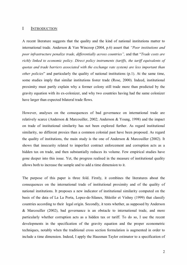
A recent literature suggests that the quality and the kind of national institutions matter to
international trade. Anderson & Van Wincoop (2004, p.6) assert that �Poor institutions and
poor infrastructure penalize trade, differentially across countries�, and that �Trade costs are
richly linked to economic policy. Direct policy instruments (tariffs, the tariff equivalents of
quotas and trade barriers associated with the exchange rate system) are less important than
other policies� and particularly the quality of national institutions (p.1). At the same time,
some studies imply that similar institutions foster trade (Rose, 2000). Indeed, institutional
proximity must partly explain why a former colony still trade more than predicted by the
gravity equation with its ex-colonizer, and why two countries having had the same colonizer
have larger than expected bilateral trade flows.
However, analyses on the consequences of bad governance on international trade are
relatively scarce (Anderson & Marcouiller, 2002; Anderson & Young, 1998) and the impact
on trade of institutional similarity has not been explored further. As regard institutional
similarity, no different proxies than a common colonial past have been proposed. As regard
the quality of institutions, the main study is the one of Anderson & Marcouiller (2002). It
shows that insecurity related to imperfect contract enforcement and corruption acts as a
hidden tax on trade, and then substantially reduces its volume. Few empirical studies have
gone deeper into this issue. Yet, the progress realised in the measure of institutional quality
allows both to increase the sample and to add a time dimension to it.
The purpose of this paper is three fold. Firstly, it combines the literatures about the
consequences on the international trade of institutional proximity and of the quality of
national institutions. It proposes a new indicator of institutional similarity computed on the
basis of the data of La La Porta, Lopez-de-Silanes, Shleifer et Vishny (1999) that classify
countries according to their legal origin. Secondly, it tests whether, as supposed by Anderson
& Marcouiller (2002), bad governance is an obstacle to international trade, and more
particularly whether corruption acts as a hidden tax or tariff. To do so, I use the recent
developments in the specification of the gravity equation and the proper econometric
techniques, notably when the traditional cross section formulation is augmented in order to
include a time dimension. Indeed, I apply the Hausman Taylor estimator to a specification of

3
the gravity equation extracted from Anderson and Van Wincoop (2003, 2004) which
explicitly includes a trade cost function inspired by Anderson & Marcouiller (2002). Thirdly,
I propose an alternative vision of the consequences of bad governance on international trade
which allows the interaction between corruption and the others aspects of governance. This
specification intends to assess second best theories that consider corruption as way to bypass
rigidities imposed by governments.
Section two presents the recent literature on the impact on trade of institutional similarity and
of the quality of national institutions. Section three explains the specification of the gravity
equation and the estimation technique. Section four present our first results. Section five tests
an alternative view of the consequences of weak national institutions on trade. Section six,
concludes.
II NATIONAL INSTITUTIONS AND INTERNATIONAL TRADE
The sort and the quality of national institutions appear to impact dramatically international
trade.
According to Disdier & Mayer (2005), the kind of national institutions and more specifically
similarity between institutional frameworks can explain the important and robust impact of
colonial links on bilateral exchanges1. Such institutions involve legal rules and administrative
systems. Sharing similar institutional frameworks can ease international trade by improving
contract enforcement and reducing transaction costs. However, the colonial relationship
captures other phenomenon. Indeed, it also reveals the existence of formal or informal
networks. Colonizers have usually established trade networks in their colonies, and those
networks can persist even after the decolonization. The explanatory power of international
migration patterns should not be neglected either. Lastly, colonial links don�t exhaust every
case of institutional similarity. Indeed, countries having had no colonial relationship can have
the same institutional framework. As such, national laws are fine examples. They are typically
not written from scratch, but rather transplanted from a few legal families or traditions
(Waston,1974; La Porta, Lopez de Silanes, Shleifer & Vishny). Those families or traditions
1 Rose (2000) shows that, for the year 2000, that, everything else equal, the colonial link increases trade by a factor 5.75, while having had a common colonizer raises countries bilateral trade by 80%.

4
have spread around the world through a combination of conquest, colonisation, imitation or
voluntary adoption. That is why this article investigates the consequences on international
trade of institutional similarity with new indicator. It is computed on the basis of the data of
La Porta, Lopez de Silanes, Shleifer & Vishny (1999) on countries� legal origin. It
distinguishes five national commercial legal traditions: common law, French civil law,
German civil law, Scandinavian law and socialist law. The variable of institutional similarity
takes the value of one if the national laws of the trading partners have the same legal origin
and zero otherwise.
Anderson and Marcouiller (2002) first demonstrate the importance of strong institutions on
international trade. They build a model of import demand in an insecure world. They show
that predation by thieves or by corrupt officials generates a price mark-up equivalent to a
hidden tax or tariff, which extent depends on the quality of institutions for the defence of
trade. This price mark-up significantly constrains trade by two channels: a substitution effect
between traded goods and non traded goods, and a real income effect. Anderson and
Marcouiller�s structural model is quite singular. Indeed, they use a variant of the traditional
gravity model: they divide imports of j from i by k imports from i, which cancels the exporter
price index. The importer relative price index is approximated with a Törnqvist index.
Working on relative imports addresses a specification error that plagues many empirical
studies, i.e. the estimation of highly non linear specific exporter and importer price indexes.
In order to estimate their model, the authors use data provided by the World Economic Forum
(WEF) to evaluate the strength of national institutions for the defence of trade. They test the
model for the year 1996 for a sample of 48 importing countries, half of them being developed
countries. They find that trade increases dramatically when it is supported by strong
institutions. They conclude that: �If the seven Latin American countries of the sample were to
enjoy the same transparency and enforceability scores as the mean scores of the members of
the European Union, predicted Latin American imports volume would rise by 30%� (p349).
However, this literature leaves out �second best� theories which regard corruption as a
�beneficial grease� for trade. Indeed, �second best� analysis see corruption as a way to bypass
rigidities imposed by governments. Bhagwati (1982, p. 993) suggests that corruption must be
analysed as a Directly Unproductive Profit-seeking activity (DUP), that is to say a way �of
making profits by undertaking activities that are directly unproductive�(p989). In the area of
international trade, corruption can be compared to others DUP activities such as tariff evasion
or smuggling. As long as these activities occur in initially distorted situations, second best

5
analysis applies and DUP should enhance welfare. Although, such theories do not directly
study the effect of corruption on the volume of international trade, they present corruption as a
mean of greasing the wheels of commerce.
Next section�s objective is to specify gravity models so as to test just as well Anderson &
Marcouiller�s view, as �second best� theories. To do so, I use the recent developments in the
specification of the gravity equation and the proper econometric techniques, notably when the
traditional cross section formulation is augmented in order to include a time dimension.
Indeed, our gravity models include 144 countries and are estimated with panel data over the
period 1984-2002.
III SPECIFICATION OF THE GRAVITY EQUATION AND DATA
A Trade barriers and gravity equation
I use the specification of the gravity equation of Anderson & Van Wincoop (2003, 2004).
Anderson & Van Wincoop demonstrate that, in a one sector economy, when consumers have
CES preferences with common elasticity among all goods, the gravity equation can be written
as:
σ−
ΠΠ=
1
jP
i
ijt
wY
jY
iY
ijX (1)
j1ij
tii
1i
1j
P ∀σ−θ∑ −σΠ=σ− (2)
σ−∑ θ−σ=σ−Π 1ij
tj j
1j
P1i
(3)
Where Yi et Yj are levels of GDP, Yw is world GDP, et θi is income share of country i, et tij is
trade costs. With symmetry of trade costs (tij = tji), then Пi=Pi, and equation (1) then becomes:
σ−
=
1
jP
iP
ijt
wY
jY
iY
ijX (4)
6
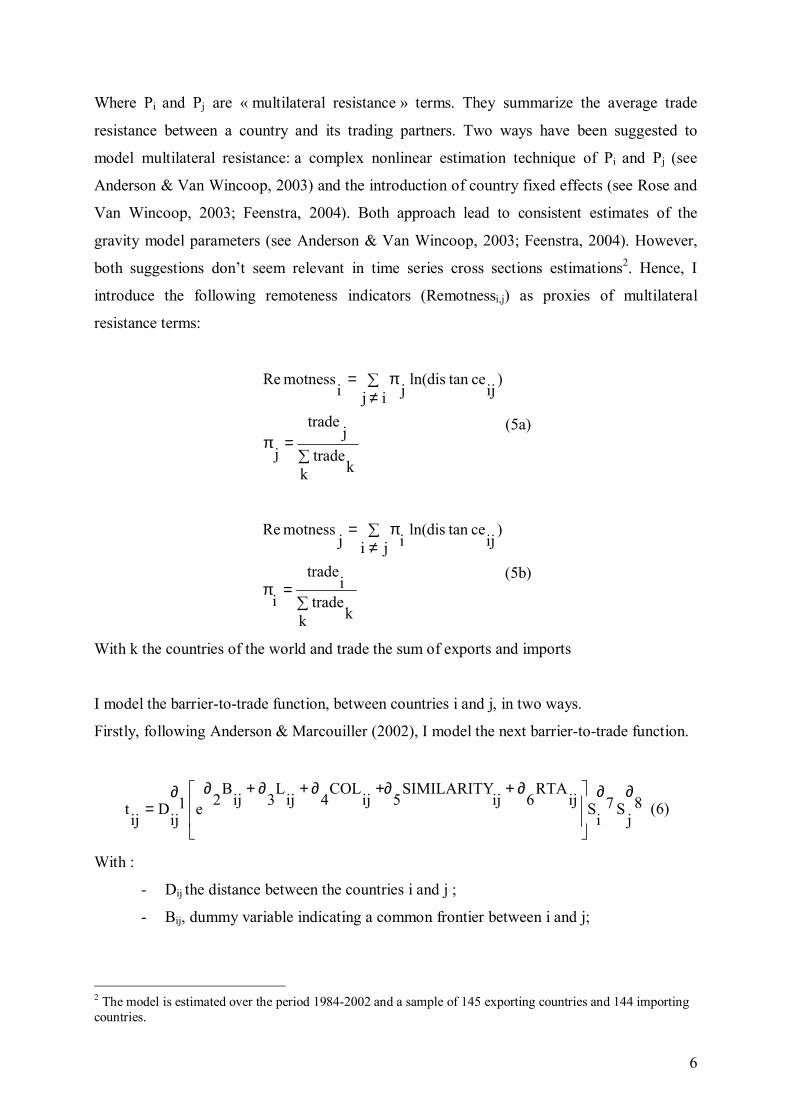
Where Pi and Pj are « multilateral resistance » terms. They summarize the average trade
resistance between a country and its trading partners. Two ways have been suggested to
model multilateral resistance: a complex nonlinear estimation technique of Pi and Pj (see
Anderson & Van Wincoop, 2003) and the introduction of country fixed effects (see Rose and
Van Wincoop, 2003; Feenstra, 2004). Both approach lead to consistent estimates of the
gravity model parameters (see Anderson & Van Wincoop, 2003; Feenstra, 2004). However,
both suggestions don�t seem relevant in time series cross sections estimations2. Hence, I
introduce the following remoteness indicators (Remotnessi,j) as proxies of multilateral
resistance terms:
∑=π
∑≠
π=
k ktrade
jtrade
j
)ij
cetandisln(ij ji
motnessRe
(5a)
∑=π
∑≠
π=
k ktrade
itrade
i
)ij
cetandisln(ji ij
motnessRe
(5b)
With k the countries of the world and trade the sum of exports and imports
I model the barrier-to-trade function, between countries i and j, in two ways.
Firstly, following Anderson & Marcouiller (2002), I model the next barrier-to-trade function.
8j
S7i
SijRTA
6ijSIMILARITY
5ijCOL
4ijL
3ijB
2e1ij
Dij
t∂∂
∂++∂∂+∂+∂∂= (6)
With :
- Dij the distance between the countries i and j ;
- Bij, dummy variable indicating a common frontier between i and j;
2 The model is estimated over the period 1984-2002 and a sample of 145 exporting countries and 144 importing countries.

7
- Lij a dummy variable that takes the value of one if the two trading partners share a
common language and zero otherwise;
- COLij is a binary variable which is equal unity if i ever colonized j and vice versa.
- SIMILARITYij is a dummy variable equals to one if the trading partners have
similar institutions and zero otherwise ;
- RTAij dummy variable indicating a common belonging to a preferential trade
agreement (RTAij).
- Si(j) the quality of institutions of country i(j).
In this formulation, weak national institutions raise trade costs. Increasing distance between
trading partners increase transport costs. However, if the importer and the exporter share a
common border, a common language, a colonial past or similar institutions that encourage
familiarity and may enhance the importer and the exporter�s skills in using the institutions of
its partner and then decrease transactions costs. Lastly, the belonging to a common
preferential trade agreement may reduce trade costs.
Secondly, in order to test specifically �second best� theories, I introduce the following
barrier-to-trade function. In comparison with the previous formulation, it has the distinctive
feature of allowing interactions between the corruption and the other elements of governance.
)j
Sln109
(
jCOR
)i
Sln87
(
iCOR
ijRTA
6ijSIMILARITY
5ijCOL
4ijL
3ijB
2e1ij
Dij
t
∂+∂×
∂+∂×
∂++∂∂+∂+∂∂=
(7)
Where :
- CORi(j) the level of corruption in country i(j) ;
- Si(j) the quality of institutions (without corruption)in country i(j) ;
- Other variables are defined as in equation (7)
Substituting equation (6) into (4) and taking logs,
ijw
jSln
12iSln
11ijRTA
10
ijSIMILARITY
9ijCOL
8ijL
7ijB
6ijDln
5
jmotnessRe
4imotnessReln
3jYln
2iYln
10ijXln
+β+β+β+
β+β+β+β+β+
β+β+β+β+β=
(8)

8
Where the world GDP is absorbed in the constant error term, wij is the error term, and with
the expected signs3 :
( ) ( )( ) ( ) ( )( ) ( ) ( ) 0
81
12;0
71
11;0
61
10
;05
19
;04
18
;03
17
;02
16
;01
15
;04
;03
;02
;01
>∂σ−=β>∂σ−=β>∂σ−=β
>∂σ−=β>∂σ−=β>∂σ−=β
>∂σ−=β>∂σ−=β<β<β>β>β
Similarly, substituting equation (7) into (4) and taking logs, the gravity equation becomes:
ijw
jCORln)
jSln
1413(
iCORln)
iSln
1211(
ijRTA
10
ijSIMILARITY
9ijCOL
8ijL
7ijB
6ijDln
5
jmotnessRe
4imotnessReln
3jYln
2iYln
10ijXln
+β+β+β+β+β+
β+β+β+β+β+
β+β+β+β+β=
(9)
The expected signs of parameters β1 to β10 are the same as in equation (8). One the other hand,
the �grease the wheels hypothesis� will not be rejected if β11 and β13 are positive and β12 and
β14 are negative. Indeed, under the �grease the wheels� hypothesis corruption shall have a
positive impact on trade if the quality of governance if very law. Law quality of governance
implies lnSi(j) close to zero. With lnSi(j) close to zero, β11(13) must be positive for corruption to
have a positive impact on bilateral trade. With high quality of governance the impact of
corruption will become negative. In order to get such impact, β12(14) must be negative.
B Panel specification
In order to take into account exports flows� heterogeneity, I estimate my gravity equation with
panel data model. They enable to identify the country pair specific effect and to isolate them4.
The model (8) specified for panel data becomes:
ijtv
ijijtRERln
12ijCOL
11ijRTA
10
ijL
9ijB
8ijDln
7jSln
6iSln
5
jmotnessRe
4imotnessReln
3jYln
2iYln
1t0ijXln
+µ+α+α+α+
α+α+α+α+α+
α+α+α+α+α+α=
(10)
3The model proposed by Anderson & van Wincoop (2003) imposes the constraint, 1
21=β=β . But, here, this
constraint is relaxed. 4 A model with three specific effects: exporter, importer and time is only a restricted version of the more general model which allows country pair heterogeneity adopted here ( Carrère, 2005; Cheng & Wall, 1999; Endoh, 1999)
9
The model (9) specified for panel data becomes:
ijtv
ijijtRERln
14ijCOL
13ijRTA
12
ijL
11ijB
10ijDln
9jCORln)
jSln
87(
iCORln)
iSln
65(
jmotnessRe
4imotnessReln
3jYln
2iYln
1t0ijXln
+µ+α+α+α+
α+α+α+α+α+α+α+
α+α+α+α+α+α=
(11)
Where :
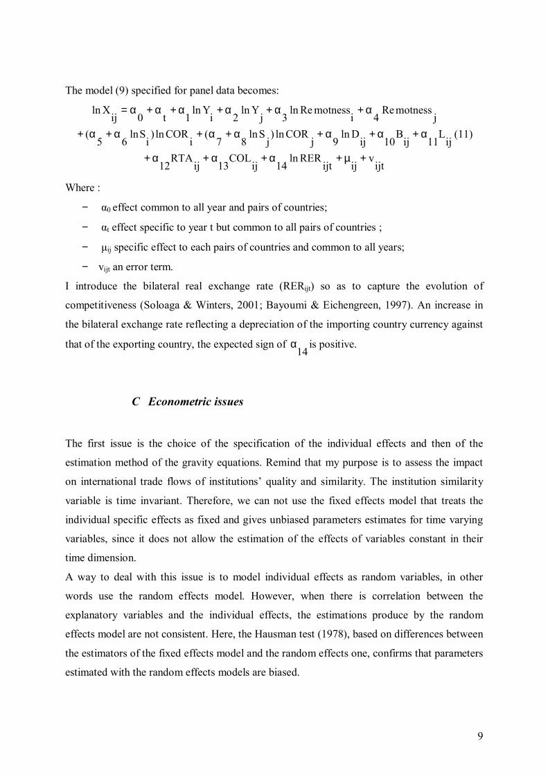
− α0 effect common to all year and pairs of countries;
− αt effect specific to year t but common to all pairs of countries ;
− µij specific effect to each pairs of countries and common to all years;
− vijt an error term.
I introduce the bilateral real exchange rate (RERijt) so as to capture the evolution of
competitiveness (Soloaga & Winters, 2001; Bayoumi & Eichengreen, 1997). An increase in
the bilateral exchange rate reflecting a depreciation of the importing country currency against
that of the exporting country, the expected sign of 14
α is positive.
C Econometric issues
The first issue is the choice of the specification of the individual effects and then of the
estimation method of the gravity equations. Remind that my purpose is to assess the impact
on international trade flows of institutions� quality and similarity. The institution similarity
variable is time invariant. Therefore, we can not use the fixed effects model that treats the
individual specific effects as fixed and gives unbiased parameters estimates for time varying
variables, since it does not allow the estimation of the effects of variables constant in their
time dimension.
A way to deal with this issue is to model individual effects as random variables, in other
words use the random effects model. However, when there is correlation between the
explanatory variables and the individual effects, the estimations produce by the random
effects model are not consistent. Here, the Hausman test (1978), based on differences between
the estimators of the fixed effects model and the random effects one, confirms that parameters
estimated with the random effects models are biased.

10
So as to tackle this problem, I use the Hausman Taylor estimator5(HT). Hausman & Taylor
(1978) propose an instrumental variable estimator that enables to estimate the parameters of
time invariant variables, and where some explanatory variables are correlated with individual
specific effects. The Hausman & Taylor estimator allows the estimation of consistent
parameters for time varying and time invariant explanatory variables. The definition of
independent variables as exogenous or endogenous is tested by a Hausman test of over-
identification, based on the comparison of the Hausman Taylor estimator and the within
estimator (estimator of the fixed effects model).
The second issue is the existence of zero export flows which can lead to selection bias6. Many
approaches have been suggested in the literature: replace them by small values, use TOBIT
models, use (1 + Xijt) rather than Xijt as trade measure. Here, I use a method applied by
Carrere (2005) to test and to correct a potential selection bias. This method, proposed by
Nijman & Verbeek (1992), approximates the Heckman correction term by adding variables
that reflects the presence of each country pair in the sample. The flowing variables are added:
• PRES: number of year of presence of the pair ij in the sample;
• DD: dummy variable that takes the value of one if the pair ij is observed during the
entire period, and zero otherwise;
• PAt: dummy variable that takes the value of one if ij was present in t-1, and zero
otherwise.
D Data7
Data on governance are extracted from the International Country Risk Guide�s (IRCG). They
are available over the period 1984-2002. More precisely, we use three IRCG ratings:
�corruption�, �Bureaucratic Quality�, �Law and Order�. All range in value from 0-6, with
higher values indicating �better� ratings, i.e. less corruption, better bureaucratic quality, etc�.
The Corruption index relates to the abuse of public office for private gains. Specifically,
lower scores indicate "high government officials are likely to demand special payments" and
that "illegal payments are generally expected throughout lower levels of government" in the
5 See Carrere (2005) for details on the Hausman-Taylor estimator in the context of gravity panel estimation. 6 I.e. the probability of a pair of countries being included in the sample is not independent of the model error, and particularly to the individual effects. 7 Annex 1 exposes the data and their computation.

11
form of "bribes connected with import and export licenses, exchange controls, tax assessment,
police protection, or loans." To avoid awkwardness in interpreting the coefficients, I recode
the ��corruption�� measure in this paper so that a high number reflects a high level of
corruption: ICRG here equals 7 minus the original ICRG index.
For the Bureaucratic Quality index, high scores indicate "an established mechanism for
recruitment and training," "autonomy from political pressure," and "strength and expertise to
govern without drastic changes in policy or interruptions in government services" when
governments change.
Last, �Law and Order� is an assessment of the strength and impartiality of the legal system, as
well as a measure of popular observance of the law.
We use these variables individually, but following Knack (1999), we also compute an overall
indicator of governance by taking the simple average of the corruption, the rule of law, and
the bureaucratic quality original indicators.
The institutional similarity is computed on the basis of the data of La Porta, Lopez de
Silanes, Shleifer & Vishny (1999) on countries� legal origin.
Data on 1984-2002 exports in current US dollars are taken from the Direction of Trade
Statistics (DOTS) published by the International Monetary Fund. Exports flows are deflated
by the American Consumer Price Index (World Development Indicators, 1995=100). Data on
GDP in constant US dollars (1995=100) are taken from the World Bank�s World
Development indicators (WDI). The real exchange rates are computed on the basis of IFS
data. Distances from capital city to capital city on the basis of geographical coordinates are
taken from the CEPII database as well as the adjacency and common language dummies. I
compose dummy variables so as to capture common membership in a preferential trade
agreement, and a colonial relationship.

12
IV IS BAD GOVERNANCE A BARRIER TO INTERNATIONAL TRADE?
First I estimate equation (10) using the overall governance indicator as a measure of
institutional quality. Table 1 reports the estimation of equation (10) with the Hausman Taylor
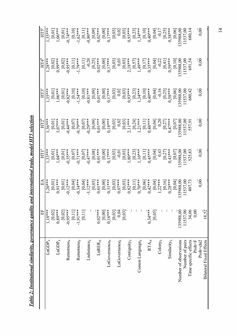
estimator as well as various sensitivity tests. Table 2 summarizes the main steps followed in
the estimation and the results of the appropriated statistical tests to justify the choice of this
�final� regression. It considers as endogenous the variables of GDP, distance, remoteness,
governance and real exchanges rate. My comments are based on this �final� regression
corrected of the selection bias (Table 1, column 2).
Concerning the traditional gravity variables, coefficients have the expected sign and are
significant at the 1% level. Exports volumes from i to j increase with GDP and parameters
estimates are close to unity as suggested by the theory. The elasticity of bilateral trade to
distance is -0.86 and the coefficients for the remoteness variables are significantly negative.
Sharing a common border raises bilateral exports by a factor 2.23 (e0.8), and speaking a
common language increase trade by 180% (e1.03-1). A common belonging to a preferential
trade agreement raises trade by a factor 1.4 (e0.36). Lastly, a real depreciation of the currency
of the exporting country leads to an increase of its exports.
Institutional similarity has a positive impact on bilateral exports. Indeed, its parameter
estimate is positive and significant at the 1% level. The fact that two countries share the same
institutional framework increases bilateral exports by 60% (e0.47-1).
The consequences of institutional quality on international trade are questionable, particularly
as far as the quality of governance in the importing country is concerned. Indeed, the
coefficient of the exporter quality of institution variable is positive and significant, indicating
that an increase in quality of governance in the exporting country raises bilateral trade. The
parameter estimate of the quality of governance in the importing country is also positive and
significant at the 10% threshold. But, the robustness checks (table 1 columns 3 and 4) shows
that this result is very sensitive to sample size variations. When the sample size is reduced the
coefficient of the importer governance is not significantly different of zero. Nevertheless,
coefficient estimates of the institutional similarity and of the exporter quality of governance
appear quite robust. Parameter estimates remain positive and highly significant.

13
Table 1: Institutional similarity, governance quality and international trade
1a 2b 3c 4d
LnGDPit 1,35*** 1,15*** 1,14*** 1,09***[0,01] [0,02] [0,02] [0,02]
LnGDPjt 1,06*** 0,86*** 0,86*** 0,84***[0,01] [0,02] [0,02] [0,02]
Remotnessit -0,74*** -0,91*** -0,91*** -1,01***[0,10] [0,10] [0,10] [0,09]
Remotnessjt -1,62*** -1,81*** -1,78*** -1,74***[0,11] [0,11] [0,10] [0,10]
Lndistanceij -0,80*** -0,86*** -0,83*** -0,78***[0,09] [0,09] [0,08] [0,09]
LnRERijt 0,02*** 0,02*** 0,02*** 0,02***[0,00] [0,00] [0,00] [0,00]
LnGovernanceit 0,17*** 0,19*** 0,18*** 0,10***[0,03] [0,03] [0,03] [0,02]
LnGovernancejt 0,02 0,05* 0,04 0,03[0,03] [0,03] [0,03] [0,02]
Contiguityij 0,93*** 0,80*** 0,82*** 1,12***[0,23] [0,22] [0,22] [0,23]
Comon languageij 1,34*** 1,03*** 1,04*** 1,08***[0,10] [0,10] [0,10] [0,10]
RTAijt 0,40*** 0,36*** 0,37*** 0,38***[0,04] [0,04] [0,04] [0,04]
Colonyij -0,17 -0,03 -0,03 -0,08[0,25] [0,24] [0,24] [0,24]
Similarityij 0,58*** 0,47*** 0,47*** 0,49***[0,06] [0,06] [0,06] [0,06]
PRESij _ 0,07*** 0,06*** 0,04***_ [0,01] [0,01] [0,01]
DDij _ 0,06 0,08 0,12_ [0,08] [0,08] [0,08]
PAijt _ 0,13*** 0,14*** 0,13***_ [0,02] [0,02] [0,02]
Number of observations 135988,00 135988,00 135600,00 129927,00Number of pairs 11537,00 11537,00 11511,00 11189,00
Time specific effects 680,14 690,51 697,78 756,69Prob>chi2 0,00 0,00 0,00 0,00
***, **, and * significant at the 1%, 5% and 10% levels respectively. Standard errors reported into brackets under coefficients. The time dummy variables and the constant are not reported to save space. a HT5 :endogenous variables: lnGDPit, lnGDPjt, lnDistanceij, lnGovernanceit, lnGovernancejt, remotnessit, remotnessjt et lnRERijt b HT5 : Addition of PRES, DD, PAt c ,d Values of the dependant variable that are respectively three and two standard deviations away from the mean are discarded.
14
Tabl
e 2:
Inst
itutio
nal s
imila
rity
, gov
erna
nce
qual
ity a
nd in
tern
atio
nal t
rade
, mod
el H
T5 se
lect
ion
EFEA
HT1
a H
T2b
HT3
cH
T4d
HT5
e Ln
GD
P it
1,18
***
1,20
***
1,33
***
1,36
***
1,35
***
1,28
***
1,35
***
[0
,02]
[0,0
1][0
,01]
[0
,01]
[0,0
1][0
,02]
[0,0
1]
LnG
DP j
t 0,
89**
*0,
91**
*1,
04**
* 1,
07**
*1,
06**
*0,
99**
*1,
06**
*
[0,0
2][0
,01]
[0,0
1]
[0,0
1][0
,01]
[0,0
2][0
,01]
R
emot
ness
it -0
,95*
**-0
,12*
**-0
,35*
**
-0,4
4***
-0,8
2***
-0,9
5***
-0,7
4***
[0,1
1][0
,04]
[0,0
7]
[0,0
7][0
,10]
[0,1
1][0
,10]
R
emot
ness
jt -1
,91*
**-0
,34*
**-0
,71*
**
-0,7
9***
-1,5
4***
-1,7
9***
-1,6
2***
[0,1
1][0
,04]
[0,0
7]
[0,0
7][0
,10]
[0,1
1][0
,11]
Ln
dist
ance
ij _
-1,1
2***
-0,4
7***
-0
,29*
**-0
,81*
**-0
,20
-0,8
0***
_[0
,03]
[0,0
8]
[0,0
9][0
,09]
[0,2
5][0
,09]
Ln
RER
ijt
0,02
***
0,01
***
0,01
***
0,01
***
0,01
***
0,02
***
0,02
***
[0
,00]
[0,0
0][0
,00]
[0
,00]
[0,0
0][0
,00]
[0,0
0]
LnG
over
nanc
e it
0,18
***
0,31
***
0,17
***
0,18
***
0,17
***
0,17
***
0,17
***
[0
,03]
[0,0
3][0
,03]
[0
,03]
[0,0
3][0
,03]
[0,0
3]
LnG
over
nanc
e jt
0,04
0,07
***
-0,0
1 0,
020,
020,
030,
02
[0
,03]
[0,0
3][0
,03]
[0
,03]
[0,0
3][0
,03]
[0,0
3]
Con
tigui
tyij
_0,
82**
*1,
80**
* 2,
11**
*0,
93**
*2,
18**
*0,
93**
*
_[0
,11]
[0,2
3]
[0,2
4][0
,23]
[0,5
7][0
,23]
C
omon
Lan
guag
e ij
_0,
70**
*1,
10**
* 1,
21**
*1,
34**
*1,
49**
*1,
34**
*
_[0
,06]
[0,1
1]
[0,1
1][0
,10]
[0,1
7][0
,10]
R
TAijt
0,
34**
*0,
42**
*0,
45**
* 0,
48**
*0,
40**
*0,
35**
*0,
40**
*
[0,0
5][0
,04]
[0,0
4]
[0,0
4][0
,04]
[0,0
4][0
,04]
C
olon
y ij
_1,
22**
*0,
43
0,20
-0,1
6-0
,22
-0,1
7
_[0
,16]
[0,2
7]
[0,2
7][0
,25]
[0,4
1][0
,25]
Si
mila
rity i
j _
0,28
***
0,43
***
0,47
***
0,58
***
0,59
***
0,58
***
_
[0,0
4][0
,07]
[0
,07]
[0,0
6][0
,10]
[0,0
6]
Num
ber o
f obs
erva
tions
13
5988
,00
1359
88,0
013
5988
,00
1359
88,0
013
5988
,00
1359
88,0
013
5988
,00
Num
ber o
f pai
rs
1153
7,00
1153
7,00
1153
7,00
11
537,
0011
537,
0011
537,
0011
537,
00
Tim
e sp
ecifi
c ef
fect
s 34
,06
407,
7352
5,83
55
7,91
680,
4269
1,54
680,
14
Prob
>F
0,00
__
__
__
Prob
>chi
2 _
0,00
0,00
0,
000,
000,
000,
00
Bila
tera
l Fix
ed E
ffec
ts
18,5
2_
_ _
__
_

15
Prob
>F
0,00
__
__
__
Hau
sman
test
fixe
d vs
rand
om e
ffec
tsf
_15
6,94
_ _
__
_ Pr
ob>c
hi2
_0,
00_
__
__
Hau
sman
HT
vs ra
ndom
eff
ects
g _
_53
8,62
56
5,23
270,
1525
,12
281,
79
Prob
>chi
2 _
_0,
00
0,00
0,00
0,00
0,00
Su
riden
tific
atio
n te
sth
__
303,
26
284,
8714
,16
0,00
0,00
Pr
ob>c
hi2
__
0,00
0,
000,
081,
001,
00
***,
**,
and
* si
gnifi
cant
at t
he 1
%, 5
% a
nd 1
0% le
vels
resp
ectiv
ely.
Sta
ndar
d er
rors
repo
rted
into
bra
cket
s und
er c
oeff
icie
nts.
The
time
dum
my
varia
bles
and
th
e co
nsta
nt a
re n
ot re
porte
d to
save
spac
e.
a HT1
:end
ogen
ous v
aria
bles
: lnG
DP i
t, ln
GD
P jt a
nd ln
Dist
ance
ij. b H
T2 :
endo
geno
us v
aria
bles
: lnG
DP i
t, ln
GD
P jt,
lnD
istan
ceij,
lnG
over
nanc
e it a
nd ln
gove
rnan
cejt
c HT3
: en
doge
nous
var
iabl
es: ln
GD
P it,
lnG
DP j
t, ln
Dist
ance
ij, ln
Gov
erna
nce it
, lnG
over
nanc
e jt, r
emot
ness
it et r
emot
ness
jt d H
T4 :
endo
geno
us v
aria
bles
: lnG
DP i
t, ln
GD
P jt,
lndi
stan
ceij,
lnG
over
nanc
e it, l
nGov
erna
nce jt
, rem
otne
ssit,
rem
otne
ssjt e
t RTA
ijt
e HT5
: en
doge
nous
var
iabl
es: ln
GD
P it,
lnG
DP j
t, ln
Dist
ance
ij, ln
Gov
erna
nce ij
t, ln
Gov
erna
nce jt
, rem
otne
ssit,
rem
otne
ssjt e
t lnR
ERijt
f Th
is te
st is
app
lied
to th
e di
ffer
ence
s bet
wee
n th
e fix
ed e
ffec
ts m
odel
and
the
rand
om e
ffec
ts m
odel
est
imat
es w
ithou
t tak
ing
into
acc
ount
the
coef
ficie
nt o
f tim
e ef
fect
s.
g H
auss
man
test
app
lied
to th
e di
ffer
ence
s bet
wee
n th
e ra
ndom
eff
ects
mod
el a
nd th
e H
T es
timat
ors,
with
out t
ime
effe
cts.
h Hau
sman
test
app
lied
to th
e di
ffer
ence
s bet
wee
n th
e fix
ed e
ffec
ts a
nd th
e H
T es
timat
ors,
with
out t
ime
effe
cts.
16
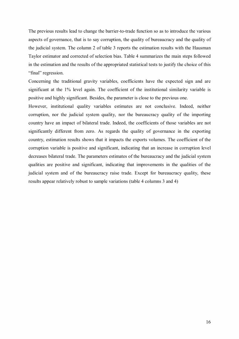
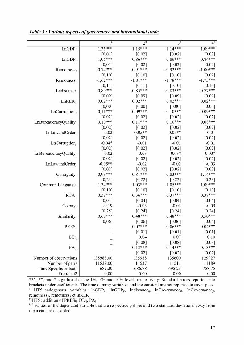
The previous results lead to change the barrier-to-trade function so as to introduce the various
aspects of governance, that is to say corruption, the quality of bureaucracy and the quality of
the judicial system. The column 2 of table 3 reports the estimation results with the Hausman
Taylor estimator and corrected of selection bias. Table 4 summarizes the main steps followed
in the estimation and the results of the appropriated statistical tests to justify the choice of this
�final� regression.
Concerning the traditional gravity variables, coefficients have the expected sign and are
significant at the 1% level again. The coefficient of the institutional similarity variable is
positive and highly significant. Besides, the parameter is close to the previous one.
However, institutional quality variables estimates are not conclusive. Indeed, neither
corruption, nor the judicial system quality, nor the bureaucracy quality of the importing
country have an impact of bilateral trade. Indeed, the coefficients of those variables are not
significantly different from zero. As regards the quality of governance in the exporting
country, estimation results shows that it impacts the exports volumes. The coefficient of the
corruption variable is positive and significant, indicating that an increase in corruption level
decreases bilateral trade. The parameters estimates of the bureaucracy and the judicial system
qualities are positive and significant, indicating that improvements in the qualities of the
judicial system and of the bureaucracy raise trade. Except for bureaucracy quality, these
results appear relatively robust to sample variations (table 4 columns 3 and 4)
17
Table 3 : Various aspects of governance and international trade
1a 2b 3c 4d
LnGDPit 1,35*** 1.15*** 1.14*** 1.09*** [0,01] [0.02] [0.02] [0.02]
LnGDPjt 1,06*** 0.86*** 0.86*** 0.84*** [0,01] [0.02] [0.02] [0.02]
Remotnessit -0,74*** -0.91*** -0.92*** -1.00*** [0,10] [0.10] [0.10] [0.09]
Remotnessjt -1,62*** -1.81*** -1.78*** -1.73*** [0,11] [0.11] [0.10] [0.10]
Lndistanceij -0,80*** -0.85*** -0.83*** -0.77*** [0,09] [0.09] [0.09] [0.09]
LnRERijt 0,02*** 0.02*** 0.02*** 0.02*** [0,00] [0.00] [0.00] [0.00]
LnCorruptionit -0,11*** -0.09*** -0.10*** -0.09*** [0,02] [0.02] [0.02] [0.02]
LnBureaucracyQualityit 0,10*** 0.11*** 0.10*** 0.08*** [0,02] [0.02] [0.02] [0.02]
LnLawandOrderit 0,02 0.05** 0.05** 0.01 [0,02] [0.02] [0.02] [0.02]
LnCorruptionjt -0,04* -0.01 -0.01 -0.01 [0,02] [0.02] [0.02] [0.02]
LnBureaucracyQualityjt 0,02 0.03 0.03* 0.03* [0,02] [0.02] [0.02] [0.02]
LnLawandOrderjt -0,05** -0.02 -0.02 -0.03 [0,02] [0.02] [0.02] [0.02]
Contiguityij 0,93*** 0.81*** 0.83*** 1.14*** [0,23] [0.22] [0.22] [0.23]
Common Languageij 1,34*** 1.03*** 1.05*** 1.09*** [0,10] [0.10] [0.10] [0.10]
RTAijt 0,39*** 0.36*** 0.37*** 0.37*** [0,04] [0.04] [0.04] [0.04]
Colonyij -0,19 -0.03 -0.03 -0.09 [0,25] [0.24] [0.24] [0.24]
Similarityij 0,60*** 0.48*** 0.48*** 0.50*** [0,06] [0.06] [0.06] [0.06]
PRESij _ 0.07*** 0.06*** 0.04*** _ [0.01] [0.01] [0.01]
DDij _ 0.04 0.07 0.10 _ [0.08] [0.08] [0.08]
PAijt _ 0.13*** 0.14*** 0.13*** _ [0.02] [0.02] [0.02]
Number of observations 135988,00 135988 135600 129927Number of pairs 11537,00 11537 11511 11189
Time Specific Effects 682,20 686.78 695.23 758.75Prob>chi2 0,00 0.00 0.00 0.00
***, **, and * significant at the 1%, 5% and 10% levels respectively. Standard errors reported into brackets under coefficients. The time dummy variables and the constant are not reported to save space. a HT5 :endogenous variables: lnGDPit, lnGDPjt, lndistanceij, lnGovernanceit, lnGovernancejt, remotnessit, remotnessjt et lnRERijt b HT5 : addition of PRESij, DDij, PAijt c, d Values of the dependant variable that are respectively three and two standard deviations away from the mean are discarded.

18
Tabl
e 4:
Var
ious
asp
ects
of g
over
nanc
e an
d in
tern
atio
nal t
rade
, mod
el H
T5 se
lect
ion
EF
EAH
T1a
HT2
bH
T3c
HT4
dH
T5e
LnG
DP i
t 1,
18**
*1,
19**
*1,
32**
* 1,
36**
*1,
35**
*1,
28**
*1,
35**
* [0
,02]
[0,0
1][0
,01]
[0
,02]
[0,0
1][0
,02]
[0,0
1]
LnG
DP j
t 0,
89**
*0,
91**
*1,
03**
* 1,
07**
*1,
06**
*0,
99**
*1,
06**
* [0
,02]
[0,0
1][0
,01]
[0
,02]
[0,0
1][0
,02]
[0,0
1]
Rem
otne
ssit
-0,9
5***
-0,0
9**
-0,3
1***
-0
,42*
**-0
,81*
**-0
,95*
**-0
,74*
**
[0,1
1][0
,04]
[0,0
7]
[0,0
7][0
,10]
[0,1
1][0
,10]
R
emot
ness
jt -1
,92*
**-0
,35*
**-0
,72*
**
-0,8
1***
-1,5
6***
-1,8
0***
-1,6
2***
[0
,11]
[0,0
4][0
,07]
[0
,07]
[0,1
0][0
,11]
[0,1
1]
Lndi
stan
ceij
_-1
,12*
**-0
,54*
**
-0,2
8***
-0,8
0***
-0,1
7-0
,80*
**
_[0
,03]
[0,0
8]
[0,0
9][0
,09]
[0,2
5][0
,09]
Ln
RER
ijt
0,02
***
0,01
***
0,01
***
0,01
***
0,01
***
0,01
***
0,02
***
[0,0
0][0
,00]
[0,0
0]
[0,0
0][0
,00]
[0,0
0][0
,00]
Ln
Cor
rupt
ion it
-0
,09*
**-0
,11*
**-0
,10*
**
-0,1
1***
-0,1
2***
-0,1
1***
-0,1
1***
[0
,02]
[0,0
2][0
,02]
[0
,02]
[0,0
2][0
,02]
[0,0
2]
LnBu
reau
crac
yQua
lity it
0,
10**
*0,
15**
*0,
10**
* 0,
10**
*0,
10**
*0,
10**
*0,
10**
* [0
,02]
[0,0
2][0
,02]
[0
,02]
[0,0
2][0
,02]
[0,0
2]
LnLa
wan
dOrd
erit
0,05
**0,
09**
*0,
04
0,03
0,02
0,03
0,02
[0
,02]
[0,0
2][0
,02]
[0
,02]
[0,0
2][0
,02]
[0,0
2]
LnC
orru
ptio
n jt
-0,0
20,
010,
00
-0,0
2-0
,03
-0,0
3-0
,04*
[0
,02]
[0,0
2][0
,02]
[0
,02]
[0,0
2][0
,02]
[0,0
2]
LnBu
reau
crac
yQua
lity jt
0,
030,
05**
*0,
01
0,02
0,02
0,02
0,02
[0
,02]
[0,0
2][0
,02]
[0
,02]
[0,0
2][0
,02]
[0,0
2]
LnLa
wan
dOrd
erjt
-0,0
2-0
,01
-0,0
5**
-0,0
5**
-0,0
6**
-0,0
4*-0
,05*
* [0
,02]
[0,0
2][0
,02]
[0
,02]
[0,0
2][0
,02]
[0,0
2]
Con
tigui
tyij
_0,
83**
*1,
68**
* 2,
13**
*0,
93**
*2,
24**
*0,
93**
* _
[0,1
1][0
,23]
[0
,24]
[0,2
3][0
,56]
[0,2
3]
Com
mon
Lan
guag
e ij
_0,
70**
*1,
07**
* 1,
21**
*1,
34**
*1,
50**
*1,
34**
* _
[0,0
6][0
,11]
[0
,11]
[0,1
0][0
,17]
[0,1
0]
RTA
ijt
0,33
***
0,41
***
0,44
***
0,47
***
0,39
***
0,35
***
0,39
***
[0,0
5][0
,04]
[0,0
4]
[0,0
4][0
,04]
[0,0
4][0
,04]
C
olon
y ij
_1,
21**
*0,
46*
0,18
-0,1
9-0
,26
-0,1
9 _
[0,1
6][0
,27]
[0
,27]
[0,2
5][0
,40]
[0,2
5]

19
Sim
ilarit
y ij
_0,
28**
*0,
43**
* 0,
48**
*0,
60**
*0,
61**
*0,
60**
* _
[0,0
4][0
,06]
[0
,07]
[0,0
6][0
,10]
[0,0
6]
Num
ber o
f obs
erva
tions
1359
88,0
013
5988
,00
1359
88,0
0 13
5988
,00
1359
88,0
013
5988
,00
1359
88,0
0 N
umbe
r of p
airs
1153
7,00
1153
7,00
1153
7,00
11
537,
0011
537,
0011
537,
0011
537,
00
Tim
e Sp
ecifi
c Ef
fect
s33
,97
403,
3651
8,36
55
6,63
682,
4769
5,19
682,
20
Prob
>F0,
00_
_ _
__
_ Pr
ob>c
hi2
_0,
000,
00
0,00
0,00
0,00
0,00
Bi
late
ral F
ixed
Eff
ects
18
,44
__
__
__
Prob
>F0,
00_
_ _
__
_ H
ausm
an te
st fi
xed
vs ra
ndom
eff
ects
f_
185,
47_
__
__
Prob
>chi
2_
0,00
_ _
__
_ H
ausm
an H
T vs
rand
om e
ffec
tsg
__
497,
32
2456
,70
261,
9122
,07
265,
42
Prob
>chi
2_
_0,
00
0,00
0,00
0,00
0,00
Su
riden
tific
atio
n te
sth
__
251,
95
273,
3911
,26
0,00
0,00
Pr
ob>c
hi2
__
0,00
0,
000,
511,
001,
00
***,
**,
and
* si
gnifi
cant
at t
he 1
%, 5
% a
nd 1
0% le
vels
resp
ectiv
ely.
Sta
ndar
d er
rors
repo
rted
into
bra
cket
s und
er c
oeff
icie
nts.
The
time
dum
my
varia
bles
and
th
e co
nsta
nt a
re n
ot re
porte
d to
save
spac
e.
a HT1
:end
ogen
ous v
aria
bles
: lnG
DP i
t, ln
GD
P jt a
nd ln
Dist
ance
ij. b H
T2 :
endo
geno
us v
aria
bles
: lnG
DP i
t, ln
GD
P jt,
lnD
istan
ceij,
lnC
orru
ptio
n it, l
nBur
eauc
racy
Qua
lity it
, lnL
awan
dOrd
erit,
lnC
orru
ptio
n jt, l
nBur
eauc
racy
Qua
lity j
t, an
d ln
Law
andO
rder
jt. c H
T3 :
endo
geno
us v
aria
bles
: lnG
DP i
t, ln
GD
P jt,
lnD
istan
ceij,
lnC
orru
ptio
n it, l
nBur
eauc
racy
Qua
lity it
, lnL
awan
dOrd
erit,
lnC
orru
ptio
n jt, l
nBur
eauc
racy
Qua
lity j
t, ln
Law
andO
rder
jt, re
mot
ness
it and
rem
otne
ssjt
d HT4
: en
doge
nous
var
iabl
es: ln
GD
P it,
lnG
DP j
t, ln
dist
ance
ij, ln
GD
P it,
lnG
DP j
t, ln
Dist
ance
ij, ln
Cor
rupt
ion it
, lnB
urea
ucra
cyQ
ualit
y it, l
nLaw
andO
rder
it, ln
Cor
rupt
ion jt
, lnB
urea
ucra
cyQ
ualit
y jt, l
nLaw
andO
rder
jt,, re
mot
ness
it, re
mot
ness
jt and
RTA
ijt
e HT5
: en
doge
nous
var
iabl
es: ln
GD
P it,
lnG
DP j
t, ln
Dist
ance
ij, ln
GD
P it,
lnG
DP j
t, ln
Dist
ance
ij, ln
Cor
rupt
ion it
, lnB
urea
ucra
cyQ
ualit
y it, l
nLaw
andO
rder
it, ln
Cor
rupt
ion jt
, lnB
urea
ucra
cyQ
ualit
y jt, l
nLaw
andO
rder
jt, re
mot
ness
it, re
mot
ness
jt and
lnR
ERijt
f Th
is te
st is
app
lied
to th
e di
ffer
ence
s bet
wee
n th
e fix
ed e
ffec
ts m
odel
and
the
rand
om e
ffec
ts m
odel
est
imat
es w
ithou
t tak
ing
into
acc
ount
the
coef
ficie
nt o
f tim
e ef
fect
s.
g H
auss
man
test
app
lied
to th
e di
ffer
ence
s bet
wee
n th
e ra
ndom
eff
ects
mod
el a
nd th
e H
T es
timat
ors,
with
out t
ime
effe
cts.
h Hau
sman
test
app
lied
to th
e di
ffer
ence
s bet
wee
n th
e fix
ed e
ffec
ts a
nd th
e H
T es
timat
ors,
with
out t
ime
effe
cts.

20
These first results clearly show that institutional similarity noticeably eases bilateral exports. Indeed,
the fact that two countries share the same institutional framework increases bilateral exports
by 60% (e0.47-1).
These results do not confirm Anderson & Marcouiller�s view according to which bad
governance is a barrier to trade. Institutional quality seems to play a more complex part in
international trade. Indeed, the estimations show that the quality of governance of the
exporting country matters for trade, on the contrary of the one of the importing country.
These first results lead to change the barrier-to-trade function in order to take into account the
interactions between the different aspects of governance. This new formulation of the barrier-
to-trade function enables to test the �second best� theories that see corruption as a way to
grease the wheels of commerce.
V DOES CORRUPTION �GREASE THE WHEELS� OF COMMERCE?
�Second best� theories consider corruption as a way to �grease� the wheels of commerce,
because it compensates the consequences of a defective bureaucracy or bad policies. Testing
empirically these theories requires a measure of these distortions. The Fraser institute
Economic Freedom index seems the more appropriate. Indeed, it measures the degree to
which the policies and institutions of countries are supportive of economic freedom, that is to
say personal choice, voluntary exchange, freedom to compete, and security of privately
owned property. However, that indicator because has been produced yearly only since the
year 2000. That is why; I prefer using the IRCG rating on bureaucracy quality.
Remind that, the �second best� theories will be confirmed, if the coefficients of corruption
variables are positive and the ones of interactions variables negative.
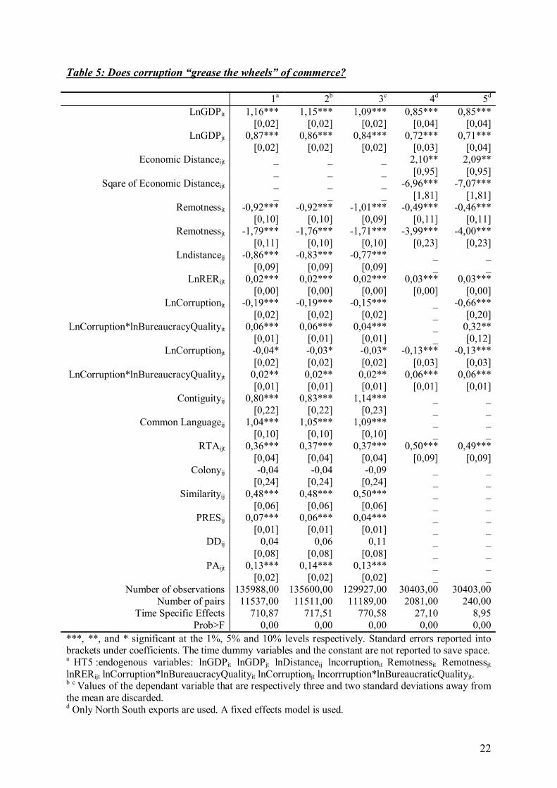
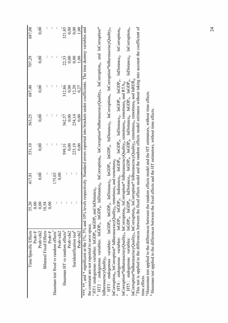
The first column of Table 5 reports the estimation of equation (11) with the Hausman Taylor
estimator and corrected of a selection bias. Table 6 explains the choice of the endogenous
variables. Again, coefficients of the traditional gravity variables have the expected sign and
are significant at the 1% level again. Again, institutional similarity has a positive and
significant impact on exports volumes.
As regard the variables of interest, the coefficients of the corruption variables are negative and
significant at the 1% level for the exporting country and at 10% one for the importing
country. Moreover, parameters estimates of the interaction variables are positives and highly

21
significant. Hence, these estimation results invalidate totally the predictions of �second best�
theories. They show that corruption in the importing country as well as in the exporting
country is a barrier to bilateral exports, and that it is even more harmful to trade when the
quality of bureaucracy is weak.
The columns 2 and 3 of table 5 present estimations of HT5 on samples where extreme values
of the dependant variable have been discarded. The sign and the significance level of
coefficients of the variables of interest are not change by these sample variations.
Since corruption can lead to fallacious data on international trade, equation (11) is estimated
on a sample made of Northern countries as exporters8, and Southern countries as importers.
Indeed, widespread corruption and poor governance seem to be an issue specific to southern
countries. As economic distance could have an ambiguous effect on North South trade, I add
to the traditional gravity equation a relative economic distance index9 and it square. Indeed,
on the one hand, it captures distance in standard of living likely to decrease trade of
horizontally differentiated goods. On the other hand, it reflects differences in capitalistic
intensities which favour inter industry trade linked to differences in factor endowments.
Estimations of equation (11) on a North South sample are reported in columns (4) and (5) of
table (5). In those estimations, the bilateral specific effects are treated as fixed because I
failed to obtain sufficiently strong instruments among the set of explanatory variables to
apply a Hausman Taylor estimator. Again, the gravity equation performs well. The
coefficients have the expected signs. For instance, GDP increases trade whereas remoteness
reduces it. The existence of a non linear effect for economic distance is confirmed. Indeed,
difference in standard of living appears as a good proxy both for similarity of supply and
demand structures, and for distance in capitalistic intensities. As regard the variables of
interest, estimations show again that corruption in the importing country as well as in the
exporting country is a barrier to bilateral exports, and that it is even more harmful to trade
when the quality of bureaucracy is weak.
8 Northern countries correspond to the 22 high income OECD countries and Southern countries to 122 developing countries. I adopt a broad definition of South since I group together countries belonging to Eastern Europe, Middle East, Latin America or Sub Saharan Africa. 9 1 It is calculated from a formula inspired by Balassa and Bauwens (1987) which gives an index contained between 0 (standard of living equality) and 1 (maximal difference in standard of living):
2ln2)z2ln()z2(zlnzdeco −−+= with
=
jty;ityMax
jty;ityMinz where yit and yjt are respectively the real
income per capita of the exporter and of the importer at time t.
22
Table 5: Does corruption �grease the wheels� of commerce?
1a 2b 3c 4d 5d
LnGDPit 1,16*** 1,15*** 1,09*** 0,85*** 0,85*** [0,02] [0,02] [0,02] [0,04] [0,04]
LnGDPjt 0,87*** 0,86*** 0,84*** 0,72*** 0,71*** [0,02] [0,02] [0,02] [0,03] [0,04]
Economic Distanceijt _ _ _ 2,10** 2,09** _ _ _ [0,95] [0,95]
Sqare of Economic Distanceijt _ _ _ -6,96*** -7,07*** _ _ _ [1,81] [1,81]
Remotnessit -0,92*** -0,92*** -1,01*** -0,49*** -0,46*** [0,10] [0,10] [0,09] [0,11] [0,11]
Remotnessjt -1,79*** -1,76*** -1,71*** -3,99*** -4,00*** [0,11] [0,10] [0,10] [0,23] [0,23]
Lndistanceij -0,86*** -0,83*** -0,77*** _ _ [0,09] [0,09] [0,09] _ _
LnRERijt 0,02*** 0,02*** 0,02*** 0,03*** 0,03*** [0,00] [0,00] [0,00] [0,00] [0,00]
LnCorruptionit -0,19*** -0,19*** -0,15*** _ -0,66*** [0,02] [0,02] [0,02] _ [0,20]
LnCorruption*lnBureaucracyQualityit 0,06*** 0,06*** 0,04*** _ 0,32** [0,01] [0,01] [0,01] _ [0,12]
LnCorruptionjt -0,04* -0,03* -0,03* -0,13*** -0,13*** [0,02] [0,02] [0,02] [0,03] [0,03]
LnCorruption*lnBureaucracyQualityjt 0,02** 0,02** 0,02** 0,06*** 0,06*** [0,01] [0,01] [0,01] [0,01] [0,01]
Contiguityij 0,80*** 0,83*** 1,14*** _ _ [0,22] [0,22] [0,23] _ _
Common Languageij 1,04*** 1,05*** 1,09*** _ _ [0,10] [0,10] [0,10] _ _
RTAijt 0,36*** 0,37*** 0,37*** 0,50*** 0,49*** [0,04] [0,04] [0,04] [0,09] [0,09]
Colonyij -0,04 -0,04 -0,09 _ _ [0,24] [0,24] [0,24] _ _
Similarityij 0,48*** 0,48*** 0,50*** _ _ [0,06] [0,06] [0,06] _ _
PRESij 0,07*** 0,06*** 0,04*** _ _ [0,01] [0,01] [0,01] _ _
DDij 0,04 0,06 0,11 _ _ [0,08] [0,08] [0,08] _ _
PAijt 0,13*** 0,14*** 0,13*** _ _ [0,02] [0,02] [0,02] _ _
Number of observations 135988,00 135600,00 129927,00 30403,00 30403,00Number of pairs 11537,00 11511,00 11189,00 2081,00 240,00
Time Specific Effects 710,87 717,51 770,58 27,10 8,95Prob>F 0,00 0,00 0,00 0,00 0,00
***, **, and * significant at the 1%, 5% and 10% levels respectively. Standard errors reported into brackets under coefficients. The time dummy variables and the constant are not reported to save space. a HT5 :endogenous variables: lnGDPit lnGDPjt lnDistanceij lncorruptionit Remotnessit Remotnessjt lnRERijt lnCorruption*lnBureaucracyQualityit lnCorruptionjt lncorrruption*lnBureaucraticQualityjt. b c Values of the dependant variable that are respectively three and two standard deviations away from the mean are discarded. d Only North South exports are used. A fixed effects model is used.

23
Tabl
e 6:
Doe
s cor
rupt
ion
�gre
ase
the
whe
els�
of c
omm
erce
? H
T5 m
odel
sele
ctio
n
EF
EAH
T1a
HT2
bH
T3c
HT4
dH
T5e
LnG
DPi
t 1,
19**
*1,
20**
*1,
33**
* 1,
36**
*1,
35**
*1,
29**
*1,
35**
*
[0,0
2][0
,01]
[0,0
1]
[0,0
1][0
,01]
[0,0
2][0
,01]
Ln
GD
Pjt
0,90
***
0,91
***
1,03
***
1,07
***
1,06
***
1,00
***
1,06
***
[0
,02]
[0,0
1][0
,01]
[0
,01]
[0,0
1][0
,02]
[0,0
1]
Rem
otne
ssit
-0
,96*
**-0
,12*
**-0
,33*
**
-0,4
3***
-0,8
3***
-0,9
6***
-0,7
5***
[0,1
1][0
,04]
[0,0
7]
[0,0
7][0
,10]
[0,1
1][0
,10]
R
emot
ness
jt
-1,9
0***
-0,3
5***
-0,7
1***
-0
,80*
**-1
,53*
**-1
,78*
**-1
,61*
**
[0
,11]
[0,0
4][0
,07]
[0
,07]
[0,1
0][0
,11]
[0,1
1]
LnD
istan
ceij
_
-1,1
2***
-0,5
2***
-0
,28*
**-0
,80*
**-0
,18
-0,8
0***
_[0
,03]
[0,0
8]
[0,0
9][0
,09]
[0,2
5][0
,09]
Ln
RER
ijt
0,02
***
0,01
***
0,01
***
0,01
***
0,01
***
0,01
***
0,02
***
[0
,00]
[0,0
0][0
,00]
[0
,00]
[0,0
0][0
,00]
[0,0
0]
LnC
orru
ptio
nit
-0,1
9***
-0,2
6***
-0,1
9***
-0
,19*
**-0
,20*
**-0
,19*
**-0
,19*
**
[0
,02]
[0,0
2][0
,02]
[0
,02]
[0,0
2][0
,02]
[0,0
2]
LnC
orru
ptio
n*ln
Bure
aucr
acyQ
ualit
yit
0,06
***
0,09
***
0,06
***
0,06
***
0,05
***
0,05
***
0,05
***
[0
,01]
[0,0
1][0
,01]
[0
,01]
[0,0
1][0
,01]
[0,0
1]
LnC
orru
ptio
njt
-0,0
4*-0
,04*
*0,
00
-0,0
3-0
,03
-0,0
4*-0
,04*
[0,0
2][0
,02]
[0,0
2]
[0,0
2][0
,02]
[0,0
2][0
,02]
Ln
Cor
rupt
ion*
lnBu
reau
crac
yQua
lityj
t 0,
02*
0,04
***
0,02
0,
02*
0,01
0,02
0,01
[0,0
1][0
,01]
[0,0
1]
[0,0
1][0
,01]
[0,0
1][0
,01]
C
ontig
uity
ij
_0,
82**
*1,
71**
* 2,
13**
*0,
93**
*2,
23**
*0,
93**
*
_[0
,11]
[0,2
3]
[0,2
4][0
,23]
[0,5
6][0
,23]
C
omm
on L
angu
agei
j _
0,70
***
1,09
***
1,21
***
1,34
***
1,50
***
1,34
***
_
[0,0
6][0
,11]
[0
,11]
[0,1
0][0
,17]
[0,1
0]
RTA
ijt
0,33
***
0,41
***
0,45
***
0,47
***
0,40
***
0,35
***
0,40
***
[0
,05]
[0,0
4][0
,04]
[0
,04]
[0,0
4][0
,04]
[0,0
4]
Col
onyi
j _
1,21
***
0,43
0,
19-0
,18
-0,2
6-0
,19
_
[0,1
6][0
,27]
[0
,27]
[0,2
5][0
,40]
[0,2
5]
Sim
ilarit
yij
_0,
28**
*0,
43**
* 0,
48**
*0,
59**
*0,
61**
*0,
59**
*
_[0
,04]
[0,0
7]
[0,0
7][0
,06]
[0,1
0][0
,06]
N
umbe
r of o
bser
vatio
ns
1359
88,0
013
5988
,00
1359
88,0
0 13
5988
,00
1359
88,0
013
5988
,00
1359
88,0
0 N
umbe
r of p
airs
11
537,
0011
537,
0011
537,
00
1153
7,00
1153
7,00
1153
7,00
1153
7,00
24
Tim
e Sp
ecifi
c Ef
fect
s 35
,20
417,
8153
1,10
56
3,25
687,
4070
7,29
687,
08
Prob
>F
0,00
__
__
__
Prob
>chi
2 0,
000,
000,
00
0,00
0,00
0,00
0,00
Bi
late
ral F
ixed
Eff
ects
18
,58
__
__
__
Prob
>F
0,00
__
__
__
Hau
sman
test
fixe
d vs
rand
om e
ffec
tsf
_17
5,03
_ _
__
_ Pr
ob>c
hi2
_0,
00_
__
__
Hau
sman
HT
vs ra
ndom
eff
ects
g _
_59
9,31
56
2,57
312,
8622
,33
321,
85
Prob
>chi
2 _
_0,
00
0,00
0,00
0,00
0,00
Su
riden
tific
atio
n te
sth
__
223,
19
254,
1412
,20
0,00
0,00
Pr
ob>c
hi2
__
0,00
0,
000,
271,
001,
00
***,
**,
and
* si
gnifi
cant
at t
he 1
%, 5
% a
nd 1
0% le
vels
resp
ectiv
ely.
Sta
ndar
d er
rors
repo
rted
into
bra
cket
s und
er c
oeff
icie
nts.
The
time
dum
my
varia
bles
and
th
e co
nsta
nt a
re n
ot re
porte
d to
save
spac
e.
a HT1
:end
ogen
ous v
aria
bles
: lnG
DP i
t, ln
GD
P jt a
nd ln
Dist
ance
ij. b H
T2 :
end
ogen
ous
varia
bles
: ln
GD
P it,
lnG
DP j
t, ln
Dist
ance
ij, ln
Cor
rupt
ion it
, ln
Cor
rupt
ion*
lnBu
reau
crac
yQua
lity it
, ln
Cor
rupt
ion j
t, an
d ln
Cor
rupt
ion*
ln
Bure
aucr
acyQ
ualit
y jt.
c H
T3 :
endo
geno
us
varia
bles
:
lnG
DP i
t, ln
GD
P jt,
lnD
istan
ceij,
lnG
DP i
t, ln
GD
P jt,
lnD
istan
ceij,
lnC
orru
ptio
n it,
lnC
orru
ptio
n*ln
Bure
aucr
acyQ
ualit
y it,
lnC
orru
ptio
n jt, l
nCor
rupt
ion*
lnBu
reau
crac
yQua
lity jt
, rem
otne
ssit a
nd re
mot
ness
jt d
HT4
: en
doge
nous
va
riabl
es:
ln
GD
P it,
lnG
DP j
t, ln
dist
ance
ij, ln
GD
P it,
lnG
DP j
t, ln
Dist
ance
ij, ln
GD
P it,
lnG
DP j
t, ln
Dist
ance
ij, ln
Cor
rupt
ion it
, ln
Cor
rupt
ion*
lnBu
reau
crac
yQua
lity i
t, ln
Cor
rupt
ion jt
, lnC
orru
ptio
n* ln
Bure
aucr
acyQ
ualit
y jt, r
emot
ness
it, re
mot
ness
jt and
RTA
ijt
e H
T5 :
endo
geno
us
varia
bles
:
lnG
DP i
t, ln
GD
P jt,
lnD
istan
ceij,
lnG
DP i
t, ln
GD
P jt,
lnD
istan
ceij,
lnG
DP i
t, ln
GD
P jt,
lnD
istan
ceij,
lnC
orru
ptio
n it,
lnC
orru
ptio
n*ln
Bure
aucr
acyQ
ualit
y it,
lnC
orru
ptio
n jt, l
nCor
rupt
ion*
lnBu
reau
crac
yQua
lity jt
, rem
otne
ssit,
rem
otne
ssjt a
nd ln
RER
ijt
f This
test
is a
pplie
d to
the
diff
eren
ces
betw
een
the
fixed
eff
ects
mod
el a
nd th
e ra
ndom
eff
ects
mod
el e
stim
ates
with
out t
akin
g in
to a
ccou
nt th
e co
effic
ient
of
time
effe
cts.
g H
auss
man
test
app
lied
to th
e di
ffer
ence
s bet
wee
n th
e ra
ndom
eff
ects
mod
el a
nd th
e H
T es
timat
ors,
with
out t
ime
effe
cts.
h Hau
sman
test
app
lied
to th
e di
ffer
ence
s bet
wee
n th
e fix
ed e
ffec
ts a
nd th
e H
T es
timat
ors,
with
out t
ime
effe
cts.

25
VI CONCLUSION
Estimations clearly show that institutional similarity eases bilateral trade. The fact that two
countries have the same institutional framework increases export volumes by 60%.
Nevertheless, the consequences on international trade appear to be more complex than what
has suggested a recent literature. My results do not confirm either �second best� theories that
see corruption is a way to bypass rigidities imposed by governments. Thank to a barrier to
trade function which enables interaction between corruption and other aspects of governance,
this paper shows that corruption in the importing country as well as in the exporting country is
a barrier to bilateral exports, and that it is even more harmful to trade when the quality of
bureaucracy is weak. In a North-South approach, testing the impact of corruption and poor
governance on the exports of various types of goods and especially capital goods appears of
great interest because for developing countries exports from industrialised ones are a way to
acquire new goods.
References :
Anderson, J.E. & Marcouiller, D. (2002) �Insecurity and the pattern of trade : an empirical investigation�. The Review of Economics and Statistics, 84, 2, 342-52.
Anderson, J.E. & van Wincoop, E. (2003) �Gravity with Gravitas: A Solution to the Border Puzzle�. American Economic Review, 93, 1, 170�92.
Anderson, J. E., & van Wincoop, E. (2004) �Trade Costs�. Journal of Economic Literature, forthcoming.
Anderson, J. E., & Young, L. (1999) �Trade and Contract Enforcement�. Boston College Mimeograph.
Baghwati, J. N. (1982) �Directly Unproductive, Profit-seeking Activities� Journal of Political Economy, 90, 5, 988-1002.
Balassa, B. & Bauwens, L. (1987) �Intra-Industry Specialization in a Multi-Country and Multilateral Framework�. The Economic Journal, 97, 923-39.
Bayoumi, T. & Eichengreen, B. (1997) �Is regionalism simply a diversion? Evidence from the evolution the EC and the EFTA�. In: Ito, T., Krueger, A. (Eds.), Regionalism Versus Multilateral Trade Arrangements, Vol.6, Chapter 6. University of Chicago Press, Chicago.
Chong, A. & Zanforlin, L. (2000) �Law Tradition and Institutional Quality: Some Empirical Evidence�. Journal of International Development, 12, 8, 1057-68.
Carrere, C. (2004) �Revisiting the effects of regional trading agreements on trade flows with proper specification of the gravity model�. European Economic Review, forthcoming.
Disdier, A-C & Mayer, T. (2005) �Je t�aime, moi non plus: bilateral opinion and international trade� CEPR Discussion Paper No:4928.
Egger, P. (2000) �A note on the proper specification of the gravity equation�. Economics Letters, 66, 1, 25-31.
Egger, P (2002) �An econometric view on the estimation of gravity models and the calculations of trade potentials�. The World Economy, 25, 2, 297-312.

26
Egger, P. and Pfaffermayr, M. (2003) �The proper econometric specification of the gravity equation: A three way model with bilateral interaction effects�. Empirical Economics, 28, 3, pp.571-81.
Feenstra, R. (2004) Advanced International Trade: Theory and Evidence, Princeton: Princeton University Press.
Guillotin, Y. & Sevestre, P. (1994) �Estimations de fonctions de gains sur données de panel: Endogeneité du capital humain et effets de sélection�. Economie et Prévision 116, 119-135
Hausman, A. & Taylor, E. (1981) �Panel data and unobservable individuals effects�. Econometrica 49, 1377-1398.
Knack, S. & Keefer, P. (1995) �Institutions and Economic Performance: Cross-Country Tests Using Alternative Institutional Measures�. Economics and Politics, 7, 3, 207-27.
Nijman, T. & Verbeek, M. (1992) �Incomplete panels and selection bias� In: Matyas, L., Sevestre, P.(Eds), The Econometrics of Panel Data. Kluwer, Dordrecht, pp 262-302.
Rose, A.K. (2000) �One Money One Market: The Effect of Common Currencies on Trade�. Economic Policy, 30, 9�45.
Soloaga, I. & Winters, A. (2001) �How has regionalism in the 1990�s affected trade? North American Journal of Economics and Finance 12, 1-29.
Watson, A. (1974). Legal Transplants. Charlottesville, VA: University of Virginia Press.
Wei, S.J. (1996) �Intra-National Versus International Trade: How Stubborn are Nations in Global Integration?� NBER Working Paper, No. 5531 (Cambridge, MA: NBER).
ANNEXE 1: LIST OF COUNTRIES IN THE SAMPLE. Albania Ecuador Lebanon Spain Algeria Egypt Lithuania Sri Lanka Angola El Salvador Macedonia, FYR Sudan Argentina Equatorial Guinea Madagascar Sweden Australia Estonia Malawi Switzerland Austria Ethiopia Malaysia Syrian Arab Republic Azerbaijan Fiji Mali Tajikistan Bahamas, The Finland Malta Tanzania Bahrain, Kingdom of France Mauritania Thailand Bangladesh Gabon Mauritius Togo Barbados Gambia, The Mexico Trinidad and Tobago Belarus Georgia Moldova Tunisia Belgium Germany Mongolia Turkey Belize Ghana Morocco Turkmenistan Benin Greece Nepal Uganda Bolivia Grenada Netherlands Ukraine Brazil Guatemala New Zealand United Kingdom Bulgaria Guinea Niger United States Burkina Faso Guinea-Bissau Nigeria Uruguay Burundi Guyana Norway Uzbekistan Cambodia Haiti Oman Venezuela, Rep Bol Cameroon Honduras Panama Vietnam Canada Hungary Papua New Guinea Yugoslavia, SFR Cape Verde Iceland Paraguay Zambia Central African Rep India Peru Zimbabwe Chad Indonesia Philippines Chile Iran, IR of Poland China,PR: Mainland Ireland Portugal

27
Colombia Israel Romania Congo, Dem Rep of Italy Russia Congo, Republic of Jamaica Rwanda Costa Rica Japan Samoa Côte d'Ivoire Jordan Saudi Arabia Croatia Kazakhstan Senegal Cyprus Kenya Sierra Leone Czech Republic Korea Singapore Denmark Kuwait Slovak Republic Djibouti Kyrgyz Republic Slovenia Dominica Lao People's DemRep South Africa Dominican Republic Latvia
ANNEXE 2 : VARIABLES DESCRIPTION. Variable Name: Bilateral exports (Xij) Description: Bilateral exports of the country i to the country j, in F.O.B terms and in U.S. $ deflated by the American Consumer Price Index (1995=100), years 1984-1997. Source: IMF, Direction of Trade Statistics. Variable Name: GDPi(j) Description: Total Gross Domestic Product in constant U.S. $.(1995=100) Source: World Bank, World Development Indicators on line Variable Name: Bilateral Distance (Dij) Description: Great arc circle kilometric distance between the two capitals of countries i and j. Source: CEPII data base, http://www.cepii.fr/francgraph/bdd/bdd.htm Variable Name: Common Languageij Description: Dummy variable equals 1 if countries i and j share the same language. Source: CEPII data base, http://www.cepii.fr/francgraph/bdd/bdd.htm Variable Name: Adjacencyij Description: Dummy variable equals 1 if countries i and j share a common border. Source: CEPII data base, http://www.cepii.fr/francgraph/bdd/bdd.htm Variable Name: Colonyij Description: Dummy variable equals 1 if countries i and j share a common border. Source: author data base. Variable Name: RTAijt Description: Dummy variable equals 1 if countries i and j are both members of the same free trade agreement Source: Authors computation on the basis of the World Trade Organisation�s website , http://www.wto.org/ Variable Name: Corruptionit Description: Level of corruption in the importing country, lowest values stand for high level of corruption Source: ICRG data.
Variable Name: LawandOrderit Description: quality of the judicial system in the importing country Source: ICRG data.
Variable Name: BureaucracyQualityit Description: quality of the bureaucracy in the importing country, lowest values stand for high level of corruption Source: ICRG data.

28
Variable Name: Corruptionjt Description: Level of corruption in the exporting country Source: ICRG data.
Variable Name: LawandOrderjt Description: quality of the judicial system in the exporting country Source: ICRG data.
Variable Name : BureaucracyQualityjt Description: quality of the bureaucracy in the exporting country Source: ICRG data.
Variable Name: Governanceit Description: Quality of governance in the exporting country Source: author calculation on the basis ICRG data..
Variable Name: Governancejt Description: Quality of governance in the importing country Source: author calculation on the basis ICRG data.
Variable Name: RERijt Description: RERijt = (CPIjt/CPIit)(NERit/$/NERjts/$) Source: the nominal exchange rates for each currency against the US $ (NER, country i�s currency value of one US $) are extrated from IFS dataset. The consumption price indexes (CPI) are taken from the World Development Indicators. If the CPI is not available for a country, the GDP deflator is used (World Development Indicators).
Top Related