


Languages
Pages
Legal


WORKING PAPER SERIES
Inflation Targeting in a Small Open Economy:
Empirical Results for Switzerland
Michael Dueker
Andreas M. Fischer
Working Paper 1995-014A
http://research.stlouisfed.org/wp/1995/95-014.pdf
PUBLISHED: Journal of Monetary Economics, February 1996.
FEDERAL RESERVE BANK OF ST. LOUISResearch Division
411 Locust Street
St. Louis, MO 63102
______________________________________________________________________________________
The views expressed are those of the individual authors and do not necessarily reflect official positions of
the Federal Reserve Bank of St. Louis, the Federal Reserve System, or the Board of Governors.
Federal Reserve Bank of St. Louis Working Papers are preliminary materials circulated to stimulate
discussion and critical comment. References in publications to Federal Reserve Bank of St. Louis Working
Papers (other than an acknowledgment that the writer has had access to unpublished material) should be
cleared with the author or authors.
Photo courtesy of The Gateway Arch, St. Louis, MO. www.gatewayarch.com
INFLATION TARGETING IN A SMALL OPEN ECONOMY:EMPIRICAL RESULTS FOR SWITZERLAND
ABSTRACT
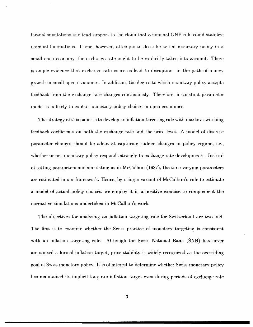
This paper extends McCallum’s (1987) nominal targeting rule to a small open economy by
allowing for feedback from the exchange rate. Instead of setting parameters in a McCallum-type
targeting rule and simulating, the parameters are estimated using a markov switching model. We
argue that a model of discrete parameter changes should be adept at capturing sudden changes in
policy regime, such as changes in the degree to which monetary policy admits feedback from the
exchange rate. We examine the legitimacy of an inflation targeting rule with occasional exchange-
rate feedback to describe Swiss monetary policy over the past twenty years.
KEYWORDS:. Inflation Targeting, Exchange Rate Feedback, Markov Switching
JEL CLASSIFICATION: C50, E52, E58
Michael DuekerEconomistFederal Reserve Bank of St. Louis411 Locust StreetSt. Louis, MO 63102
Andreas M. FischerSwiss National BankPostfach 8022Zurich, SWITZERLAND(41 1) 631 39 01Fax (41 1) 631 32 94

Inflation Targeting in a Small Open Economy:
Empirical Results for Switzerland
1. Introduction
The primary purpose ofnominal feedback rules for monetary policy ofthe type suggested
by McCallum (1987, 1988) is to prescribe a time path for an instrument variable which
would engender relatively smooth non-inflationary growth in nominal spending. Because
it appears unlikely, however, that a central bank would renounce discretion altogether and
adhere strictly to a rule, feedback rules have two likely empirical uses. The first is to
provide policymakers a reference to guide them in their instrument settings. Policymakers
could consult a nominal feedback rule, which is in line with their long-run inflation goal,
while retaining the flexibility to lessen short-term volatility in credit markets. The second
empirical use is to model past policy under the maintained hypothesis that monetary policy
has been implicitly following a feedback rule. By describing past policy with a feedback
rule, one can ascertain the implicit goals of past policy and when those goals appeared
to change. This article attempts to illustrate both empirical functions, using in-sample
results to describe Swiss monetary policy from 1974 to 1987 and out-of-sample results to
suggest how modeling monetary policy with a nominal feedback rule might provide useful
and timely information to policymakers.
Variants of McCallum’s GNP rule have been applied to the U.S. economy as well as
various small open economies.1 The empirical exercises concentrate primarily on counter-
‘See McCalIum (1993, 1994) for Japan and Hall (1990) for Germany, Japan, and Canada.
2
factual simulations and lend support to the claim that a nominal GNP rule could stabilize
nominal fluctuations. If one, however, attempts to describe actual monetary policy in a
small open economy, the exchange rate ought to be explicitly taken into account. There
is ample evidence that exchange rate concerns lead to disruptions in the path of money
growth in small open economies. In addition, the degree to which monetary policy accepts
feedback from the exchange rate changes continuously. Therefore, a constant parameter
model is unlikely to explain monetary policy choices in open economies.
The strategy of this paper is to develop an inflation targeting rule with markov-switching
feedback coefficients on both the exchange rate and the price level. A model of discrete
parameter changes should be adept at capturing sudden changes in policy regime, i.e.,
whether or not monetary policy responds strongly to exchange-rate developments. Instead
of setting parameters and simulating as in McCallum (1987), the time-varying parameters
are estimated in our framework. Hence, by using a variant of McCallum’s rule to estimate
a model of actual policy choices, we employ it in a positive exercise to complement the
normative simulations undertaken in McCallum’s work.
The objectives for analyzing an inflation targeting rule for Switzerland are two-fold.
The first is to examine whether the Swiss practice of monetary targeting is consistent
with an inflation targeting rule. Although the Swiss National Bank (SNB) has never
announced a formal inflation target, price stability is widely recognized as the overriding
goal of Swiss monetary policy. It is of interest to determine whether Swiss monetary policy
has maintained its implicit long-run inflation target even during periods of exchange rate
3

targeting and periods of above-normal inflation. The identification of a low implicit inflation
target represents a direct test of SNB claims that price stability is the primary objective
of Swiss monetary policy. The second objective is to carry the estimated model forward to
the 1988-94 period and examine its out-of-sample properties. The latter period followed a
major reduction in reserve requirements and the introduction of a new payments system,
and thus provides a test of McCallum’s criterion that a nominal targeting rule ought to be
impervious to financial innovations and regulatory changes.
The paper is organized as follows. Section 2 presents an informal account of Swiss
monetary policy since the end of the Bretton Woods system. A brief characterization of
this period is necessary in order to determine whether the empirical model generates results
consistent with known regime shifts. Section 3 presents the inflation targeting model with
markov switching. The model depicts an implicit inflation targeting rule which allows for
time-varying feedback from an exchange rate target. The estimation results for the 1974-
1987 period are presented in section 4. The same section also discusses the out-of-sample
performance of the model. Section 5 offers several conclusions.
2. General Features of Swiss Monetary Policy
“The Swiss National Bank has been setting monetary targets for well-nigh fifteen years.On several occasions however, notably in 1978, ii has had to deviate from its course forexchange rate reasons. If the principle of monetary targeting had been legally enforced,would we have violated the law or would we have allowed the Swiss franc to appreciatebeyond all reasonable limits? ... A central bank must thus be constantly on the alert andimplement its monetary target with the required flexibility.”
Markus Lusser, President of the Board of Governors, Swiss National Bank [Lusser
4

(1990) p. 183.]
The SNB has regularly announced monetary targets since the breakdown of the Bretton
Woods System.2 Rich (1995) reviews the SNB’s targetry framework and notes three policy
principles. First, price stability is recognized as the main and ultimate goal of monetary
policy. Second, the SNB’s position is that achievement of price stability is to be based on
the control of the money stock. Third, the targetry framework acts as a precommitment
device.
The SNB’s strategy ofannouncing monetary targets should not be interpreted as a strict
policy rule. Rather, the SNB’s approach to monetary targeting may best be described as
a contingent rule. The targets are designed to impose a medium to long-term constraint
on money growth with allowance for short-run flexibility to react to unanticipated shocks.
For instance, the SNB has made clear in its policy statements that it reserves the right to
intervene in the foreign exchange market when it feels that an excessive appreciation of the
Swiss franc could harm the real economy.
As in other countries, money growth targets are based on explicit inflation goals and
forecasts ofpotential output and velocity growth. Starting in 1975, the targets were first set
for the annual growth of the monetary aggregate Ml, where Ml was steered by a multiplier
model using the monetary base as the instrument. After a brief interlude of exchange-
rate targeting, annual monetary targets were set for the monetary base beginning in 1980.
2See Rich (1995) for a detailed account of Swiss monetary policy and Bernanke and Mishkin (1992) foran international comparison.
5
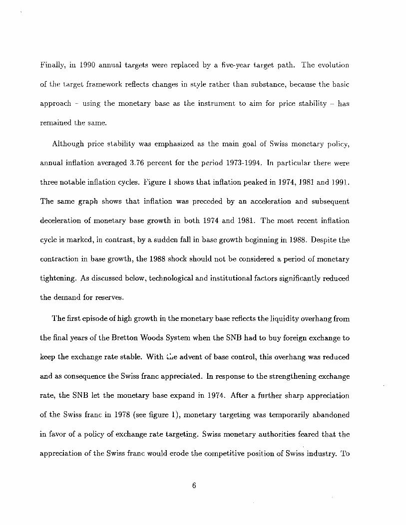
Finally, in 1990 annual targets were replaced by a five-year target path. The evolution
of the target framework reflects changes in style rather than substance, because the basic
approach using the monetary base as the instrument to aim for price stability — has
remained the same.
Although price stability was emphasized as the main goal of Swiss monetary policy,
annual inflation averaged 3.76 percent for the period 1973-1994. In particular there were
three notable inflation cycles. Figure 1 shows that inflation peaked in 1974, 1981 and 1991.
The same graph shows that inflation was preceded by an acceleration and subsequent
deceleration of monetary base growth in both 1974 and 1981. The most recent inflation
cycle is marked, in contrast, by a sudden fall in base growth beginning in 1988. Despite the
contraction in base growth, the 1988 shock should not be considered a period of monetary
tightening. As discussed below, technological and institutional factors significantly reduced
the demand for reserves.
The first episode ofhigh growth in the monetary base reflects the liquidity overhang from
the final years of the Bretton Woods System when the SNB had to buy foreign exchange to
keep the exchange rate stable. With ~ie advent of base control, this overhang was reduced
and as consequence the Swiss franc appreciated. In response to the strengthening exchange
rate, the SNB let the monetary base expand in 1974. After a further sharp appreciation
of the Swiss franc in 1978 (see figure 1), monetary targeting was temporarily abandoned
in favor of a policy of exchange rate targeting. Swiss monetary authorities feared that the
appreciation of the Swiss franc would erode the competitive position of Swiss industry. To
6

avert a potential slowdown in domestic activity, the SNB announced that it would keep
the exchange rate of the Deutsche mark above 0.80 Swiss francs. No monetary target
was announced for 1979. The foreign exchange rate interventions necessary to defend this
target resulted in an increase in the annual growth of the monetary base of over 25 percent.
The massive swings in the base growth during the 1978-1979 period, depicted in Figure 1,
capture the period of exchange rate targeting.
After returning to money supply targets in 1980, the SNB generally hit its base growth
targets through 1987. Actual base growth was below target in 1980 and 1981 when the
Swiss franc was weak. Then in 1982 and 1983, when the Swiss franc started to appreciate
again, endangering a still rather fragile economic recovery, actual base growth exceeded
the targets by small margins. A similar situation arose in 1987. In 1988 the demand for
base money underwent a permanent downward shift due to two factors: the introduction of
the Swiss Interbank Clearing (SIC) system and changes in reserve requirements.3 The SIC
accelerated the execution of payments and regulatory reforms brought both a reduction in
reserve requirements and a switch from contemporaneous to lagged reserve accounting. As
a result, the monetary base proved not to be a good indicator for monetary policy during
the transition period and the SNB had to look to other indicators such as broader monetary
aggregates, interest rates and the exchange rate.
At the risk of generalizing, the narrative approach identifies several periods when ex-
change rate considerations played a major role. The most significant is the 1978-1979
3See Vital and Mengle (1988) for a discussion regarding the SIC system.
7
period, when the monetary target was suspended and replaced by an explicit exchange rate
target. Less pronounced episodes include 1975 when the SNB resumed foreign exchange
interventions and the years between 1980 and 1983 when the SNB deviated slightly from
the monetary target in order to influence the exchange rate.
3. Description of the Empirical Model
Our indicator model with markov switching takes the monthly growth rate in the sea-
sonally adjusted monetary base less a forecasted growth rate for real base balances and
calls this “intended” inflation for the month. Assuming that the monetary base is the
instrument and that our forecasts mirror the general consensus at the time, our “intended”
inflation variable should reflect the policy intentions of the central bank across time. In the
model fluctuations in intended inflation come from three distinct sources: first, variation in
the central bank’s long-run inflation target; second, deviations from the price level target;
and, third, deviations from the exchange rate target.
The main equation of the feedback model is
Money growth:L~lnMB~= A0(Sl~)+ L~ln(~~)+ ~A1(Sl~){lni5— lnP]~_,P t~t-i
+~X2(S2~)[ln~— lne]~_1+ e(Sl~,S2~), (1)
E(Slt, SZ) student-f,
var[e(Slj,S2t)J = o2(S3~) —2’
where MB stands for the seasonally adjusted monetary base, P for the price level, and P
8

for the expected target level not conditional on the values of the state variables. Similarly,
e is the exchange rate and ~ is the expected target rate not conditional on the values of
the state variables. The error term E is assumed to have a student-f distribution with
n degrees of freedom. The forecast for real monetary base demand used to derive the
intended inflation rate is denoted by (MB/P)~1~_1.The Appendix discusses the derivation
of the forecasts for the real base growth. Three binary state variables Si, S2, and S3
are subject to markov switching:4 51 governs switching in parameters related to inflation
and/or price level targeting; S2 for parameters related to exchange-rate targeting; and S3
for heteroskedasticity.5 The notation a(S~)indicates that parameter a is subject to markov
switching governed by state variable S~.
The parameter ~ represents the long-run target rate of inflation, because intended
inflation will equal .A~when price-level and exchange-rate gaps equal zero in the long run.
Inferences of the state variable, Si, provide a probability-weighted estimate of the current
long-run inflation target: Prob.(Sl~= 0 Y~)x )t0(S1 = 0) + Prob.(Slt = 1 J Y~)x )~0(Sl=
1), where 1’ represents information available through time t. The sizes of the feedback
coefficients, )q(Slj) and .X2(S2j), determine the rate at which price~1eveland exchange-rate
gaps are gradually closed through policy actions.
The price level target and the exchange rate target are defined in equations (2) through
(5) to be a weighted average of last period’s actual and target levels. In the case of the
4The basic filtering and smoothing algorithms for a markov-switching model are discussed in Hamilton(1989).
5Kim (1993) notes that markov switching in the variance is an adept alternative to GARCH models formodeling conditional heteroskedasticity or “ARCH” effects.
9

price target, we also allow for trend growth, ~.
Target Price Level: lnP~(Sl~)= ~~(S1~) + ~,(Slt)ln~t_i + (1 — S1(Sl~))lnP~_1,(2)
Expected target: ln~ = ~ Prob(Sl~= i I Y~)ln~(S1~= i), (3)
Target Exch. Rate: lne~(S2~)= 62(S2~)ln~~_1+ (1 — 62(S2j))lne~_i, (4)
Expected target: ln~ = ~Prob(S2t = j I Y~)lne~(S2~= j). (5)
The variables P and ~ are, respectively, the target price level and the target exchange rate
conditional on particular values of the markov state variables. Rebasing of the target level
occurs for values of 5i, ~2 <1. Consequently, one-time shifts in the price level are gradually
accommodated into the target path. As S decreases from one, the degree to which the
target level is allowed to drift to accommodate recent developments increases. McCallum
(1993) has used an analogous weighting scheme; however, in his model ~1 remains constant.
Because of the autoregressive nature of equations (2) and (4), inferences of the state
at time t would depend on the entire history of past realizations of the state variables
if it were not for the collapsing procedure shown in equations (3) and (5). Kim (1994)
provides the justification for the collapsing procedure and notes that its use introduces
a small approximation to the evaluation of the likelihood function in a markov-switching
model. He finds, however, that the approximation does not materially affect the calculated
value of the likelihood function or the parameter estimates.
10

We define six transition probabilities for the three state variables:
P(Sl~= 0 I Sl~~= 0) = P1, (6)
P(S1~= 11 Sit_i = 1) = q1,
P(S2~= 0 I S2~_1= 0) = P2,
P(S2~= 11 S2~_1= 1) = q~,
P(S3t=0IS3~_i =0) =
P(S3~= 11 S3t—i = 1) = q3.
Implicit in equation (6) is an independence assumption that reduces the number of esti-
mated transition probabilities. In the general case with k state variables, each taking on
two values, one would need to estimate (2
k)2 — (2k) transition probabilities. Whereas with
the independence assumption, there are only 2k estimated parameters. In our model with
three state variables, the reduction due to the independence assumption is from 56 to 6
estimated parameters, making estimation feasible.
Maximum-likelihood estimates of the parameters are obtained by maximizing the log
of the expected likelihood or
in(~~ ~ Prob(Slt = i, S2~= j, S3~= k I Y~_1)LN’~) (7)
t=1 i=Oj=Ok=O
11

where the student-f densities are
= inF(.5(n + 1)) — lnF(.5n) — .51n(irnr2(S3t = k))
/ E(Sl~= i,S2~=j)~\—.5(n+l)ln~l+ ncr2(53t—k) ) (8)
and F is the gamma function.
4. Estimation Results and Interpretation
The monthly model is based on estimates for the 1974:1-1987:12 period. For the mon-
etary base (MB) a monthly average series is used, which takes account of the reserve
requirements effects.6 The consumer price index is used as the price variable (P), and the
Swiss franc/Deutsche mark exchange rate is used for (e). Both the series for MB and P
are seasonally adjusted. The data source is the SNB’s databank.
Three versions of the general model described by equations (1) to (6) are estimated
and summarized in Table 1. In Model 1 there is no feedback from the price level. Here
the estimated long-run inflation target (~X~)fluctuates within a relatively narrow band,
essentially between one and three percent. Without price-level feedback, the inflation rate
is targeted period-by-period. In the exchange-rate targeting, the degree of rebasing is
6Under the pre-1988 system of contemporaneous reserve accounting, the SNB enforced the reserverequirements at theend of each month. This created asharp rise in reserve demand and was accommodatedby the SNB to some extent. These end-of-month effects, also known as the ultimo effect, are averaged outin our series. In the out-of-sample period from 1988-1994, lagged reserve accounting prevailed. The reserverequirements are based on an average of the previous month. This resulted in the disappearance of theultimo effect. Therefore, a monthly seasonally adjusted figure for the monetary base was used for thepost-1988 period.
12

less than one in both states (62(82 = 0)=.832 and S2(82 = l)=.l37), implying, respetively,
gradual and relatively rapid accommodation of drift in the exchange rate target. Significant
conditional heteroskedasticity appears in the form of markov switching in the scale, a2(83)
of the variance. As in all heteroskedastic models, observations from the high-variance state
receive less weight. This implies that we are more cautious about inferring shifts in the
long-run inflation target, for example, when in the high-variance state.
Model 2 permits feedback from the price level, as opposed to period-by-period inflation
targeting, to affect base growth. Overall, the parameter estimates of Model 2 are similar to
those of Model 1. The feedback component for the price level is found to be insignificant
in both states. Tests of Model 1 against Model 2 are complicated by the fact that 6~is not
identified in Model 1. Thus, the likelihood-ratio test statistic does not have its standard
chi-square distribution. Nevertheless, the small difference of 0.97 between the log-likelihood
values of Models 1 and 2 and the insignificant feedback coefficients for prices ()~~)suggests
that Model l’s specification should not be rejected in favor of Model 2.
Model 3 restricts Model 1 to have a constant long-run inflation target, ~A0.In this
case two transition probabilities from Model 1, Pi and q1, are not identified under the null
of A0(Sl = 0) = .)~~(Sl= 1). Thus, the likelihood-ratio test statistic again has a non-
standard distribution, but the change in the log-likelihood from restricting )~is greater
than 25, which suggests that the restriction can be rejected.
Several graphs based on Model 1 are presented in order to illustrate the findings. In
all of the graphs, we have in-sample results through December 1987 and out-of-sample
13

results thereafter. Figure 2 plots a one-year moving average of actual Swiss inflation and
the model-implied inflation target, which varies between one and three percent. The low
level and narrow range of the model-implied inflation target lends credence to the SNB’s
claims that monetary targeting has been geared towards price stability.
Actual and model-implied quarterly growth of the Swiss monetary base are plotted in
figure 3. The model does not fit well the first few observations following the collapse of
the Bretton Woods system, before monetary targeting took hold. Between the mid-l970s
and 1987, however, the model-implied growth rates generally match the level and volatility
of base growth. In the post-1988 out-of-sample period, in particular, the model fulfills its
indicator function by pointing out that actual base growth between late 1989 and mid-
1992 was too strong to be consistent with inflation below three percent. Inflation began
to accelerate in late 1989, even though the official base target growth rate of one percent
was being slightly undershot due to a large shock to reserve demand which stemmed from
two sources: a change in reserve requirements and the introduction of the SIC system.
During this transition period, reserves fell from ten to three billion Swiss francs. Although
base growth contracted, it did not fall ‘~uick1yenough to accommodate the decrease in
the demand for base money. During this period, our indicator model suggests that base
growth should have been about two percentage per quarter lower to maintain inflation in
the one to three percent range (see figure 3). By mid-1992, the indicator model shows
that base growth was back on track to steer the inflation rate below three percent. Based
on the 1988-94 out-of-sample performance, we claim that the indicator model did not lose
14
relevance in the face of the sort of regulatory changes and technological financial innovations
that McCallurn (1988) contended a good nominal targeting procedure ought to sustain.
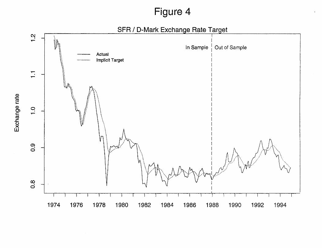
With respect to exchange-rate feedback, Figure 4 plots the model-implied exchange rate
target and the actual exchange rate. The graph shows that at times, notably in 1978 and
to a lesser extent in early 1982, the vertical distance between the two exchange rates is
relatively large. During these episodes the SNB raised base growth in an attempt to arrest
the appreciation of the Swiss franc.
Figure 5 takes the “exchange-rate gaps” from Figure 4 and multiplies them by the
feedback parameter, ~‘2, to estimate the influence exchange-rate feedback had on quarterly
money growth. This graph shows estimates of the portion of the 1978-79 surge in base
money growth that would be a response to the strong appreciation of the Swiss franc in
1978. The actual surge in base growth, however, was substantially larger than the model-
implied surge. Thus, base growth in 1978-79 might have been higher than necessary to
achieve the goal of stabilizing the value of the Swiss franc.
5. Conclusions
This paper develops an implicit inflation-targeting rule with exchange-rate feedback
and markov-switching parameters as an estimable model of Swiss monetary policy choices
regarding base money growth. The long-run inflation target is estimated to switch roughly
between one and three percent in the 1974-1987 period. The identification of such a narrow
band implies that, even when intervening on behalf of the exchange rate, the SNB was not
15

prepared to allow money growth to deviate for prolonged periods from the path implied
by either of two relatively low-inflation regimes. The post-1987 out-of-sample performance
reveals that the specification is robust to shocks stemming from changes in reserve require-
ments and technological innovations in the payments system, as such shocks greatly affected
the size and composition of the base starting in 1988. More importantly, our results show
that Swiss monetary policy would have been tighter during the most recent inflation cycle
if the implicit model had been used as a reference guide for SNB policymaking. The gap
between the actual and the model implied monetary base growth was closed gradually by
mid-1993 only after higher than normal inflation had been observed for more than three
years.
16
Appendix: Forecasts of Real Base Growth
The forecasts of real base growth for the in- and out-of-sample periods are based on a
model by Kim (1993). Let (MB/P) stand for the real monetary base, 3M0 the 3-month
Euro franc rate and P the consumer price index.7 The model generating the forecast is
Am = I?ot + flitA3MOt_i + /32~AinP~_,+ /33tAln (~~)+ ej,
Normal(0, he),
= o~+(o~—o-~)S~,S~E {0,l}, cr~>
Probabiiity(S~= 0 ~Sj_~ = 0) = P1,
Probability(S~= 1! ~ = 1) = P2~
The variances of the error terms are assumed to switch between a low and a high state
according to a first-order markov process. Persistence of low and high volatility states is
increasing in Pi and P2, respectively. The time-varying coefficients follow a random walk
process
= /3t~~1+Vt, v~’.’Normal(0,Q).
The random walk assumption implies that agents need information before changing their
views about the relationships among variables.
7Monthly measures of unemployment and real retail sales were found to be insignificant as explanatoryvariables.
17

References
Bernanke, B. and F. Mishkin, 1992, Central Bank Behavior and the Strategy of Mon-etary Policy, in 0. Blanchard and S. Fischer, eds., NBER Macroeconomics Annual, (MITPress, Cambridge) 183-228.
Hall, T. E., 1990, McCallum’s base growth rule: Results for the United States, WestGermany, Japan and Canada, Weltwirtschafthiches Archiv 126, 630-642.
Hamilton, J., 1989, A new approach to the economic analysis of nonstationary timeseries and the business cycle, Econometrica 57, 357-384.
Kim, C. J., 1993, Sources of money growth uncertainty and economic activity: The time-varying parameter with heteroskedastic disturbances, Review of Economics and Statistics,483-492.
Kim, C.J., 1994, Dynamic linear models with markov switching, Journal of Economet-rics 56, 1-22.
Lusser, M., 1990, Monetary policy and banking stability in: Zuhayr Mikdashi, ed.,Bankers’ and Public Authorities’ Management of Risks, (Macmillan, London).
McCallum, B. T., 1987, The case for rules in the conduct ofmonetary policy: A concreteexample, Economic Review, Federal Reserve Bank of Richmond, September/October, 10-18.
McCallum, B. T., 1988, Robustness properties of a rule for monetary policy, Carnegie-Rochester Conference Series on Public Policy 29, 173-204.
McCallum, B. T., 1993, Specification and analysis of a monetary policy rule for Japan,Bank of Japan Monetary and Economic Studies 11, 1-45.
McCallum, B. T., 1994, Monetary policy rules and financial stability, NBER WorkingPaper No. 4692.
Rich, G., 1995, Monetary targets as a policy rule: Lessons from Swiss experience, paperpresented at the Swiss National Bank conference on Rules versus Discretion in MonetaryPolicy, March 15-19, Gerzensee, Switzerland.
Vital, C. and D. L. Mengle, 1988, SIC: S~itzerland’s new electronic interbank paymentsystem, Federal Reserve Bank of Richmond, Economic Review, November/December, 12-27.
18

Table 1: Models of Inflation Targeting (eqns. 1-6): 1974:1-1987:12 Iparameter Model 1
no price feedbackModel 2
price feedbackModel 3constant inflation target
)~.~(Sl= 0)inflation target: low state
.844(.143)
.848(.137)
3.06(.127)
= 1)inflation target: high state
3.22(.114)
3.25(.119)
3.06(.127)
A1(Sl = 0)price level feedback
set to zero .758(.586)
set to zero
= 1)price_level_feedback
set to zero 0 set to zero
6,(Sl = 0)price_target_drift
set to zero 0 set to zero
t51(Sl = 1)price target drift
set to zero .772(.302)
set to zero
.A2(52 = 0)exchange rate feedback
.150(.058)
.132(.058)
.067(.084)
.X2(S2 = 1)exchange rate feedback
1.63(.227)
1.64(.226)
1.24(.288)
82(52 = 0)exch. rate target drift
.832(.105)
.861(.087)
.568(.021)
82(S2=l)exch. rate target drift
.137(.128)
.135(.128)
.825(.078)
cT2(53 = 0)low variance
.436(.082)
.437(.079)
.377(.114)
o~2(S3= 1)high variance
17.1(2.71)
16.7(2.67)
11.5(1.63)
Pi .903(.058)
.916(.050)
not estimated
q1 .971(.018)
.972(.017)
not estimated
P2 .999 .999 .988(.013)
q2.989
(.011).989
(.010).928(.047)
7~3 .972(.021)
.974(.020)
.909(.065)
q3 .976(.017)
.978(.017)
.980(.020)
Log-Likelihood -380.96 -379.99 -405.42No. of parameters 14 18 ii
Note: Standard errors are in parentheses
19

1
Figure 1Swiss Inflation, Base Money Growth, and Exchange Rate
0::
0
1.1
2()
0.9aLi-~ 0.8
1
~30 ~
U)
20 E~C’,10 ~C
-10 >-
I-C’,ci)>-
1975 77 79 81 83 85 87 89 91 93 95

Figure~2
Annual Inflation Rate
I I I I I I I I I I I I I I
Model implied target
co -
(0-
Inflation rate (One year MA) In Sample Out of SampleC)ctj0C)C)
C)
>0ECt,
C)C)C0
C)I0-
1975 1977 1979 1981 1983 1985 1987 1989 1991 1993 1995
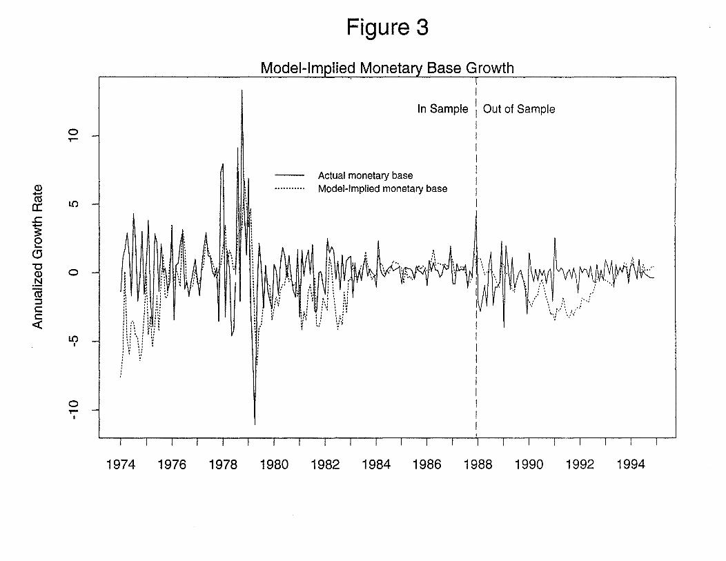
Figure 3
Model-Implied Monetary Base Growth
01~
LC) *
0-
Actual monetary baseC)Ct,
2C)N
Ct,
CC
In Sample Out of Sample
Model-Implied monetary base
0 -
I I I I I I I I I I I I I I I I I I I I I
1974 1976 1978 1980 1982 1984 1986 1988 1990 1992 1994
1~
1~
C).~
~) q-CCt,
C.)xw
C)0
Figure 4
SFR / D-Mark Exchanqe Rate Tarqet
I I I I 1 I I I I I~ if
1974 1976 1978 1980 1982 1984 1986 1988 1990 1992 1994
ActualImplicit Target
In Sample Out of Sample
0
I 1~ I I
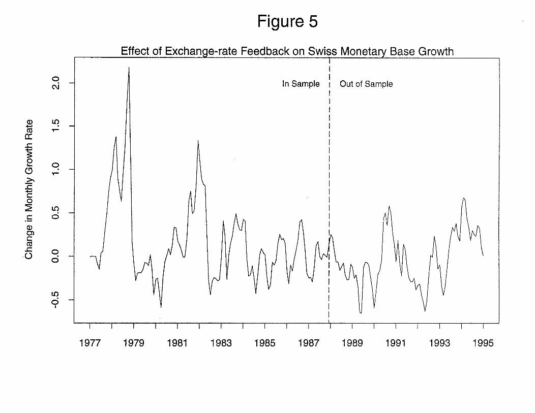
Figure 5
Effect of Exchange-rate Feedback on Sw~sMonetary Base Growth
I I I I I I II~~[ I
In Sample Out of Sample
C)
-C.~
2C!,>~
-CC0
C
C)C)CCt,
0
0C”
L
1~
Q
L
0
0d
U)
9
1977 1979 1981 1983 1985 1987 1989 1991 1993 1995
Top Related