


Languages
Pages
Legal


1
Inequality and Economic Growth
2014 MMSS Senior Thesis
Jihoon ko

2
Acknowledgements
I would like to thank Professor Joseph Ferrie, who, as a thesis advisor, has provided crucial
advices and support for writing my thesis. I also want to thank the MMSS program for providing
meaningful and rigorous academic training throughout my college years. I was fortunate enough to meet
friends and companions here who were always there to help me. I thank all of them. I thank Minji Kim,
who was there for me at the most crucial moments of my life and made it possible for me to become my
true self. I cannot stress enough how I love and thank my parents and my sister—I know that without
their full support and love, I couldn’t have come so far. Finally, thank God for giving me the true strength
to overcome the obstacles and develop through countless hardships.
3
Abstract
Significant amount of theories and analyses exist in the literature regarding the effect of
inequality on economic growth. The majority of them point to the conclusion that inequality is
detrimental to economic growth. This thesis performs two regressions, one for 1970-1980 and another for
1980-1990, to see if the relationship between inequality and the average annual growth rates changed. It
turns out that inequality had an effect on economic growth for 1980-1990, and a closer look into the Latin
American countries reveals that a crucial link is the economic policies. In the second part of this thesis,
series of analyses are performed to check if the inverted-U pattern predicted by the Kuznets curve had in
fact been a reality from 1970 to 1990. It becomes evident that the Kuznets curve does not show up clearly,
and that a cross-sectional analysis can be misleading.

4
Introduction
The word inequality has important political connotations. It is discussed frequently in media, and
it is not difficult to hear politicians uttering the word and pointing out that it is a serious problem.
However, when the term is mentioned, the focus is usually on social justice. Is there a practical reason to
worry about inequality? How does inequality affect growth? These questions became the central elements
of this thesis.
This thesis is consisted of two parts. The first part explores the impact of inequality on economic
growth. More specifically, it attempts to look at how a high level of income inequality affects economic
growth, and searches for possible links between the two. These analyses are meaningful in that it can help
people better understand inequality. If inequality turns out to be a negative factor in economic growth,
those who support the fight against inequality will have a stronger voice. In contrast, if inequality turns
out to be beneficial for economic growth, fighting inequality will mostly be a social justice issue, not an
economic or utilitarian one.
The second part looks at the relationship between an economy’s size and inequality. It is not
difficult to hear criticisms that recent economic growths have benefitted only a selected group of people
worldwide. Is it really the case? Is inequality a necessary byproduct of an economic progress, or does
economic growth decrease inequality because of its ‘trickle-down’ effect? This thesis provides analyses to
observe what happened as economies expanded from 1970 to 1990. They are meaningful because they
can help people get a more truthful picture of the impact of economic growth on inequality.
5
<Part I. Impact of Inequality on Economic Growth>
Literature Review
Several links between inequality and economic growth are discussed in the literature. The first
link is distributive policies implemented to fight inequality. Alesina and Rodrik (1994) apply the median
voter theorem to explain how this link operates. If income inequality is high, the median voter in the
economy will have an income lower than average income. Accordingly, majority of voters will prefer
redistributive policies, including progressive taxation, stronger minimum wage laws, and trade and capital
restrictions (Alesina and Rodrik 1994). Such economic policies will slow economic growth by their
distortionary effects, and even authoritarian regimes will not be able to completely ignore the majority’s
urge for redistribution for fear of being overthrown (Alesina and Rodrik 1994, Perotti 1995). More
specifically, redistributive policies and tax programs generate disincentives on private savings and
investment, both of which are crucial elements for economic growth (Perotti 1995). Therefore, an unequal
society might suffer a consequence of slowing down its economic growth by its distributive policies.
Another probable link is sociopolitical instability. Unequal distribution of income might create
incentives for individuals to engage in rent-seeking activities (Perotti 1995), and can cause riots, crimes,
or other disruptive activities (Barro 2000). These all lead to greater sociopolitical instability, which in turn
can be expected to decrease economic growth. Perotti (1995) points out that sociopolitical unrest reduces
investment because such instability creates political uncertainty, and directly reduces productivity as it
destroys market activities and labor relations. Therefore, an unequal economy might suffer economic
slowdown because it is more likely to be socio-politically unstable.
Barro (2000) argues that as credit markets are imperfect with asymmetric information and limited
capabilities of legal institutions, people’s abilities to take advantage of investment opportunities depend
on their levels of assets and incomes. In this case, redistribution of wealth from rich to poor raises the
total quantity and productivity of investment, given that such redistribution is distortion-free (Barro 2000).

6
Therefore, in an unequal society, many people will not be able to invest, and thus the overall economic
growth rates will become lower.
Inequality might have a negative impact on human capital accumulation. Perotti (1995) argues
that in an economy with high income inequality, more people are left unable to borrow against the future
income than those in a more equal economy. This might have a direct impact on human capital
investment, since fewer individuals will be able to afford education. Thus, a more equal society will have
higher growth rates, as more individuals will be able to invest in human capital. Galor and Zeira (1993)
present a similar result. Because of credit market imperfection, only those with sufficient income will be
able to afford education; moreover, because of indivisibility of human capital, the effects of this human
capital difference carry over to the long run. Therefore, according to Galor and Zeira (1993), only an
economy which have a large number of middle-class population will be able to achieve higher economic
growth rates in the long run.
Finally, Murphy, Shleifer, and Vishny (1989) demonstrate in their model that equality in income
distribution is important to secure a strong domestic market for economic growth. First, they argue that
leading industry sectors are needed for a country to initiate industrialization. However, in order for
industrialization to be sustainable, profits from a boom in the leading sector must be equally distributed
throughout the economy, because only by having equal distribution will an economy have a strong
domestic market for domestic manufactures (Murphy, Shleifer, and Vishny 1989). Although their model
only concerns closed economy or an economy with small open markets (Murphy, Shleifer, and Vishny
1989), it strongly indicates that equal distribution of income is crucial for a sustainable economic
development.
On the other hand, inequality might have positive effects on growth as well as negative ones.
Several studies point to this possibility. One argument is that higher inequality contributes to higher
overall level of investment in an economy. Kaldor (1957) provides an economic model in which a richer
7
group of people save but a poorer group of people cannot. According to this model, larger share of richer
people lead to large overall savings in the economy, and this results in a faster economic growth due to a
higher level of investment. Barro (2000) argues that if investment requires high setup costs, redistribution
of income might have negative effects on overall investment. For example, a business might be
unsuccessful at first but become productive after the investment reaches a threshold amount. In this case,
higher inequality indicates that the economy has a high number of wealthy people who are capable of
making such minimum investments, so higher inequality might actually be conducive to growth. In this
case, redistribution of income will lower the aggregate savings rate in an economy, thus slowing the
overall economic growth.
Saint-Paul and Verdier (1993) mention the effect of median voter’s interest in an unequal society
but in a different sense. They assert that in a democratic society, more economic inequality may promote
growth, because the median voter will likely support more powerful and effective public education, which
in turn works to improve human capital development and thus helps the economy grow. Therefore, in
contrast to Perotti (1995) and Galor and Zeira (1993), greater income inequality might actually lead to a
better education and faster economic growth.
Galor, Oded, and Tsiddon (1997) go further to argue that in an economy in an early stage of
development, inequality can even be necessary for future growth. They argue that because an individual’s
level of human capital is positively correlated to the parental level of human capital, economic inequality
helps the developing society to secure people with high levels of human capital, and the high levels of
human capital consequently help the economy grow. Therefore, an unequal society might actually
experience higher economic growth rates than more equal ones.
Given these extensive discussions about the possible impact of inequality on growth, the best way
to estimate the true relationship will be to perform regression analyses based on real-world data. Majority
of the empirical analyses, including Persson and Tabellini (1991), Alesina and Rodrik (1994), Perotti

8
(1996), and Deininger and Squire (1998), point to the conclusion that higher inequality is correlated with
lower economic growth. However, these analyses, except for Persson and Tabellini (1991), focus on a
single time period, rather than encompass multiple time periods. Choosing a single time period can lead to
an incomplete analysis, because there might be changes in the relationship between inequality and growth
across time periods. In order to detect any significant change in the relationship between inequality and
economic growth, two OLS regressions were performed separately for 1970-1980 and 1980-1990.
Detailed description about the regression equations and the data follows:
Regression Equations and Data
In an attempt to estimate the effect of inequality on economic growth, the following OLS
regression equations were used:
(1) Growth19701980i = B0 + B1IniGini70i + B2IniGDP70i + B3EduY70i + B4EduGapPY70i +
B5Investment70i + B6SPI7080i + r1LACi + ei
(2) Growth19801990i = B0 + B1IniGini80i + B2IniGDP80i + + B3EduY80i + B4EduGapPY80i +
B5Investment80i + B6SPI8090i + r1LACi + ei
Deininger and Squire (2006) suggest running regressions for sufficiently long periods because of
persistence of growth rates, and many other research on relationship between growth and inequality use at
least 10 years of data (Alesina and Rodrik 1994, Perotti 1995, Barro 2000). Following Deininger and
Squire’s advice, this thesis performed regressions over two 10-year periods, 1970 to 1980 and 1980 to
1990.
9
The dependent variable is 10-year average annual growth rate, calculated as compound annual
growth rate, from 1970 to 1980 in equation (1), and from 1980 to 1990 in equation (2). The most
important independent variable is Gini index, an indicator of income inequality, because our interest is
looking at the impact of inequality on economic growth. There may be many other factors that can affect
economic growth. However, it is impossible to write an exhaustive list of variables that should be
included, and this thesis choose not to include too many independent variables because doing so will
reduce the degrees of freedom substantially. Two variables, EduY and Investment, were included in each
regression equation to reflect the education levels and the relative size of overall investment in 1970 and
1980 within an economy. We also add sociopolitical instability, because it is plausible to assume that
sociopolitical instability will be detrimental to growth. These variables were included to avoid omitted
variable bias, as these are important factors in determining an economy’s growth rate. Also, these
variables reflect the factors that are commonly discussed, as shown in the literature review section, as
channels by which inequality may negatively affect growth. By including these variables, the equations (1)
and (2) will be able to capture the pure effect of inequality on economic growth, rather than the effect
complicated by these channels.
Gini coefficients, standard measures of income inequality, are in many cases of doubtful quality.
Countries often have different criteria in surveying their populations, base their figures on estimates rather
than on real data which are often uncollectible, and have different coverage, making any effort for cross-
national study about inequality subject to measurement errors and omitted variable bias (Forbes 2000). In
order to run cross-national regressions based on inequality, one needs a dataset that has been refined to
meet minimum standards.
Deininger and Squire (1996) compiled the available data on income inequality to create a
significantly improved dataset. They refined the data according to the following criteria: 1. Data should
be based on household surveys; 2. Data should have a comprehensive coverage of all significant sources
of income or uses of expenditure; 3. Data should represent national population. Based on these criteria,
10
Deininger and Squire gained 682 high-quality observations from 108 countries (Deinigner and Squire
1996). Their dataset contributed greatly to inequality research, as it could minimize measurement error
and any coefficient bias resulting from it, and thus increased the efficiency of estimates (Forbes 2000).
This thesis used the high-quality data as defined and gathered by Deininger and Squire (1996).
Even though their dataset is an excellent resource, it is not without complications. First, while this thesis
tries to measure the effect of inequality measures in 1970 on the following 10-year growth rates and 1980
measures on another 10-year growth rates, many countries in their dataset do not have Gini indices for
either 1970 or 1980. In such cases, inequality measures for the years closest to 1970 or 1980 were used.
Second, the data contains both Gini coefficients calculated from income data and those calculated from
expenditure data. Deininger and Squire (1996) points out that the Gini coefficients based on income is a
much better indicator of inequality—because coefficients calculated from expenditure data are based on
net incomes, inequality appears smaller because of progressive taxation. In order to remedy this problem,
they suggest adding 6.6 to the expenditure-based Gini coefficients, because the differences between
income-based Gini coefficients and expenditure-based Gini coefficients do not show a discernible pattern,
and the average difference between the two is 6.6 (Deininger and Squire 1996). However, while adding
6.6 to all the Gini coefficeints based on expenditure data can provide more data points, arbitrarily adding
6.6 to the different Gini coefficients can be oversimplifying. Therefore, this thesis only includes the Gini
coefficients based on income, even though doing so reduces the sample size substantially.
The data about initial per-capita GDP and economic growth rate are from World Development
Indicators, World Bank’s online resource. World Bank lists the time-series data of real per-capita GDPs
of 214 countries based on 2005 dollar. Initial per-capita GDPs were observed for the year corresponding
to the year from which the Gini coefficients were collected. The collected initial per-capita GDPs were
converted to natural logs. Then, annual growth rates for 1970-1980 and 1980-1990 were calculated for
each country as compound annual growth rates.

11
The data about education is based on Barro and Lee (2013). Barro (1997) points out that
secondary education tends to promote economic growth more than primary education does; this thesis
also uses the data about average years of secondary education for men and women for all the target
countries. However, special caution is needed when using the data about education. Barro and Lee (1994)
include both average years of secondary education for males and those for females in each country in
their growth regressions, and find out that the coefficient on female education is negative. They
hypothesize that the gender gap is indicative of economic backwardness, so the countries with better
female education levels have lower economic growth rates, because their economy is more developed
(Barro and Lee 1994). However, this hypothesis is rather counterintuitive, since higher female education
means a larger number of educated workers, who can provide important and competitive labor force. It
turns out that using both secondary education of men and that of women is problematic, because they are
very highly correlated. The correlation coefficient between the two in the database used for this thesis is
0.964 in 1970 and 0.967 in 1980. This almost perfect correlation questions the validity of the analysis that
include both male and female education levels because of multicollinearity issue.
One way to remedy the situation is to use a gender gap itself along with the total years of
education, because a country’s gender gap in education is not necessarily correlated with its level of
education. However, this approach is not without a problem, as gender gap in education in a country with
shorter average years of secondary education must be smaller than that with longer average years. Using
the gender gap in absolute terms can misrepresent a country with shorter average years of education to be
fair in education across genders, and this runs a risk of ignoring completely the relative gender inequality,
which is of interest in this thesis.
In order to deal with this complication, this thesis introduces new variables, EduGapPY70 and
EduGapPY80, which are derived by dividing a country’s gender difference in average years of secondary
education by its average years of secondary education for the entire population. This approach
successfully avoids a possible bias because of differences in average years of secondary education, as it is
12
measuring gender inequality in education in a relative term, not in an absolute term. Also, while it is true
that EduGapPY70 and EduGapPY80 are still somewhat correlated with EduY70 and EduY80, introducing
these variables successfully avoid the problem of almost perfect collinearity posed by including separate
variables for male education and female education.
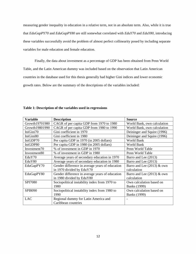
Finally, the data about investment as a percentage of GDP has been obtained from Penn World
Table, and the Latin American dummy was included based on the observation that Latin American
countries in the database used for this thesis generally had higher Gini indices and lower economic
growth rates. Below are the summary of the descriptions of the variables included:
Table 1: Description of the variables used in regressions
Variable Description Source
Growth19701980 CAGR of per capita GDP from 1970 to 1980 World Bank, own calculation
Growth19801990 CAGR of per capita GDP from 1980 to 1990 World Bank, own calculation
IniGini70 Gini coefficient in 1970 Deininger and Squire (1996)
IniGini80 Gini coefficient in 1980 Deininger and Squire (1996)
IniGDP70 Per capita GDP in 1970 (in 2005 dollars) World Bank
IniGDP80 Per capita GDP in 1980 (in 2005 dollars) World Bank
Investment70 % of investment in GDP in 1970 Penn World Table
Investment80 % of investment in GDP in 1980 Penn World Table
EduY70 Average years of secondary education in 1970 Barro and Lee (2013)
EduY80 Average years of secondary education in 1980 Barro and Lee (2013)
EduGapPY70 Gender difference in average years of education
in 1970 divided by EduY70
Barro and Lee (2013) & own
calculation
EduGapPY80 Gender difference in average years of education
in 1980 divided by EduY80
Barro and Lee (2013) & own
calculation
SPI7080 Sociopolitical instability index from 1970 to
1980
Own calculation based on
Banks (1999)
SPI8090 Sociopolitical instability index from 1980 to
1990
Own calculation based on
Banks (1999)
LAC Regional dummy for Latin America and
Caribbean countries
-

13
Construction of Sociopolitical Instability Index
It is very difficult to measure social instability. The actual degree of sociopolitical instability
perceived by the public is naturally an extremely difficult, if not impossible, concept to quantify. Given
this unclear nature of sociopolitical instability, the second best way to represent the degree of
sociopolitical instability is to construct an estimate of it based on actual counts of the events that can
cause a country to become socio-politically more unstable. In an attempt to do this, sociopolitical
instability indices for the countries in question were constructed by following the steps below.
1. Selection of Data and Variables
The Cross-National Time-Series Database from Banks (1999) provides a vast resource from
which to construct the sociopolitical indices. It includes actual counts of major social and political events
from 1970 to 1990, the target time period of this study. Among the events included in the database, this
thesis selected the ones that are most likely to result in significant sociopolitical instability: assassinations,
strikes, guerrilla warfare, government crises, purges, riots, revolutions, anti-government demonstrations,
and coup de tats.
2. Calculation of Sociopolitical Instability Index
Although it is a comprehensive database, the Banks database has a number of problems. First, the
variables are the actual counts of occurrences; therefore, populous countries naturally tend to have higher
values. Considering the mere counts of events will certainly lead to a faulty conclusion that countries with
more people are socio-politically more unstable. Second, the variables change significantly from year to
year for a given country. This is natural, since the same country may have a high degree of sociopolitical
instability in a certain year and then stabilize in the following year, and vice versa. Thus, it is a serious
14
mistake to look only at the variables from a certain year and draw conclusions about sociopolitical
instability of that country.
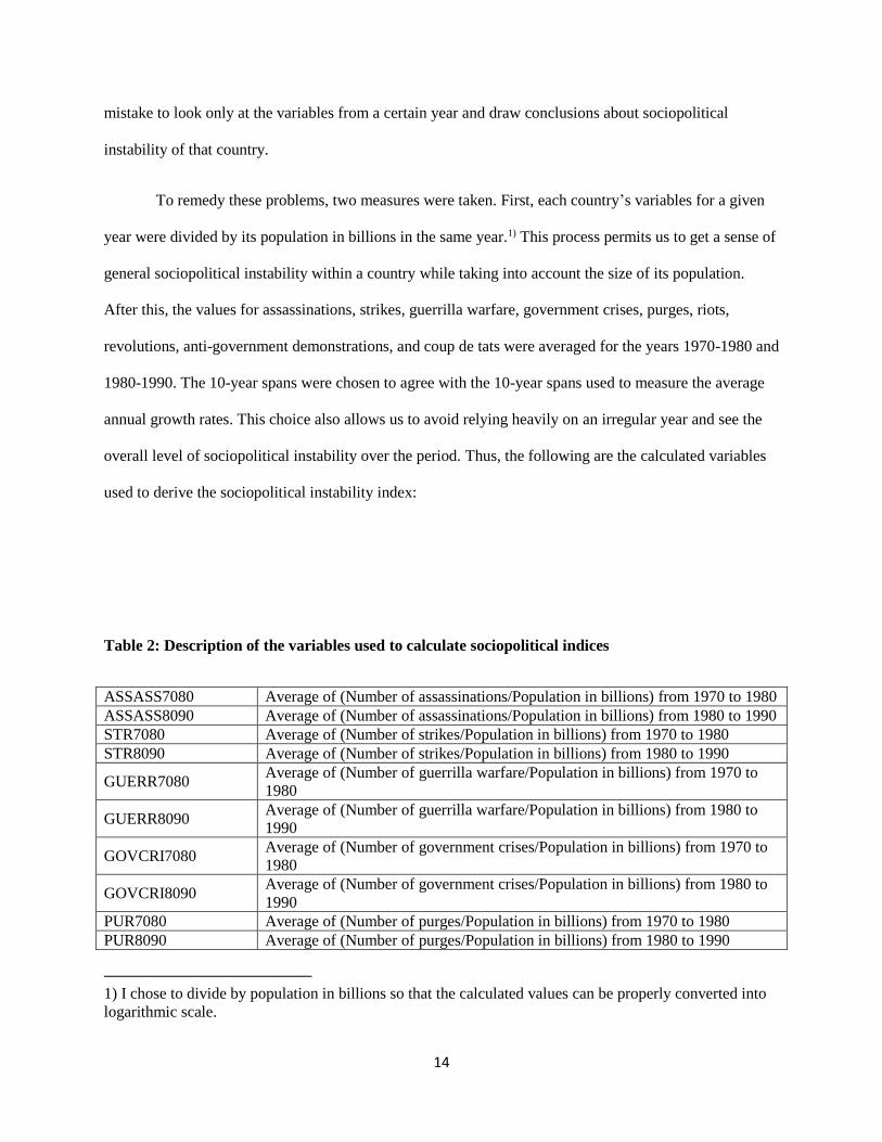
To remedy these problems, two measures were taken. First, each country’s variables for a given
year were divided by its population in billions in the same year.1) This process permits us to get a sense of
general sociopolitical instability within a country while taking into account the size of its population.
After this, the values for assassinations, strikes, guerrilla warfare, government crises, purges, riots,
revolutions, anti-government demonstrations, and coup de tats were averaged for the years 1970-1980 and
1980-1990. The 10-year spans were chosen to agree with the 10-year spans used to measure the average
annual growth rates. This choice also allows us to avoid relying heavily on an irregular year and see the
overall level of sociopolitical instability over the period. Thus, the following are the calculated variables
used to derive the sociopolitical instability index:
Table 2: Description of the variables used to calculate sociopolitical indices
ASSASS7080 Average of (Number of assassinations/Population in billions) from 1970 to 1980
ASSASS8090 Average of (Number of assassinations/Population in billions) from 1980 to 1990
STR7080 Average of (Number of strikes/Population in billions) from 1970 to 1980
STR8090 Average of (Number of strikes/Population in billions) from 1980 to 1990
GUERR7080 Average of (Number of guerrilla warfare/Population in billions) from 1970 to
1980
GUERR8090 Average of (Number of guerrilla warfare/Population in billions) from 1980 to
1990
GOVCRI7080 Average of (Number of government crises/Population in billions) from 1970 to
1980
GOVCRI8090 Average of (Number of government crises/Population in billions) from 1980 to
1990
PUR7080 Average of (Number of purges/Population in billions) from 1970 to 1980
PUR8090 Average of (Number of purges/Population in billions) from 1980 to 1990
1) I chose to divide by population in billions so that the calculated values can be properly converted into
logarithmic scale.
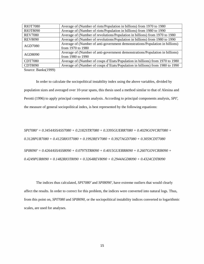
15
RIOT7080 Average of (Number of riots/Population in billions) from 1970 to 1980
RIOT8090 Average of (Number of riots/Population in billions) from 1980 to 1990
REV7080 Average of (Number of revolutions/Population in billions) from 1970 to 1980
REV8090 Average of (Number of revolutions/Population in billions) from 1980 to 1990
AGD7080 Average of (Number of anti-government demonstrations/Population in billions)
from 1970 to 1980
AGD8090 Average of (Number of anti-government demonstrations/Population in billions)
from 1980 to 1990
CDT7080 Average of (Number of coups d’Etats/Population in billions) from 1970 to 1980
CDT8090 Average of (Number of coups d’Etats/Population in billions) from 1980 to 1990
Source: Banks(1999)
In order to calculate the sociopolitical instability index using the above variables, divided by
population sizes and averaged over 10-year spans, this thesis used a method similar to that of Alesina and
Perotti (1996) to apply principal components analysis. According to principal components analysis, SPI′,
the measure of general sociopolitical index, is best represented by the following equations:
SPI7080′ = 0.3454ASSASS7080 + 0.2182STR7080 + 0.3395GUERR7080 + 0.4029GOVCRI7080 +
0.3128PUR7080 + 0.4125RIOT7080 + 0.1992REV7080 + 0.3927AGD7080 + 0.3059CDT7080
SPI8090′ = 0.4264ASSASS8090 + 0.0797STR8090 + 0.4015GUERR8090 + 0.2607GOVCRI8090 +
0.4249PUR8090 + 0.1482RIOT8090 + 0.3264REV8090 + 0.2944AGD8090 + 0.4324CDT8090
The indices thus calculated, SPI7080′ and SPI8090′, have extreme outliers that would clearly
affect the results. In order to correct for this problem, the indices were converted into natural logs. Thus,
from this point on, SPI7080 and SPI8090, or the sociopolitical instability indices converted to logarithmic
scales, are used for analyses.

16
Results & Interpretations
Below is the summary of the results of the OLS regressions:
Table 3: Results of the Regressions
Growth rate 1970~1980 1970~1980 1980~1990 1980~1990
IniGDP 70 / 80 -0.0064
(0.0039)
-0.0074
(0.0040)
-0.0071
(0.0046)
-0.0074
(0.0046)
IniGini 70 / 80 -0.0438
(0.0383)
-0.0055
(0.0477)
-0.1013
(0.0445)
-0.0703
(0.0535)
EduY 70/80 -0.0006
(0.0037)
-0.0019
(0.0037)
0.0083
(0.0040)
0.0068
(0.0042)
EduGapPY 70 / 80 0.0066
(0.0125)
-0.0109
(0.0183)
0.0096
(0.0177)
-0.0004
(0.0201)
Investment 70 / 80 0.0696
(0.0278)
0.0774
(0.0280)
0.0891
(0.0366)
0.0529
(0.0504)
SPI7080/8090 -0.0035
(0.0034)
-0.0032
(0.0034)
-0.0057
(0.0038)
-0.0060
(0.0038)
LAC - -0.0152
(0.0116)
- -0.0126
(0.0121)
Constant 0.0983
(0.0436)
0.0991
(0.0429)
0.0972
(0.0571)
0.1063
(0.0576)
# of observations 30 30 40 40
R2 0.31 0.36 0.42 0.44
(Numbers in parentheses indicate standard errors.)
Some interesting observations can be made. For the regression equations with the average annual
growth rates from 1970 to 1980 as the dependent variable, all the coefficients except the one on
investment are insignificant. Investment is the only statistically significant factor—the coefficient on it is
positive with 0.0696 and has a t-statistic of 2.50 when the Latin American dummy variable is excluded,
and it increases even more to 0.0774 with t-statistic of 2.76 when the Latin American dummy is included.
Therefore, we can reject the null hypothesis at 95% level and 99% level, respectively. The coefficient on
GDP with the inclusion of Latin American dummy is -0.0074 with t-statistic of -1.87, so we can reject the
null hypothesis at 90% level. Sociopolitical instability seems to have had negative effect on growth, but
17
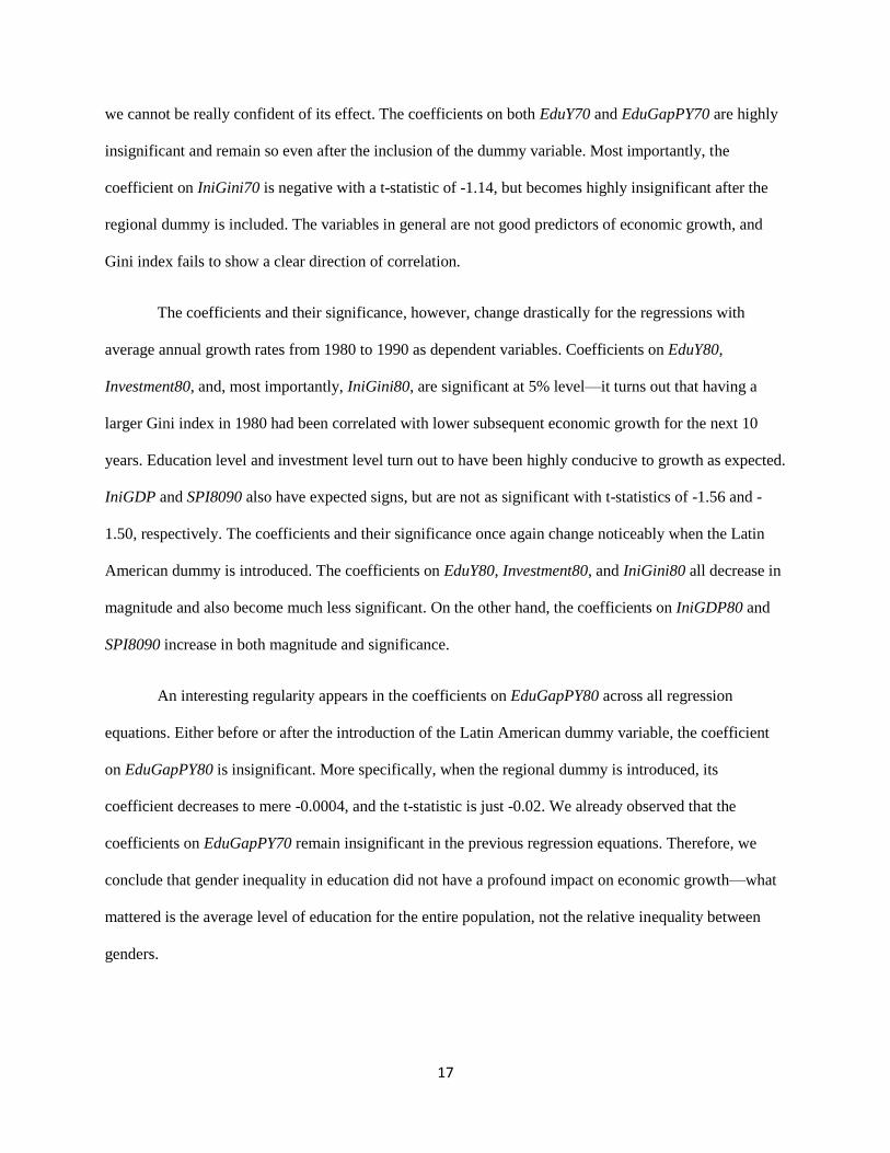
we cannot be really confident of its effect. The coefficients on both EduY70 and EduGapPY70 are highly
insignificant and remain so even after the inclusion of the dummy variable. Most importantly, the
coefficient on IniGini70 is negative with a t-statistic of -1.14, but becomes highly insignificant after the
regional dummy is included. The variables in general are not good predictors of economic growth, and
Gini index fails to show a clear direction of correlation.
The coefficients and their significance, however, change drastically for the regressions with
average annual growth rates from 1980 to 1990 as dependent variables. Coefficients on EduY80,
Investment80, and, most importantly, IniGini80, are significant at 5% level—it turns out that having a
larger Gini index in 1980 had been correlated with lower subsequent economic growth for the next 10
years. Education level and investment level turn out to have been highly conducive to growth as expected.
IniGDP and SPI8090 also have expected signs, but are not as significant with t-statistics of -1.56 and -
1.50, respectively. The coefficients and their significance once again change noticeably when the Latin
American dummy is introduced. The coefficients on EduY80, Investment80, and IniGini80 all decrease in
magnitude and also become much less significant. On the other hand, the coefficients on IniGDP80 and
SPI8090 increase in both magnitude and significance.
An interesting regularity appears in the coefficients on EduGapPY80 across all regression
equations. Either before or after the introduction of the Latin American dummy variable, the coefficient
on EduGapPY80 is insignificant. More specifically, when the regional dummy is introduced, its
coefficient decreases to mere -0.0004, and the t-statistic is just -0.02. We already observed that the
coefficients on EduGapPY70 remain insignificant in the previous regression equations. Therefore, we
conclude that gender inequality in education did not have a profound impact on economic growth—what
mattered is the average level of education for the entire population, not the relative inequality between
genders.
18
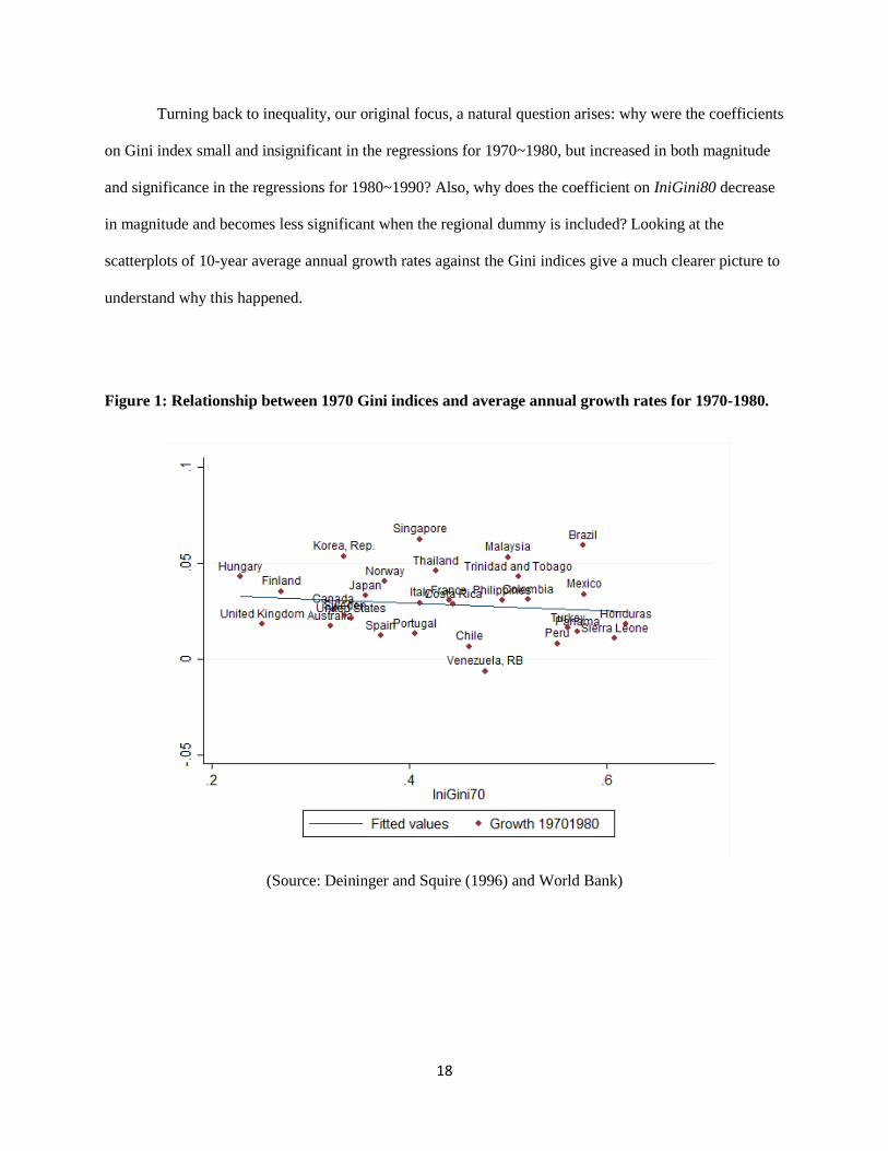
Turning back to inequality, our original focus, a natural question arises: why were the coefficients
on Gini index small and insignificant in the regressions for 1970~1980, but increased in both magnitude
and significance in the regressions for 1980~1990? Also, why does the coefficient on IniGini80 decrease
in magnitude and becomes less significant when the regional dummy is included? Looking at the
scatterplots of 10-year average annual growth rates against the Gini indices give a much clearer picture to
understand why this happened.
Figure 1: Relationship between 1970 Gini indices and average annual growth rates for 1970-1980.
(Source: Deininger and Squire (1996) and World Bank)

19
Figure 2: Relationship between 1980 Gini indices and average annual growth rates for 1980-1990.
(Source: Deininger and Squire (1996) and World Bank)
Average annual growth rates from 1970 to 1980 were plotted against Gini indices in 1970, and
those from 1980 to 1990 were plotted against Gini indices in 1980. As shown in Figure 1, for 1970~1980
there is no significant correlation between Gini coefficients and subsequent growth rates. However, for
1980~1990, a clear negative correlation appears, as shown evidently in Figure 2. Asian countries are at
the upper left corner, and those located at the bottom right corner, with high inequality and negative
economic growths, are predominantly Latin American countries. This explains why the coefficient on
Gini index changed for 1980-1990 and then changes again substantially after including the Latin
American dummy. Looking at the individual countries on the bottom right corner will provide a valuable
insight to understand the relationship between inequality and economic growth, and the deeper look into
the situations in the Latin American countries is the focus of the next chapter.
20
Case for Latin America—Potential Dangers of ‘Populist’ Policies
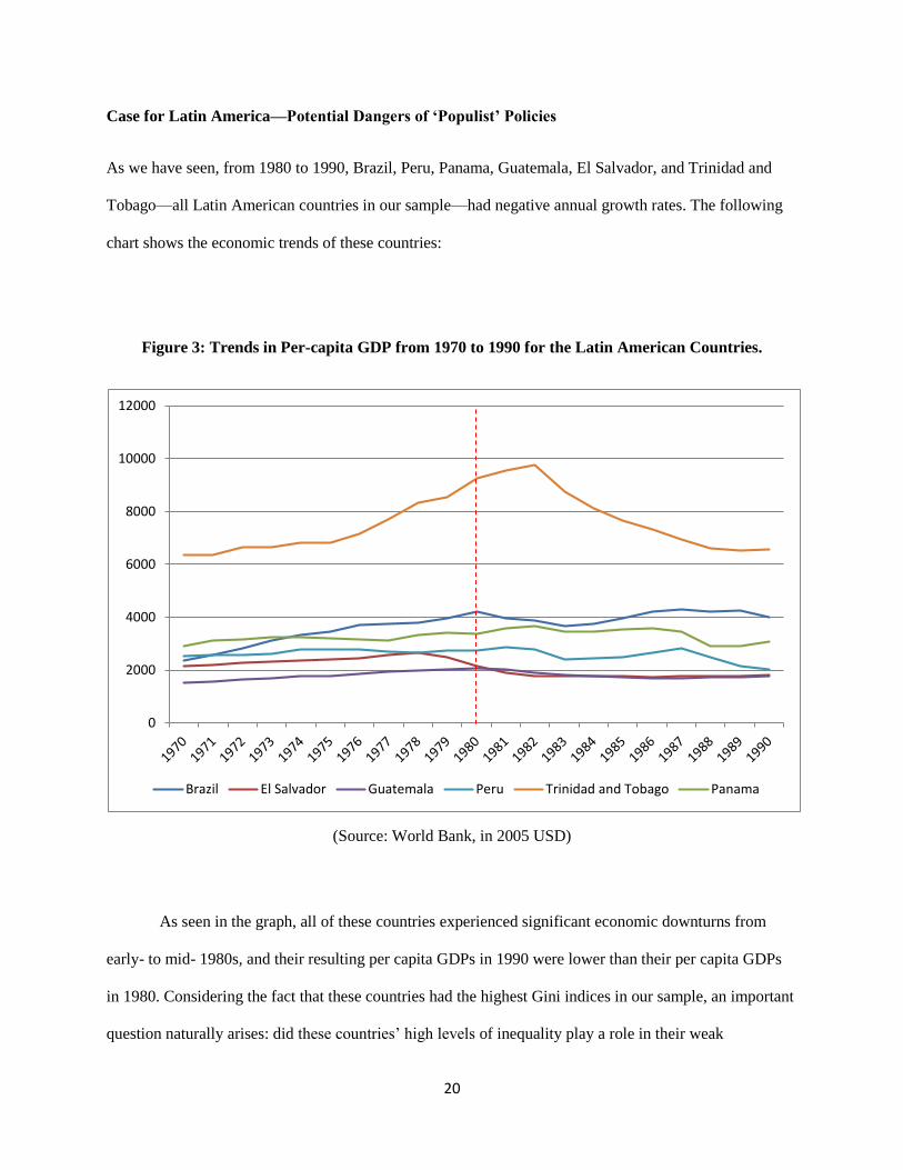
As we have seen, from 1980 to 1990, Brazil, Peru, Panama, Guatemala, El Salvador, and Trinidad and
Tobago—all Latin American countries in our sample—had negative annual growth rates. The following
chart shows the economic trends of these countries:
Figure 3: Trends in Per-capita GDP from 1970 to 1990 for the Latin American Countries.
(Source: World Bank, in 2005 USD)
As seen in the graph, all of these countries experienced significant economic downturns from
early- to mid- 1980s, and their resulting per capita GDPs in 1990 were lower than their per capita GDPs
in 1980. Considering the fact that these countries had the highest Gini indices in our sample, an important
question naturally arises: did these countries’ high levels of inequality play a role in their weak
0
2000
4000
6000
8000
10000
12000
Brazil El Salvador Guatemala Peru Trinidad and Tobago Panama
21
performances, or did another factor negatively affect their economies? When viewed carefully, it becomes
evident that inequality played a role in the deterioration of their economies, and the primary channel turns
out to be unsuccessful economic policies that aimed at reducing inequality.
Sachs (1989) explains the case for Brazil. In 1985, Jose Sarney became the president of Brazil.
His government implemented strong populist measures to assuage the public’s discontent over inequality,
which have increased substantially after four years of austerity measures following the debt crisis in the
beginning of the decade. In implementing the so-called Cruzado plan, the government increased the real
wages, overvalued the domestic currency, and ran a budget deficit (Sachs 1989). These measures,
combined with the large amount of inherited debt, quickly backfired. Trade deficit worsened, and the
government had to devalue its currency in order to avoid a reserve crisis. As a result, inflation
skyrocketed and the economic growth rate of Brazil again turned negative. The policies to fight inequality,
which were successful at first, worked to make the Brazilian economy even worse.
Sachs (1989) mentions Peru as another example of a country whose faulty economic policies
made the situation much worse. After Alan Garcia became a president in 1985, he implemented a series
of powerful economic policies, including suspension of debt-servicing payments, increase in public sector
prices, freeze on exchange rate, and a substantial raise in public sector wages (Sachs 1989). These
measures were executed with the intention to fight inequality and reverse the weak performance of the
Peruvian economy. His policies were highly successful at first, but eventually led to a deficit in trade
balance, appreciation of real exchange rates, and depletion of foreign exchange reserves in 1988.
Hyperinflation and a rapid collapse of the economy followed. As seen in figure 3, Peru’s real per-capita
GDP, which increased significantly from 1985 to 1987, experienced a steep decrease from 1987 to
1990—the unsuccessful economic policies certainly contributed to this collapse.
Looking at the cases of Brazil and Peru in 1980s, the political link between inequality and
worsening of the economy becomes clear. Granted, these countries had suffered greatly because of the
22
severe Latin American debt crisis in the early 1980s, and it definitely was a decisive factor in worsening
their economies (Sachs 1989). Nevertheless, the unsuccessful policies aimed at fighting inequality made
situations even worse. The policies implemented by these two countries are not necessarily unique to
Latin America. Politicians in any country with a high degree of inequality might implement powerful
redistributive policies any time, either because a median voter will favor such policy or because they
might be tempted to do so in order to gain widespread support. As seen in the examples of Brazil and
Peru, such policies can eventually backfire. Therefore, countries with higher income inequality are more
likely to experience economic problems stemming from unsuccessful policy measures. This is confirmed
by Berg and Sachs (1988), in which the authors find that the countries with higher inequalities were far
more likely to experience debt rescheduling.
23
<Part II. Relationship between economy’s size and inequality>
Literature Review
Simon Kuznets (1955) asserted that an economy’s inequality initially increases following a period
of economic growth, and then decreases after the economy reaches a certain level. Therefore, when the
measure of inequality is plotted against the size of the economy, it will follow an inverted-U pattern
(Kuznets 1955). This hypothesis, popularly known as the Kuznets curve, is based on the premise that an
economy is initially largely based on agriculture. As the economy advances and is urbanized, people
begin to migrate into cities, where incomes are much higher, thereby increasing the overall income
inequality between urban, industrial sectors and rural, agricultural sectors within the economy (Kuznets
1955). However, after the economy reaches a certain level, the fruits of industrialization begin to spread
to the economy, and overall level of inequality would eventually decrease (Kuznets 1955). The natural
question to ask is: had it been the case for 1970-1990, the time period covered in part I?
This part of the thesis aims to check if Kuznets curve actually appeared during the 20-year time
period to explore the relationship between economic growth and inequality. The results, even though they
are based on past data, will also be useful for modern days in that they will assist in an effort to better
understand the underlying relationship between economic growth and inequality—more specifically,
whether there is actually a trickle-down effect or winners take all as economy develops.
Analysis
First, using the same data as those used in part I, the countries’ Gini indices in 1970 were plotted
against the log of per-capita GDPs in 1970. Then, the Gini indices in 1980 were plotted against the log of
per-capita GDPs in 1980. The results are shown below:
24
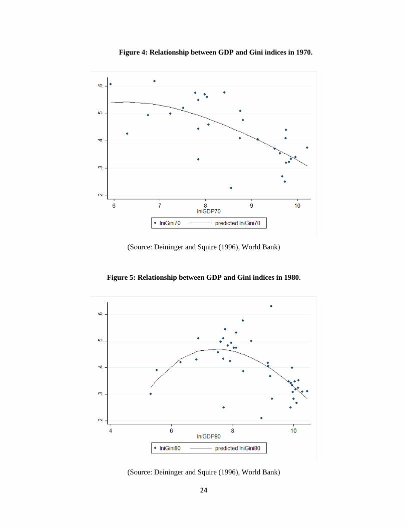
Figure 4: Relationship between GDP and Gini indices in 1970.
(Source: Deininger and Squire (1996), World Bank)
Figure 5: Relationship between GDP and Gini indices in 1980.
(Source: Deininger and Squire (1996), World Bank)

25
As seen in figure 4, in 1970, a negative correlation between per-capita GDP and Gini indices
appears, but an inverted-U pattern predicted by Kuznets curve is not obvious. On the other hand, in 1980,
a clear inverted-U pattern appears. Regression analysis was performed to confirm the apparent existence
of Kuznets curve. Below are the results from the set of OLS regressions to estimate the relationship
between the sizes of the economy and per-capita GDPs:
Table 4: Results of cross-national regressions to test the existence of Kuznets curve
IniGini70 IniGini80
IniGDP70/IniGDP80 0.135
(0.182)
0.368
(0.102)
(IniGDP70)2 /
(IniGDP80)2
-0.012
(0.011)
-0.024
(0.006)
Constant 0.164
(0.745)
-0.934
(0.413)
R2 0.47 0.41
#. of observations 30 40
(Numbers in parenthesis refer to standard errors.)
The regression equations had Gini coefficients in 1970 and 1980 as dependent variables, and real
per-capita GDP in 1970 and 1980 and a quadratic term of real per-capita GDP in 1970 and 1980 as
independent variables. As can be easily observed, the coefficient on per-Capita GDP in the 1980
regression equation is positive with a t-statistic of almost 3.6, and the coefficient on the quadratic term in
the same regression equation is negative and highly significant with the t-statistic nearing almost -4.
Therefore, while no definite pattern is detected for 1970, the cross-national analysis seems to confirm the
actual existence of Kuznets curve in 1980.
Nevertheless, it can be misleading to draw conclusions about the existence of Kuznets curve from
a cross-national analysis. It is very tempting to conclude that Kuznets curve appears to have been a clear
empirical regularity in 1980 based on the results above. However, it is important to keep in mind that
Kuznets curve is a theory about changes in inequality within a country as its economy becomes larger
26
(Kuznets 1955). Therefore, deciding from the results of the cross-country analyses that inequality
followed an inverted-U pattern can be misleading. Because the countries had different levels of inequality,
different degrees of changes in the size of the economy, and distinct characteristics unique to themselves
that might make the cross-national analyses invalid, a better analysis to test the Kuznets curve is
observing the patterns of inequality against time within each country.
Therefore, this thesis implemented a different analysis, measuring the relationship between
income inequality and GDP of each country. Available data of GDPs and Gini indices were collected
from 1970 to 1990 for each country. Then, in order to avoid a potential problem from having too little
number of observations, only the countries with at least 5 observations of Gini indices over the time
period were included. For the 27 countries that survived the screening, dummy variables were assigned to
make the derivation of coefficients unique to each country possible. Then, the available Gini indices were
regressed against the available per-capita GDPs and its squared term for each country. The results of this
OLS regression are summarized in the following table:
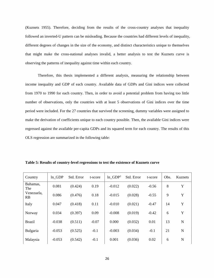
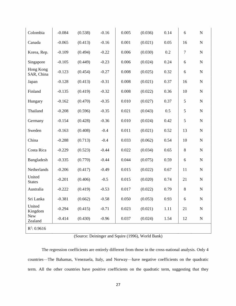
Table 5: Results of country-level regressions to test the existence of Kuznets curve
Country ln_GDP Std. Error t-score ln_GDP2 Std. Error t-score Obs. Kuznets
Bahamas,
The 0.081 (0.424) 0.19 -0.012 (0.022) -0.56 8 Y
Venezuela,
RB 0.086 (0.476) 0.18 -0.015 (0.028) -0.55 9 Y
Italy 0.047 (0.418) 0.11 -0.010 (0.021) -0.47 14 Y
Norway 0.034 (0.397) 0.09 -0.008 (0.019) -0.42 6 Y
Brazil -0.038 (0.511) -0.07 0.000 (0.032) 0.01 13 N
Bulgaria -0.053 (0.525) -0.1 -0.003 (0.034) -0.1 21 N
Malaysia -0.053 (0.542) -0.1 0.001 (0.036) 0.02 6 N
27
Colombia -0.084 (0.538) -0.16 0.005 (0.036) 0.14 6 N
Canada -0.065 (0.413) -0.16 0.001 (0.021) 0.05 16 N
Korea, Rep. -0.109 (0.494) -0.22 0.006 (0.030) 0.2 7 N
Singapore -0.105 (0.449) -0.23 0.006 (0.024) 0.24 6 N
Hong Kong
SAR, China -0.123 (0.454) -0.27 0.008 (0.025) 0.32 6 N
Japan -0.128 (0.413) -0.31 0.008 (0.021) 0.37 16 N
Finland -0.135 (0.419) -0.32 0.008 (0.022) 0.36 10 N
Hungary -0.162 (0.470) -0.35 0.010 (0.027) 0.37 5 N
Thailand -0.208 (0.596) -0.35 0.021 (0.043) 0.5 5 N
Germany -0.154 (0.428) -0.36 0.010 (0.024) 0.42 5 N
Sweden -0.163 (0.408) -0.4 0.011 (0.021) 0.52 13 N
China -0.288 (0.713) -0.4 0.033 (0.062) 0.54 10 N
Costa Rica -0.229 (0.523) -0.44 0.022 (0.034) 0.65 8 N
Bangladesh -0.335 (0.770) -0.44 0.044 (0.075) 0.59 6 N
Netherlands -0.206 (0.417) -0.49 0.015 (0.022) 0.67 11 N
United
States -0.201 (0.406) -0.5 0.015 (0.020) 0.74 21 N
Australia -0.222 (0.419) -0.53 0.017 (0.022) 0.79 8 N
Sri Lanka -0.381 (0.662) -0.58 0.050 (0.053) 0.93 6 N
United
Kingdom -0.294 (0.415) -0.71 0.023 (0.021) 1.11 21 N
New
Zealand -0.414 (0.430) -0.96 0.037 (0.024) 1.54 12 N
R2: 0.9616
(Source: Deininger and Squire (1996), World Bank)
The regression coefficients are entirely different from those in the cross-national analysis. Only 4
countries—The Bahamas, Venezuela, Italy, and Norway—have negative coefficients on the quadratic
term. All the other countries have positive coefficients on the quadratic term, suggesting that they

28
experienced increases in inequality as their economies grew. While the coefficients are mostly
insignificant, the clear evidence of Kuznets curve derived in the cross-country analysis is simply absent in
every country surveyed. The previous hypothesis that the clear appearance of inverted-U pattern in the
cross-country analyses can be misleading is thus confirmed.
Kuznets curve does not specify how long the ‘development phase’ will be, or what would be the
level of GDP beyond which an economy’s inequality starts to decrease. While it might be the case that
Kuznets curve does not appear in reality, it might also be the case that 20 years are not long enough for
the countries to go through the change of phase, or that the countries did not reach the threshold level yet.
This thesis does not attempt to provide a definite conclusion about Kuznets curve. The results of the
analyses are meaningful in that they show the two things: first, Kuznets curve, if it exists, must be a
phenomenon over a period much longer than 20 years; second, cross-national analysis is not an
appropriate tool to test the existence of Kuznets curve—whereas cross-national analysis presents a strong
evidence for the existence of Kuznets curve, its implication is not really relevant to Kuznets curve, which
is a hypothesis about individual countries. The validity of cross-national analysis in studying the Kuznets
curve is also seriously questioned as the strong evidence for Kuznets curve quickly disappears when
patterns of individual countries are analyzed.
Conclusions
This thesis performed analyses to measure the relationship between income inequality and
economic growth. It turns out that while a high degree of inequality in 1970 does not seem to have
affected economic growth significantly, high income inequality in 1980 was negatively and significantly
correlated with economic growth. It turns out that an important link between inequality and economic
growth is unsuccessful economic policy carried out to deal with inequality. In the second part, it turned
out that Kuznets curve did not appear among most of the countries studied, and that drawing conclusions

29
about the relationship between an economy’s size and inequality from a cross-national analysis can be
misleading.
The analyses in this thesis are not intended to be definite proofs. Any analysis on the issue of
inequality and growth is highly likely to suffer some degree of measurement error and omitted-variable
bias (Forbes 2000). The analyses performed in this thesis also suffered from lack of data; the number of
samples was limited by the unavailability of many of the variables used in the analyses. Nevertheless, it
should also be understood that it is impossible to measure inequality entirely without errors, and that it is
extremely difficult to gather sufficiently large number of observations. The analyses in this thesis are
provided as an exploration into the complicated pictures of inequality, economic growth, and the size of
an economy, and should be understood as such.

30
Works Cited
Alesina, Alberto, and Dani Rodrik. "Distributive politics and economic growth." The Quarterly Journal
of Economics 109.2 (1994): 465-490.
Alesina, Alberto, and Roberto Perotti. "Income distribution, political instability, and investment."
European Economic Review 40.6 (1996): 1203-1228.
Banks, Arthur S. Cross national time series: a database of social, economic, and political data.
Binghamton, N.Y.: Computer Solutions Unlimited, 1999. Electronic Database.
Barro, Robert J. "Inequality and Growth in a Panel of Countries." Journal of economic growth 5.1 (2000):
5-32.
Barro, Robert J., and Jong-Wha Lee. "Sources of economic growth." Carnegie-Rochester conference
series on public policy. Vol. 40. North-Holland, 1994.
Barro, Robert J., and Jong Wha Lee. "A new data set of educational attainment in the world, 1950–
2010." Journal of development economics 104 (2013): 184-198.
Berg, Andrew, and Jeffrey Sachs. "The debt crisis structural explanations of country
performance." Journal of Development Economics 29.3 (1988): 271-306.
Deininger, Klaus, and Lyn Squire. "A new data set measuring income inequality." The World Bank
Economic Review 10.3 (1996): 565-591.
Deininger, Klaus, and Lyn Squire. "New ways of looking at old issues: inequality and growth." Journal of
development economics 57.2 (1998): 259-287.
Forbes, Kristin J. "A Reassessment of the Relationship between Inequality and Growth." American
economic review (2000): 869-887.
31
Galor, Oded, and Joseph Zeira. "Income distribution and macroeconomics." The review of economic
studies 60.1 (1993): 35-52.
Galor, Oded, and Daniel Tsiddon. Technological progress, mobility, and economic growth. No. 1413.
CEPR Discussion Papers, 1996.
Heston, Alan., Robert Summers, and Bettina Aten. “Penn World Table Version 7.1”, Center for
International Comparisons of Production, Income and Prices at the University of Pennsylvania (2012)
Kuznets, Simon. "Economic growth and income inequality." The American economic review (1955): 1-28.
Murphy, Kevin M., Andrei Shleifer, and Robert Vishny. "Income distribution, market size, and
industrialization." The Quarterly Journal of Economics 104.3 (1989): 537-564.
Perotti, Roberto. "Growth, income distribution, and democracy: what the data say." Journal of Economic
growth 1.2 (1996): 149-187.
Persson, Torsten, and Guido Tabellini. Is inequality harmful for growth? Theory and evidence. No.
w3599. National Bureau of Economic Research, 1991.
Sachs, Jeffrey D. Social conflict and populist policies in Latin America. No. w2897. National Bureau of
Economic Research, 1989.
Saint-Paul, Gilles, and Thierry Verdier. "Education, democracy and growth." Journal of Development
Economics 42.2 (1993): 399-407.
“GDP per capita (constant 2005 US$).” World Development Indicators (WDI) database. World Bank
Group, 2014. Web. 15. Dec. 2013.
Top Related