


Languages
Pages
Legal

DI
SC
US
SI
ON
P
AP
ER
S
ER
IE
S
Forschungsinstitut zur Zukunft der ArbeitInstitute for the Study of Labor
Increased Opportunity to Move Up the Economic Ladder? Earnings Mobility in EU: 1994-2001
IZA DP No. 4311
July 2009
Denisa Maria SologonCathal O’Donoghue

Increased Opportunity to
Move Up the Economic Ladder? Earnings Mobility in EU: 1994-2001
Denisa Maria Sologon Maastricht University
and Harvard University
Cathal O’Donoghue Teagasc Rural Economy Research Centre,
NUI Galway, ULB and IZA
Discussion Paper No. 4311 July 2009
IZA
P.O. Box 7240 53072 Bonn
Germany
Phone: +49-228-3894-0 Fax: +49-228-3894-180
E-mail: [email protected]
Any opinions expressed here are those of the author(s) and not those of IZA. Research published in this series may include views on policy, but the institute itself takes no institutional policy positions. The Institute for the Study of Labor (IZA) in Bonn is a local and virtual international research center and a place of communication between science, politics and business. IZA is an independent nonprofit organization supported by Deutsche Post Foundation. The center is associated with the University of Bonn and offers a stimulating research environment through its international network, workshops and conferences, data service, project support, research visits and doctoral program. IZA engages in (i) original and internationally competitive research in all fields of labor economics, (ii) development of policy concepts, and (iii) dissemination of research results and concepts to the interested public. IZA Discussion Papers often represent preliminary work and are circulated to encourage discussion. Citation of such a paper should account for its provisional character. A revised version may be available directly from the author.

IZA Discussion Paper No. 4311 July 2009
ABSTRACT
Increased Opportunity to Move Up the Economic Ladder? Earnings Mobility in EU: 1994-2001
Do EU citizens have an increased opportunity to improve their position in the distribution of earnings over time? This question is answered by exploring short and long-term wage mobility for males across 14 EU countries between 1994 and 2001 using ECHP. Mobility is evaluated using rank measures which capture positional movements in the distribution of earnings. All countries recording an increase in cross-sectional inequality recorded also a decrease in short-term mobility. Among countries where inequality decreased, short-term mobility increased in Denmark, Spain, Ireland and UK, and decreased in Belgium, France and Ireland. Long-term mobility is higher than short-term mobility, but long-term persistency is still high in all countries. The lowest long-term mobility is found in Luxembourg followed by four clusters: first, Spain, France and Germany; second, Netherlands, and Portugal; third, UK, Italy and Austria; forth, Greece, Finland, Belgium and Ireland. The highest long-term mobility is recorded in Denmark. JEL Classification: C23, D31, J31, J60 Keywords: panel data, wage distribution, inequality, mobility Corresponding author: Denisa Maria Sologon Maastricht Graduate School of Governance Maastricht University Kapoenstraat 2, KW6211 Maastricht The Netherlands E-mail: [email protected]

1
1. INTRODUCTION
Do EU citizens have an increased opportunity to improve their position in the distribution of
earnings over time? This question is relevant in the context of the EU labour market policy
changes that took place after 1995 under the incidence of the 1994 OECD Jobs Strategy,
which recommended policies to increase wage flexibility, lower non-wage labour costs and
allow relative wages to reflect better individual differences in productivity and local labour
market conditions. (OECD, 2004) Following these reforms, the labour market performance
improved in some countries and deteriorated in others, with heterogeneous consequences for
cross-sectional earnings inequality and earnings mobility. Averaged across OECD, however,
gross earnings inequality increased after 1994. (OECD, 2006)
Some people argue that rising annual inequality does not necessarily have negative
implications. This statement relies on the “offsetting mobility” argument, which states that if
there has been a sufficiently large simultaneous increase in mobility, the inequality of income
measured over a longer period of time, such as lifetime income or permanent income - can be
lower despite the rise in annual inequality, with a positive impact on social welfare. This
statement, however, holds only under the assumption that individuals are not averse to
income variability, future risk or multi-period inequality. (Creedy and Wilhelm, 2002;
Gottschalk and Spolaore, 2002) Therefore, there is not a complete agreement in the literature
on the value judgement of income mobility. (Atkinson, Bourguignon, and Morrisson, 1992)
Those that value income mobility positively perceive it in two ways: as a goal in its own right
or as an instrument to another end. The goal of having a mobile society is linked to the goal
of securing equality of opportunity in the labour market and of having a more flexible and
efficient economy. (Friedman, 1962; Atkinson et al., 1992) The instrumental justification for
mobility takes place in the context of achieving distributional equity: lifetime equity depends
on the extent of movement up and down the earnings distribution over the lifetime. (Atkinson
et al., 1992) In this line of thought, Friedman (1962) underlined the role of social mobility in
reducing lifetime earnings differentials between individuals, by allowing them to change their
position in the income distribution over time. Thus earnings mobility is perceived in the
literature as a way out of poverty. In the absence of mobility the same individuals remain
stuck at the bottom of the earnings distribution, hence annual earnings differentials are
transformed into lifetime differentials.

2
This paper explores earnings mobility across 14 EU countries over the period 1994-2001
using ECHP to identify the possible consequences of the labour market changes occurred
across Europe after 1995. We are interested in mobility as the degree of opportunity to better
ones position in the earnings distribution over time. The second aspect of mobility mentioned
above – as equalizer of lifetime earnings differentials – is left for future research. The
comparative perspective aims to shed light on the link between the evolution of earnings
mobility and cross-sectional earnings inequality.
The question regarding the degree of wage mobility is vitally important from a welfare
perspective, particularly given the large variation in the evolution of cross-sectional wage
inequality across Europe over the period 1994-2001. It is highly relevant to understand what
the source of this variation is. Did the increase in cross-sectional wage inequality observed in
some countries result from greater transitory fluctuations in earnings and individuals facing a
higher degree of earnings mobility? Or is this rise reflecting increasing permanent differences
between individuals with mobility remaining constant or even falling? What about countries
which recorded a decrease in cross-sectional earnings inequality? Can increased mobility be a
factor behind shrinking earnings differentials? In some countries, earnings distribution might
not change to a large extent over a period of one or two years, and the core question is what
happens in different parts of the distribution. Are the same people stuck at the bottom of the
earnings distribution or are low earnings largely transitory? How mobile are people in
earnings distribution over different time horizons? Did mobility patterns change over time?
Are there common trends in earnings inequality and mobility across different countries?
What lessons can we learn from the different mobility approaches?
Mobility is assumed to be exogenous and is measured using two approaches based on rank
measures which capture positional movements in the distribution of earnings. The first one is
based on estimating transition probabilities between earnings quintiles and the second one on
the changes in the individual ranks in the earnings distribution between different time
periods.
2. LITERATURE REVIEW
The number of comparative studies on earnings mobility is limited because of the lack of
sufficiently comparable panel cross-country data. Most of the existing studies focus on
comparison between the US and a small number of European countries.

3
Aaberge, Bjorklund, Jantti, Palme, Pedersen, Smith, and Wannemo (2002) compared income
(family income, disposable income and earnings) inequality and mobility in the Scandinavian
countries and the United Stated during 1980-1990. They measured mobility as the
proportionate reduction of inequality when the accounting period of income is extended and
found low mobility levels for all countries. Independent of the accounting period, they found
that earnings inequality is higher in the US than in the Scandinavian countries. Mobility is
higher for the US only for long accounting periods. They also found evidence of greater
dispersion of first differences of relative earnings and income in the United States.
Brukhauser and Poupore (1997) and Brukhauser, Holtz-Eakin, and Rhody (1998) found that,
the US, in spite of having a higher earnings or disposable income dispersion than Germany,
its mobility is similar with Germany between 1983 and 1988.
Fritzell (1990) studied mobility in Sweden using mobility tables from 1973 and 1980 and
compared them with Duncan and Morgan (1981) for the US for the period 1971 and 1978,
and found remarkable similarities between the two countries.
OECD (1996, 1997) presented a variety of comparisons of earnings inequality and mobility
across OECD countries over the period 1986-1991. The results vary depending on the
definition and measure of mobility.
At the EU level, no study attempted to analyse and to understand in a comparative manner
earnings mobility and its link with earnings inequality over a more recent period and covering
a longer time frame than six years. By exploiting the eight years of panel in ECHP, our paper
aims to fill part of that gap and to make a substantive contribution to the literature on cross-
national comparisons of mobility at the EU level.
3. METHODOLOGY
There are many approaches to measuring mobility.(Fields and Ok, 1999; Fields, Leary, and
Ok, 2003) We focus on two rank measures, which capture positional movements in the
distribution of earnings. The first one is derived from the transition matrix approach between
income quintiles and other labour market states, and the second one is based on individual
ranks, as derived by Dickens (1999).
We estimate two types of mobility measures:

4
• short-term mobility M(t, t+1) - defined as mobility between periods one year
apart, meaning between year t and year t+1. This is used to assess the pattern of
short-term mobility over time, between M(1994, 1995) and M(2000, 2001).
• longer period mobility M(t, t+7) - defined as mobility between periods seven1
years apart, meaning between year t and year t+7. This will be compared with
short-term mobility to assess the extent to which mobility increases with the time
span.
Finally, we explore the link between short and long-term mobility and the evolution of yearly
inequality: first, the link between the relative change in M(t, t+1)2 and in I(t+1)
3 over the
sample period; second the link between the relative difference between mobility the first land
last wave, M(t,t+7), and the relative change in inequality between the first and last wave4.
3.1.Transition Matrix Approach to Mobility
Mobility measures derived from transition probabilities between different earnings ranges
(e.g. quintiles) or between different labour market states are purely relative. For example, in
the case of earnings transition probabilities, in a country with a low level of cross-sectional
earnings inequality, a modest increase in earnings could cause a large change in an
individual’s relative position. The same quintile transition in a second country, with high
cross-sectional inequality, would require a larger percentage increase in earnings. Thus, equal
transition probabilities indicate similar relative mobility, meaning that the frequency of
changes in the earnings rankings is the same in both countries, but earnings volatility is
higher in the second country. The extent of relative mobility has important implication for
long-period or lifetime inequality.(OECD, 1996)
The information contained in the transition matrices can be summarized by several
immobility indices, which allows one to create mobility rankings. Two of them are selected
for summarizing the transitions between the earnings quintiles: the immobility ratio and the
average jump. (Atkinson et al., 1992)
1 6 for Luxembourg and Austria and 5 for Finland.
2 M(1994,1995) to M(2000,2001)
3 I(1995) to I(2001)
4 The link between M(1994,2001) and the relative difference between I(1994) and I(2001)
5
The immobility ratio measures the percentage of people staying in the same quintile or
entering the quintile immediately above/below. Because the immobility ratio focuses on the
near-diagonal entries, it is insensitive to the movement outside the diagonal. (Atkinson et al.,
1992). One popular alternative which circumvents this problem is the average jump (AJ):
1 1
| |q q
ij
i j
i j p
Ajq
= =
−
=
∑∑ i
(0.1)
where q is the number of quantiles, ij
p is the transition rate located in row i and column j. AJ
represents the absolute value of the difference in rank, measured in quintiles, in one
distribution compared to the other. One drawback of the AJ is that it is insensitive to purely
exchange mobility.
In order to be interpretable, these measures of immobility need to be compared with the
mobility achieved under “perfect mobility”, meaning where the probability of occupying each
rank is independent of the starting point. (Atkinson et al., 1992) For a transition matrix
defined in terms of quintiles, perfect mobility means that the probability of moving into a
particular rank from one period to the next is 0.2. The immobility ratio under the assumption
of perfect mobility for a transition matrix defined in terms of quintiles equals 0.525 The
expected AJ under the assumption of perfect mobility for a quintile transition matrix equals
1.6. Therefore, the value of the immobility ratio should be compared with 52% (base line for
perfect mobility) and the value of the AJ should be compared with 1.6 (base line for perfect
mobility).
3.2.Alternative approach to mobility (Dickens 1997, 2000)
The main limitation of the transition matrix approach to mobility is that it fails to capture the
movement within each earnings quintile or income group. An alternative approach to the
quintile transition matrices presented above is to compute the ranking of the individuals in the
wage distribution for each year and examine the degree of movement in percentile ranking
from one year to the next. (Dickens, 1999) For each mobility comparison only individuals
that have earnings in both periods are considered.
5 (2*0.2+3*0.2+3*0.2 +3*0.2+2*0.2)/5=0.52

6
One way to give an indication of the level of mobility is to plot the percentile rankings for
pairs of years. If there is no mobility, meaning that each individual preserves his/her rank in
the income distribution from one period to the next, then the plot looks like a 45-degree line
that starts at the origin. If there is no association between earnings from different years, then
one would expect a random scatter.
Following Dickens (1999), the percentile rankings can be used to construct a measure of
mobility based on the degree of change in ranking from one year to the other. The measure of
mobility between year t and year s is:
1
2 | ( ) ( ) |N
it is
i
F w F w
MN
=
−
=
∑i (0.2)
where ( )itF w and ( )isF w are the cumulative distribution function for earnings in year t and
year s and N is the number of individuals that record positive earnings in both year t and year
s. Based on this measure, the degree of mobility equals twice the average absolute change in
percentile ranking between year t and year s. When there is no mobility and people hold their
position in the income distribution from year t to year s, the difference between ( )itF w and
( )isF w is equal to 0 for all individuals, and therefore M is equal to 0. The index takes a
maximum value of 1 if earnings in the two years are perfectly negatively correlated, meaning
that in the second period there is a complete reversal of ranks, and the value 2/3 if earnings in
the two periods are independent. The robustness of this measure of mobility was discussed in
Dickens (1999).
4. DATA
The study is conducted using the European Community Household Panel (ECHP)6 over the
period 1994-2001 for 14 EU countries. Not all countries are present for all waves.
Luxembourg and Austria are observed over a period of 7 waves (1995-2001) and Finland
over a period of 6 waves (1996-2001). Following the tradition of previous studies, the
analysis focuses only on men.
6 The European Community Household Panel provided by Eurostat via the Department of
Applied Economics at the Université Libre de Bruxelles.

7
A special problem with panel data is that of attrition over time, as individuals are lost at
successive dates causing the panel to decline in size and raising the problem of
representativeness. Several papers analysed the extent and the determinants of panel attrition
in ECHP. A. Behr, E. Bellgardt, U. Rendtel (2005) found that the extent and the determinants
of panel attrition vary between countries and across waves within one country, but these
differences do not bias the analysis of income or the ranking of the national results. L.Ayala,
C. Navrro, M.Sastre (2006) assessed the effects of panel attrition on income mobility
comparisons for some EU countries from ECHP. The results show that ECHP attrition is
characterized by a certain degree of selectivity, but only affecting some variables and some
countries. Moreover, the income mobility indicators show certain sensitivity to the weighting
system.
In this paper, the weighting system applied to correct for the attrition bias is the one
recommended by Eurostat, namely using the “base weights” of the last wave observed for
each individual, bounded between 0.25 and 10. The dataset is scaled up to a multiplicative
constant7 of the base weights of the last year observed for each individual.
For this study we use real net8 hourly wage adjusted for CPI of male workers aged 20 to 57,
born between 1940 and 1981. Only observations with hourly wage lower than 50 Euros and
higher than 1 Euro were considered in the analysis. The resulting sample for each country is
an unbalanced panel. Details on the number of observations, inflows and outflows of the
sample by cohort over time for each country are provided in Table 1.
5. CHANGES IN THE CROSS-SECTION EARNINGS DISTRIBUTION OVER TIME
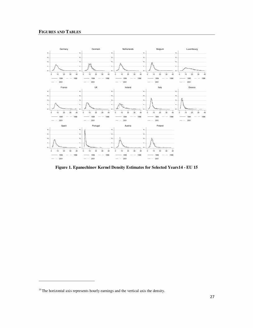
This section presents the changing shape of the cross-sectional distribution of earnings for
men over time. Figure 1 illustrates the frequency density estimates for the first wave9, 1998
and 2001 earnings distributions and Table 2 illustrates the evolution of the other moments of
the earnings distribution over time. The evolution of mean net hourly wage shows that men in
most countries got richer over time, except for Austria. Net hourly earnings became more
dispersed in most countries, except for Austria, France and Denmark.
7 The multiplicative constant equals e.g. p*(Population above 16/Sample Population). The ratio p varies across
countries so that sensible samples are obtained. It ranges between 0.001-0.01. 8 Except for France, where wage is in gross amounts
9 For Luxembourg and Austria, the first wave was recorded in 1995, whereas for Finland in 1996.

8
Plotting the percentage change in mean hourly earnings between the beginning of the sample
period and 2001 at each point of the distribution for each country (Figure 2), revealed that, in
most countries, the relationship between the quantile10
rank and growth in real earnings is
negative and nearly monotonic: the higher the rank, the smaller the increase in earnings. This
shows that in most countries, over time, the situation of the low paid people improved to a
larger extent than for the better off ones. In Austria, people at the top of the distribution
experience a decrease in mean hourly wage over time, which might explain the decrease in
the overall mean.
Netherlands, Germany, Greece and Finland diverge in their pattern from the other EU
countries experiencing a higher relative increase in earnings the higher the rank. Netherlands
is the only country where men at the bottom of the income distribution recorded a
deterioration of their work pay. For these countries, the increase in the overall mean might be
the result of an increase in the earnings position of the better off individuals, not the low paid
ones.
To complete the descriptive picture of the cross-sectional earnings distribution over time, we
provide also inequality measures. Inequality indices differ with respect to their sensitivity to
income differences in different parts of the distribution. Therefore they illustrate different
sides of the earnings distribution. The year-to-year changes in earnings inequality are
captured by computing the ratio between the mean earnings in the 9th decile and the 1st
decile (Figure 3), the Gini index, the GE indices - the Theil Index (GE(1)) -, and the Atkinson
inequality index evaluated at an the aversion parameter equal to 1 (Table 3).11
The ratio between the mean earnings in the 9th decile and the 1st deciles focuses only on the
two ends of the distribution. The Gini index is most sensitive to income differences in the
middle of the distribution (more precisely, the mode). The GE with a negative parameter is
sensitive to income differences at the bottom of the distribution and the sensitivity increases
the more negative the parameter is. The GE with a positive parameter is sensitive to income
differences at the top of the distribution and it becomes more sensitive the more positive the
parameter is. For the Atkinson inequality indices, the more positive the “inequality aversion
10 100 Quantiles
11 Besides these indices, several others were computed (GE(-1); GE(0), GE(2), Atkinson evaluated at different
values of the aversion parameter) and can be provided upon request from the authors. They support the findings
shown by the reported indices.

9
parameter” is, the more sensitive the index is to income differences at the bottom of the
distribution.
The level and pattern of inequality over time as measured by the ratio between the mean
earnings in the 9th decile and the 1st decile differs to a large extent between the EU14
countries. Two clusters can be identified. The first one is comprised of Netherlands, Begium,
Italy, Finland, Austria and Denmark and is characterized by a small relative distance between
the bottom and top of the distribution. The other cluster identifies countries with a higher
level of inequality, with ratios between 2.75 and 4.
In 1994, based on the Gini index, Portugal is the most unequal, followed by Spain, France,
Ireland, UK, Greece, Germany, Italy, Belgium, Netherlands and Denmark. In general, the
other two indices confirm this ranking. However, using the Theil index, France appears to be
more unequal than Spain, whereas using the Atkinson index, Ireland appears to be more
unequal than France and as equal as Spain.
In 2001, based on the Gini index, Portugal is still the most unequal, followed by France,
Greece, Luxembourg, Spain, UK, Germany, Ireland, Netherlands, Italy, Finland, Belgium,
Austria and Denmark. In general, the other two indices confirm this ranking. Based on Theil,
however, Greece is more unequal than France, and Spain than Luxembourg. Based on
Atkinson, Luxembourg is more unequal than Greece.
For most countries, all indices show a consistent story regarding the evolution of inequality
over the sample period, except for Germany, France and Portugal, where the evolution of the
Gini, Theil and Atkinson index is opposite to the one observed for the D9/D1. Based on Gini,
Theil and Atkinson, Netherlands, Greece, Finland, Portugal, Luxembourg, Italy and Germany
recorded an increase in yearly inequality, and the rest a decrease.
The relative evolution over the sample period is captured in Figure 4, which illustrates for
each country, the change in inequality as measured by Gini, Theil, Atkinson index and the
D9/D1. Based on Gini, the highest increase in inequality was recorded by Netherlands
(around 15%), followed by Greece, Finland, Portugal, Luxembourg, Italy and Germany. The
highest decrease was recorded in Ireland (around 20%), followed by Austria, Denmark,
Belgium, Spain, France and UK. Based on the Theil index, Portugal records a higher increase
than Finland, Italy a higher increase than Luxembourg and Spain a higher decrease than

10
Belgium. Based on Atkinson index, Portugal records a higher increase than Finland and UK a
higher decrease than France.
For Netherlands, Finland and Greece the increase in the distance between the top and bottom
of the distribution and in the overall level of inequality can be explained by the improved
earnings position of the better off individuals. Hence in these countries, the economic growth
benefitted the high income people and leaded to an increase in earnings inequality.
Luxembourg and Italy recorded an increase in inequality based on all indices, but the
situation at the bottom improved to a larger extent than for the top. Thus the increase in
inequality might be the result of other forces affecting the distribution, such as mobility in the
bottom and top deciles.
For France, the relative distance between the top and the bottom 10% appears to increase
over time, in spite of a higher relative increase in mean earnings at the bottom of the
distribution compared with the top. This discrepancy could be explained by the presence of
earnings mobility in the bottom and top 10% of the earnings distribution. The improved
conditions for people in the bottom of the distributions could explain the decrease in earnings
inequality as displayed by the other three indices.
Germany records opposite trends from France: the situation of the better off individuals
improved to a larger extent than for low paid ones, which explains the increase in the overall
inequality as captured by the Gini, Theil and Atkinson indices. The evolution of the ratio
between mean earnings at the top and the bottom deciles is opposite to what was expected:
the decrease might suggest that there are other forces at work, such as mobility in the top part
of the distribution, which determined mean earnings to decrease for this group.
Portugal records similar trends with Germany, except for the negative correlation between the
rank in the earnings distribution and the growth in earnings. Thus, the fact that low paid
individuals improved their earnings position to a higher extent relative to high paid
individuals, lowering the distance between the bottom and the top deciles of the earnings
distribution did not have the expected effect of lowering overall earnings inequality as
measured by the Gini, Theil and Atkinson indices. Mobility is expected to be the factor
counteracting all these movements.
11
For the rest of the countries, the increase in the overall mean, coupled with the higher relative
increase in the earnings position of the low paid individuals compared with high earnings
individuals can be an explanation for their decrease in inequality.
Besides the direction of evolution, also the magnitude of the change records differences
among inequality indices. In general, the magnitude of the change is the highest for the index
that is most sensitive to the income differences at the top of the distribution, followed by
bottom and middle sensitive one, sign that most of the major changes happened at the top and
the bottom of the distribution. There are a few exceptions. In UK, Spain, Belgium and
Denmark the magnitude of the evolution is the highest for the bottom sensitive one, followed
by the top and middle ones.
6. LINKING EARNINGS INEQUALITY AND MOBILITY: INDIVIDUAL MOVEMENTS WITHIN THE
DISTRIBUTION OVER TIME
When analysing the change in the distribution of earnings, one has to pay attention to two
basic characteristics. First, how far apart are individuals in terms of their wage and to what
extent does the ranking of each individual change from one period to the next. Section 5
offered a broad overview of the first characteristic. This section focuses on the second one
and analyses the intra-distributional mobility of earnings over the period 1994 – 2001.
6.1.Mobility among labour market states
To understand mobility patterns over time, it is informative to inspect mobility both within
the wage distribution and into and out of the distribution to other employment states. For this
purpose, we compute the quintiles of the wage distribution and present short-term and long-
term transitions both between quintiles and to other employment states. 12
Table 4 presents one-year period transition matrices for men between the first and second
wave and between 2000 and 2001. For all countries, one-year labour market transition
matrices portray a picture of persistence, with little short-term mobility. The diagonal
elements of these matrices are much higher than the off-diagonal elements, suggesting a low
degree of mobility from one period to the next, both in terms of quintiles of the earnings
distribution and in states outside of employment. The concentration around the diagonal
12 Short-term transitions are defined as transitions from one year to the next. Long-term transitions are defined as
transitions from the first to the last wave.

12
decreases the further one moves from the diagonal, indicating that those individuals that do
change their labour market position from one period to the next, do not move very far.
In most countries, individuals in the lowest two quintiles are more likely to enter
unemployment and inactivity compared with the rest of the distribution. Netherlands is an
exception, where the top and the bottom of the distribution have similar high rates of entering
unemployment and inactivity. Similarly, those unemployed and inactive that managed to get
a job in the next period are more likely to enter the lower quintiles of the distribution. These
findings are consistent with previous findings, for example Dickens (2000) for UK over the
period 1975-1994.
In the beginning of the sample period, the highest short-term persistence in unemployment
was recorded in Ireland, Luxembourg, Italy, Finland, Belgium and Austria where between
62.45% and 50.63% kept their status from one year to the next, followed by Spain and
Netherlands with 46% and 42.92%, and Germany, UK, Greece, Portugal, France and
Denmark with rates between 39.42% and 34%. The highest persistency in inactivity was
recorded in France, Belgium, Ireland and Portugal where more than half kept the same status
in 1995. Over time, short-term mobility out of unemployment increased in Luxembourg,
Ireland, Italy, Spain, Portugal, Austria and Finland, whereas short-term mobility out of
inactivity increased only in Belgium, France and UK.
Looking at the pattern of mobility over a longer time span (Table 5), mobility measured over
the whole sample period is higher than one-period mobility: the concentration along the
diagonal is much less than when measured over one year. These trends are consistent with
previous findings. (Atkinson et al., 1992; OECD, 1996; Dickens, 1999) The highest long-
term persistency in unemployment is found in Belgium, UK, Italy, Germany and Spain,
where between 23% and 12% maintained their status in 2001. The highest persistency in
inactivity is in France, Belgium, Portugal, Spain, Netherlands and Ireland with rates between
29% and 23%.
6.2.The transition matrix approach to mobility among income quintiles
Having introduced the general picture of mobility between different labour market states, the
next step is to explore short and long-term mobility between income classes, as well as how
short-term earnings mobility patterns changed over time.

13
Short-term earnings transition matrices (Table 6) portray a picture of persistence, with little
mobility over a one-year period: the diagonal elements of these matrices are much higher
than the off-diagonal elements. All rows display high predictability and origin dependence
(the transition probabilities are not equal) meaning that the position in the earnings
distribution the next period depends heavily on the initial state. The concentration around the
diagonal decreases the further one moves from the diagonal, indicating that those individuals
that do change their income position from one period to the next, do not move very far. For
all countries, short-term persistency appears to be the highest for the top quintile, followed by
the bottom and middle ones.
Of those in the lowest quintile in the first wave, the highest percentage of people that were
still in the lowest quintile one year later is recorded in Luxembourg (76.59%), followed by
Germany (71.28%), Italy, France, Finland, Netherlands and Ireland, with values between
60% and 70%, and Portugal, Austria, UK, Denmark, Spain, Belgium and Greece, with values
between 50% and 60%.
For the middle quintile, in the first wave, the highest mobility is observed in Austria, where
27.53% maintained their state from one year to the next, followed by Denmark (32.22%),
Greece, Finland, Spain, Italy, Belgium, Ireland and Germany with a persistency between 40%
and 50%, France, UK and Portugal with values between 50% and 55%, and finally
Luxembourg, where 68.15% of those in the middle quintile in the first wave maintained their
earnings position until the next period.
For the top quintile, Portugal, followed by Germany, UK, Netherlands, Ireland, Spain record
the highest persistency in the first wave, with a probability of over 80% of remaining in the
same state one year later. Next follow Luxembourg, Belgium, Italy, France and Finland, with
a probability between 80% and 70%, Austria, Denmark and Greece, with a probability
between 70% and 60%.
Over time, short-term income mobility for individuals belonging to the first quintile
decreased in all countries, with three exceptions: Luxembourg, Spain and Finland. Middle
quintiles recorded a decrease in short-term mobility, except for UK, Belgium, and Ireland
which did not change in mobility. Short-term mobility increased for the top quintile in
Germany, Netherlands, Ireland, Spain and Portugal, and decreased in the rest. A decrease in
short-term mobility over time suggests that in 2000-2001, low paid individuals find more

14
difficult to move up the income distribution compared with the first two waves. For the
middle quintile, mobility increased only in Belgium, UK and Portugal.
In 2000-2001, for the bottom quintile the highest persistency was recorded in Portugal,
Germany, Austria, Belgium, Netherlands and Luxembourg where between 78% and 70%
remained in the same income group, followed by Greece, France, Ireland, Denmark with
probabilities between 69% and 60%, and UK, Finland, Italy and Spain with rates between
59% and 49%. For the middle quintile, the persistency is high in Luxembourg, Greece,
Portugal, France, Austria, UK, Germany, Italy, and Netherlands with rates between 68% and
50%, and the rest with rates between 47% (Spain) and 32% (Denmark). For the top quintile,
all countries have a high persistency: between 87% (Luxembourg) and 73% (Finland)
remained in the same earnings group.
As expected, for most countries and most income quintiles, long-term mobility (Table 7)
appears to be higher compared with short-term mobility, but the persistency is still very high.
The concentration along the diagonal is less than when measured over just one year.
For those in the bottom quintile in the first wave, the degree of long-term persistency is the
highest in Germany, Austria, Finland, Portugal and France, where between 49% and 41%
remained in the same earnings quintile in 2001, followed by Luxembourg, Netherlands,
Spain, Belgium, Italy, Denmark, UK, Greece and Ireland, with values between 40% and 23%
The mobility of the bottom quintile is higher than mobility of the middle quintile in Denmark,
Luxembourg, UK, Ireland and Greece. From those in the middle quintile in the first wave,
between 21% (Austria) and 45% (Luxembourg) are still in the middle quintile in the last
wave. For those in the top quintile, the persistency is much higher, ranging between 88% and
and 71% for Spain, Luxembourg, Portugal, Netherlands, Ireland, Germany, UK and Italy, and
between 69% and 57% for Belgium, France, Finland, Austria, Greece and Denmark.
The decreasing degree of persistence with the time span is consistent with previous research
which proved that the transitory component of earnings dies off after a certain number of
years. The effects of the transitory shocks which might have affected earnings in one year are
expected to diminish with time, determining people that experienced the transitory shocks to
regain their pre-shock position in the earnings distribution. Exceptions from this trend are
observed for the top quintile in Luxembourg and Greece, where long-term mobility is roughly
equal to short-term mobility, suggesting the existence of high permanent differences between

15
individual earnings, and in Spain, where long-term mobility decreased compared to short-
term mobility.
The information in the transition matrices can be summarized by the immobility ratio and the
average jump. Figure 5, Figure 6 and Table 8 illustrate short and long-term immobility ratios
and average jump (AJ) for the earnings quintiles transition matrices, both in absolute values
and relative to the case of perfect mobility. For the interpretation, we use the ones relative to
the case of perfect mobility.
Short-term immobility ratios for all countries over time (Figure 5) have values between 1.6
and 1.9 times the immobility ratio for the case of perfect mobility, suggesting a very high
degree of persistency on or close the diagonal from one year to the next. In the first wave,
Greece has the lowest persistency, followed by Austria, Belgium, Denmark, Italy and
Finland, and, at a higher level, by Spain, France, Portugal, Ireland, UK, Germany,
Netherlands and Luxembourg.
Short-term average jump over time (Figure 6) records values between 0.15 and 0.4 of the
value under perfect mobility, suggesting a low to moderate degree of mobility outside the
diagonal for all countries. In the first wave, the lowest average jump is recorded in
Luxembourg (above 0.2), followed by Germany, Portugal and Netherlands (with values close
to 0.3), UK, France, Ireland, Spain, Italy, Finland, Belgium and Denmark (with values
between 0.3 and 0.4), and Austria and Greece (with values greater than 0.4).
As illustrated in Figure 5 and Figure 6, some countries recorded a decrease and others an
increase in short-term mobility over time. In general, over time, the evolution of the
immobility ratio appears to be negatively associated with the evolution of the average jump:
the larger the increase in mobility on and close to the diagonal (decrease in immobility ratio),
the larger the increase in mobility away from the diagonal (increase in average jump) and
vice versa.
Greece, Austria, Belgium, France, Italy, Portugal, Germany, Luxembourg and Finland
recorded a decrease in mobility close to the diagonal (increase in the immobility ratio) and a
decrease in mobility away from the diagonal (decrease in the average jump). The magnitude
of the evolution is the highest in the first five countries, ranging between 9% and 3% for the
immobility ration, and 41% and 18% for the AJ. The relative decrease in mobility as
measured by AJ is higher than the relative decrease in mobility as measured by the

16
immobility ratio, suggesting that the off-diagonal short-term mobility increased to a higher
extent than the mobility along the diagonal. An exception is Finland, where the reverse holds.
Spain has the largest increase in mobility close or on the diagonal (a decrease of 4% in
immobility ratio) and the largest increase in mobility away from the diagonal (16.8%). In the
same category are situated also Ireland and UK, but with a lower magnitude of the evolution
(around 0.3%-1% for the immobility ratio and 3%-4% for AJ). Except Spain, the increase in
the average jump is higher than the decrease in the immobility ratio.
Denmark and Netherlands represent an exception from this rule, recording both a decrease in
immobility ratio and a decrease in the average jump, therefore an increase in mobility on the
diagonal and a decrease in mobility away from the diagonal. Moreover, the decrease in off-
diagonal mobility (11% for Netherlands and 5% for Denmark) is greater than the decrease of
mobility on or close to the diagonal (0.4% in Netherlands and 0.8% in Denmark).
Mobility close to the diagonal appears to converge over time in five clusters: first,
Luxembourg which records the highest immobility ratio in 2000-2001; second, Germany,
France and Greece; third, UK, Belgium, Netherlands, Portugal, Italy and Austria; forth,
Ireland and Finland, and lastly, with the lowest immobility ratio, Denmark and Spain.
Similarly, mobility away from the diagonal appears to converge over time in four clusters:
first, Luxembourg – the lowest average jump in 2000-2001; second, Germany, France,
Austria, Netherlands, Belgium and Greece, Portugal; third, Italy, UK and Ireland; and lastly,
Finland, Spain and Denmark, with the highest mobility away from the diagonal in 2000-2001.
Overall, Luxembourg appears to diverge from the other EU countries.
In line with previous studies, the longer the period over which mobility is measured the
higher the mobility, both close and away from the diagonal of the earnings transition matrix.
(Table 8) Long-term immobility ratio records values between 1.4 and 1.7, whereas the
average jump in the long run is between 0.3 and 0.6, indicating a high degree of persistency
close or on the diagonal and a high mobility away from the diagonal. Based on both indices,
the lowest long-term mobility is recorded in Luxemboug13
, followed by France, Spain,
Germany, Netherlands and Portugal which record similar values. UK records a slightly higher
13 The value for Luxembourg and Austria illustrated the mobility over a period of 6 years, and for Finland over 5
years.

17
mobility, similar with Belgium, Italy and Greece. Denmark and Ireland record the highest
mobility in the long run, confirmed both by the immobility and the average jump.
Figure 8 illustrates the relative difference between long and short-term mobility, based on the
immobility ratio and average jump. For all countries, the longer the accounting period, the
decrease in the immobility ratio is lower than the increase in the average jump, which
suggests that mobility away from the diagonal increases to a higher extent compared with the
mobility close to the diagonal. Thus the longer the time period, the more likely it is that
people move away from their initial state.
The ranking of the countries based on the relative difference between long and short-term
mobility reveals that the relative change in the average jump with the time horizon is
negatively associated with the relative change in the immobility ratio with the time horizon.
The first six countries which record the highest drop in the immobility ratio with the time
horizon are among the first seven countries with the highest increase in the average jump. It
is the case of Denmark, Ireland, UK, Germany, Netherlands and Portugal. Denmark appears
to record the highest decrease in persistency close to the main diagonal (approximately 17%),
whereas the increase in the mobility away from the diagonal is of almost 55%. Ireland, which
has a similar decrease in the immobility ratio, has the highest increase in the average jump,
almost 90%. UK, Germany, Portugal and Netherlands record a relatively smaller reduction in
the immobility ratio (between 11% and 14%) than Denmark and Ireland and a higher increase
in the average jump (over 60%) than Denmark, but lower than Ireland.
These are followed by Italy, Spain, Finland, Belgium, Greece and France, which record a
smaller decrease in the immobility ratio (between 6% and 11%) and an increase of more than
40% in the average jump. Luxembourg records the lowest increase in mobility close to the
main diagonal and among the highest increase in mobility away from the main diagonal,
suggesting that the longer the period of time, the more likely it is that people move away
from their initial position in the earnings distribution.
In the long run, Luxembourg appears to be the least mobile, and Denmark and Ireland the
most mobile, both close to and away from the diagonal. Long-term immobility ratios are
similar for the other countries, whereas for AJ more heterogeneity is observed. Overall, we
observed less heterogeneity with respect to long-term mobility rates compared with short-
terms, suggesting that over lifetime earnings mobility rates are expected to converge to

18
similar levels in most countries. The convergence is expected to be more evident for the
immobility ratio than for AJ.
6.3.Alternative approach to mobility (Dickens 1997, 2000)
Similar to the transition matrix approach, we look first at short-term mobility and then at
long-term mobility. Figure 10 presents plots of percentile rankings of male earnings in
1994/1995 and 2000/2001, and. Figure 11 percentile plots for 1994/1995 and 1994/2001.
For the pair of years situated at 1 year time horizon a high earnings persistency is observed
for all countries: most of the individuals are concentrated in a band around the 45-degree line,
at different degrees across countries. The highest concentration is observed at the two
extremes of the distribution, meaning that individuals situated at the bottom and top of the
earnings distribution have a lower mobility compared to the ones in the middle of the
distribution, which is in line with the findings from the transition matrix approach.
In the beginning of the sample period, the countries with the lowest overall short-term
mobility (highest concentration along the 45-degree line) appear to be Germany, Netherlands,
Luxembourg, France, UK, Ireland, Italy, Spain and Portugal. The most mobile appears to be
Greece.
In order to understand better how the pattern of mobility changed over time we look at pairs
of earnings rankings situated at the same time horizon (Figure 10). The concentration along
the 45-degree line appears to increase over time, suggesting a decreasing degree of mobility
from one year to the next, for most countries. Denmark, Ireland, Spain represent an
exception, recording an apparent diminishing concentration along the 45-degree line and
therefore an increase in mobility.
If one looks at the different parts of the distribution, diverging patterns appear. For those at
the bottom of the distribution, mobility appears to increase in Denmark, Ireland, Spain and
Finland, whereas for the other countries a higher concentration can be observed over time.
These findings are in line with the ones from the transition matrix approach, except for
Denmark, Ireland and Luxembourg, where the reversed in observed.
The concentration in the middle of the distribution increased over time, suggesting a
decreasing degree of mobility from one year to the next, for most countries. Exceptions are
Denmark, Belgium, UK, Ireland and Spain, where people situated in middle part of the
19
distribution appear to become more mobile over time. Except for Denmark, Belgium, Ireland
and Spain, these findings are confirmed also by the transition matrix approach.
In the top of the distribution, mobility appears to increase in Germany, Denmark,
Netherlands, Belgium and Ireland. Except for Denmark, Belgium, Spain and Portugal, these
results are confirmed also by the transition matrix approach.
These differences observed between the two approached can be explained by the main
limitation of the transition matrix approach: it fails to capture the movement within each
earnings quintile, and thus underestimates the true degree of mobility.
There are a few individuals that record a huge jump in their rank from one year to the next:
some that start at the bottom and jump to the top in the next period, and vice versa. This
indicates the presence of a limited measurement error in hourly earnings in all countries.
Looking at mobility across different time horizons (Figure 11), we observe that the longer the
time span between the pair of earnings rankings, the less concentrated the scatter becomes
along the 45-degree line, suggesting an increase in mobility with the time span. This trend is
valid for all years and for all countries, and reconfirms previous findings.
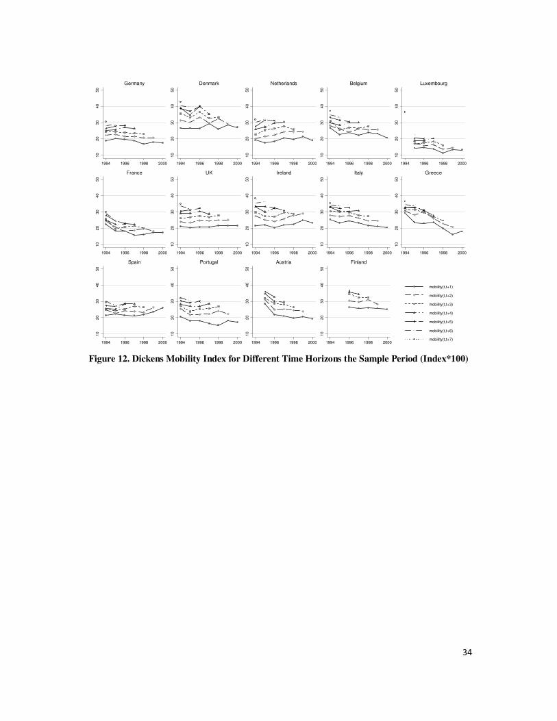
The information in the rank scatter plots is summarised by the mobility index in (0.2). Figure
12 and Table 9 illustrate the evolution of the mobility index in (0.2) for different time
horizons over the sample period for all countries. The values from all time horizons are below
the value expected if earnings were independent in both years.
Figure 13 illustrates the evolution of short-term mobility over time for all countries. Short-
term mobility in the beginning of the sample period was the highest in Greece, followed by
Austria, Belgium, Denmark and Finland with values over 0.25. Next follows Italy, France,
Spain, Ireland, UK and Portugal with values between 0.2 and 0.25. The lowest mobility is
recorded in Luxembourg, Germany and Netherlands, which record values lower than 0.2.
This ranking is in general confirmed by the ranking based on the immobility ratio and the
average jump.
The evolution of short-term mobility over time differs across countries. Except Spain,
Ireland, UK and Denmark, all other countries record a decrease in the degree of mobility
from one year to the next, which is in general consistent with the evolution of the immobility
ratio and average jump. Denmark and Netherlands are exceptions, recording opposite trends
in mobility close and away from the diagonal.

20
These mobility trends correspond to years 1994 to 2000. Therefore, linking with the
evolution of inequality over 1994 and 2000 (Table 3), we conclude that in 2000 men were:
better off both in terms of their relative wage and opportunity to escape low pay in the next
period in Denmark, UK, Ireland, and Spain; better off in terms of their relative wage, but
worst off in terms of their chance to escape low pay in Belgium, France, Austria and Finland;
and worst off in terms of both in Netherlands, Luxembourg, Italy, Greece and Portugal.
In 2000-2001 a convergence in mobility rates is observed for four country clusters.
Luxembourg, which records the lowest mobility, and Denmark, which record the highest
mobility, have a singular evolution. Spain and Finland appear to converge towards a lower
mobility than Denmark, followed by Ireland, which also has a singular evolution. The next
cluster in terms of mobility is formed by UK, Italy and Belgium. The last two clusters are
Austria and Netherlands, and Greece, Portugal, France and Germany. This ranking is in
general confirmed by the ranking based on the immobility ratio and the average jump.
Figure 14 summarizes the relative change in short-term mobility for all countries. The highest
decrease in mobility is recorded by Greece, with a reduction of almost 40%, followed by
Austria, with a reduction of more than 30%, Belgium and France over 20%, Italy and
Portugal between 15% and 20%, and Luxembourg, Germany, Finland and Netherlands with a
reduction lower than 10%. Spain records the highest increase in short-term mobility with a
rate of over 20%, followed by Ireland, UK and Denmark, with a rate below 10%.
The ranking, the magnitude and the direction of the relative change in short-term mobility
based on Dickens index are, in general, similar with those based on the average jump. (Figure
7 and Figure 14). A big discrepancy is observed in the direction of evolution for Denmark:
based on average jump mobility decreased with almost 10%, whereas based on Dickens index
it increases with almost 2%. Differences in the magnitude of the evolution are observed for
Netherlands, Germany, Luxembourg and Finland, where the increase in mobility was higher
as measured by the average jump than by the Dickens index.
The difference in the ranking, magnitude and the direction of evolution of short-term mobility
might be explained by the limitations of using quintile transition matrices to look at mobility,
particularly when looking at changes in mobility over time. If the earnings distribution has
widened over time, then the size of the quintiles has also increased, so it might be that the
movement across quintiles decreased. However, it might also be the case that mobility within
quintiles has increased, which cannot be captured by the transition matrix approach.
21
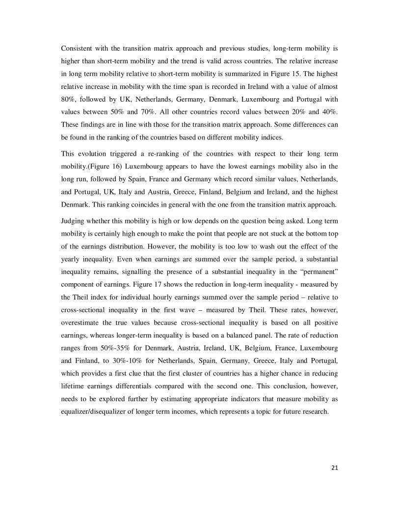
Consistent with the transition matrix approach and previous studies, long-term mobility is
higher than short-term mobility and the trend is valid across countries. The relative increase
in long term mobility relative to short-term mobility is summarized in Figure 15. The highest
relative increase in mobility with the time span is recorded in Ireland with a value of almost
80%, followed by UK, Netherlands, Germany, Denmark, Luxembourg and Portugal with
values between 50% and 70%. All other countries record values between 20% and 40%.
These findings are in line with those for the transition matrix approach. Some differences can
be found in the ranking of the countries based on different mobility indices.
This evolution triggered a re-ranking of the countries with respect to their long term
mobility.(Figure 16) Luxembourg appears to have the lowest earnings mobility also in the
long run, followed by Spain, France and Germany which record similar values, Netherlands,
and Portugal, UK, Italy and Austria, Greece, Finland, Belgium and Ireland, and the highest
Denmark. This ranking coincides in general with the one from the transition matrix approach.
Judging whether this mobility is high or low depends on the question being asked. Long term
mobility is certainly high enough to make the point that people are not stuck at the bottom top
of the earnings distribution. However, the mobility is too low to wash out the effect of the
yearly inequality. Even when earnings are summed over the sample period, a substantial
inequality remains, signalling the presence of a substantial inequality in the “permanent”
component of earnings. Figure 17 shows the reduction in long-term inequality - measured by
the Theil index for individual hourly earnings summed over the sample period – relative to
cross-sectional inequality in the first wave – measured by Theil. These rates, however,
overestimate the true values because cross-sectional inequality is based on all positive
earnings, whereas longer-term inequality is based on a balanced panel. The rate of reduction
ranges from 50%-35% for Denmark, Austria, Ireland, UK, Belgium, France, Luxembourg
and Finland, to 30%-10% for Netherlands, Spain, Germany, Greece, Italy and Portugal,
which provides a first clue that the first cluster of countries has a higher chance in reducing
lifetime earnings differentials compared with the second one. This conclusion, however,
needs to be explored further by estimating appropriate indicators that measure mobility as
equalizer/disequalizer of longer term incomes, which represents a topic for future research.

22
7. LINKING MOBILITY AND INEQUALITY
Next we aim to link the patterns in short and long-term mobility with yearly inequality. This
requires a backward looking approach. In interpreting the figures one has to pay attention to
the difference in samples in computing inequality and mobility. The inequality measures are
based on all individuals with positive earnings. The mobility measures refer to balanced 2-
year panels, meaning individuals that recorded positive earnings in both years. We chose
using an unbalanced panel for inequality to avoid underestimating the degree of dispersion.
When interpreting the results, however, we have to bear in mind that the degree of inequality
in period t depends also on the inflows and outflows of the sample in period t, not only on the
degree of mobility from one period.
7.1.Short-Term Mobility and Yearly Inequality
Inequality in time t depends on inequality in time t-1, mobility between t and t-1 and
individuals entering and exiting the sample between period t-1 and t. Thus inequality in 1995
depends on inequality in 1994 and mobility between 1994 and 1995. Similarly, inequality in
2001 depends on inequality in 2000 and mobility between 2000 and 2001.
To shed some light on the potential link between short-term mobility and yearly inequality
we look comparatively at the evolution of short term mobility from 1994/1995 to 2000/2001
and yearly inequality between 1995 and 2001. Figure 18 – left panel - ranks the countries
with respect to their inequality in 1995 and mobility between 1994 and 1995. The same is
done in the right panel for inequality in 2001 and mobility in 2000-2001
On average, it appears that the higher the inequality in year t, the lower the mobility between
year t-1 and t. The ranking, however, has also some exceptions. For example, in 1995, Greece
has among the highest mobility levels and the highest inequality. In 2001, Spain has among
the highest mobility and among the highest inequality.
Looking at the relative change in inequality and mobility the picture is not clear-cut. Most
countries recording a decrease in mobility, record also an increase in inequality. Exceptions
are Austria and France, where both decrease. All countries recording an increase in mobility,
record a decrease in inequality between the 2nd wave and 2001. The ranking is ambiguous.
The countries with the smallest (Netherlands) and the largest (Greece) reduction in mobility
have the highest increase in inequality. Similarly, the countries with the lowest (UK) and the

23
largest (Spain) increase in mobility do not have the largest reduction in inequality. Overall, it
appears that short-term mobility has a reducing effect on yearly inequality.
7.2.Long-Term Mobility and Yearly Inequality
Similarly, extending the time frame, inequality in time t depends on inequality in time t-s and
mobility between t and t-s. Figure 20 ranks the 14 countries in terms of their long term
mobility displaying at the same time the cross-sectional inequality in 2001 and the relative
change in cross-sectional inequality between the 1st wave and 2001 for each country.
On average it appears that a higher long-term mobility is associated with a lowed cross-
sectional inequality in 2001, but the ranking in the two measures is not consistent. The
highest long-term mobility is present in Denmark, which record also the lowest inequality in
2001, but the highest inequality (Portugal) does not have the lowest mobility.
The link between long-term mobility and the relative change in inequality is ambiguous.
Mobility rates are similar, but the relative change in inequality is very heterogeneous, with no
visible pattern.
8. CONCLUDING REMARKS
In this paper we have explored wage mobility for males across 14 EU countries between
1994 and 2001 using ECHP.
Starting with the transition matrices among labour market states, we find considerable levels
of short-term immobility in all countries, with high shares of individuals staying in the same
earnings quintile from one period to the next. Individuals situated in the bottom of the
distribution are more likely to enter unemployment and inactivity compared with the rest of
the distribution. Moreover, those that manage to get a job in the next period are more likely to
be in the bottom of the earnings distribution.
Mobility over the sample period is higher than one-period mobility, suggesting that the longer
the period, the higher the opportunity to escape the initial state. The highest persistency in
unemployment is found in Belgium, UK, Italy, Germany and Spain, and in inactivity in
France, Belgium, Spain, Netherlands and Ireland.
Looking only at transition matrices among income quintiles, we found a high level of
persistency from one period to the next in all countries. Moreover, individuals that change
their income position from one period to the next do not move very far. Individuals situated

24
at the top of the distribution are less mobile than people at the bottom, which in turn are less
mobile than the middle of the distribution.
Over time, short-term mobility for the bottom quintile decreased in all countries, except
Luxembourg, Spain and Finland. In 2000-2001 the highest persistency for low-earnings
individuals is in Portugal, Germany, Austria, Belgium, Netherlands and Luxembourg where
between 78% and 70% remained in the same income group, followed by Greece, France,
Ireland, Denmark with probabilities between 69% and 60%, and UK, Finland, Italy and Spain
with rates between 59% and 49%.
Long-term mobility is higher than short-term mobility, but the persistency is still high: in
Germany, Austria, Finland, Portugal and France, between 49% and 41% remained in bottom
quintile in 2001, followed by Luxembourg, Netherlands, Spain, Belgium, Italy, Denmark,
UK, Greece and Ireland, with values between 40% and 23%. Overall, the lowest long-term
mobility close and far away from the initial state was recorded in Luxembourg, France,
Spain, Germany, Netherlands and Portugal, and the highest in Denmark and Ireland.
Most countries that recorded an increase in inequality between 1994 and 2001, recorded also
an increase in short-term persistency over time, supported both by the increase in the share of
individuals maintaining theirs state or moving to the closest state from one period to the next
and by the decrease in mobility far away from the initial state. Netherlands is an exception,
recording a decrease in the share of individuals maintaining their state or moving in the
immediate income group and a decrease in mobility very far away from the initial from the
initial state.
The decrease in inequality was accompanied by an increase in mobility close to the initial
state and a decrease in mobility very far away from the initial state in Spain, Ireland and UK,
and by the opposite in Belgium, France and Austria. In Denmark, the decrease in inequality
was accompanied by an increase in mobility close the initial state and a decrease in mobility
very far from the initial state, which might signal smaller transitory differentials compared
with the other countries.
Mobility close to the diagonal appears to converge over time in five clusters: first,
Luxembourg which records the highest IR in 2001; second, Germany, France and Greece;
third, UK, Belgium, Netherlands, Portugal, Italy and Austria; forth, Ireland and Finland, and
lastly, with the lowest immobility ratio, Denmark and Spain. Similarly, mobility away from
25
the diagonal appears to converge over time in four clusters: first, Luxembourg – the lowest
average jump in 2001; second, Germany, France, Austria, Netherlands, Belgium and Greece,
Portugal; third, Italy, UK and Ireland; and lastly, Finland, Spain and Denmark, with the
highest mobility away from the diagonal in 2001. Overall, Luxembourg appears to diverge
from the other EU countries.
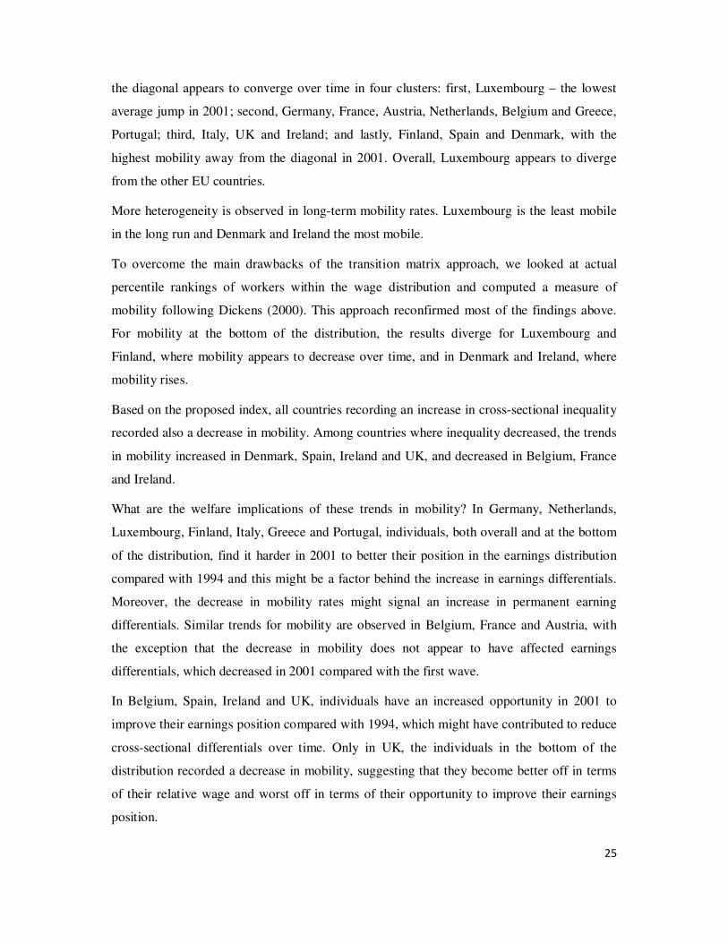
More heterogeneity is observed in long-term mobility rates. Luxembourg is the least mobile
in the long run and Denmark and Ireland the most mobile.
To overcome the main drawbacks of the transition matrix approach, we looked at actual
percentile rankings of workers within the wage distribution and computed a measure of
mobility following Dickens (2000). This approach reconfirmed most of the findings above.
For mobility at the bottom of the distribution, the results diverge for Luxembourg and
Finland, where mobility appears to decrease over time, and in Denmark and Ireland, where
mobility rises.
Based on the proposed index, all countries recording an increase in cross-sectional inequality
recorded also a decrease in mobility. Among countries where inequality decreased, the trends
in mobility increased in Denmark, Spain, Ireland and UK, and decreased in Belgium, France
and Ireland.
What are the welfare implications of these trends in mobility? In Germany, Netherlands,
Luxembourg, Finland, Italy, Greece and Portugal, individuals, both overall and at the bottom
of the distribution, find it harder in 2001 to better their position in the earnings distribution
compared with 1994 and this might be a factor behind the increase in earnings differentials.
Moreover, the decrease in mobility rates might signal an increase in permanent earning
differentials. Similar trends for mobility are observed in Belgium, France and Austria, with
the exception that the decrease in mobility does not appear to have affected earnings
differentials, which decreased in 2001 compared with the first wave.
In Belgium, Spain, Ireland and UK, individuals have an increased opportunity in 2001 to
improve their earnings position compared with 1994, which might have contributed to reduce
cross-sectional differentials over time. Only in UK, the individuals in the bottom of the
distribution recorded a decrease in mobility, suggesting that they become better off in terms
of their relative wage and worst off in terms of their opportunity to improve their earnings
position.

26
Mobility rates appear to converge towards 2001 in four country clusters. Luxembourg, with
the lowest mobility in 2001, and Denmark, with the highest mobility, have a singular
evolution. Spain and Finland appear to converge towards a lower mobility than Denmark,
followed by Ireland, which also has a singular evolution. Next, UK, Italy and Belgium
converge towards a lower level than Ireland. The last two clusters are Austria and
Netherlands, and Greece, Portugal, France and Germany. This ranking is in general
confirmed by the ranking based on the immobility ratio and the average jump.
The lowest opportunity of improving the earnings position in the long run is found in
Luxembourg followed by the four clusters which record similar values: first, Spain, France
and Germany; second, Netherlands, and Portugal; third, UK, Italy and Austria; forth Greece,
Finland, Belgium and Ireland. Finally, men in Denmark have the highest opportunity of
improving their income position in the long run. A topic for further research is to explore the
implications of the lone term mobility rates for lifetime inequality.
27
FIGURES AND TABLES
Figure 1. Epanechinov Kernel Density Estimates for Selected Years14 - EU 15
14 The horizontal axis represents hourly earnings and the vertical axis the density.
0.1
.2.3
.4
0 10 20 30 40
1994 1998
2001
Germany
0.1
.2.3
.4
0 10 20 30 40
1994 1998
2001
Denmark
0.1
.2.3
.4
0 10 20 30 40
1994 1998
2001
Netherlands
0.1
.2.3
.4
0 10 20 30 40
1994 1998
2001
Belgium
0.1
.2.3
.4
0 10 20 30 40
1995 1998
2001
Luxembourg0
.1.2
.3.4
0 10 20 30 40
1994 1998
2001
France
0.1
.2.3
.4
0 10 20 30 40
1994 1998
2001
UK
0.1
.2.3
.40 10 20 30 40
1994 1998
2001
Ireland
0.1
.2.3
.4
0 10 20 30 40
1994 1998
2001
Italy
0.1
.2.3
.4
0 10 20 30 40
1994 1998
2001
Greece
0.1
.2.3
.4
0 10 20 30 40
1994 1998
2001
Spain
0.1
.2.3
.4
0 10 20 30 40
1994 1998
2001
Portugal
0.1
.2.3
.4
0 10 20 30 40
1995 1998
2001
Austria
0.1
.2.3
.4
0 10 20 30 40
1996 1998
2001
Finland

28
Figure 2. Percentage Change in Mean Hourly Earnings by Percentiles Over The Sample Period
Figure 3. Ratio between Mean Earnings at the 9th Decile and the 1st Decile
-20
02
04
06
0
10 20 30 40 50 60 70 80 90
Germany Netherlands Belgium
Luxembourg
-20
02
04
06
0
10 20 30 40 50 60 70 80 90
France Austria UK
Ireland Finland Denmark
-20
02
04
06
0
10 20 30 40 50 60 70 80 90
Italy Spain Portugal
Greece
22
.53
3.5
4
Me
an
Ea
rnin
gs 9
th D
ecile
/1st
De
cile
1994 1995 1996 1997 1998 1999 2000 2001
Germany Netherlands
Belgium Luxembourg
France UK
Ireland
22
.53
3.5
4
Me
an
Ea
rnin
gs 9
th D
ecile
/1st
De
cile
1994 1995 1996 1997 1998 1999 2000 2001
Italy Spain
Portugal Greece
Austria Finland
Denmark

29
Figure 4. Relative Change in Inequality over Time – Gini, Theil, Atkinson(1), D9/D115
Figure 5. Immobility Ratio for One-Year Transitions between Earnings Quintiles over Time
15 Countries are ranked based on Gini index.
-50
-40
-30
-20
-10
0
10
20
30
40
Gini
Theil
A(1)
D9/D1
1.6
51
.71
.75
1.8
1.8
51
.9
Imm
ob
ility
Ra
tio
1994
-199
5
1995
-199
6
1996
-199
7
1997
-199
8
1998
-199
9
1999
-200
0
2000
-200
1
Germany France
Greece Denmark
Spain Ireland
Finland
1.6
51
.71
.75
1.8
1.8
51
.9
Imm
ob
ility
Ra
tio
1994
-199
5
1995
-199
6
1996
-199
7
1997
-199
8
1998
-199
9
1999
-200
0
2000
-200
1
Luxembourg UK
Belgium Netherlands
Portugal Italy
Austria

30
Figure 6. Average Jump for One-Year Transitions between Earnings Quintiles over Time
Figure 7. Relative Change over Time in Short-Term Immobility Ratio (IR) and Average Jump
(AJ)
.1.2
.3.4
.5
Ave
rag
e J
um
p
1994
-199
5
1995-
1996
1996
-199
7
1997
-199
8
1998-1
999
1999
-200
0
2000-
2001
Germany France
Greece Austria
Portugal Belgium
Netherlands.1
.2.3
.4.5
Ave
rag
e J
um
p
1994-1
995
1995
-199
6
1996
-1997
1997
-199
8
1998-
1999
1999-2
000
2000
-200
1
Luxembourg Spain
Denmark Finland
Ireland UK
Italy
-40
-20
020
Rela
tive C
hange in S
hort
Term
IR
Spa
in
Ireland
Denm
ark
Neth
erland
sUK
Portu
gal
Luxe
mbou
rg
Ger
man
y
Finland
France
Italy
Belgium
Austri
a
Gre
ece
-40
-20
020
Rela
tive C
hange in S
hort
Term
AJ
Gre
ece
Austri
a
Belg
ium
France
Italy
Por
tuga
l
Neth
erland
s
Ger
man
y
Luxem
bourg
Den
mark
Finland
Irela
nd UK
Spa
in

31
Figure 8. Relative Difference between Long and Short-term Immobility Ratio and Average
Jump
Figure 9. Short and Long Term Immobility Ratio and Average Jump
-20
-15
-10
-50
Re
lative
Diffe
ren
ce
Btw
Lo
ng
an
d S
ho
rt T
erm
IR
Den
mar
k
Irela
nd UK
Ger
man
y
Net
herla
nds
Por
tuga
lIta
ly
Spai
n
Finla
nd
Austria
Bel
gium
Gre
ece
France
Luxe
mbo
urg
02
04
06
08
01
00
Re
lative
Diffe
ren
ce
Btw
Lo
ng
an
d S
ho
rt T
erm
AJ
Austri
a
Gre
ece
Spai
n
Belgiu
m
Finla
nd
Franc
eIta
ly
Den
mar
k
Net
herla
nds
UK
Germ
any
Por
tugal
Luxe
mbo
urg
Irela
nd
0.5
11
.52
Den
mar
k
Irela
nd
Austri
aIta
ly
Gre
ece
Bel
gium U
K
Finla
nd
Portu
gal
Ger
man
y
Spain
Net
herla
nds
Franc
e
Luxe
mbo
urg
Short Term Immobility Ratio Long Term Immobility Ratio
0.2
.4.6
Luxe
mbo
urg
Franc
e
Spain
Ger
man
y
Net
herla
nds
Por
tuga
lUK
Finla
nd
Austri
aIta
ly
Bel
gium
Gre
ece
Irela
nd
Den
mar
k
Short Term Average Jump Long Term Average Jump

Figure 10. One-Year Earnings Mobility over Time
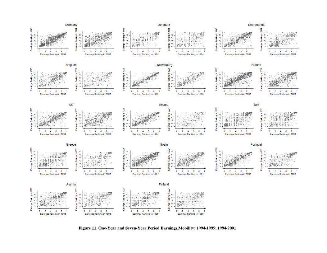
Figure 11. One-Year and Seven-Year Period Earnings Mobility: 1994-1995; 1994-2001
34
Figure 12. Dickens Mobility Index for Different Time Horizons the Sample Period (Index*100)
10
20
30
40
50
1994 1996 1998 2000
Germany
10
20
30
40
50
1994 1996 1998 2000
Denmark
10
20
30
40
50
1994 1996 1998 2000
Netherlands
10
20
30
40
50
1994 1996 1998 2000
Belgium
10
20
30
40
50
1994 1996 1998 2000
Luxembourg
10
20
30
40
50
1994 1996 1998 2000
France10
20
30
40
50
1994 1996 1998 2000
UK
10
20
30
40
50
1994 1996 1998 2000
Ireland
10
20
30
40
50
1994 1996 1998 2000
Italy
10
20
30
40
50
1994 1996 1998 2000
Greece
10
20
30
40
50
1994 1996 1998 2000
Spain
10
20
30
40
50
1994 1996 1998 2000
Portugal
10
20
30
40
50
1994 1996 1998 2000
Austria
10
20
30
40
50
1994 1996 1998 2000
Finland
mobility(t,t+1)
mobility(t,t+2)
mobility(t,t+3)
mobility(t,t+4)
mobility(t,t+5)
mobility(t,t+6)
mobility(t,t+7)

35
Figure 13. Dickens Short-Term Mobility over Time (Index*100)
Figure 14. Relative Change in Short-term Mobility Measured by the Dickens Index
10
15
20
25
30
Mo
bili
ty D
icke
ns
1994
-199
5
1995
-199
6
1996
-199
7
1997
-199
8
1998-
1999
1999-
2000
2000-
2001
Luxembourg Greece
Portugal France
Germany Austria
Netherlands
10
15
20
25
30
Mo
bili
ty D
icke
ns
1994-
1995
1995-1
996
1996-1
997
1997
-199
8
1998
-199
9
1999
-200
0
2000
-200
1
UK Belgium
Italy Ireland
Denmark Spain
Finland
-40
-20
020
Rela
tive C
hange in S
hort
Term
Incom
e M
obili
ty
Gre
ece
Austria
Belgium
Franc
eIta
ly
Portu
gal
Luxem
bourg
Ger
many
Finland
Net
herla
nds
Denm
ark
UK
Ireland
Spain
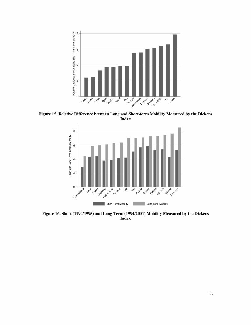
36
Figure 15. Relative Difference between Long and Short-term Mobility Measured by the Dickens
Index
Figure 16. Short (1994/1995) and Long Term (1994/2001) Mobility Measured by the Dickens
Index
020
40
60
80
Rela
tive D
iffe
rence B
tw L
ong a
nd S
hort
Term
Incom
e M
obili
ty
Gre
ece
Austri
a
Franc
e
Spain
Belgium
Finland
Italy
Portuga
l
Luxe
mbou
rg
Den
mar
k
Ger
man
y
Net
herla
nds
UK
Ireland
01
02
03
04
0
Sh
ort
an
d L
on
g T
erm
In
co
me
Mo
bility
Luxe
mbo
urg
Spa
in
Franc
e
Ger
man
y
Net
herla
nds
Por
tuga
lUK
Italy
Aus
tria
Gre
ece
Finla
nd
Bel
gium
Irela
nd
Den
mar
k
Short Term Mobility Long Term Mobility

37
Figure 17. Relative Difference between Long-Term and Cross-sectional Earnings Inequality (1st
Wave)
Figure 18. Link between Short-Term Mobility and Cross-Sectional Inequality:
Mobility (1st Wave, 2
nd Wave) -> Inequality (2
nd Wave)
Mobility (2000, 2001) -> Inequality (2001)
-50
-40
-30
-20
-10
0
Re
lative C
hange (
%)
Den
mar
k
Austria
Ireland U
K
Belgium
Fran
ce
Luxe
mbo
urg
Finlan
d
Net
herla
nds
Spain
Ger
man
y
Gre
ece
Italy
Portu
gal
010
20
30
Luxe
mbo
urg
Ger
man
y
Net
herla
nds
Por
tuga
lUK
Ireland
Spa
in
Fran
ceIta
ly
Finlan
d
Den
mar
k
Belgi
um
Aus
tria
Gre
ece
Cross-sectional Inequality (Theil) in the 2nd Wave
Mobility(1st Wave, 2nd Wave)
010
20
30
Luxe
mbo
urg
Fran
ce
Ger
man
y
Gre
ece
Net
herla
nds
Aus
tria
Italy
Belgi
um UK
Irela
nd
Finlan
d
Spa
in
Den
mar
k
Cross-sectional Inequality (Theil) in 2001
Mobility(2000, 2001)
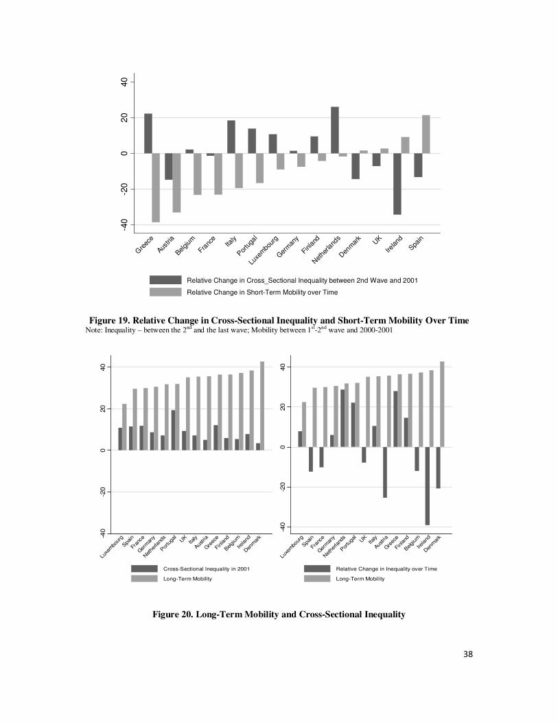
38
Figure 19. Relative Change in Cross-Sectional Inequality and Short-Term Mobility Over Time
Note: Inequality – between the 2nd and the last wave; Mobility between 1st-2nd wave and 2000-2001
Figure 20. Long-Term Mobility and Cross-Sectional Inequality
-40
-20
02
040
Gre
ece
Austria
Bel
gium
Franc
eIta
ly
Por
tuga
l
Luxe
mbou
rg
Ger
man
y
Finla
nd
Net
herland
s
Den
mar
kUK
Ireland
Spa
in
Relative Change in Cross_Sectional Inequality between 2nd Wave and 2001
Relative Change in Short-Term Mobility over Time
-40
-20
020
40
Luxe
mbo
urg
Spa
in
Fran
ce
Ger
man
y
Nethe
rland
s
Por
tuga
lUK
Italy
Austri
a
Gre
ece
Finland
Belgium
Ireland
Den
mar
k
Cross-Sectional Inequality in 2001
Long-Term Mobility
-40
-20
020
40
Luxe
mbo
urg
Spa
in
Franc
e
Ger
man
y
Nethe
rland
s
Por
tuga
lUK
Italy
Austri
a
Gre
ece
Finland
Belgium
Ireland
Den
mar
k
Relative Change in Inequality over Time
Long-Term Mobility

39
Table 1. Inflows and Outflows of Individuals in the Sample - Germany
1994 1995 1996 1997 1998 1999 2000 2001
Number of individuals with
positive earnings 25018 26059 25806 24889 23290 22955 21909 20703
Absolute number and proportion of individuals who report positive earnings in current year conditional on being in the
sample in previous year
Frequencies 23956 25224 24197 22814 22321 21290 20107
% 66.99 67.37 66.2 63.01 64.84 64.86 64.39
Absolute number and proportion of individuals who report no earnings in current year conditional on being in the sample in
the previous year
Unemployed
Inactive
Frequencies 3448 3461 4119 3932 3055 2787 2766
% 9.64 9.24 11.27 10.86 8.87 8.49 8.86
Attrition Frequencies 1885 2182 1892 3280 2951 2924 2830
% 5.27 5.83 5.18 9.06 8.57 8.91 9.06
Missing Wage Frequencies 6470 6576 6345 6180 6100 5826 5524
% 18.09 17.56 17.36 17.07 17.72 17.75 17.69
Total
Frequencies 35759 37443 36553 36206 34427 32827 31227
% 100 100 100 100 100 100 100
Table 1. Inflows and Outflows of Individuals in the Sample – Denmark
1994 1995 1996 1997 1998 1999 2000 2001
Number of individuals with
positive earnings 20899 20399 19190 19062 17321 16235 15678 15380
Absolute number and proportion of individuals who report positive earnings in current year conditional on being in the
sample in previous year
Frequencies 19854 18527 18110 16442 15334 14865 14642
% 68.74 66.59 69.43 66.23 67.41 69.6 71.6
Absolute number and proportion of individuals who report no earnings in current year conditional on being in the sample in
the previous year
Unemployed
Inactive
Frequencies 1535 1744 951 899 732 658 958
% 5.31 6.27 3.65 3.62 3.22 3.08 4.68
Attrition Frequencies 2440 3096 2914 3603 2922 2133 1775
% 8.45 11.13 11.17 14.51 12.85 9.99 8.68
Missing Wage Frequencies 5054 4454 4110 3881 3759 3703 3074
% 17.5 16.01 15.76 15.63 16.53 17.34 15.03
Total
Frequencies 28883 27821 26085 24825 22747 21359 20449
% 100 100 100 100 100 100 100
Table 1. Inflows and Outflows of Individuals in the Sample – Netherlands
1994 1995 1996 1997 1998 1999 2000 2001
Number of individuals with positive
earnings 20221 22100 22892 22753 22863 23233 24065 24130
Absolute number and proportion of individuals who report positive earnings in current year conditional on being in the
sample in previous year
Frequencies 20578 21328 21221 21055 20545 21026 21341
% 69.07 71.37 68.68 67.52 67.24 68.56 69.59
Absolute number and proportion of individuals who report no earnings in current year conditional on being in the sample in
the previous year
Unemployed
Inactive
Frequencies 2418 2356 2536 2120 1984 1840 1689
% 8.12 7.88 8.21 6.8 6.49 6 5.51
Attrition Frequencies 2941 1889 2591 3562 3984 4301 4891
% 9.87 6.32 8.39 11.42 13.04 14.02 15.95
Missing Wage Frequencies 3857 4310 4550 4448 4042 3502 2745
% 12.95 14.42 14.73 14.26 13.23 11.42 8.95
Total
Frequencies 29794 29883 30898 31185 30555 30669 30666
% 100 100 100 100 100 100 100
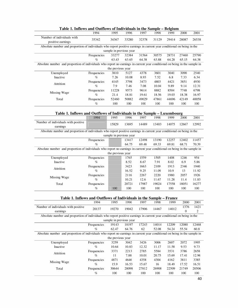
40
Table 1. Inflows and Outflows of Individuals in the Sample – Belgium
1994 1995 1996 1997 1998 1999 2000 2001
Number of individuals with
positive earnings 35342 34367 33280 32378 31129 29414 28087 26538
Absolute number and proportion of individuals who report positive earnings in current year conditional on being in the
sample in previous year
Frequencies 33277 32384 31564 30575 28731 27460 25790
% 63.43 63.65 64.38 63.88 64.28 65.15 64.38
Absolute number and proportion of individuals who report no earnings in current year conditional on being in the sample in
the previous year
Unemployed
Inactive
Frequencies 3810 5127 4378 3601 3040 3090 2540
% 7.26 10.08 8.93 7.52 6.8 7.33 6.34
Attrition Frequencies 4145 3798 3473 4803 4421 3851 4930
% 7.9 7.46 7.08 10.04 9.89 9.14 12.31
Missing Wage Frequencies 11228 9573 9614 8882 8504 7748 6798
% 21.4 18.81 19.61 18.56 19.03 18.38 16.97
Total
Frequencies 52460 50882 49029 47861 44696 42149 40058
% 100 100 100 100 100 100 100
Table 1. Inflows and Outflows of Individuals in the Sample – Luxembourg
1994 1995 1996 1997 1998 1999 2000 2001
Number of individuals with positive
earnings 15829 13695 14489 13403 14075 12667 12992
Absolute number and proportion of individuals who report positive earnings in current year conditional on being in the
sample in previous year
Frequencies
13417 12498 13190 12257 12402 11457
%
64.75 69.48 69.33 69.81 68.71 70.39
Absolute number and proportion of individuals who report no earnings in current year conditional on being in the sample in
the previous year
Unemployed
Inactive
Frequencies
1765 1559 1505 1408 1246 954
%
8.52 8.67 7.91 8.02 6.9 5.86
Attrition Frequencies
3423 1663 2109 1913 2346 1940
%
16.52 9.25 11.09 10.9 13 11.92
Missing Wage Frequencies
2116 2267 2220 1980 2057 1926
%
10.21 12.6 11.67 11.28 11.4 11.83
Total
Frequencies
20721 17987 19024 17558 18051 16277
% 100 100 100 100 100 100 100
Table 1. Inflows and Outflows of Individuals in the Sample – France
1994 1995 1996 1997 1998 1999 2000 2001
Number of individuals with positive
earnings 20137 19270 19042 17906 14467 14012
1376
0
1421
2
Absolute number and proportion of individuals who report positive earnings in current year conditional on being in the
sample in previous year
Frequencies 19143 18197 17243 14014 12209 12080 12468
% 62.47 64.76 62 52.08 54.24 55.54 60.8
Absolute number and proportion of individuals who report no earnings in current year conditional on being in the sample in
the previous year
Unemployed
Inactive
Frequencies 3259 3042 3426 3006 2607 2072 1995
% 10.64 10.83 12.32 11.17 11.58 9.53 9.73
Attrition Frequencies 3371 2213 2785 5584 3531 3786 2658
% 11 7.88 10.01 20.75 15.69 17.41 12.96
Missing Wage Frequencies 4871 4646 4358 4304 4162 3811 3385
% 15.9 16.53 15.67 16 18.49 17.52 16.51
Total
Frequencies 30644 28098 27812 26908 22509 21749 20506
% 100 100 100 100 100 100 100

41
Table 1. Inflows and Outflows of Individuals in the Sample – UK
1994 1995 1996 1997 1998 1999 2000 2001
Number of individuals with positive
earnings 24949 25329 25495 26010 26145 25750 25674 25264
Absolute number and proportion of individuals who report positive earnings in current year conditional on being in the
sample in previous year
Frequencies 24511 24848 25303 25278 25006 24881 24467
% 64.59 66.31 67.06 67.04 67.36 68.33 68.58
Absolute number and proportion of individuals who report no earnings in current year conditional on being in the sample in
the previous year
Unemployed
Inactive
Frequencies 4712 5053 4663 4140 3941 3607 3595
% 12.42 13.48 12.36 10.98 10.62 9.91 10.08
Attrition Frequencies 1836 966 1169 2073 1919 2153 2105
% 4.84 2.58 3.1 5.5 5.17 5.91 5.9
Missing Wage Frequencies 6888 6605 6597 6213 6257 5774 5510
% 18.15 17.63 17.48 16.48 16.85 15.86 15.44
Total
Frequencies 37947 37472 37732 37704 37123 36415 35677
% 100 100 100 100 100 100 100
Table 1. Inflows and Outflows of Individuals in the Sample – Ireland
1994 1995 1996 1997 1998 1999 2000 2001
Number of individuals with positive
earnings 13937 13221 12590 12515 12435 12091 10745 9727
Absolute number and proportion of individuals who report positive earnings in current year conditional on being in the
sample in previous year
Frequencies 12750 12217 12212 12020 11668 10236 9507
% 49.99 50.04 52.41 53.13 54.1 51.63 54.65
Absolute number and proportion of individuals who report no earnings in current year conditional on being in the sample in
the previous year
Unemployed
Inactive
Frequencies 4930 4723 4254 3374 2905 2185 2307
% 19.33 19.35 18.26 14.91 13.47 11.02 13.26
Attrition Frequencies 2167 2115 1600 1936 2516 3288 2362
% 8.5 8.66 6.87 8.56 11.66 16.59 13.58
Missing Wage Frequencies 5656 5359 5235 5292 4480 4116 3220
% 22.18 21.95 22.47 23.39 20.77 20.76 18.51
Total
Frequencies 25503 24414 23301 22622 21569 19825 17396
% 100 100 100 100 100 100 100
Table 1. Inflows and Outflows of Individuals in the Sample – Italy
1994 1995 1996 1997 1998 1999 2000 2001
Number of individuals with positive
earnings 32633 32236 32111 29661 28865 26993 26912 25170
Absolute number and proportion of individuals who report positive earnings in current year conditional on being in the
sample in previous year
Frequencies 30946 31028 28717 27188 25717 25348 24139
% 51.58 51.19 47.18 47.34 46.87 48.73 48.86
Absolute number and proportion of individuals who report no earnings in current year conditional on being in the sample in
the previous year
Unemployed
Inactive
Frequencies 7900 7799 7670 6627 6890 5662 5027
% 13.17 12.87 12.6 11.54 12.56 10.88 10.18
Attrition Frequencies 3175 2947 5922 6030 5941 5399 5920
% 5.29 4.86 9.73 10.5 10.83 10.38 11.98
Missing Wage Frequencies 17978 18836 18559 17585 16325 15610 14315
% 29.96 31.08 30.49 30.62 29.75 30.01 28.98
Total
Frequencies 59999 60610 60868 57430 54873 52019 49401
% 100 100 100 100 100 100 100
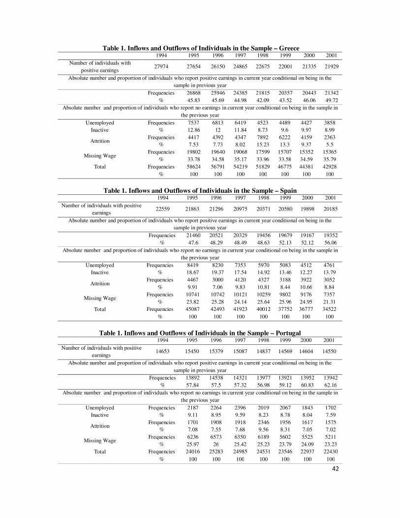
42
Table 1. Inflows and Outflows of Individuals in the Sample – Greece
1994 1995 1996 1997 1998 1999 2000 2001
Number of individuals with
positive earnings 27974 27654 26150 24865 22675 22001 21335 21929
Absolute number and proportion of individuals who report positive earnings in current year conditional on being in the
sample in previous year
Frequencies 26868 25946 24385 21815 20357 20443 21342
% 45.83 45.69 44.98 42.09 43.52 46.06 49.72
Absolute number and proportion of individuals who report no earnings in current year conditional on being in the sample in
the previous year
Unemployed
Inactive
Frequencies 7537 6813 6419 4523 4489 4427 3858
% 12.86 12 11.84 8.73 9.6 9.97 8.99
Attrition Frequencies 4417 4392 4347 7892 6222 4159 2363
% 7.53 7.73 8.02 15.23 13.3 9.37 5.5
Missing Wage Frequencies 19802 19640 19068 17599 15707 15352 15365
% 33.78 34.58 35.17 33.96 33.58 34.59 35.79
Total
Frequencies 58624 56791 54219 51829 46775 44381 42928
% 100 100 100 100 100 100 100
Table 1. Inflows and Outflows of Individuals in the Sample – Spain
1994 1995 1996 1997 1998 1999 2000 2001
Number of individuals with positive
earnings 22559 21863 21296 20975 20371 20580 19898 20185
Absolute number and proportion of individuals who report positive earnings in current year conditional on being in the
sample in previous year
Frequencies 21460 20521 20329 19456 19679 19167 19352
% 47.6 48.29 48.49 48.63 52.13 52.12 56.06
Absolute number and proportion of individuals who report no earnings in current year conditional on being in the sample in
the previous year
Unemployed
Inactive
Frequencies 8419 8230 7353 5970 5083 4512 4761
% 18.67 19.37 17.54 14.92 13.46 12.27 13.79
Attrition Frequencies 4467 3000 4120 4327 3188 3922 3052
% 9.91 7.06 9.83 10.81 8.44 10.66 8.84
Missing Wage Frequencies 10741 10742 10121 10259 9802 9176 7357
% 23.82 25.28 24.14 25.64 25.96 24.95 21.31
Total
Frequencies 45087 42493 41923 40012 37752 36777 34522
% 100 100 100 100 100 100 100
Table 1. Inflows and Outflows of Individuals in the Sample – Portugal
1994 1995 1996 1997 1998 1999 2000 2001
Number of individuals with positive
earnings 14653 15450 15379 15087 14837 14569 14604 14550
Absolute number and proportion of individuals who report positive earnings in current year conditional on being in the
sample in previous year
Frequencies 13892 14538 14321 13977 13921 13952 13942
% 57.84 57.5 57.32 56.98 59.12 60.83 62.16
Absolute number and proportion of individuals who report no earnings in current year conditional on being in the sample in
the previous year
Unemployed
Inactive
Frequencies 2187 2264 2396 2019 2067 1843 1702
% 9.11 8.95 9.59 8.23 8.78 8.04 7.59
Attrition Frequencies 1701 1908 1918 2346 1956 1617 1575
% 7.08 7.55 7.68 9.56 8.31 7.05 7.02
Missing Wage Frequencies 6236 6573 6350 6189 5602 5525 5211
% 25.97 26 25.42 25.23 23.79 24.09 23.23
Total
Frequencies 24016 25283 24985 24531 23546 22937 22430
% 100 100 100 100 100 100 100

43
Table 1. Inflows and Outflows of Individuals in the Sample – Austria
1994 1995 1996 1997 1998 1999 2000 2001
Number of individuals with
positive earnings 17944 17789 17199 16209 15162 13816 13056
Absolute number and proportion of individuals who report positive earnings in current year conditional on being in the
sample in previous year
Frequencies 16472 16384 15634 14551 13403 12601
%
67.96 68.2 67.49 67.2 66.51 68.21
Absolute number and proportion of individuals who report no earnings in current year conditional on being in the sample in
the previous year
Unemployed
Inactive
Frequencies
1209 1231 906 790 803 843
%
4.99 5.12 3.91 3.65 3.98 4.56
Attrition Frequencies
2195 2080 2435 2470 2409 1794
%
9.06 8.66 10.51 11.41 11.95 9.71
Missing Wage Frequencies 4361 4330 4189 3842 3538 3235
% 17.99 18.02 18.08 17.74 17.56 17.51
Total
Frequencies 24237 24025 23164 21653 20153 18473
%
100 100 100 100 100 100
Table 1. Inflows and Outflows of Individuals in the Sample – Finland
1996 1997 1998 1999 2000 2001
Number of individuals with
positive earnings
15811 15845 15895 15546 13329 13057
Absolute number and proportion of individuals who report positive earnings in current year conditional on being in the
sample in previous year
Frequencies
15246 15345 14753 12756 12588
%
55.95 57.2 59.29 53.83 64.16
Absolute number and proportion of individuals who report no earnings in current year conditional on being in the sample in
the previous year
Unemployed
Inactive
Frequencies
3446 2327 1657 1326 1267
%
12.65 8.67 6.66 5.6 6.46
Attrition Frequencies
1933 3219 2658 5219 1708
%
7.09 12 10.68 22.02 8.71
Missing Wage Frequencies
6623 5937 5814 4398 4057
%
24.31 22.13 23.37 18.56 20.68
Total
Frequencies
27248 26828 24882 23699 19620
%
100 100 100 100 100

44
Table 2. Sample Statistics of Hourly Earnings
Year 1994 1995 1996 1997 1998 1999 2000 2001
Germany
Mean 9.43 9.49 9.61 9.52 9.57 9.48 9.60 9.72
Median 8.65 8.68 8.78 8.84 8.70 8.65 8.75 8.82
Standard Deviation 4.00 4.17 4.09 4.01 4.39 4.32 4.39 4.37
Denmark
Mean 10.89 11.40 11.58 11.61 11.86 11.85 12.02 12.08
Median 10.36 10.76 10.96 11.14 11.46 11.36 11.77 11.50
Standard Deviation 3.23 3.31 3.52 3.54 3.13 3.31 3.43 3.20
Netherlands
Mean 9.69 9.56 9.59 9.70 10.02 9.88 10.04 9.91
Median 9.11 9.07 9.01 9.10 9.27 9.18 9.32 9.23
Standard Deviation 3.39 3.37 3.55 3.56 3.64 3.40 3.48 3.95
Belgium
Mean 8.48 8.82 8.71 8.75 8.81 8.83 8.92 9.10
Median 7.86 8.17 7.99 8.09 8.08 8.34 8.25 8.30
Standard Deviation 3.17 3.08 3.02 3.09 2.97 2.94 3.00 3.21
Luxembourg
Mean 16.18 15.81 16.73 17.39 17.15 17.22 17.10
Median 14.90 14.52 15.31 15.72 15.60 15.65 15.29
Standard Deviation 7.50 7.19 7.77 8.21 8.38 8.37 8.22
France16
Mean 10.23 9.92 9.87 10.05 10.33 10.60 10.55 10.87
Median 8.56 8.57 8.53 8.53 8.84 9.04 9.06 9.48
Standard Deviation 5.82 5.33 5.17 5.65 5.62 5.78 5.51 5.72
UK
Mean 8.16 8.11 8.22 8.34 8.68 9.01 9.21 9.68
Median 7.30 7.29 7.51 7.52 7.67 8.00 8.22 8.68
Standard Deviation 3.99 3.95 3.80 3.79 4.01 4.13 4.24 4.49
Ireland
Mean 9.30 9.54 9.76 10.02 10.43 10.84 11.69 12.44
Median 8.06 8.44 8.84 8.86 9.33 9.73 10.25 11.36
Standard Deviation 5.14 4.99 4.85 4.98 5.17 5.02 5.24 5.15
Italy
Mean 7.16 6.91 6.96 7.05 7.29 7.37 7.28 7.32
Median 6.65 6.32 6.43 6.48 6.69 6.76 6.59 6.67
Standard Deviation 2.77 2.59 2.67 2.68 3.01 3.00 2.99 3.04
Greece
Mean 4.95 5.03 5.23 5.59 5.63 5.85 5.70 5.77
Median 4.49 4.41 4.53 4.90 4.91 4.99 4.89 4.99
Standard Deviation 2.33 2.42 2.43 2.91 2.87 3.14 3.07 3.21
Spain
Mean 6.83 6.95 7.09 6.89 7.18 7.37 7.45 7.42
Median 5.86 5.82 5.92 5.72 6.04 6.15 6.29 6.33
Standard Deviation 3.81 3.86 4.00 3.92 4.06 4.15 4.07 3.87
Portugal
Mean 3.70 3.74 3.84 3.92 3.99 4.08 4.31 4.46
Median 2.92 2.82 2.98 3.03 3.05 3.08 3.29 3.34
Standard Deviation 2.34 2.45 2.54 2.65 2.81 2.82 3.16 3.33
Austria
Mean 9.08 8.33 8.37 8.49 8.55 8.55 8.54
Median 8.51 7.64 7.63 7.84 7.82 7.86 7.93
Standard Deviation 3.52 3.00 3.07 2.95 2.89 2.84 2.82
Finland
Mean 7.89 8.01 8.41 8.45 8.66 8.86
Median 7.48 7.57 7.85 7.90 8.18 7.97
Standard Deviation 2.70 2.77 2.92 2.91 2.93 3.29
16 Gross Amounts

45
Table 3. Earnings Inequality (Index*100) 1994 1995 1996 1997 1998 1999 2000 2001
Germany
Gini 22.15 22.34 22.04 21.89 22.58 22.81 22.75 22.54
Theil 8.22 8.61 8.23 8.06 8.85 8.96 8.92 8.72
A(1) 8.08 8.38 8.04 7.84 8.12 8.53 8.41 8.17
Denmark
Gini 15.76 15.26 15.52 15.21 14.24 14.68 14.94 14.05
Theil 4.22 3.92 4.23 4.15 3.37 3.73 3.83 3.35
A(1) 4.26 3.78 4.10 3.96 3.37 3.76 3.78 3.33
Netherlands
Gini 18.07 18.37 19.19 18.80 18.93 17.92 18.18 20.67
Theil 5.63 5.76 6.32 6.07 5.96 5.40 5.56 7.25
A(1) 5.56 5.77 6.33 5.90 5.65 5.18 5.44 7.08
Belgium
Gini 19.10 17.71 17.64 18.13 17.53 17.33 17.13 17.85
Theil 6.23 5.37 5.35 5.58 5.15 5.11 5.04 5.48
A(1) 5.92 4.95 5.04 5.24 4.85 4.92 4.69 5.14
Luxembourg
Gini 25.23 24.74 25.41 25.62 26.58 26.50 26.32
Theil 10.09 9.85 10.24 10.37 11.19 11.15 10.89
A(1) 9.88 10.00 10.16 10.02 10.95 11.09 10.66
France
Gini 27.62 26.47 26.26 27.23 27.28 27.41 26.83 26.49
Theil 13.21 12.04 11.63 12.88 12.58 12.65 11.94 11.87
A(1) 11.64 10.88 10.58 11.41 11.54 11.59 11.17 10.98
UK
Gini 24.26 24.22 23.35 23.36 23.54 23.25 23.35 23.51
Theil 10.08 10.01 9.20 9.05 9.24 9.08 9.16 9.29
A(1) 9.25 9.19 8.57 8.46 8.55 8.32 8.46 8.51
Ireland
Gini 27.59 26.87 25.76 25.47 25.00 23.39 22.77 21.70
Theil 12.87 11.97 11.00 10.83 10.60 9.31 8.78 7.85
A(1) 11.84 11.21 10.50 10.14 9.85 8.66 8.15 7.64
Italy
Gini 19.16 18.47 19.02 18.93 19.85 19.72 19.78 19.90
Theil 6.51 6.08 6.42 6.29 7.13 7.01 7.08 7.19
A(1) 5.99 5.58 5.91 5.78 6.41 6.30 6.33 6.39
Greece
Gini 23.62 24.37 23.80 25.55 25.66 26.98 26.51 26.37
Theil 9.51 9.97 9.44 11.23 11.09 12.20 11.93 12.17
A(1) 8.77 9.13 8.70 9.97 9.99 10.97 10.68 10.55
Spain
Gini 27.87 28.27 28.19 28.71 28.37 26.99 26.36 26.07
Theil 13.08 13.22 13.36 13.67 13.47 12.69 12.09 11.47
A(1) 11.84 12.13 11.94 12.33 12.17 11.07 10.60 10.28
Portugal
Gini 30.05 31.14 30.66 30.85 31.13 30.11 31.32 31.72
Theil 15.79 16.93 16.76 17.27 18.01 17.21 18.86 19.27
A(1) 13.23 14.16 13.80 14.05 14.37 13.55 14.60 14.92
Austria
Gini 19.49 18.34 18.34 17.39 17.07 16.72 16.85
Theil 6.67 5.84 5.90 5.27 5.10 4.93 4.97
A(1) 6.44 5.62 5.52 4.87 4.80 4.67 4.82
Finland
Gini 17.32 17.80 17.30 17.81 17.10 18.50
Theil 5.22 5.46 5.23 5.38 5.08 5.98
A(1) 4.94 5.29 4.83 5.19 4.76 5.53
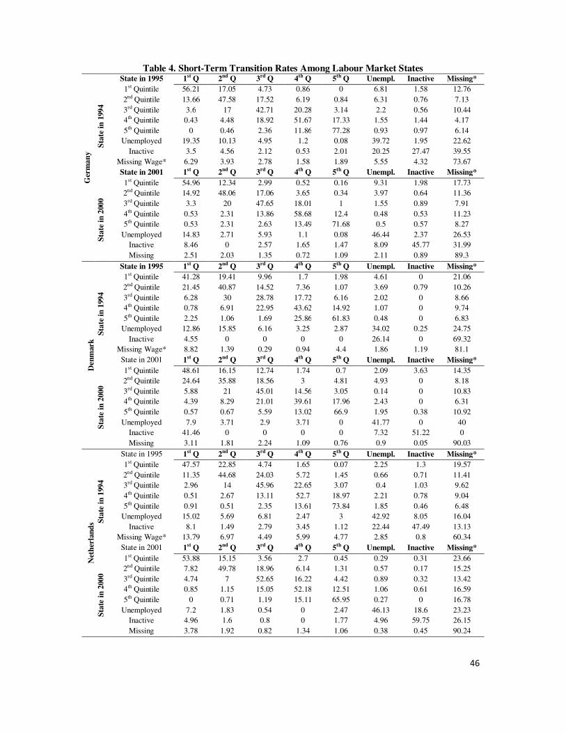
46
Table 4. Short-Term Transition Rates Among Labour Market States
Ger
ma
ny
State in 1995 1st Q 2nd Q 3rd Q 4th Q 5th Q Unempl. Inactive Missing*
Sta
te i
n 1
99
4
1st Quintile 56.21 17.05 4.73 0.86 0 6.81 1.58 12.76
2nd Quintile 13.66 47.58 17.52 6.19 0.84 6.31 0.76 7.13
3rd Quintile 3.6 17 42.71 20.28 3.14 2.2 0.56 10.44
4th Quintile 0.43 4.48 18.92 51.67 17.33 1.55 1.44 4.17
5th Quintile 0 0.46 2.36 11.86 77.28 0.93 0.97 6.14
Unemployed 19.35 10.13 4.95 1.2 0.08 39.72 1.95 22.62
Inactive 3.5 4.56 2.12 0.53 2.01 20.25 27.47 39.55
Missing Wage* 6.29 3.93 2.78 1.58 1.89 5.55 4.32 73.67
State in 2001 1st Q 2nd Q 3rd Q 4th Q 5th Q Unempl. Inactive Missing*
Sta
te i
n 2
00
0
1st Quintile 54.96 12.34 2.99 0.52 0.16 9.31 1.98 17.73
2nd Quintile 14.92 48.06 17.06 3.65 0.34 3.97 0.64 11.36
3rd Quintile 3.3 20 47.65 18.01 1 1.55 0.89 7.91
4th Quintile 0.53 2.31 13.86 58.68 12.4 0.48 0.53 11.23
5th Quintile 0.53 2.31 2.63 13.49 71.68 0.5 0.57 8.27
Unemployed 14.83 2.71 5.93 1.1 0.08 46.44 2.37 26.53
Inactive 8.46 0 2.57 1.65 1.47 8.09 45.77 31.99
Missing 2.51 2.03 1.35 0.72 1.09 2.11 0.89 89.3
Den
mark
State in 1995 1st Q 2nd Q 3rd Q 4th Q 5th Q Unempl. Inactive Missing*
Sta
te i
n 1
99
4
1st Quintile 41.28 19.41 9.96 1.7 1.98 4.61 0 21.06
2nd Quintile 21.45 40.87 14.52 7.36 1.07 3.69 0.79 10.26
3rd Quintile 6.28 30 28.78 17.72 6.16 2.02 0 8.66
4th Quintile 0.78 6.91 22.95 43.62 14.92 1.07 0 9.74
5th Quintile 2.25 1.06 1.69 25.86 61.83 0.48 0 6.83
Unemployed 12.86 15.85 6.16 3.25 2.87 34.02 0.25 24.75
Inactive 4.55 0 0 0 0 26.14 0 69.32
Missing Wage* 8.82 1.39 0.29 0.94 4.4 1.86 1.19 81.1
State in 2001 1st Q 2nd Q 3rd Q 4th Q 5th Q Unempl. Inactive Missing*
Sta
te i
n 2
00
0
1st Quintile 48.61 16.15 12.74 1.74 0.7 2.09 3.63 14.35
2nd Quintile 24.64 35.88 18.56 3 4.81 4.93 0 8.18
3rd Quintile 5.88 21 45.01 14.56 3.05 0.14 0 10.83
4th Quintile 4.39 8.29 21.01 39.61 17.96 2.43 0 6.31
5th Quintile 0.57 0.67 5.59 13.02 66.9 1.95 0.38 10.92
Unemployed 7.9 3.71 2.9 3.71 0 41.77 0 40
Inactive 41.46 0 0 0 0 7.32 51.22 0
Missing 3.11 1.81 2.24 1.09 0.76 0.9 0.05 90.03
Net
her
lan
ds
State in 1995 1st Q 2nd Q 3rd Q 4th Q 5th Q Unempl. Inactive Missing*
Sta
te i
n 1
99
4
1st Quintile 47.57 22.85 4.74 1.65 0.07 2.25 1.3 19.57
2nd Quintile 11.35 44.68 24.03 5.72 1.45 0.66 0.71 11.41
3rd Quintile 2.96 14 45.96 22.65 3.07 0.4 1.03 9.62
4th Quintile 0.51 2.67 13.11 52.7 18.97 2.21 0.78 9.04
5th Quintile 0.91 0.51 2.35 13.61 73.84 1.85 0.46 6.48
Unemployed 15.02 5.69 6.81 2.47 3 42.92 8.05 16.04
Inactive 8.1 1.49 2.79 3.45 1.12 22.44 47.49 13.13
Missing Wage* 13.79 6.97 4.49 5.99 4.77 2.85 0.8 60.34
State in 2001 1st Q 2nd Q 3rd Q 4th Q 5th Q Unempl. Inactive Missing*
Sta
te i
n 2
00
0
1st Quintile 53.88 15.15 3.56 2.7 0.45 0.29 0.31 23.66
2nd Quintile 7.82 49.78 18.96 6.14 1.31 0.57 0.17 15.25
3rd Quintile 4.74 7 52.65 16.22 4.42 0.89 0.32 13.42
4th Quintile 0.85 1.15 15.05 52.18 12.51 1.06 0.61 16.59
5th Quintile 0 0.71 1.19 15.11 65.95 0.27 0 16.78
Unemployed 7.2 1.83 0.54 0 2.47 46.13 18.6 23.23
Inactive 4.96 1.6 0.8 0 1.77 4.96 59.75 26.15
Missing 3.78 1.92 0.82 1.34 1.06 0.38 0.45 90.24

47
Table 4. (Continued)
Bel
giu
m
State in 1995 1st Q 2nd Q 3rd Q 4th Q 5th Q Unempl. Inactive Missing*
Sta
te i
n 1
99
4
1st Quintile 44.95 16.63 10.1 6.77 4.15 4.39 0.25 12.76
2nd Quintile 24.75 37.63 16.29 6.7 1.36 0.83 0 12.45
3rd Quintile 5.29 25 43.1 11.4 4 0.53 0.53 10.18
4th Quintile 3.35 5.11 21.81 45.16 15.11 0.89 0 8.57
5th Quintile 0.64 1.51 2.78 16.61 68.27 1.84 0.24 8.13
Unemployed 13.03 11.53 0 0.76 1.24 54.21 1.22 18
Inactive 0 0.81 0 0 0 13.67 64.89 20.63
Missing Wage* 6.09 2.75 1.97 0.66 0.66 2.67 0.72 84.49
State in 2001 1st Q 2nd Q 3rd Q 4th Q 5th Q Unempl. Inactive Missing*
Sta
te i
n 2
00
0
1st Quintile 62.45 15.38 7.37 0.34 0.3 0.44 0 13.72
2nd Quintile 10.49 45.04 19.82 5.54 1.73 1.71 0 15.68
3rd Quintile 5.34 17 36.25 22.99 2.37 0.97 0 15.19
4th Quintile 0.89 5.95 20.93 50.18 13.53 0.55 0 7.95
5th Quintile 0 1.3 1.6 16.38 70.82 0.45 0 9.45
Unemployed 16.9 0 2.74 0 0 58.62 0.99 20.75
Inactive 0 3.42 0 0 0 0 62.86 33.72
Missing 1.37 1.13 1.62 0.7 0.46 0.78 0.64 93.3
Lu
xem
bo
urg
State in 1996 1st Q 2nd Q 3rd Q 4th Q 5th Q Unempl. Inactive Missing*
Sta
te i
n 1
99
5
1st Quintile 57.09 14.93 1.06 0.65 0.81 3.09 0.34 22.03
2nd Quintile 12.92 54.54 14.01 0.19 0.22 1.18 0 16.92
3rd Quintile 2.36 12.16 57.08 8.76 3.39 0.58 0.36 15.31
4th Quintile 0.2 0.56 17.68 51.76 10.24 0.16 0 19.39
5th Quintile 0.25 0 3.45 14.19 65.8 0 0 16.31
Unemployed 5.3 1.32 0.55 1.54 0 59.62 2.98 28.68
Inactive 15 0 0 0 0 8 24 53
Missing Wage* 8.08 2.83 1.62 1.83 4.54 11.37 1.8 67.94
State in 2001 1st Q 2nd Q 3rd Q 4th Q 5th Q Unempl. Inactive Missing*
Sta
te i
n 2
00
0
1st Quintile 58.16 22.08 1.44 0.51 0 1.17 0 16.64
2nd Quintile 9.98 58.63 16.61 1.52 0.56 0.16 0 12.54
3rd Quintile 2.53 5.53 60.67 18.54 0.75 0 0 11.98
4th Quintile 0.28 1.26 9.48 63.97 17.43 0 0 7.59
5th Quintile 0 0.2 0.28 10.4 74.12 0 0 15.01
Unemployed 13.93 5.57 3.54 0 0 55.5 3.61 17.85
Inactive 0 0 0 0 0 9.76 66.67 23.58
Missing 0.72 0.7 0.35 0.1 0.75 0.29 0.22 96.87
Fra
nce
State in 1995 1st Q 2nd Q 3rd Q 4th Q 5th Q Unempl. Inactive Missing*
Sta
te i
n 1
99
4
1st Quintile 50.21 19.57 5.51 0.92 0.55 5.26 1.36 16.62
2nd Quintile 12.37 45.38 20.14 3.2 0.76 2.79 1.39 13.98
3rd Quintile 4.28 15 45.24 21.12 2.67 0.55 0.28 10.58
4th Quintile 2.29 4.5 14.03 48.05 19.62 0.97 0.4 10.15
5th Quintile 2.81 2.36 3.8 14.76 64.82 0.15 0.37 10.93
Unemployed 14.52 4.34 3.68 3.73 4.44 35.24 3.94 30.11
Inactive 0 0.93 3.59 0 0.93 2.66 76.1 15.8
Missing Wage* 5.16 2.62 1.82 2.96 1.95 7.24 2.55 75.71
State in 2001 1st Q 2nd Q 3rd Q 4th Q 5th Q Unempl. Inactive Missing*
Sta
te i
n 2
00
0
1st Quintile 48.37 16.06 5.75 1.99 0.54 6.84 1.09 19.36
2nd Quintile 16.79 46.58 16.86 3.13 0.29 2.88 0.44 13.04
3rd Quintile 2.14 15 49.2 16.06 0.91 1.34 0.55 14.83
4th Quintile 0.58 3.24 12.43 56.16 14.94 0.95 0.25 11.45
5th Quintile 0.44 0.18 1.53 11.03 71.68 0.18 0.18 14.78
Unemployed 16.43 8.43 2.81 1.06 0.69 49.78 1.75 19.05
Inactive 8.81 0 1.04 0 0 3.88 73.58 12.69
Missing 3.07 2.12 2.28 2.17 2.01 2.1 0.5 85.75

48
Table 4 (Continued)
UK
State in 1995 1st Q 2nd Q 3rd Q 4th Q 5th Q Unempl. Inactive Missing*
Sta
te i
n 1
99
4
1st Quintile 48.25 23.64 5.51 3.41 1.44 4.41 3.93 9.42
2nd Quintile 21.03 43.61 16.66 4.31 1.84 1.1 1.84 9.63
3rd Quintile 4.23 14 50.15 20.66 2.78 0.66 0.72 6.32
4th Quintile 0.12 3.94 17.74 53.52 14.36 1.64 2.24 6.43
5th Quintile 0.84 0.66 2.73 12.4 73.07 1.42 1.81 7.06
Unemployed 12.96 6.33 5.11 3.95 0.56 39.32 13.4 18.37
Inactive 5.29 3.75 1.37 2.37 6.87 5.58 55.45 19.32
Missing Wage* 5.37 3.51 2.11 1.64 2.15 3.77 2.9 78.56
State in 2001 1st Q 2nd Q 3rd Q 4th Q 5th Q Unempl. Inactive Missing*
Sta
te i
n 2
00
0
1st Quintile 50.79 25.43 6.02 1.86 1.84 3.59 1.36 9.11
2nd Quintile 20.73 41.53 20.23 5.79 1.87 1.58 0.39 7.88
3rd Quintile 3.9 17 47.44 17.94 2.76 1.22 1.67 7.73
4th Quintile 0.82 3.36 16.02 54.24 14.98 0.66 2.7 7.23
5th Quintile 0.57 1.85 2.71 14.07 69.86 1.81 2.73 6.4
Unemployed 11.02 1.46 2.56 1.46 2.48 63.82 1.87 15.33
Inactive 4.52 6.53 1.36 7.54 10.84 3.45 30.08 35.68
Missing 2.39 1.31 1.46 0.32 1.03 2.14 2.66 88.68
Irel
an
d
State in 1995 1st Q 2nd Q 3rd Q 4th Q 5th Q Unempl. Inactive Missing*
Sta
te i
n 1
99
4
1st Quintile 47.49 18.19 6.11 4.2 1.06 5.4 0.53 47.49
2nd Quintile 13.79 38.43 15.13 5.37 1.74 9.83 0.76 13.79
3rd Quintile 1.8 18 39.9 21.28 0.83 4.92 0 1.8
4th Quintile 0.76 3.45 20.54 41.62 18.63 1.58 0.18 0.76
5th Quintile 0 0.39 4.13 12.7 69.61 0.68 0 0
Unemployed 5.78 1.77 2.76 1.87 0.45 62.45 0.91 5.78
Inactive 3.45 0 0.19 0 0 13.98 65.33 3.45
Missing Wage* 4.14 4.32 2.71 2.22 1.09 3.1 3.01 4.14
State in 2001 1st Q 2nd Q 3rd Q 4th Q 5th Q Unempl. Inactive Missing*
Sta
te i
n 2
00
0
1st Quintile 51.96 17.6 7.85 3 0 5.91 0.6 13.07
2nd Quintile 14.37 35.77 13.25 5.43 1.59 7.12 1.87 20.6
3rd Quintile 3.63 19 39.62 14.06 3.35 2 0.37 17.64
4th Quintile 1.11 4.58 17.82 45.51 18.8 1.3 0.51 10.37
5th Quintile 0 2.95 3.04 16.48 63.81 0.37 0.56 12.78
Unemployed 7.46 4.48 2.9 1.93 1.49 58.74 7.99 15.01
Inactive 2.73 0 3.28 0 0 3.64 72.61 17.74
Missing 1.14 0.7 0.81 0.23 0.24 1.31 0.29 95.28
Ital
y
State in 1995 1st Q 2nd Q 3rd Q 4th Q 5th Q Unempl. Inactive Missing*
Sta
te i
n 1
99
4
1st Quintile 54.67 14.45 6.39 3.36 0.54 9.37 0.76 10.45
2nd Quintile 15.55 36.71 22.87 8.93 2.73 3.59 0.72 8.9
3rd Quintile 4.93 15 41.44 20.86 4.37 1.64 0.38 10.87
4th Quintile 2.88 8 14.28 45.98 18.94 1.16 0 8.77
5th Quintile 1.7 1.49 2.77 16.17 64.61 1.49 0.35 11.42
Unemployed 10.46 3.22 1.25 2.09 1.78 58.87 4.36 17.97
Inactive 3.23 3.73 0.05 2.17 0.41 8.34 33.79 48.27
Missing Wage* 4.06 1.64 0.9 0.63 1.44 6.63 1.96 82.74
State in 2001 1st Q 2nd Q 3rd Q 4th Q 5th Q Unempl. Inactive Missing*
Sta
te i
n 2
00
0
1st Quintile 54.73 14.87 4.61 2.97 1.84 2.78 1.78 16.42
2nd Quintile 12.14 44.66 19.66 3.93 1.49 1.49 0.26 16.36
3rd Quintile 2.09 18 44.44 16.3 3.33 1.22 1.04 13.73
4th Quintile 1.09 3.74 16.69 48.53 13.3 1.33 0.31 15
5th Quintile 0.36 1.89 1.95 12.32 64.9 0 0.39 18.2
Unemployed 10.09 3.41 2.3 1.61 0.39 57.96 3.48 20.77
Inactive 5.46 2.37 1.29 0.72 0 3.24 55 31.92
Missing 1.17 1.23 0.81 1.12 0.88 1.78 0.48 92.52

49
Table 4 (Continued)
Gre
ece
State in 1995 1st Q 2nd Q 3rd Q 4th Q 5th Q Unempl. Inactive Missing*
Sta
te i
n 1
99
4
1st Quintile 39.99 20.39 9.28 2.09 1.84 7.28 0.91 18.23
2nd Quintile 16.5 28.77 25.81 4.87 4.05 6.05 0.13 13.82
3rd Quintile 4.81 17 35.22 19.86 5.99 1.56 0.39 14.95
4th Quintile 2.94 6.44 20.1 36.09 18.06 2.13 0 14.24
5th Quintile 0.7 3.13 7.73 18.06 56.56 0.46 0.25 13.11
Unemployed 15.29 6.95 5.53 1.4 1.74 36.37 9.35 23.38
Inactive 6.74 2.58 0.52 0 0.63 19.07 44.73 25.73
Missing Wage* 3.68 3.03 1.79 0.92 1.5 7.48 4.83 76.77
State in 2001 1st Q 2nd Q 3rd Q 4th Q 5th Q Unempl. Inactive Missing*
Sta
te i
n 2
00
0
1st Quintile 57.69 19.5 4.41 1.08 0.37 6.24 1.19 9.51
2nd Quintile 10.75 52.41 20.83 6.52 0.82 2.18 0 6.49
3rd Quintile 4.26 14 55.8 13.9 2.45 1.59 0 7.76
4th Quintile 0 2.19 17.84 52.7 19.34 1.32 0.23 6.38
5th Quintile 0 0.5 2.58 10.8 76.59 1.57 0.95 7
Unemployed 16.89 8.83 7.46 5.7 0 39.23 9.5 12.39
Inactive 8.28 4.42 0.75 0 1.05 5.37 53.51 26.61
Missing 0.98 1.03 0.6 0.36 0.38 0.79 1.05 94.8
Sp
ain
State in 1995 1st Q 2nd Q 3rd Q 4th Q 5th Q Unempl. Inactive Missing*
Sta
te i
n 1
99
4
1st Quintile 38.99 21.45 9.27 1.57 0.18 10.95 2.06 15.55
2nd Quintile 14.17 31.82 22.21 5.62 0.78 7.95 0.71 16.74
3rd Quintile 4.64 13 33.48 20.93 2.92 8.16 0.52 16.66
4th Quintile 0.37 2.65 11.34 49.61 21.04 2.03 1.64 11.32
5th Quintile 0.4 0.24 1.22 14.67 69.13 1.94 0.33 12.06
Unemployed 13.21 8.97 7.79 2.17 0.52 46 3.27 18.06
Inactive 6.08 3.77 2.03 0.6 0.21 19.96 40.77 26.59
Missing Wage* 3.92 3.63 1.91 0.55 0.95 7.02 4.85 77.18
State in 2001 1st Q 2nd Q 3rd Q 4th Q 5th Q Unempl. Inactive Missing*
Sta
te i
n 2
00
0
1st Quintile 38.28 23.31 8.71 6.47 0.38 11.92 0.78 10.16
2nd Quintile 21.29 34.57 18.5 10.27 0.28 6.04 0.68 8.38
3rd Quintile 7.61 17 38.97 14.88 3.67 3.94 0.32 13.4
4th Quintile 3.5 4.99 18.15 40.77 16.36 2.5 1.19 12.53
5th Quintile 0 1.29 1.11 15.31 69.04 0.68 0.38 12.2
Unemployed 14.22 10.02 7.66 3.72 0.77 39.71 7.62 16.28
Inactive 2.14 0.35 0.25 0.15 0.35 10.74 68.39 17.64
Missing 2.15 1.57 0.99 1.51 1.56 1.48 1.4 89.34
Po
rtu
gal
State in 1995 1st Q 2nd Q 3rd Q 4th Q 5th Q Unempl. Inactive Missing*
Sta
te i
n 1
99
4
1st Quintile 51.15 23.41 8.84 2.5 0.17 4.76 0.2 8.97
2nd Quintile 16.63 43.8 22.63 4.26 0 2.62 0.07 9.99
3rd Quintile 5.1 12 45.81 19.03 1.86 4.21 3.72 8.14
4th Quintile 2 6.32 12.94 53.79 9.81 3.23 0.75 11.17
5th Quintile 0.03 0.21 1.72 8.8 71.88 3.85 0 13.51
Unemployed 18.83 7.45 9.93 1.79 0 36 6.41 19.59
Inactive 4.84 2.67 0.2 4.15 1.28 5.53 50.35 31
Missing Wage* 4.42 2.31 2.22 2.08 2.95 2.2 2.4 81.41
State in 2001 1st Q 2nd Q 3rd Q 4th Q 5th Q Unempl. Inactive Missing*
Sta
te i
n 2
00
0
1st Quintile 68.37 10.58 4.28 2.31 1.71 2.9 1.32 8.53
2nd Quintile 13.53 50.22 21.93 3.24 0.09 3.78 0.16 7.05
3rd Quintile 4.82 10 52.41 15.01 6.42 2.72 0.18 8.66
4th Quintile 0.07 6.08 17.34 58.25 6.85 1.91 0.85 8.65
5th Quintile 0 0.48 2.43 10.25 76.13 0.51 0.07 10.12
Unemployed 10.98 7.94 15.07 1.05 2.1 34.7 4.44 23.71
Inactive 4.05 0 0 0 0.85 0.28 73.47 21.35
Missing 1.42 0.53 0.96 1.31 1.46 0.83 0.71 92.78

50
Table 4 (Continued)
Au
stri
a
State in 1996 1st Q 2nd Q 3rd Q 4th Q 5th Q Unempl. Inactive Missing*
Sta
te i
n 1
995
1st Quintile 46.6 23.23 5.05 2.3 1.36 4.32 0.58 16.55
2nd Quintile 19.19 34 21.82 7.72 2.74 2.8 0 11.72
3rd Quintile 11.42 26.14 24.54 21.95 5.1 1.41 0.5 8.94
4th Quintile 4.28 6.36 20.92 38.19 21.57 0.79 0 7.89
5th Quintile 0.7 3.71 3.54 19.07 61.82 1 0 10.15
Unemployed 12.34 4.73 4.04 3.46 1.15 50.63 0 23.64
Inactive 21.43 2.81 0.51 0 2.3 4.85 39.03 29.08
Missing Wage* 3.9 4.58 0.64 3.47 1.13 1.92 1.73 82.63
State in 2001 1st Q 2nd Q 3rd Q 4th Q 5th Q Unempl. Inactive Missing*
Sta
te i
n 2
00
0
1st Quintile 65.71 12.8 4.44 1.88 0.61 4.65 0 9.92
2nd Quintile 14.02 53.01 15.6 5.84 2.41 1.84 0 7.28
3rd Quintile 7.62 15.88 47.14 13.38 3.11 5.58 0 7.3
4th Quintile 2.11 2.53 10.4 54.44 15.35 2.53 0 12.64
5th Quintile 0 1.1 1.75 14.59 70.7 0.65 0 11.2
Unemployed 18.93 6.85 3.22 2.28 0 36.91 3.22 28.59
Inactive 0 0 0 0 0 0 68.49 31.51
Missing 1.08 0.96 0.6 0.77 0.74 0.18 0.4 95.27
Fin
lan
d
State in 1997 1st Q 2nd Q 3rd Q 4th Q 5th Q Unempl. Inactive Missing*
Sta
te i
n 1
99
6
1st Quintile 45.53 18.19 5.34 3.54 1.23 10.58 0.38 15.22
2nd Quintile 10.75 43.73 21.25 4.91 3.06 4.42 0 11.89
3rd Quintile 5.46 21.87 39.6 16.7 6.4 1.55 0 8.43
4th Quintile 1.74 5.81 21.43 47.16 15.97 1.26 0 6.63
5th Quintile 0.92 1.85 6.33 16.45 63.88 1.24 0 9.33
Unemployed 13.27 2.09 3.72 0.54 0.65 58.87 0.75 20.11
Inactive 0.91 1.37 1.83 0 3.2 4.11 22.83 65.75
Missing Wage* 6.32 1.95 0.72 1.23 2.23 5.91 0.56 81.08
State in 2001 1st Q 2nd Q 3rd Q 4th Q 5th Q Unempl. Inactive Missing*
Sta
te i
n 2
00
0
1st Quintile 48.39 23.07 9.63 2.03 1.51 3.8 0 11.55
2nd Quintile 20.2 35.27 22.38 5.47 3.36 1.96 1.51 9.86
3rd Quintile 2.19 18.67 40.4 22.37 1.89 2.23 0 12.26
4th Quintile 3.08 3.73 14.11 47.02 17.84 2.81 0.12 11.3
5th Quintile 0.9 0.94 4.89 16.95 66.02 0.34 0 9.96
Unemployed 19.93 2.78 0.66 0.22 0.59 49.52 2.56 23.74
Inactive 0 0 0 0 0 3.33 54.44 42.22
Missing 2.77 1.18 1.25 1.19 0.6 0.89 0.52 91.6
* Missing Wage refers to individuals with missing wage in the first wave and Missing refers to individuals with missing
wage, self-employed, retired, not in formal employment and those that dropped from the survey in the previous year
.
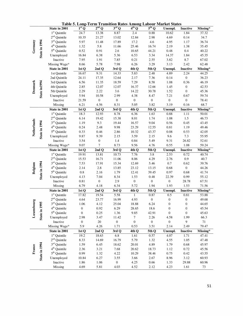
51
Table 5. Long-Term Transition Rates Among Labour Market States
Ger
ma
ny
State in 2001 1st Q 2nd Q 3rd Q 4th Q 5th Q Unempl. Inactive Missing*
Sta
te i
n 1
99
4
1st Quintile 24.7 13.38 8.87 2.4 0.88 10.62 1.84 37.32
2nd Quintile 10.35 21.27 13.02 12.84 2.98 4.69 0.14 34.7
3rd Quintile 5.97 11.48 17.89 17.2 4.6 4.95 1.17 36.74
4th Quintile 1.32 5.8 11.66 25.46 16.74 2.19 1.38 35.45
5th Quintile 0.52 0.91 2.6 10.65 44.21 0.48 0.4 40.22
Unemployed 16.84 6.38 5.36 6.53 3.34 14.37 1.84 45.35
Inactive 7.95 1.91 7.85 0.21 2.55 3.82 8.7 67.02
Missing Wage* 8.66 5.78 7.98 6.26 3.29 3.13 2.42 62.48
Den
mark
State in 2001 1st Q 2nd Q 3rd Q 4th Q 5th Q Unempl. Inactive Missing*
Sta
te i
n19
94
1st Quintile 16.67 9.31 14.33 5.83 2.48 4.89 2.24 44.25
2nd Quintile 24.11 17.35 12.64 2.17 7.36 0.14 0 36.23
3rd Quintile 6.56 11.35 18.59 7.29 8.58 1.08 0.36 46.19
4th Quintile 2.85 12.07 12.07 16.37 12.66 1.45 0 42.53
5th Quintile 2.29 2.22 3.6 14.22 30.78 1.52 0 45.36
Unemployed 5.94 10.58 2.99 4.38 8.47 7.21 0.67 59.74
Inactive 21.59 0 0 0 0 0 0 78.41
Missing 6.21 4.56 8.31 5.05 3.82 3.19 0.16 68.7
Net
her
lna
ds
State in 2001 1st Q 2nd Q 3rd Q 4th Q 5th Q Unempl. Inactive Missing*
Sta
te i
n 1
99
4
1st Quintile 18.3 12.93 8.78 6.36 1.63 0.88 1.11 50.01
2nd Quintile 6.14 19.42 15.38 8.01 1.74 1.08 1.5 46.73
3rd Quintile 1.19 9.3 19.44 16.57 9.04 0.56 0.45 43.45
4th Quintile 0.24 2.48 9.98 23.29 12.55 0.81 1.19 49.46
5th Quintile 0.33 0.46 2.86 10.32 43.37 0.08 0.53 42.05
Unemployed 9.87 9.39 2.15 3.59 2.15 9.6 7.3 55.95
Inactive 3.54 0 1.4 0.84 5.49 9.31 26.82 52.61
Missing Wage* 9.07 7 8.73 9.56 4.76 0.55 1.08 59.24
Bel
giu
m
State in 2001 1st Q 2nd Q 3rd Q 4th Q 5th Q Unempl. Inactive Missing*
Sta
te i
n 1
99
4
1st Quintile 19.91 13.81 10.73 7.76 3.8 2.53 0.72 40.74
2nd Quintile 15.53 16.71 11.06 8.06 4.29 2.76 0.9 40.7
3rd Quintile 7.53 17.91 15.34 12.69 5.46 0.7 0.62 39.76
4th Quintile 2.14 2.8 13.85 23.12 13.15 0.68 0 44.26
5th Quintile 0.8 2.16 1.79 12.41 39.45 0.97 0.68 41.74
Unemployed 4.13 7.04 8.34 1.53 0.48 22.39 0.99 55.12
Inactive 0.81 0 2.9 0 0 0 28.78 67.51
Missing 6.79 4.18 6.34 5.72 1.94 1.93 1.53 71.56
Lu
xem
bo
urg
State in 2001 1st Q 2nd Q 3rd Q 4th Q 5th Q Unempl. Inactive Missing*
Sta
te i
n 1
99
5
1st Quintile 17.82 19.54 5.58 1 0.87 0.5 0.81 53.88
2nd Quintile 4.64 23.77 16.99 4.93 0 0 0 49.68
3rd Quintile 1.06 4.12 25.04 18.88 6.24 0 0 44.65
4th Quintile 0 0.92 6.29 28.65 18.6 0 0 45.54
5th Quintile 0 0.25 1.36 9.85 42.91 0 0 45.63
Unemployed 2.98 3.47 11.42 7 2.26 4.58 1.99 66.3
Inactive 0 20 0 0 0 0 9 71
Missing Wage* 5.9 4.26 1.71 0.53 3.51 2.14 2.49 79.47
Fra
nce
State in 2001 1st Q 2nd Q 3rd Q 4th Q 5th Q Unempl. Inactive Missing*
Sta
te i
n 1
99
4
1st Quintile 19.2 18.63 6.8 1.61 0.57 4.07 1.71 47.41
2nd Quintile 8.33 14.69 16.79 5.79 1.32 4.55 1.05 47.48
3rd Quintile 1.59 6.45 18.62 20.01 4.89 1.79 0.68 45.97
4th Quintile 2.36 3.21 7.68 20.62 18.73 1.12 0.72 45.56
5th Quintile 0.99 1.32 4.22 10.29 38.46 0.75 0.42 43.55
Unemployed 10.84 6.27 3.55 3.66 2.67 8.96 3.12 60.93
Inactive 1.86 1.06 0 4.25 0.66 1.33 29.88 60.96
Missing 4.69 5.81 4.03 4.52 2.12 4.23 1.61 73
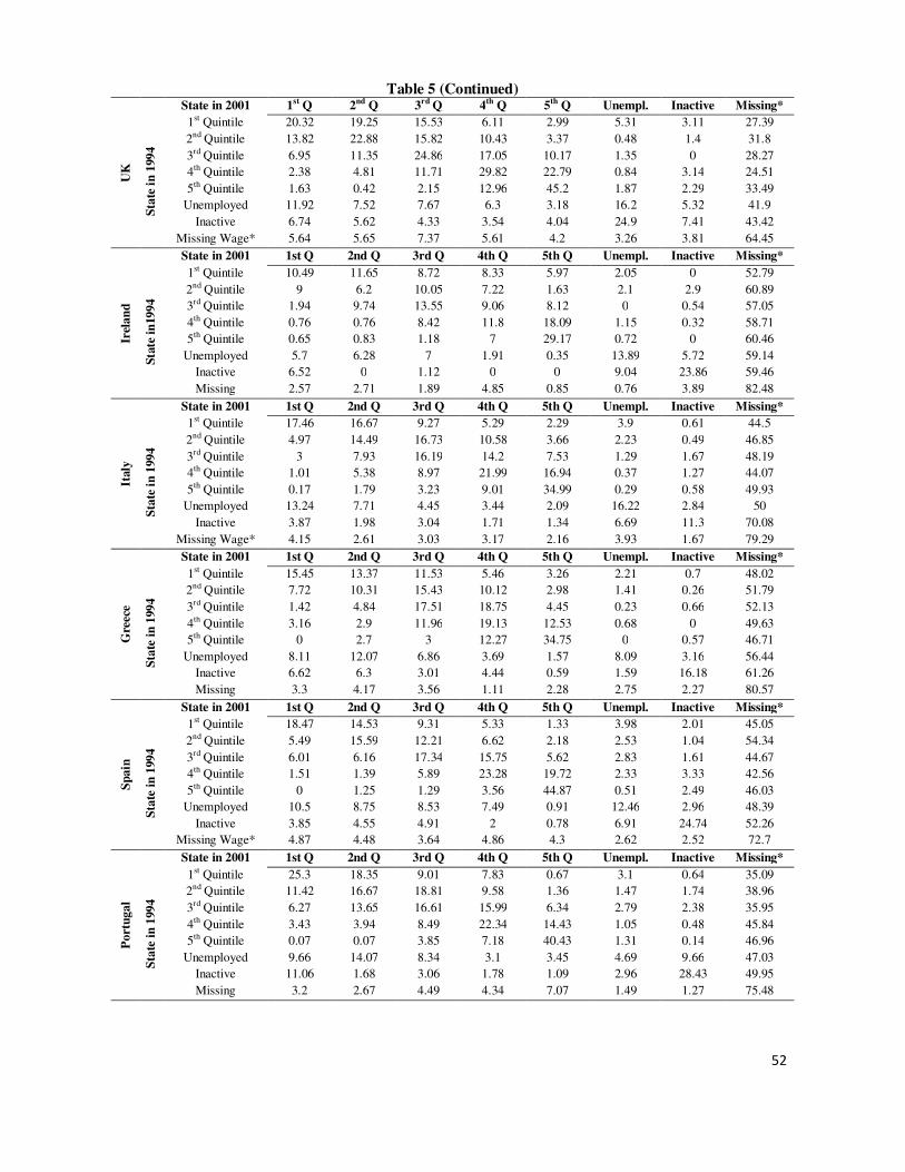
52
Table 5 (Continued)
UK
State in 2001 1st Q 2nd Q 3rd Q 4th Q 5th Q Unempl. Inactive Missing*
Sta
te i
n 1
99
4
1st Quintile 20.32 19.25 15.53 6.11 2.99 5.31 3.11 27.39
2nd Quintile 13.82 22.88 15.82 10.43 3.37 0.48 1.4 31.8
3rd Quintile 6.95 11.35 24.86 17.05 10.17 1.35 0 28.27
4th Quintile 2.38 4.81 11.71 29.82 22.79 0.84 3.14 24.51
5th Quintile 1.63 0.42 2.15 12.96 45.2 1.87 2.29 33.49
Unemployed 11.92 7.52 7.67 6.3 3.18 16.2 5.32 41.9
Inactive 6.74 5.62 4.33 3.54 4.04 24.9 7.41 43.42
Missing Wage* 5.64 5.65 7.37 5.61 4.2 3.26 3.81 64.45
Irel
an
d
State in 2001 1st Q 2nd Q 3rd Q 4th Q 5th Q Unempl. Inactive Missing*
Sta
te i
n19
94
1st Quintile 10.49 11.65 8.72 8.33 5.97 2.05 0 52.79
2nd Quintile 9 6.2 10.05 7.22 1.63 2.1 2.9 60.89
3rd Quintile 1.94 9.74 13.55 9.06 8.12 0 0.54 57.05
4th Quintile 0.76 0.76 8.42 11.8 18.09 1.15 0.32 58.71
5th Quintile 0.65 0.83 1.18 7 29.17 0.72 0 60.46
Unemployed 5.7 6.28 7 1.91 0.35 13.89 5.72 59.14
Inactive 6.52 0 1.12 0 0 9.04 23.86 59.46
Missing 2.57 2.71 1.89 4.85 0.85 0.76 3.89 82.48
Italy
State in 2001 1st Q 2nd Q 3rd Q 4th Q 5th Q Unempl. Inactive Missing*
Sta
te i
n 1
99
4
1st Quintile 17.46 16.67 9.27 5.29 2.29 3.9 0.61 44.5
2nd Quintile 4.97 14.49 16.73 10.58 3.66 2.23 0.49 46.85
3rd Quintile 3 7.93 16.19 14.2 7.53 1.29 1.67 48.19
4th Quintile 1.01 5.38 8.97 21.99 16.94 0.37 1.27 44.07
5th Quintile 0.17 1.79 3.23 9.01 34.99 0.29 0.58 49.93
Unemployed 13.24 7.71 4.45 3.44 2.09 16.22 2.84 50
Inactive 3.87 1.98 3.04 1.71 1.34 6.69 11.3 70.08
Missing Wage* 4.15 2.61 3.03 3.17 2.16 3.93 1.67 79.29
Gre
ece
State in 2001 1st Q 2nd Q 3rd Q 4th Q 5th Q Unempl. Inactive Missing*
Sta
te i
n 1
99
4
1st Quintile 15.45 13.37 11.53 5.46 3.26 2.21 0.7 48.02
2nd Quintile 7.72 10.31 15.43 10.12 2.98 1.41 0.26 51.79
3rd Quintile 1.42 4.84 17.51 18.75 4.45 0.23 0.66 52.13
4th Quintile 3.16 2.9 11.96 19.13 12.53 0.68 0 49.63
5th Quintile 0 2.7 3 12.27 34.75 0 0.57 46.71
Unemployed 8.11 12.07 6.86 3.69 1.57 8.09 3.16 56.44
Inactive 6.62 6.3 3.01 4.44 0.59 1.59 16.18 61.26
Missing 3.3 4.17 3.56 1.11 2.28 2.75 2.27 80.57
Sp
ain
State in 2001 1st Q 2nd Q 3rd Q 4th Q 5th Q Unempl. Inactive Missing*
Sta
te i
n 1
99
4
1st Quintile 18.47 14.53 9.31 5.33 1.33 3.98 2.01 45.05
2nd Quintile 5.49 15.59 12.21 6.62 2.18 2.53 1.04 54.34
3rd Quintile 6.01 6.16 17.34 15.75 5.62 2.83 1.61 44.67
4th Quintile 1.51 1.39 5.89 23.28 19.72 2.33 3.33 42.56
5th Quintile 0 1.25 1.29 3.56 44.87 0.51 2.49 46.03
Unemployed 10.5 8.75 8.53 7.49 0.91 12.46 2.96 48.39
Inactive 3.85 4.55 4.91 2 0.78 6.91 24.74 52.26
Missing Wage* 4.87 4.48 3.64 4.86 4.3 2.62 2.52 72.7
Po
rtu
ga
l
State in 2001 1st Q 2nd Q 3rd Q 4th Q 5th Q Unempl. Inactive Missing*
Sta
te i
n 1
99
4
1st Quintile 25.3 18.35 9.01 7.83 0.67 3.1 0.64 35.09
2nd Quintile 11.42 16.67 18.81 9.58 1.36 1.47 1.74 38.96
3rd Quintile 6.27 13.65 16.61 15.99 6.34 2.79 2.38 35.95
4th Quintile 3.43 3.94 8.49 22.34 14.43 1.05 0.48 45.84
5th Quintile 0.07 0.07 3.85 7.18 40.43 1.31 0.14 46.96
Unemployed 9.66 14.07 8.34 3.1 3.45 4.69 9.66 47.03
Inactive 11.06 1.68 3.06 1.78 1.09 2.96 28.43 49.95
Missing 3.2 2.67 4.49 4.34 7.07 1.49 1.27 75.48

53
Table 5 (Continued)
Au
stri
a
State in 2001 1st Q 2nd Q 3rd Q 4th Q 5th Q Unempl. Inactive Missing*
Sta
te i
n 1
99
5
1st Quintile 23.54 16.86 7.6 3.13 1.94 2.25 0.39 44.3
2nd Quintile 10.63 14.49 17.77 11.53 2.8 3.11 0 39.68
3rd Quintile 8.85 12.93 11.45 14.4 5.82 4.3 0.41 41.84
4th Quintile 0.62 5.86 7.46 24.87 13.32 1.24 0.59 46.04
5th Quintile 1.51 3.15 3.85 8.84 35.19 1.14 0 46.32
Unemployed 10.27 1.15 3.58 1.73 2.08 19.03 0 62.17
Inactive 14.29 0 2.81 6.63 2.3 0.51 9.18 64.29
Missing Wage* 4.91 3.65 3.63 1.3 3.4 0.17 0.14 82.81
Fin
lan
d
State in 2001 1st Q 2nd Q 3rd Q 4th Q 5th Q Unempl. Inactive Missing*
Sta
te i
n19
96
1st Quintile 20.59 11.87 7.01 6.76 2.68 2.12 0.6 48.37
2nd Quintile 7.29 19.15 19.27 10.53 1.95 0.56 0.28 40.98
3rd Quintile 5.07 10.82 21.71 14.7 8.04 2 0 37.66
4th Quintile 0.69 4.32 10.95 20.96 17.83 1.64 0 43.59
5th Quintile 1.72 0.95 3.88 10.79 35.23 0.67 0.29 46.47
Unemployed 14.51 9.58 5.16 3.49 1.45 12.88 0.83 52.1
Inactive 0 0 4.57 2.74 0 6.39 0 86.3
Missing 5.66 4.51 4.35 5.08 4.25 3.17 1.81 71.16
* Missing Wage refers to individuals with missing wage in the first wave and Missing refers to individuals with missing wage, self-
employed, retired, not in formal employment and those that dropped from the survey in the previous year.

54
Table 6. Short-Term Transition Rates Among Income Quintiles
Ger
man
y
State in 1995
State in 1994 1st Quintile 2nd Quintile 3rd Quintile 4th Quintile 5th Quintile
1st Quintile 71.28 21.63 6 1.09 0
2nd Quintile 15.93 55.46 20.42 7.22 0.98
3rd Quintile 4.15 19.68 49.2 23.36 3.62
4th Quintile 0.47 4.82 20.38 55.66 18.67
5th Quintile 0 0.5 2.56 12.9 84.03
State in 2001
State in 2000 1st Quintile 2nd Quintile 3rd Quintile 4th Quintile 5th Quintile
1st Quintile 77.43 17.39 4.21 0.74 0.23
2nd Quintile 17.75 57.19 20.3 4.34 0.41
3rd Quintile 3.68 21.97 53.15 20.09 1.12
4th Quintile 0.6 2.63 15.79 66.86 14.13
5th Quintile 0.58 2.55 2.91 14.89 79.08
Den
mark
State in 1995
State in 1994 1st Quintile 2nd Quintile 3rd Quintile 4th Quintile 5th Quintile
1st Quintile 55.54 26.12 13.4 2.28 2.67
2nd Quintile 25.15 47.93 17.03 8.63 1.26
3rd Quintile 7.03 34.02 32.22 19.84 6.89
4th Quintile 0.88 7.75 25.73 48.91 16.73
5th Quintile 2.42 1.15 1.82 27.9 66.71
State in 2001
State in 2000 1st Quintile 2nd Quintile 3rd Quintile 4th Quintile 5th Quintile
1st Quintile 60.81 20.21 15.94 2.17 0.87
2nd Quintile 28.36 41.29 21.36 3.45 5.54
3rd Quintile 6.61 23.05 50.56 16.36 3.42
4th Quintile 4.81 9.09 23.02 43.4 19.68
5th Quintile 0.66 0.77 6.44 15.01 77.12
Net
her
lan
ds
State in 1995
State in 1994 1st Quintile 2nd Quintile 3rd Quintile 4th Quintile 5th Quintile
1st Quintile 61.88 29.72 6.16 2.14 0.09
2nd Quintile 13.02 51.22 27.54 6.55 1.66
3rd Quintile 3.33 16.08 51.68 25.46 3.45
4th Quintile 0.58 3.04 14.91 59.91 21.56
5th Quintile 1 0.55 2.58 14.92 80.94
State in 2001
State in 2000 1st Quintile 2nd Quintile 3rd Quintile 4th Quintile 5th Quintile
1st Quintile 71.13 20.01 4.7 3.56 0.6
2nd Quintile 9.31 59.25 22.57 7.3 1.56
3rd Quintile 5.55 8.59 61.68 19 5.18
4th Quintile 1.04 1.41 18.41 63.84 15.3
5th Quintile 0 0.85 1.43 18.22 79.5
Bel
giu
m
State in 1995
State in 1994 1st Quintile 2nd Quintile 3rd Quintile 4th Quintile 5th Quintile
1st Quintile 54.42 20.13 12.22 8.2 5.03
2nd Quintile 28.54 43.39 18.78 7.72 1.57
3rd Quintile 5.96 28.14 48.55 12.84 4.51
4th Quintile 3.7 5.64 24.09 49.88 16.68
5th Quintile 0.71 1.68 3.09 18.49 76.02
State in 2001
State in 2000 1st Quintile 2nd Quintile 3rd Quintile 4th Quintile 5th Quintile
1st Quintile 72.75 17.92 8.59 0.39 0.35
2nd Quintile 12.7 54.52 23.99 6.7 2.09
3rd Quintile 6.37 20.15 43.23 27.42 2.82
4th Quintile 0.98 6.51 22.88 54.85 14.79
5th Quintile 0 1.44 1.78 18.18 78.6

55
Lu
xem
bo
urg
State in 1996
State in 1995 1st Quintile 2nd Quintile 3rd Quintile 4th Quintile 5th Quintile
1st Quintile 76.59 20.03 1.42 0.88 1.09
2nd Quintile 15.78 66.6 17.11 0.23 0.27
3rd Quintile 2.82 14.51 68.15 10.46 4.05
4th Quintile 0.25 0.7 21.98 64.35 12.73
5th Quintile 0.3 0 4.12 16.95 78.62
State in 2001
State in 2000 1st Quintile 2nd Quintile 3rd Quintile 4th Quintile 5th Quintile
1st Quintile 70.77 26.87 1.75 0.61 0
2nd Quintile 11.44 67.15 19.03 1.74 0.64
3rd Quintile 2.87 6.29 68.93 21.06 0.85
4th Quintile 0.3 1.36 10.26 69.22 18.86
5th Quintile 0 0.23 0.33 12.24 87.2
Fra
nce
State in 1995
State in 1994 1st Quintile 2nd Quintile 3rd Quintile 4th Quintile 5th Quintile
1st Quintile 65.42 25.5 7.18 1.2 0.71
2nd Quintile 15.11 55.45 24.6 3.91 0.93
3rd Quintile 4.84 17.24 51.07 23.84 3.02
4th Quintile 2.59 5.09 15.85 54.3 22.18
5th Quintile 3.17 2.67 4.29 16.67 73.2
State in 2001
State in 2000 1st Quintile 2nd Quintile 3rd Quintile 4th Quintile 5th Quintile
1st Quintile 66.52 22.09 7.91 2.74 0.75
2nd Quintile 20.07 55.68 20.16 3.74 0.35
3rd Quintile 2.57 17.98 59.08 19.28 1.09
4th Quintile 0.67 3.7 14.23 64.29 17.1
5th Quintile 0.51 0.21 1.8 13 84.47
UK
State in 1995
State in 1994 1st Quintile 2nd Quintile 3rd Quintile 4th Quintile 5th Quintile
1st Quintile 58.66 28.75 6.7 4.14 1.75
2nd Quintile 24.05 49.87 19.05 4.93 2.1
3rd Quintile 4.58 15.68 54.34 22.38 3.01
4th Quintile 0.13 4.4 19.78 59.68 16.01
5th Quintile 0.94 0.74 3.04 13.82 81.46
State in 2001
State in 2000 1st Quintile 2nd Quintile 3rd Quintile 4th Quintile 5th Quintile
1st Quintile 59.09 29.59 7 2.17 2.15
2nd Quintile 23 46.06 22.44 6.43 2.08
3rd Quintile 4.37 19.4 53.07 20.07 3.08
4th Quintile 0.92 3.76 17.91 60.66 16.75
5th Quintile 0.64 2.08 3.04 15.79 78.44
Irel
an
d
State in 1995
State in 1994 1st Quintile 2nd Quintile 3rd Quintile 4th Quintile 5th Quintile
1st Quintile 61.64 23.6 7.93 5.45 1.37
2nd Quintile 18.52 51.61 20.32 7.21 2.34
3rd Quintile 2.2 21.77 48.92 26.09 1.01
4th Quintile 0.89 4.06 24.16 48.96 21.92
5th Quintile 0 0.45 4.75 14.63 80.17
State in 2001
State in 2000 1st Quintile 2nd Quintile 3rd Quintile 4th Quintile 5th Quintile
1st Quintile 64.62 21.88 9.76 3.73 0
2nd Quintile 20.41 50.8 18.82 7.71 2.26
3rd Quintile 4.54 24.16 49.53 17.58 4.19
4th Quintile 1.27 5.22 20.3 51.82 21.4
5th Quintile 0 3.42 3.53 19.1 73.96

56
Italy
State in 1995
State in 1994 1st Quintile 2nd Quintile 3rd Quintile 4th Quintile 5th Quintile
1st Quintile 68.84 18.2 8.05 4.24 0.67
2nd Quintile 17.92 42.29 26.35 10.29 3.15
3rd Quintile 5.66 17.79 47.58 23.95 5.02
4th Quintile 3.19 8.88 15.85 51.05 21.03
5th Quintile 1.96 1.71 3.2 18.64 74.49
State in 2001
State in 2000 1st Quintile 2nd Quintile 3rd Quintile 4th Quintile 5th Quintile
1st Quintile 69.26 18.82 5.83 3.76 2.33
2nd Quintile 14.83 54.54 24.01 4.8 1.82
3rd Quintile 2.49 21.25 52.9 19.4 3.96
4th Quintile 1.31 4.49 20.02 58.22 15.96
5th Quintile 0.44 2.32 2.39 15.13 79.72
Gre
ece
State in 1995
State in 1994 1st Quintile 2nd Quintile 3rd Quintile 4th Quintile 5th Quintile
1st Quintile 54.34 27.71 12.62 2.85 2.5
2nd Quintile 20.63 35.96 32.26 6.08 5.06
3rd Quintile 5.79 20.71 42.39 23.9 7.21
4th Quintile 3.52 7.7 24.04 43.16 21.59
5th Quintile 0.81 3.63 8.96 20.96 65.64
State in 2001
State in 2000 1st Quintile 2nd Quintile 3rd Quintile 4th Quintile 5th Quintile
1st Quintile 69.46 23.48 5.31 1.3 0.45
2nd Quintile 11.78 57.39 22.8 7.14 0.89
3rd Quintile 4.7 15.7 61.55 15.34 2.7
4th Quintile 0 2.38 19.38 57.24 21
5th Quintile 0 0.56 2.85 11.94 84.65
Sp
ain
State in 1995
State in 1994 1st Quintile 2nd Quintile 3rd Quintile 4th Quintile 5th Quintile
1st Quintile 54.57 30.02 12.97 2.2 0.25
2nd Quintile 18.99 42.66 29.77 7.53 1.04
3rd Quintile 6.21 17.02 44.84 28.03 3.91
4th Quintile 0.43 3.11 13.34 58.36 24.75
5th Quintile 0.47 0.29 1.43 17.12 80.7
State in 2001
State in 2000 1st Quintile 2nd Quintile 3rd Quintile 4th Quintile 5th Quintile
1st Quintile 49.63 30.21 11.28 8.39 0.49
2nd Quintile 25.07 40.72 21.78 12.09 0.33
3rd Quintile 9.25 20.89 47.33 18.07 4.46
4th Quintile 4.18 5.96 21.67 48.66 19.53
5th Quintile 0 1.48 1.28 17.65 79.59
Po
rtu
ga
l
State in 1995
State in 1994 1st Quintile 2nd Quintile 3rd Quintile 4th Quintile 5th Quintile
1st Quintile 59.43 27.21 10.27 2.9 0.2
2nd Quintile 19.05 50.16 25.92 4.88 0
3rd Quintile 6.08 14.46 54.58 22.67 2.22
4th Quintile 2.36 7.44 15.25 63.39 11.56
5th Quintile 0.04 0.25 2.08 10.65 86.98
State in 2001
State in 2000 1st Quintile 2nd Quintile 3rd Quintile 4th Quintile 5th Quintile
1st Quintile 78.36 12.12 4.91 2.64 1.96
2nd Quintile 15.2 56.42 24.64 3.64 0.11
3rd Quintile 5.45 11.07 59.26 16.97 7.25
4th Quintile 0.08 6.86 19.58 65.75 7.73
5th Quintile 0 0.54 2.73 11.48 85.25

57
Au
stri
a
State in 1995
State in 1994 1st Quintile 2nd Quintile 3rd Quintile 4th Quintile 5th Quintile
1st Quintile 59.34 29.58 6.42 2.93 1.73
2nd Quintile 22.45 39.77 25.53 9.03 3.21
3rd Quintile 12.81 29.32 27.53 24.62 5.72
4th Quintile 4.69 6.97 22.91 41.81 23.62
5th Quintile 0.78 4.17 3.99 21.47 69.59
State in 2001
State in 2000 1st Quintile 2nd Quintile 3rd Quintile 4th Quintile 5th Quintile
1st Quintile 76.91 14.99 5.19 2.2 0.72
2nd Quintile 15.42 58.33 17.17 6.42 2.66
3rd Quintile 8.74 18.23 54.11 15.35 3.57
4th Quintile 2.48 2.98 12.26 64.18 18.1
5th Quintile 0 1.25 1.99 16.55 80.21
Fin
lan
d*
State in 1997
State in 1996 1st Quintile 2nd Quintile 3rd Quintile 4th Quintile 5th Quintile
1st Quintile 61.68 24.64 7.23 4.79 1.67
2nd Quintile 12.84 52.25 25.39 5.87 3.65
3rd Quintile 6.06 24.29 43.99 18.55 7.1
4th Quintile 1.88 6.31 23.27 51.2 17.34
5th Quintile 1.03 2.06 7.08 18.4 71.42
State in 2001
State in 2000 1st Quintile 2nd Quintile 3rd Quintile 4th Quintile 5th Quintile
1st Quintile 57.17 27.26 11.38 2.4 1.79
2nd Quintile 23.31 40.69 25.82 6.31 3.88
3rd Quintile 2.56 21.84 47.24 26.16 2.21
4th Quintile 3.59 4.35 16.45 54.82 20.8
5th Quintile 1.01 1.05 5.45 18.9 73.6
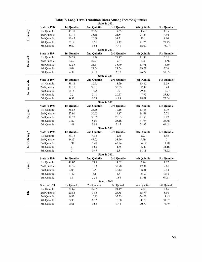
58
Table 7. Long-Term Transition Rates Among Income Quintiles
Ger
ma
ny
State in 2001
State in 1994 1st Quintile 2nd Quintile 3rd Quintile 4th Quintile 5th Quintile
1st Quintile 49.18 26.64 17.65 4.77 1.75
2nd Quintile 17.11 35.18 21.54 21.24 4.92
3rd Quintile 10.45 20.09 31.31 30.1 8.06
4th Quintile 2.17 9.51 19.12 41.76 27.45
5th Quintile 0.89 1.54 4.41 18.09 75.07
Den
mark
State in 2001
State in 1994 1st Quintile 2nd Quintile 3rd Quintile 4th Quintile 5th Quintile
1st Quintile 34.28 19.16 29.47 11.98 5.11
2nd Quintile 37.9 27.27 19.87 3.4 11.56
3rd Quintile 12.53 21.67 35.49 13.91 16.39
4th Quintile 5.09 21.54 21.54 29.22 22.6
5th Quintile 4.32 4.18 6.77 26.77 57.95
Net
her
lan
ds
State in 2001
State in 1994 1st Quintile 2nd Quintile 3rd Quintile 4th Quintile 5th Quintile
1st Quintile 38.12 26.95 18.29 13.26 3.39
2nd Quintile 12.11 38.31 30.35 15.8 3.43
3rd Quintile 2.14 16.75 35 29.83 16.27
4th Quintile 0.5 5.11 20.57 47.97 25.85
5th Quintile 0.57 0.79 4.99 18.01 75.64
Bel
giu
m
State in 2001
State in 1994 1st Quintile 2nd Quintile 3rd Quintile 4th Quintile 5th Quintile
1st Quintile 35.55 24.66 19.16 13.85 6.79
2nd Quintile 27.91 30.03 19.87 14.48 7.71
3rd Quintile 12.77 30.39 26.03 21.53 9.27
4th Quintile 3.89 5.09 25.16 41.98 23.88
5th Quintile 1.41 3.82 3.17 21.92 69.68
Lu
xem
bo
urg
*
State in 2001
State in 1995 1st Quintile 2nd Quintile 3rd Quintile 4th Quintile 5th Quintile
1st Quintile 39.78 43.6 12.45 2.23 1.95
2nd Quintile 9.22 47.23 33.76 9.79 0
3rd Quintile 1.92 7.45 45.24 34.12 11.28
4th Quintile 0 1.69 11.55 52.6 34.16
5th Quintile 0 0.47 2.5 18.11 78.92
Fra
nce
State in 2001
State in 1994 1st Quintile 2nd Quintile 3rd Quintile 4th Quintile 5th Quintile
1st Quintile 41.02 39.8 14.52 3.44 1.22
2nd Quintile 17.76 31.3 35.78 12.34 2.81
3rd Quintile 3.08 12.51 36.12 38.81 9.48
4th Quintile 4.49 6.1 14.61 39.2 35.6
5th Quintile 1.8 2.38 7.64 18.61 69.57
UK
State in 2001
State in 1994 1st Quintile 2nd Quintile 3rd Quintile 4th Quintile 5th Quintile
1st Quintile 31.65 29.99 24.19 9.52 4.65
2nd Quintile 20.84 34.5 23.85 15.73 5.08
3rd Quintile 9.87 16.13 35.33 24.23 14.45
4th Quintile 3.33 6.72 16.38 41.7 31.87
5th Quintile 2.61 0.68 3.44 20.79 72.49
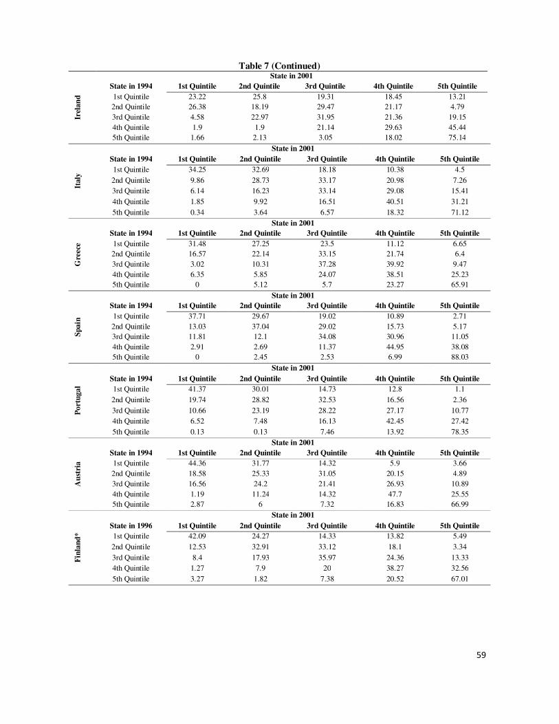
59
Table 7 (Continued)
Irel
an
d
State in 2001
State in 1994 1st Quintile 2nd Quintile 3rd Quintile 4th Quintile 5th Quintile
1st Quintile 23.22 25.8 19.31 18.45 13.21
2nd Quintile 26.38 18.19 29.47 21.17 4.79
3rd Quintile 4.58 22.97 31.95 21.36 19.15
4th Quintile 1.9 1.9 21.14 29.63 45.44
5th Quintile 1.66 2.13 3.05 18.02 75.14
Italy
State in 2001
State in 1994 1st Quintile 2nd Quintile 3rd Quintile 4th Quintile 5th Quintile
1st Quintile 34.25 32.69 18.18 10.38 4.5
2nd Quintile 9.86 28.73 33.17 20.98 7.26
3rd Quintile 6.14 16.23 33.14 29.08 15.41
4th Quintile 1.85 9.92 16.51 40.51 31.21
5th Quintile 0.34 3.64 6.57 18.32 71.12
Gre
ece
State in 2001
State in 1994 1st Quintile 2nd Quintile 3rd Quintile 4th Quintile 5th Quintile
1st Quintile 31.48 27.25 23.5 11.12 6.65
2nd Quintile 16.57 22.14 33.15 21.74 6.4
3rd Quintile 3.02 10.31 37.28 39.92 9.47
4th Quintile 6.35 5.85 24.07 38.51 25.23
5th Quintile 0 5.12 5.7 23.27 65.91
Sp
ain
State in 2001
State in 1994 1st Quintile 2nd Quintile 3rd Quintile 4th Quintile 5th Quintile
1st Quintile 37.71 29.67 19.02 10.89 2.71
2nd Quintile 13.03 37.04 29.02 15.73 5.17
3rd Quintile 11.81 12.1 34.08 30.96 11.05
4th Quintile 2.91 2.69 11.37 44.95 38.08
5th Quintile 0 2.45 2.53 6.99 88.03
Po
rtu
ga
l
State in 2001
State in 1994 1st Quintile 2nd Quintile 3rd Quintile 4th Quintile 5th Quintile
1st Quintile 41.37 30.01 14.73 12.8 1.1
2nd Quintile 19.74 28.82 32.53 16.56 2.36
3rd Quintile 10.66 23.19 28.22 27.17 10.77
4th Quintile 6.52 7.48 16.13 42.45 27.42
5th Quintile 0.13 0.13 7.46 13.92 78.35
Au
stri
a
State in 2001
State in 1994 1st Quintile 2nd Quintile 3rd Quintile 4th Quintile 5th Quintile
1st Quintile 44.36 31.77 14.32 5.9 3.66
2nd Quintile 18.58 25.33 31.05 20.15 4.89
3rd Quintile 16.56 24.2 21.41 26.93 10.89
4th Quintile 1.19 11.24 14.32 47.7 25.55
5th Quintile 2.87 6 7.32 16.83 66.99
Fin
lan
d*
State in 2001
State in 1996 1st Quintile 2nd Quintile 3rd Quintile 4th Quintile 5th Quintile
1st Quintile 42.09 24.27 14.33 13.82 5.49
2nd Quintile 12.53 32.91 33.12 18.1 3.34
3rd Quintile 8.4 17.93 35.97 24.36 13.33
4th Quintile 1.27 7.9 20 38.27 32.56
5th Quintile 3.27 1.82 7.38 20.52 67.01

60
Table 8 Immobility Ratio (IR) and Average Jump (AJ) for 1-year and 7-year Transition Rates of
Earnings Quintiles (%)
Country Period IR IR/
IR(perfect mobility) AJ
AJ/
AJ(perfect mobility)
Germany 1-year
1994-1995 0.937 1.802 0.438 0.274
2000-2001 0.952 1.831 0.392 0.245
8-year 1994-2001 0.825 1.587 0.747 0.467
Denmark 1-year
1994-1995 0.888 1.707 0.641 0.401
2000-2001 0.880 1.693 0.606 0.379
8-year 1994-2001 0.735 1.414 1.000 0.625
Netherlands 1-year
1994-1995 0.938 1.803 0.465 0.291
2000-2001 0.934 1.795 0.412 0.257
8-year 1994-2001 0.831 1.598 0.751 0.469
Belgium 1-year
1994-1995 0.880 1.692 0.629 0.393
2000-2001 0.924 1.777 0.403 0.252
8-year 1994-2001 0.797 1.533 0.888 0.555
Luxembourg* 1-year
1995-1996 0.968 1.861 0.332 0.207
2000-2001 0.979 1.882 0.298 0.186
8-year 1995-2001 0.911 1.753 0.574 0.359
France 1-year
1994-1995 0.921 1.771 0.511 0.319
2000-2001 0.948 1.823 0.405 0.253
8-year 1994-2001 0.861 1.657 0.742 0.464
UK 1-year
1994-1995 0.927 1.783 0.490 0.306
2000-2001 0.925 1.778 0.506 0.317
8-year 1994-2001 0.800 1.538 0.836 0.522
Ireland 1-year
1994-1995 0.925 1.778 0.516 0.323
2000-2001 0.909 1.748 0.531 0.332
8-year 1994-2001 0.777 1.495 0.980 0.613
Italy 1-year
1994-1995 0.888 1.708 0.579 0.362
2000-2001 0.928 1.785 0.472 0.295
8-year 1994-2001 0.790 1.519 0.860 0.538
Greece 1-year
1994-1995 0.867 1.667 0.694 0.434
2000-2001 0.943 1.814 0.403 0.252
8-year 1994-2001 0.790 1.520 0.904 0.565
Spain 1-year
1994-1995 0.920 1.770 0.528 0.330
2000-2001 0.882 1.695 0.617 0.386
8-year 1994-2001 0.826 1.589 0.744 0.465
Portugal 1-year
1994-1995 0.923 1.774 0.460 0.288
2000-2001 0.928 1.784 0.397 0.248
8-year 1994-2001 0.819 1.574 0.792 0.495
Austria 1-year
1995-1996 0.875 1.683 0.689 0.431
2000-2001 0.924 1.776 0.429 0.268
7-year 1995-2001 0.790 1.519 0.861 0.538
Finland 1-year
1996-1997 0.891 1.713 0.584 0.365
2000-2001 0.908 1.746 0.578 0.361
6-year 1996-2001 0.803 1.544 0.840 0.525

61
Table 9. Mobility Index for different time horizons over time: Year 1994-2001 (Index*100)
Time Horizon Mobility Index
G Dk Nl Be Lu Fr UK Ir It Gr Sp Pt Au Fi
1994-1995 18.85 26.65 19.33 27.01
22.50 21.12 21.43 25.52 29.52 21.51 20.64
1994-1996 22.25 31.44 20.16 28.22
24.34 23.87 27.59 27.92 30.24 24.89 25.57
1994-1997 24.19 35.45 22.64 31.08
25.88 26.04 29.88 30.40 31.51 24.96 27.28
1994-1998 25.12 38.86 25.88 29.97
25.09 29.19 33.11 32.91 33.18 25.67 28.32
1994-1999 26.48 38.50 27.55 33.30
27.92 30.48 33.46 33.26 32.39 27.45 30.32
1994-2000 28.11 40.51 30.47 35.07
29.12 33.83 35.55 34.27 35.86 30.33 32.26
1994-2001 30.54 42.69 31.77 37.20
29.95 35.10 38.36 35.39 37.81 29.60 31.97
1995-1996 20.15 26.72 17.54 22.53 14.39 18.51 20.35 21.99 23.42 22.52 22.16 17.96 28.61
1995-1997 22.82 30.28 21.48 26.17 17.04 20.60 23.30 25.11 27.30 28.16 22.67 21.68 31.17
1995-1998 24.30 33.18 25.34 25.56 17.20 19.66 26.74 27.43 30.02 31.79 24.31 23.82 32.13
1995-1999 25.55 34.69 27.30 28.53 18.82 22.30 29.23 30.06 30.57 32.90 25.28 27.10 34.68
1995-2000 27.80 37.04 31.45 31.41 20.46 24.55 31.26 33.41 32.20 32.37 27.17 29.30 36.01
1995-2001 28.69 39.72 31.92 33.20 22.42 25.00 31.79 36.47 33.69 33.12 27.23 30.44 35.65
1996-1997 19.67 26.43 18.43 23.82 14.65 18.06 20.65 20.25 24.31 23.81 21.54 18.09 21.80 26.39
1996-1998 21.50 33.17 22.37 24.26 15.75 18.38 24.74 24.19 27.80 30.97 24.21 21.96 24.91 30.39
1996-1999 23.77 36.41 26.33 26.93 17.43 20.73 27.68 27.18 29.81 30.26 25.46 25.43 28.53 34.59
1996-2000 27.08 40.07 29.61 29.79 18.91 22.76 30.25 32.42 30.21 31.27 28.58 27.05 30.03 35.78
1996-2001 28.30 39.86 31.16 30.68 20.11 22.83 32.29 32.22 32.63 30.93 28.57 30.13 32.77 36.54
1997-1998 18.76 29.22 20.50 22.13 13.70 15.70 20.63 22.10 23.38 24.15 21.23 16.47 20.97 25.79
1997-1999 21.45 29.81 24.22 26.07 16.46 18.82 24.50 25.83 26.17 25.85 23.94 22.26 25.19 29.70
1997-2000 23.56 32.87 27.86 26.64 18.47 21.48 26.84 29.89 27.90 26.66 27.15 25.47 28.20 32.23
1997-2001 26.36 35.09 30.39 29.98 20.17 22.30 28.88 30.98 30.85 27.87 28.60 28.62 29.74 34.53
1998-1999 16.91 25.97 19.75 23.88 11.30 16.16 21.73 22.33 21.82 20.49 21.91 15.35 19.56 26.02
1998-2000 20.72 32.51 24.17 25.45 13.75 19.82 24.97 27.86 24.49 23.98 23.38 24.12 24.56 31.11
1998-2001 22.86 33.33 25.81 27.63 16.04 20.05 27.85 28.90 27.39 25.34 26.40 26.77 26.33 32.48
1999-2000 17.82 28.55 21.46 23.17 13.38 17.26 21.51 24.99 21.25 16.56 23.69 18.26 20.54 25.89
1999-2001 20.69 28.77 24.38 25.62 14.51 18.36 25.07 29.14 24.71 21.11 26.45 22.27 23.99 28.21
2000-2001 17.44 27.08 19.00 20.71 13.07 17.28 21.67 23.37 20.53 18.68 26.08 17.17 19.16 25.27

62
BIBLIOGRAPHY
Aaberge, Rolf, Bjorklund, Anders, Jantti, Markus, Palme, Marten, Pedersen, Peder J., Smith,
Nina, and Wannemo, Tom. 2002. Income inequlaity and income mobility in the Scandinavian countries compared to the United States. Review of Income and Wealth,
48(4). Atkinson, Anthony, B., Bourguignon, Francois, and Morrisson, C. (Eds.). (1992). Empirical
studies of earnings mobility: Suisse : Harwood Academic Publishers. Brukhauser, Richard V., Holtz-Eakin, Douglas, and Rhody, Stephen E. 1998. Mobility and
inequality in the 1980s: a cross-national comparison of the Unite States and Germany. In Jenkins, Kapteyn andVan Praag (Eds.), The distribution of welfare and household
production (pp. 111-175). Cambridge: Cambridge University Press.
Brukhauser, Richard V., and Poupore, John G. 1997. A cross-national comparison of
permanent inequality in the United States and Germany. Review of Economics and
Statistics, 79, 10-17.
Creedy, J., and Wilhelm, M. 2002. Income Mobility, Inequality and Social Welfare.
Australian Economic Papers, 41(2), 140-150.
Dickens, Richard. 1999. Caught in a trap? Wage mobility in Great Britain: 1975-1994.
Economica(67), 477-497. Duncan, Greg J., and Morgan, James N. 1981. Persistence an change in economic status and
the role of changing family composition. In Hill, Hill andMorgan (Eds.), Five
thousand American families: patterns of economic progress (Vol. 9, pp. 1-44). Ann
Arbor: Institute for Social Resarch, University of Michigan.
Fields, Gary S., Leary, Jesse, and Ok, Efe. 2003. Stochastic dominance in mobility analysis.
Economic Letters, 75(3), 333-339.
Fields, Gary S., and Ok, Efe. 1999. The measurement of income mobility: an introduction to
the literature. In Silber (Ed.), Handbook of Income Inequality Measurement. Boston:
Kluwer Academic Publishing.
Friedman, M. 1962. Capitalism and Freedom. Chicago: University of Chicago Press.
Fritzell, Johan. 1990. The dynamics of income distributions: economic mobility in Sweden in
comparizon with the United States. Social Science Research, 17-46.
Gottschalk, Peter, and Spolaore, Enrico. 2002. On the evaluation of economic mobility.
Review of Economic Studies, 68, 191-208. OECD. 1996. Earnings inequality, low paid employment and earnings mobility. In
Employment Outlook (pp. 59-99). Paris: OECD. OECD. 1997. Earnings mobility: taking a longer view. In Employment Outlook. Paris:
OECD. OECD. 2004. Employment Outlook. Paris: OECD.
OECD. 2006. Labour Market Performance since 1994 and Future Challenges. In Employment
Outlook.
Top Related