


Languages
Pages
Legal

Improved Power System Stabilizer by Applying LQG Controller
ALI M. YOUSEF1, MOHAMED ZAHRAN
2 & GHAREEB MOUSTAFA
3
1. Electrical Eng. Dept. Faculty of Engineering, Assiut University, 71516 Egypt, 2. Electronics Research Institute, Photovoltaic Cells Departments, NRC Blg., El-Tahrir St.,
Dokki, 12311-Giza, Egypt, 3. Electrical Eng. Dept. Faculty of Engineering, Suez Canal University, Ismailia, Egypt,
[email protected], [email protected], [email protected]
Abstract: Power system stabilizers (PSSs) are traditionally used to provide damping torque for the synchronous
generators to suppress the oscillations by generating supplementary control signals for the generator excitation
system. Numerous techniques have previously been proposed to design PSSs but many of them are synthesized
based on a linearized model. The dynamic characteristics of the proposed PSS are studied in a typical
synchronous machine connected to infinite-bus of power system through transmission line. This paper deals
with the applying of the Linear Quadratic Gaussian (LQG) technique to the design of the robust controller for
two models of power system. The first model represents only the electrical control part of power system by
means synchronous generator connected to infinite bus, while the second model, adding a turbine and governor
to the model 1. Combined the Kalman filter, which is an optimal observer with the optimal LQR regulator to
construct the optimal LQG controller are evaluated. Electromechanical oscillations of small magnitude and low
frequency exist in the power system operation and often persist for long periods of time. Simulation results
show the proposed PSS is robust for such nonlinear dynamic system and achieves better performance than the
conventional PSS in damping oscillations.
Key Words: Power System Stabilization, Advanced Controller, Robust Systems Control, LQR, LQG
1. Introduction The power flow at and around the nominal power frequency, all electrical and electromechanical power systems involve a wide range of resonant oscillatory modes. Due to the proximity of generation to the load, small variations in the system load can excite the voltage oscillation due to reactive power mismatch which must be damped to maintain secure and stable system operation. Conventional excitation controllers coupled with power system stabilizers (PSSs) for centralized generation are usually designed based on linearized models. As the load over the entire transmission gets averaged out, linearized generator models are appropriate for designing the oscillation damping controller. But in power distribution systems (PDSs), the load change in proportion to the generation is large and linearized generator models are constantly changing. In such situations, robust control is essential [1]. Damping inter-area oscillations is one of the major concerns for the electric power system operators. With ever increasing power exchange between utilities over the existing transmission network, the problem has become even more challenging. Secure operation of power systems, thus, requires the application of robust controllers to damp these inter-area oscillations. Power system stabilizers (PSSs) are the most commonly used devices for this purpose. The task of control design is challenging, owing to the
complex nature of the interactions in the inter-area modes of the system. Methods received increased attention in power systems; however, issues with weighting function selection make the whole design procedure difficult. Linear quadratic Gaussian (LQG) control approaches using different FACTS devices have been presented for closed-loop identification in, and power system stabilizer (PSS) for small systems in [2]. The basic objective of the control system is the ability to measure the output of the system, and to take corrective action if its value deviates from some desired value. The voltage regulator is the intelligence of the system and controls the output of the exciter so that the generated voltage and reactive power change in the desired way. As the number of power plants with automatic voltage regulators grew, it became apparent that the high performance of these voltage regulators had a destabilizing effect on the power system. Power oscillations of small magnitude and low frequency often persisted for long periods of time. In some cases, this presented a limitation on the amount of power able to be transmitted within the system. Power system stabilizers were developed to aid in damping of these power oscillations by modulating the excitation supplied to the synchronous machine [3]. The LQG control design method is considered to be a cornerstone of the modern optimal control theory and is based on the minimization of a cost
WSEAS TRANSACTIONS on SYSTEMS and CONTROL Ali M. Yousef, Mohamed Zahran, Ghareeb Moustafa
E-ISSN: 2224-2856 278 Volume 10, 2015
function that penalizes states’ deviations and actuators’ actions during transient periods. The main advantage of LQG control is its flexibility and usability when specifying the underlying trade-off between state regulation and control action [4]. Linear Quadric Gauss optimal control (LQG) has been proved to be a significant method which could effectively solve the random noise problem and achieve optimum performance [5] In this paper, a proposed robust approach based on LQG control theory is presented to overcome the above-mentioned problems of the linear controls by explicitly using a nonlinear model of the power system for control synthesis. Finally, the power system stabilizers (PSS) are added to excitation systems to enhance the damping during low frequency oscillations. The main aim of research dealing with power system stabilizer (PSS) design for synchronous generator excitation systems to assures damping of the power system transient processes under various operating conditions [6] [7].
2. Power System Modeling 2.1. Model 1: Excitation System
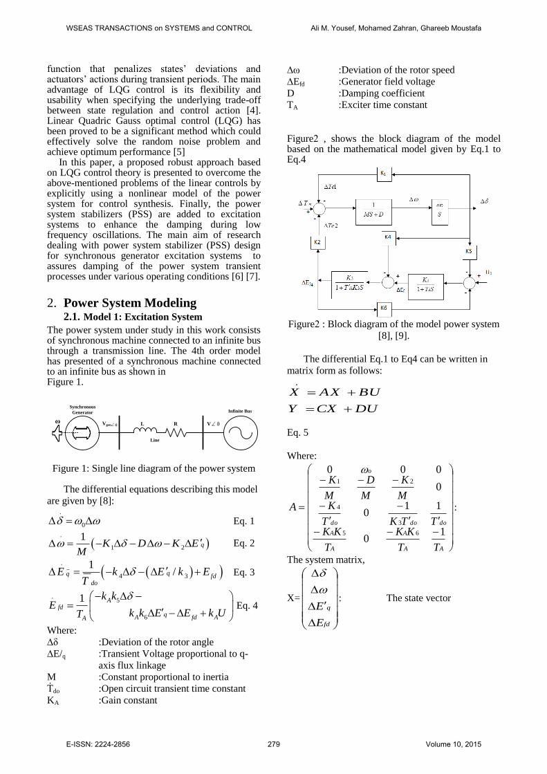
The power system under study in this work consists of synchronous machine connected to an infinite bus through a transmission line. The 4th order model has presented of a synchronous machine connected to an infinite bus as shown in Figure 1.
Synchronous
Generator Infinite Bus
Line
ω Vgen L R V
Figure 1: Single line diagram of the power system
The differential equations describing this model
are given by [8]: .
0 Eq. 1
.
1 2
1qK D K E
M Eq. 2
.
4 3
1/qq fd
do
E k E k ET
Eq. 3
.5
6
1 Afd
qA fd AA
k kE
k k E E k UT
Eq. 4
Where:
∆δ :Deviation of the rotor angle
∆E/q :Transient Voltage proportional to q-
axis flux linkage
M :Constant proportional to inertia
T do :Open circuit transient time constant
KA :Gain constant
∆ω :Deviation of the rotor speed
∆Efd :Generator field voltage
D :Damping coefficient
TA :Exciter time constant
Figure 2 , shows the block diagram of the model based on the mathematical model given by Eq.1 to Eq.4
Figure 2 : Block diagram of the model power system
[8], [9].
The differential Eq.1 to Eq4 can be written in
matrix form as follows: .
X AX BU
Y CX DU
Eq. 5
Where:
AA
A
A
A
dododo
o
TT
KK
T
KKTTKT
KM
K
M
D
M
K
A
10
110
0
000
65
3
4
21
:
The system matrix,
X=
fd
q
E
E
: The state vector
WSEAS TRANSACTIONS on SYSTEMS and CONTROL Ali M. Yousef, Mohamed Zahran, Ghareeb Moustafa
E-ISSN: 2224-2856 279 Volume 10, 2015
B=
A
A
T
K0
0
0
:
The input vector,
C 1 1 0 0 : The output vector
D 0 ,
U KX
The control signal
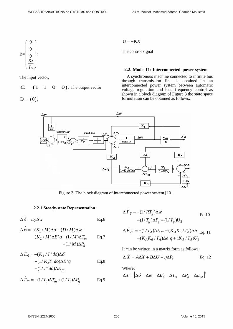
2.2. Model II : Interconnected power system
A synchronous machine connected to infinite bus through transmission line is obtained in an interconnected power system between automatic voltage regulation and load frequency control as shown in a block diagram of Figure 3 the state space formulation can be obtained as follows:
Figure 3: The block diagram of interconnected power system [10].
2.2.1. Steady-state Representation
.
o w Eq.6
.
1
2
( / ) ( / )
( / ) ' (1/ )
(1/ )
m
d
w K M D M w
K M E q M T
M P
Eq.7
.
4
3
( / ' )
(1/ ' ) '
(1/ ' )
q
fd
E K T do
K T do E q
T do E
Eq.8
.
(1/ ) (1/ )m t m t gT T T T P Eq.9
.
2
(1/ )
(1/ ) (1/ )
g g
g g g
P RT w
T P T U
Eq.10
.
5
6 1
(1/ ) ( / )
( / ) ' ( / )
fd A fd A A
A A A A
E T E K K T
K K T e q K T U
Eq. 11
It can be written in a matrix form as follows:
dPUBXAX .
Eq. 12
Where;
tfdgmq EPTEX '
WSEAS TRANSACTIONS on SYSTEMS and CONTROL Ali M. Yousef, Mohamed Zahran, Ghareeb Moustafa
E-ISSN: 2224-2856 280 Volume 10, 2015

t
g
A
At
T
T
K
B
BB
01
0000
00000
2
1
tUUU 21 Eq. 13
t
M
0000
10 Eq. 14
AA
A
A
A
gg
tt
dododo
TT
KK
T
KK
TRT
TT
TTKT
KMM
K
M
D
M
Kwo
A
1000
01
001
0
011
000
100
)(
10
001
00000
65
''
3
'
4
21
3. LQR Control Design Optimal control allows us to directly formulate the performance objectives of control system and produces the best possible control system for a given set of performance objectives. A control system which minimizes the cost associated with generating control inputs is called an optimal control system. The control energy can be expressed as U*R*U, where R is a positive definite square, symmetric matrix called the control cost matrix. Such an expression for control energy is called a quadratic form, because the scalar function, U*R*U, contains quadratic functions of the elements of U. Similarly, the transient energy can also be expressed in a quadratic form as XT*Q*X, where Q is a positive semi-definite square, symmetric matrix called the state weighting matrix [7]. The objective function can then be written as
follows:
0
J u T TX QX U RU dt
Eq. 15
The optimal control problem consists of solving
for the feedback gain matrix, K, such that the scalar
objective function, J(u), is minimized if all state
variables can be measured. Where, S is the positive definite matrix solution of the following control algebraic Riccati equation:
T 1 TSA A S Q S*B*R *B *S 0 Eq. 16
One of the important properties of LQ-regulators is that provided certain conditions are met, they
guarantee nominally stable closed-loop system. The conditions for achieving a stable LQ system are as follows:
R 0 , Q 0 .,
(A,B) controllable (stabilizable) .
[ , , ] ( , , , , )K S E lqr A B Q R N Eq. 17
Choosing the weight matrices Q and R usually involves some kind of trial and error, and they are usually chosen as diagonal matrices and N equal to zero.
4. Kalman Filter Design The Kalman filter approach provides us with a procedure for designing observers for multivariable plants. Such an observer is guaranteed to be optimal in the presence of noise signal. Since noise is rarely encountered, the power spectral densities used for designing the Kalman filter can be treated as tuning parameters to arrive at an observer for multivariable plants that has desirable properties, such as performance and robustness. Consider a plant with the following linear time-invarying state-space representation:
.
X AX BU w Eq. 18
Y CX DU v Eq. 19
Where;
w is the process noise vector
v is the measurement noise vector
For designing a control system, Therefore, an observer is required for estimating the state-vector, based upon a measurement of the output ,given by Eq.,s 18,19 and known input, U. Kalman filter is an optimal observer, which minimizes a statistical measure of the estimation error, eo=X-Xo , Where Xo is the estimated state-vector. The state-equation of the Kalman filter can be written as follows:
0 0 0* * *( * * )X A X B U L Y C X D U
Eq. 20
Where; L is the gain matrix of the Kalman filter.
T 1L S*C *Z Eq. 21
Since the Kalman filter is an optimal observer, the problem of Kalman filter is solved quite similarly to the optimal control problem. For the time-invariant problem, the following algebraic Reccati equation results for the optimal covariance matrix, [6] [7]:
T T 1 TA*S S*A –S*C *V *C*S B*W*B 0 Eq. 22
WSEAS TRANSACTIONS on SYSTEMS and CONTROL Ali M. Yousef, Mohamed Zahran, Ghareeb Moustafa
E-ISSN: 2224-2856 281 Volume 10, 2015

Where;
A, B, C, are the plant's state coefficient
matrices,
W is the process noise matrix,
V is the measurement noise matrix, and
S is the optimal covariance matrix of the
estimation error.
The algebraic Riccati equation can be solved using the specialized Kalman filter MATLAB command lqe. The Kalman filter optimal gain, L, is given by:
L,S,E lqe A,B,C,W,V Eq. 23
Where
L is the returned Kalman filter optimal gain,
S is the returned solution to the algebraic
Reccati equation, and
E is a vector containing the eigenvalues of the
Kalman filter (i.e. the eigenvalues of A-
LC).
5. LQG Controller Design If a controller is designed using the LQR, and the observer is designed using Kalman filter, the resulting system is referred to as Linear Quadratic Gaussian (LQG) Control or LQG-compensator. In short, the optimal compensator design process is the following [12]:
1. Design an optimal regulator for a linear plant
using full-state feedback. The regulator is
designed to generate a control input, u(t),
based upon the measured state-vector, X.
2. Design a Kalman filter for the plant assuming
a known control input, u(t), a measured
output, y(t), and white noises, w & v .
3. The Kalman filter is designed to provide an
optimal estimate of the state vector, X.
4. Combine the separately designed optimal
regulator and Kalman filter into an optimal
compensator (LQG), which generates the
input vector, u(t), based upon the estimated
state-vector, Xo ,rather than the actual state-
vector, X, and the measured output, y(t).
The measurement noise spectral density matrix, the state-space realization of the optimal compensator is given by the following state and output equations [7]:
0 oX = (A B*K L*C L*D*K)*X L*Y Eq. 24
oU K*X Eq. 25
Where K & L are the optimal regulator and Kalman
filter gain matrices, respectively, and
Xo is the estimated state vector.
Figure 3 shows the block diagram of the optimal LQG-compensator [7]. Using MATLAB's Control System Toolbox, a state-space model of the regulating closed-loop system, sysc; can be constructed as follows:
sysp ss A,B,C,D Eq. 26
A B*K L*Csysc=ss
L*D*K ,L ,K , zeros size D'
Eq. 27
syscl feedback(sysp,sysc) Eq. 28
Where sysp is the state-space model of the plant,
sysc is the state-space model of the LQG
compensator, and
syscl is the state-space model of the closed
loop system.
Figure 4: Block diagram of the optimal LQG-
compensator.
6. Simulation Results 6.1. Model I: Simulation Results
The dynamic stability of power system subjected to load disturbances by using the MATLAB program is proposed by choosing the machine parameters’ at nominal operating point [Active power P=1 pu, Reactive power Q=.25 pu].The LQG-controller will applied on the two models of the power system under study. The data sheet of the synchronous machine is given by [8] :
d q dd
do
o A A
X 1.6, X 1.55, X 0.32,
Xe 0.4,E 1, T 6,M 10,
377, D 0,K 25, T 0.06
The state coefficient matrices A, B of the 4th order plant with the given data sheet of synchronous
WSEAS TRANSACTIONS on SYSTEMS and CONTROL Ali M. Yousef, Mohamed Zahran, Ghareeb Moustafa
E-ISSN: 2224-2856 282 Volume 10, 2015
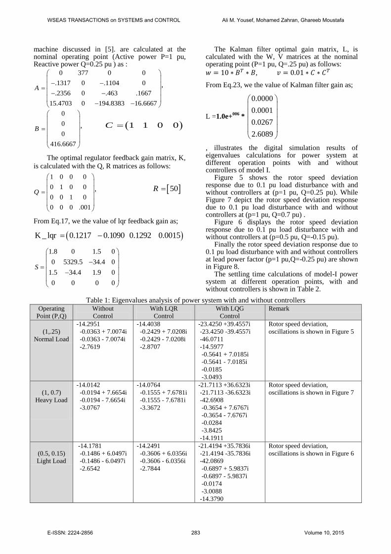
machine discussed in [5]. are calculated at the nominal operating point (Active power P=1 pu, Reactive power Q=0.25 pu ) as :
0 377 0 0
.1317 0 .1104 0
.2356 0 .463 .1667
15.4703 0 194.8383 16.6667
A
,
0
0
0
416.6667
B
, 1 1 0 0C
The optimal regulator feedback gain matrix, K,
is calculated with the Q, R matrices as follows:
1 0 0 0
0 1 0 0
0 0 1 0
0 0 0 .001
Q
, 50R
From Eq.17, we the value of lqr feedback gain as;
K _ lqr 0.1217 0.1090 0.1292 0.0015
1.8 0 1.5 0
0 5329.5 34.4 0
1.5 34.4 1.9 0
0 0 0 0
S
The Kalman filter optimal gain matrix, L, is calculated with the W, V matrices at the nominal operating point (P=1 pu, Q=.25 pu) as follows:
,
From Eq.23, we the value of Kalman filter gain as;
L =1.0e+006
*
0.0000
0.0001
0.0267
2.6089
, illustrates the digital simulation results of eigenvalues calculations for power system at different operation points with and without controllers of model I. Figure 5 shows the rotor speed deviation response due to 0.1 pu load disturbance with and without controllers at (p=1 pu, Q=0.25 pu). While Figure 7 depict the rotor speed deviation response due to 0.1 pu load disturbance with and without controllers at (p=1 pu, Q=0.7 pu) . Figure 6 displays the rotor speed deviation response due to 0.1 pu load disturbance with and without controllers at (p=0.5 pu, Q=-0.15 pu). Finally the rotor speed deviation response due to 0.1 pu load disturbance with and without controllers at lead power factor (p=1 pu,Q=-0.25 pu) are shown in Figure 8. The settling time calculations of model-I power system at different operation points, with and without controllers is shown in Table 2.
Table 1: Eigenvalues analysis of power system with and without controllers Operating
Point (P,Q)
Without
Control
With LQR
Control
With LQG
Control
Remark
(1,.25)
Normal Load
-14.2951
-0.0363 + 7.0074i
-0.0363 - 7.0074i
-2.7619
-14.4038
-0.2429 + 7.0208i
-0.2429 - 7.0208i
-2.8707
-23.4250 +39.4557i
-23.4250 -39.4557i
-46.0711
-14.5977
-0.5641 + 7.0185i
-0.5641 - 7.0185i
-0.0185
-3.0493
Rotor speed deviation,
oscillations is shown in Figure 5
(1, 0.7)
Heavy Load
-14.0142
-0.0194 + 7.6654i
-0.0194 - 7.6654i
-3.0767
-14.0764
-0.1555 + 7.6781i
-0.1555 - 7.6781i
-3.3672
-21.7113 +36.6323i
-21.7113 -36.6323i
-42.6908
-0.3654 + 7.6767i
-0.3654 - 7.6767i
-0.0284
-3.8425
-14.1911
Rotor speed deviation,
oscillations is shown in Figure 7
(0.5, 0.15)
Light Load
-14.1781
-0.1486 + 6.0497i
-0.1486 - 6.0497i
-2.6542
-14.2491
-0.3606 + 6.0356i
-0.3606 - 6.0356i
-2.7844
-21.4194 +35.7836i
-21.4194 -35.7836i
-42.0869
-0.6897 + 5.9837i
-0.6897 - 5.9837i
-0.0174
-3.0088
-14.3790
Rotor speed deviation,
oscillations is shown in Figure 6
WSEAS TRANSACTIONS on SYSTEMS and CONTROL Ali M. Yousef, Mohamed Zahran, Ghareeb Moustafa
E-ISSN: 2224-2856 283 Volume 10, 2015

(1, -0.25)
Lead PF
-14.9002
0.1021 + 6.3167i
0.1021 - 6.3167i
-2.4336
Un-stable
-15.0445
-0.2068 + 6.3348i
-0.2068 - 6.3348i
-2.2966
--25.0515 +42.0976i
-25.0515 -42.0976i
-49.3002
-15.2945
-0.6953 + 6.3571i
-0.6953 - 6.3571i
-0.0131
-2.0707
Rotor speed deviation,
oscillations is shown in Figure 8
Table 2, Settling time for single machine model with and without controllers
Without Control LQR- Control LQG- Control
P=1, Q=0.25 pu. Normal load > 10 Sec. > 10 Sec. 6.5 Sec.
P=1, Q=0.7 pu., Heavy load > 10 Sec. > 10 Sec. 9 Sec.
P=0.5, Q=0.15 pu. Light load > 10 Sec. 9 Sec. 5.5 Sec.
P=1, Q= -0.25 pu. Lead P.F. load
> 10 Sec 4 Sec.
Figure 5 : Rotor speed dev. response due to 0.1 pu load
distorbance with and without controllers, at (p=1 pu ,
Q=.25 pu ).
Figure 6: Rotor speed dev. response due to 0.1 pu load
distorbance with and without controllers at lead power
factor load (p=1.1 pu , Q=-.3 pu ).
Figure 7: Rotor speed dev. response due to 0.1 pu load
distorbance with and without controllers at (p=1.1 pu ,
Q=.75 pu ).
Figure 8 : Rotor speed dev. response due to 0.1 pu load
distorbance with and without controllers at lead power
factor load (p=1.1 pu , Q=-.82 pu ).
6.2. Model II: Simulation Results
The following mathematical linearized state
space model represents a power system which
consists of synchronous machine connected to
infinite bus through transmission line [9], [10]; The
block diagram is shown in Figure 3. Choosing the
machine parameters and nominal operating point as;
/
1.6; 1.55;
0.32; 0.4 .
d q
ed
X X
X X p u
0 1 2 3 4 5 6 7 8 9 10-1
-0.5
0
0.5
1
1.5x 10
-3
time in Sec.
Roto
r S
peed d
ev.
in
pu.
Rotor Speed dev. response in pu. at (P=1,Q= 0.25 pu.)
W/O -CONTROL
LQR-control
LQG - CONTROL
0 1 2 3 4 5 6 7 8 9 10-8
-6
-4
-2
0
2
4
6
8
10
12x 10
-4
time in Sec.
Roto
r S
peed d
ev.
in
pu.
Rotor Speed dev. response in pu. at (P=0.5,Q= 0.15 pu.)
W/O -CONTROL
LQR-control
LQG - CONTROL
0 1 2 3 4 5 6 7 8 9 10-6
-4
-2
0
2
4
6
8
10x 10
-4
time in Sec.
Roto
r S
peed d
ev.
in
pu.
Rotor Speed dev. response in pu. at (P=1,Q= 0.7 pu.)
W/O -CONTROL
LQR-control
LQG - CONTROL
0 1 2 3 4 5 6 7 8 9 10-4
-3
-2
-1
0
1
2
3
4x 10
-3
time in Sec.
Roto
r S
peed d
ev.
in
pu.
Rotor Speed dev. response in pu. at (P=1,Q= -0.25 pu.)
W/O -CONTROL
LQR-control
LQG - CONTROL
WSEAS TRANSACTIONS on SYSTEMS and CONTROL Ali M. Yousef, Mohamed Zahran, Ghareeb Moustafa
E-ISSN: 2224-2856 284 Volume 10, 2015

0 0377; 10; 6;
0; 0.06;
25( 1; 0.25);
0.08; 1.82; 0
d
A
A
t
M T
D T
K P Q
T R re
From LQR control (Eq. 17), the feedback gain and solution of Reccati equation are:
0.0265 -0.3333 -0.0390 0.0507 -0.0144 0.0037
0.0212 -0.2213 0.0740 0.0003 -0.0229 0.1461LQRK
From LQG and Kalman filter control (Eqn. 23), the observer gain matrix L and solution of reccati equation P are:
0.0000 0.0000 0.0000 0.0000 -0.0036 -0.0007
1.0e+9 * -5.0807 -0.6302 0.0000 0.0000 -0.0001 -0.0000
L
0.0000 0.0000 -0.0000 -0.0000 0.0000 -0.0000
0.0000 0.0000 -0.0000 -0.0000 0.0000 -0.0000
-0.0000 -0.0000 0.0000 0.0004 0.0000 -0.00001.0e+11*
-0.0000P
-0.0000 0.0004 1.1742 0.0000 -0.0001
0.0000 0.0000 0.0000 0.0000 0.0000 -0.0000
-0.0000 -0.0000 -0.0000 -0.0001 -0.0000 0.0000
Figure 9 shows the rotor angle deviation response due to 0.1 load disturbance with and without LQG and LQR controllers at lag power factor load (P=1, Q=0.25 pu). Figure 10 depicts the rotor speed deviation response due to 0.1 load disturbance with and without LQG and LQR controllers at lag power factor load (P=1, Q=0.7 pu). Figure 11 shows the rotor speed deviation response due to 0.1 load disturbance with and without LQG and LQR controllers at lead power factor load (P=0.5, Q= 0.15 pu) , Figure 12 shows the rotor speed deviation response due to 0.1 load disturbance with and without LQG and LQR controllers at lead power factor load (P=1, Q= -0.25 pu). Moreover, Table 3 shows the Settling time for single machine model with and without controllers at different operating conditions. Table 4 displays the Eigenvalues calculation with and without controllers for single machine power system.
Table 3, Settling time for single machine model with and without controllers
Operating points Without Control LQR- Control LQG- Control
P=1, Q=0.25 pu. Normal load > 10 Sec. > 10 Sec. 6 Sec.
P=1, Q=0.7 pu. Heavy load > 10 Sec. > 10 Sec. 9.5 Sec.
P=0.5, Q=0.15 pu. Light load > 10 Sec. > 10 Sec. 8 Sec.
P=1, Q= -0.25 pu. Lead P.F. load > 10 Sec 3 Sec.
Table 4: Eignvalues calculation with and without controllers of single machine power system Operating
point (P,Q)
Without
control
With LQR
control
With LQG
control
remark
(1,.25)
Normal Load
-0.0367 + 6.9961i
-0.0367 - 6.9961i
-14.2953
-12.4821
-2.7625
-3.7201
-36.9779
-14.2321
-0.1110 + 7.0260i
-0.1110 - 7.0260i
-1.1061
-3.7466
1.0e+002 *
-3.5443 + 3.1680i
-3.5443 - 3.1680i
-3.5623
-0.9704 + 3.1207i
-0.9704 - 3.1207i
-0.0017 + 0.0704i
-0.0017 - 0.0704i
-0.1423
-0.1250
-0.0019
-0.0377
-0.0371
Rotor speed deviation,
oscillations is shown in Figure
9
WSEAS TRANSACTIONS on SYSTEMS and CONTROL Ali M. Yousef, Mohamed Zahran, Ghareeb Moustafa
E-ISSN: 2224-2856 285 Volume 10, 2015

(1, 0.7)
heavy load
-0.0204 + 7.6552i
-0.0204 - 7.6552i
-14.0144
-12.4829
-3.7181
-3.0771
-36.8864
-14.2317
-0.0684 + 7.6758i
-0.0684 - 7.6758i
-1.2742
-3.7555
1.0e+002 *
-3.3674 + 3.0526i
-3.3674 - 3.0526i
-3.5144
-0.8119 + 2.9637i
-0.8119 - 2.9637i
-0.0011 + 0.0768i
-0.0011 - 0.0768i
-0.1423
-0.1250
-0.0033
-0.0378
-0.0371
Rotor speed deviation,
oscillations is shown in Figure
10
(0.5, 0.15)
Light Load
-0.1479 + 6.0363i
-0.1479 - 6.0363i
-14.1778
-12.4819
-2.6593
-3.7186
-36.9221
-14.2328
-0.1549 + 6.0546i
-0.1549 - 6.0546i
-1.0961
-3.7238
1.0e+002 *
-3.3246 + 3.0248i
-3.3246 - 3.0248i
-3.5016
-0.7765 + 2.9261i
-0.7765 - 2.9261i
-0.0016 + 0.0607i
-0.0016 - 0.0607i
-0.1423
-0.1250
-0.0025
-0.0375
-0.0372
Rotor speed deviation,
oscillations is shown in Figure
11
(1, -0.25)
Lead PF
0.1033 + 6.3047i
0.1033 - 6.3047i
-14.9008
-12.4804
-2.4303
-3.7285
Unstable
-37.2057
-14.2319
-0.1060 + 6.3558i
-0.1060 - 6.3558i
-3.7440
-0.8909
1.0e+002 *
-3.7002 + 3.2728i
-3.7002 - 3.2728i
-3.5988
-1.1326 + 3.2653i
-1.1326 - 3.2653i
-0.0027 + 0.0638i
-0.0027 - 0.0638i
-0.1423
-0.1250
0.0003
-0.0376
-0.0371
Rotor speed deviation,
oscillations is shown in Figure
12
Figure 9: Rotor angle dev. Response due to 0.1 load
disturbance with and without LQG and LQR controllers at lag power factor load (P=1, Q=0.25
pu)
Figure 10: Rotor speed dev. Response due to 0.1
load disturbance with and without LQG and LQR
controllers at lag power factor load (P=1, Q=0.7 pu)
0 1 2 3 4 5 6 7 8 9 10-1
-0.5
0
0.5
1
1.5x 10
-3
time in Sec.
Mechanic
al to
rque d
ev.
in p
u.
Rotor speed dev. (P=1,Q= 0.25pu.)
W/O -CONTROL
LQR-control
LQG - CONTROL
0 1 2 3 4 5 6 7 8 9 10-6
-4
-2
0
2
4
6
8
10x 10
-4
time in Sec.
Mechanic
al to
rque d
ev.
in p
u.
Rotor speed dev. (P=1,Q= 0.7pu.)
W/O -CONTROL
LQR-control
LQG - CONTROL
WSEAS TRANSACTIONS on SYSTEMS and CONTROL Ali M. Yousef, Mohamed Zahran, Ghareeb Moustafa
E-ISSN: 2224-2856 286 Volume 10, 2015

Figure 11: Rotor speed dev. Response due to 0.1
load disturbance with and without LQG and LQR
controllers at lead power factor load (P=0.5,
Q=0.15 pu)
Figure 12: Rotor speed dev. Response due to 0.1
load disturbance with and without LQG and LQR
controllers at lead power factor load (P=0.5,
Q=0.15 pu)
7. Discussions The simulation results of Model I show the effect of the proposed LQG controller for damping the dynamic oscillation on power system in a wide range of operating conditions. The power system understudy at the operating points (1,-0.25) is un-stable system in case of without control as shown in Figures 8, 12. After the effect of the control based on LQR the system became stable. Moreover, after the effect of the proposed control based on LQG, the system became fast damping at all operating points see the eigenvalues in Tables 1,2,3,4. Also, Tables 2, 4 shows the settling time in case of proposed LQG controller is less than that in case of LQR controller at all operating conditions.
8. Conclusion This paper presented a proposed robust controller based on Linear Quadratic Gaussian LQG theory to design a power system stabilizer for single-machine infinite-bus power systems. The proposed approach overcomes the problems of the linear controls by explicitly using a nonlinear model of the power system for control synthesis. The proposed robust linear quadratic Gaussian control LQG-PSS is design and applicator of the power system under study. The comparison shows that the proposed robust LQG controller is effective and robust in suppressing large disturbances, as well as enhancing the power system stability. It is also suitable for a wide range of operating conditions of the power system compared with the conventional linear quadratic control LQR-PSS. The LQG optimal control has been developed to be included in power system in order to improve the dynamic response and gives the optimal performance at any loading condition. The LQG is better than LQR controller in terms of small settling time and less overshoot and under shoot. The digital simulation results show that the proposed PSS based
upon the LQG can achieve good performance over a wide range of operating conditions.
Bibliography
[1] N.K. Roy, H.R. Pota, and M.A. Mahmud,
"Design of a Norm-Bounded LQG Controller
for Power Distribution Networks with
Distributed Generation," 2012 Australian
Control Conference, 15-16 November 2012,
Sydney, Australia.
[2] Argyrios C. Zolotas, Balarko Chaudhuri, Imad
M. Jaimoukha, and Petr Korba, "A Study on
LQG/LTR Control for Damping Inter-Area
Oscillations in Power Systems," IEEE
TRANSACTIONS ON CONTROL SYSTEMS
TECHNOLOGY, VOL. 15, NO. 1, JANUARY
2007.
[3] Ibraheem K. Ibraheem, " Damping Low
Frequency Oscillations in Power System using
Quadratic Gaussian Technique based Control
System Design," International Journal of
Computer Applications (0975 – 8887), Volume
92 – No.11, April 2014.
[4] Xuejiao Yang and Ognjen Marjanovic, "LQG
Control with Extended Kalman Filter for
Power Systems with Unknown Time-Delays,"
Preprints of the 18th IFAC World Congress,
Milano (Italy) August 28 - September 2, 2011.
[5] Qi-bing JIN,Shi-bing REN, Ling Quan, "LQG
Optimum Controller Design and Simulation
Base on Inter Model Control Theory," 978-1-
4244-4738-1/09/$25.00 ©2009 IEEE..
[6] S.S. Lee and J.K. Park, "Design of reduced-
0 1 2 3 4 5 6 7 8 9 10-8
-6
-4
-2
0
2
4
6
8
10
12x 10
-4
time in Sec.
Mechanic
al to
rque d
ev.
in p
u.
Rotor speed dev. (P=0.5,Q= 0.15pu.)
W/O -CONTROL
LQR-control
LQG - CONTROL
0 1 2 3 4 5 6 7 8 9 10-4
-3
-2
-1
0
1
2
3
4x 10
-3
time in Sec.
Mechanic
al to
rque d
ev.
in p
u.
Rotor speed dev. (P=1,Q= -0.25pu.)
W/O -CONTROL
LQR-control
LQG - CONTROL
WSEAS TRANSACTIONS on SYSTEMS and CONTROL Ali M. Yousef, Mohamed Zahran, Ghareeb Moustafa
E-ISSN: 2224-2856 287 Volume 10, 2015

order observer-based variable structure power
system stabiliser for unmeasurable state
variables," IEE Proceedings of the Generation,
Transmission and Distribution, vol. 145, No. 5
(September 1998), pp. 525–530.
[7] Ashish Tewari, "Modern Control Design With
Matlab And Simulink," Book-2003..
[8] M.K. El-Sherbiny, M.M. Hasan, G. El-Saady,
Ali M. Yousef, "Optimal pole shifting for
power system stabilization," Electrical power
system research journal, No 66 pp.253-
258,2003..
[9] Ali M. Yousef, Ahmed M. Kassem, " Optimal
Power System Stabilizer Based Enhancement
of Synchronizing And Damping Torque
Coefficients," WSEAS TRANSACTIONS on
POWER SYSTEMS, Issue 2, Volume 7, April
2012.
[10] Ahmed Said Oshaba, " Stability of Multi-
Machine Power System by used LQG
Controller," WSEAS TRANSACTIONS on
POWER SYSTEMS, Volume 9, 2014.
WSEAS TRANSACTIONS on SYSTEMS and CONTROL Ali M. Yousef, Mohamed Zahran, Ghareeb Moustafa
E-ISSN: 2224-2856 288 Volume 10, 2015
Top Related