


Languages
Pages
Legal

Implied Variance and Market Index Reversal
Christopher S. JonesMarshall School of Business
University of Southern [email protected]
Sung June PyunMarshall School of Business
University of Southern [email protected]
Tong WangPamplin College of BusinessVirginia Tech University
March 2016
Abstract
We find that the S&P 500 Index, its futures contracts, and its most popular ETF displaystrong evidence of daily return reversal when implied variance is high. This negative serialcovariance is mostly observed following negative market returns, while positive returns showa moderate tendency to continue when implied variances are high. Price changes around theclose and the open show a somewhat stronger tendency to reverse, though the serial covariancewe document generally takes longer than a day to resolve. Furthermore, reversal tend to bestronger when option open interest is high, and the presence of return reversal has a significanteffect on the performance of option trading strategies. Our results have important implicationsfor how market participants interpret implied variances, which due to serial covariance providean extremely biased forecast of longer-horizon return variances.
JEL classification: G12, G13, G14.
Keywords: Implied volatility, return reversal, liquidity.
1

1 Introduction
Option markets have the potential to provide extremely useful information to investors, even those
who are not interested in trading options. An obvious example is an asset’s implied volatility,
which may be valuable to an investor making a risk/reward calculation involving that asset. A
precondition is that the implied volatility is reasonably correlated with actual return volatility, and
that any bias in implied volatility be stable and therefore correctable.
Starting with the studies of Day and Lewis (1992) and Lamoureux and Lastrapes (1993), the
empirical options literature has shown that implied variances from equity index options are highly
informative predictors of future realized variances.1 At the same time, they display a systematic
upward bias, and furthermore display a degree of variation that appears to be greater than that of
actual ex ante variance, results that may be interpreted as reflecting the existence of risk premia on
jumps and/or volatility. Fortunately, under plausible assumptions this bias can be well captured
by a simple linear adjustment, as Chernov (2007) demonstrates empirically.
Evaluation of implied volatility forecasts have, since the inception of this literature, generally
evaluated those forecasts on the basis of their ability to predict variances computed from all daily
returns realized over the remaining life of the option. This choice is natural. Since the seminal
work of Merton (1980), it has been well known that higher frequency data can be used to construct
a more accurate proxy of a latent volatility process. Thus, forecast evaluation using daily realized
variances should provide far more power than, say, forecasting the squared monthly return. Forecast
evaluation based on realized variances computed from intra-day returns, an approach used by Blair
et al. (2001), in theory has even greater informativeness, though microstructure issues complicate
implementation and interpretation.
Under the assumption that returns are serially uncorrelated, a variance forecast that is con-
structed be an unbiased predictor of realized variance from daily returns will offer a similarly
unbiased forecast of monthly return variance. This is important given that many uses of variance
1Somewhat contradictory evidence was presented by Canina and Figlewski (1993), who found that implied vari-
ances are essentially uncorrelated with future realized variances. The unrepresentative result of this paper is explained
by Christensen and Prabhala (1998).
1

forecasts, for example in portfolio optimization, require that the variance forecast’s horizon corre-
spond to the anticipated holding period. Traditionally, this assumption has been accepted without
very much scrutiny.
There is a long list of studies, however, that challenge the assumption of zero autocorrelation.
One set focuses on the finding of positive index autocorrelation, first identified by Lo and MacKinlay
(1988) and Conrad and Kaul (1988) in studies of the CRSP market index. Campbell et al. (1993)
observed that the autocorrelation was decreasing in the level of trading volume. They further
hypothesized that autocorrelation should decrease with volatility, which was confirmed by LeBaron
(1992).
The difficulty in interpreting these results is that they could be due to the effects of asynchronous
prices, whereby the closing prices of different securities are indicative of values at different points
in time. This has been shown by Fisher (1966) to produce spurious autocorrelation at the index
level even when individual security returns are serially independent, and it is consistent with the
finding from these papers that autocorrelations are smaller in value weighted portfolios than in
equally weighted portfolios, which put more weight on stocks whose closing prices are more likely
to be stale. Furthermore, Ahn et al. (2002) show that the positive autocorrelations observed in
the so-called ‘cash’ market indexes are largely absent from futures returns, again suggesting that
serial correlation is likely a figment of microstructure effects and not something that is in any way
exploitable by traders.
More recently, however, a group of studies has documented new evidence of serial correlation in
stock market returns, but in this case the autocorrelation is negative and therefore inconsistent with
stale prices. Bates (2012), for example, reports that the value weighted CRSP portfolio displayed
significantly negative autocorrelations for several years during the U.S. Financial Crisis. Etula
et al. (2015) find strong evidence of short-term return reversals in U.S. and international stock
market indexes around the end of the month, a pattern that they attribute to the concentration
of institutional trading at that time. Chordia et al. (2002) demonstrate that aggregate order
imbalances, which are positively correlated with contemporaneous returns, negatively predict next-
day market returns. Ben-Rephael et al. (2011) show that daily flows in mutual funds generate a
2

similar pattern of reversal in the Israeli stock market.
The primary goal of our paper is to reassess the ability of implied variances of S&P 500 Index
options to forecast future realized variances at different horizons. Specifically, we are interested in
whether implied variances are as useful in forecasting longer-horizon (e.g. monthly) realized variance
as they are in forecasting short-run (e.g. daily) variances, where any difference is attributable to
the presence of serial correlation.
Our main result is that the VIX index, a measure of the implied variance of the S&P 500 Index,
is a much more biased forecast of longer-horizon variance than it is of the short-horizon variances
typically examined. Specifically, in regressions in which implied variance is the sole predictor, the
slope coefficient in a regression in which the dependent variable is the monthly squared return is less
than half the coefficient of a regression in which the dependent variable is the sum of squared daily
returns. Because the difference between these two dependent variables is a measure of inter-day
serial covariance, these results are equivalent to a finding that serial covariance is predictable by
implied variance. The predictability of serial covariance is highly significant.
This result is very robust. Similar results are obtained for the cash index, the S&P 500 futures
contract, and the SPY “Spider” ETF, suggesting that reversal-based trading strategies may be
implementable, depending on transactions costs. We find similar and significant results in both
halves of our sample, meaning that a single episode, such as the Financial Crisis, is not responsible
for our findings. Finally, we find predictable reversal using different measures of implied variances,
based on the Black-Scholes model and on a ‘model-free’ approach.
It is worth emphasizing that the serial covariance we are documenting is negative rather than
positive. In addition, our primary focus is on the S&P 500 Index futures market rather than a cash
index. Thus, our findings are fundamentally different from those of Lo and MacKinlay (1988) and
LeBaron (1992), for example, who may primarily be documenting patterns in the staleness of prices
that imply spuriously positive autocovariance as a result of the bias identified by Fisher (1966).
We further show that most autocovariance is the result of the reversal of negative rather than
positive returns. That is, as implied variances increase, a negative return is much more likely to
be reversed in the next day or more, while positive returns are not. This raises the possibility that
3

either market liquidity is asymmetric, able to absorb buy orders with less transitory price impact
than sell orders, or that available liquidity is symmetric but more likely to be overwhelmed by
selling pressure, for example from fire sale-type trades.
These results are complementary to recent work showing that the VIX is related to market
liquidity. Most notably, Nagel (2012) shows that the level of the VIX is strongly positively related
to the profitability of the short-run reversal strategies of Lehmann (1990) and Lo and MacKinlay
(1990). Interestingly, while reversal trading has typically been most profitable in small, illiquid
stocks (see Avramov et al., 2006), Collin-Dufresne and Daniel (2015) find significant evidence of
reversal in the largest U.S.-listed stocks, but they see no relation between large-cap reversal returns
and the VIX index.
Our results are notable in that they provide an additional link between the VIX index and mar-
ket liquidity and substantially strengthen earlier findings by showing strong evidence of recurrent
negative autocorrelation at the index level. Our results are also somewhat unique in showing that
return reversal remains a significant force even in the last two decades, during which the returns to
traditional cross-sectional reversal strategies have been steadily declining (see Khandani and Lo,
2007).
Our second set of results concerns the exact timing of reversal. We see evidence of reversal in
daily close-to-close returns, but is that where the tendency to reverse is strongest? To answer this
question, we examine daily returns formed based on prices observed at times of day other than
the close. We find that reversal based on closing prices is indeed stronger than reversal based on
prices at most other times of the day. The exception is that reversal is particularly strong when
daily returns are based on prices immediately after the open. Regardless of the time at which daily
prices are recorded, autocovariances are more negative when implied variances are high. The effect
is not particularly strong for returns based on closing prices.
We also examine reversal over horizons shorter than a day. Specifically, we look at how returns
over the last N minutes of one day are reversed in the time from that day’s close to N minutes
after the next day’s open. We find that reversal is strongest for N between about 20 and 60.
Furthermore, this very short-term reversal is most sensitive to the level if implied variance is above
4

average. When implied variances are high, futures price movements in the last 30 minutes or so
of the day have a very strong tendency to reverse during the overnight periods and the first 30
minutes of trading the following morning.
In light of the finding that returns around the end of the day seem to exhibit greater reversal,
particularly when implied variances are high, we examine a potential explanation. Specifically, we
hypothesize that end-of-day hedging by options traders may cause temporary price dislocation in
the market index. We therefore investigate the relationship between reversal and the level of open
interest in S&P 500 Index options. We find that the VIX forecasts negative future autocovariance
more strongly when this open interest is high. This result is obtained both for raw open interest
and for a detrended measure of open interest.
Our final set of results concerns implications for option trading strategies. As shown by Lo
and Wang (1995), the fact that asset prices are discounted martingales under the risk neutral
distribution means that option prices are unaffected by serial correlation – under the risk neutral
distribution, it does not exist. As a result, at least in theory, option prices should be more closely
related to daily return volatility than to monthly return volatility, which is impacted much more
heavily by serial correlation. At the same time, the expected payoff of the option is determined by
the actual distribution of returns, which does depend on serial correlation. Hence serial correlation
has a potentially important role to play in determining expected option returns.
The option strategy we focus on is the at-the-money straddle on the S&P 500 Index. This
combination of an at-the-money put and an at-the-money call is constructed to have zero delta,
so that it represents a bet not on the direction of prices but rather on the absolute value of their
change, i.e. it is a bet on volatility. Negative autocorrelation in the returns on the underlying asset
decreases the volatility of the underlying price at longer horizons, and hence reduces the expected
payoff of the straddle. Since the prices of the call and put are not reduced by that autocorrelation,
the result of negative autocorrelation should be lower average returns on the straddle.
For the straddle buyer, there is a natural way to avoid this trap, which is to rebalance the
portfolio daily such that at the end of every day the trader again holds an at-the-money zero delta
straddle. This works by making the trader, at the end of each trading day, indifferent as to whether
5

the next day’s underlying price change is positive or negative, implying that they are protected
from the effects of return reversal.
We examine the returns on these two versions of the straddle trade, as well as the difference
in those returns, for straddles of one, two, and three months until expiration. On average, we find
that the buy-and-hold strategy underperforms the daily rebalanced strategy, reflecting the fact that
serial covariance is on average negative. However, these differences are not significant. When we
regress the difference between the buy-and-hold and rebalanced returns on implied variance, we find
a significant relation. When implied variance rises, serial covariance drops, and the buy-and-hold
strategy substantially underperforms the rebalanced strategy.
Taken together, the evidence presented in this paper shows that even the most liquid assets
display serial correlation in high uncertainty environments. The effect is not small. It leads to a
striking reinterpretations of what a change in implied variance actually means for investors, and
it has considerable implications for how equiy and option traders should behave in the midst of a
volatile market.
2 Variance and covariance forecasts
2.1 Regression framework
Traditionally, the literature examining implied variances as forecasts of future realized variances
has focused on the following specification:
Nt∑i=1
r2i,t = αd + βdIVt−1 + εd,t (1)
In this regression, ri,t represents the logarithmic return of an asset on day i of month t minus the
contemporaneous riskless return. Nt is the number of trading days within that month, and IVt−1
is the implied variance of the asset at the end of the prior month.2
In this paper, we propose to also examine the regression based on squared monthly excess
2As a test of predictability in variances, the regression suffers from a slight misspecification because returns are
not demeaned. It has been understood at least since French et al. (1987) that demeaning has very little impact on
squared returns. We will return to this issue later to show that it is not affecting any of our results materially.
6

returns, (Nt∑i=1
ri,t
)2
= αm + βmIVt−1 + εm,t, (2)
which follows from our use of continuously compounded excess returns, which at the monthly level
are sums of daily values. Because (Nt∑i=1
ri,t
)2
=
Nt∑i=1
Nt∑j=1
ri,trj,t,
we can decompose the monthly squared excess return as follows:(Nt∑i=1
ri,t
)2
=
Nt∑i=1
r2i,t + 2
Nt−1∑i=1
Nt∑j=i+1
ri,trj,t. (3)
Aside from expected return effects, which will be small, the second term can be interpreted as a mea-
sure of serial covariance, while the first term is simply the sum of squared daily returns considered
above. Thus, the wedge between daily and monthly realized variance is inter-day autocovariance.
We compile several different series for each dependent and independent variable. Daily returns
are based on closing prices of the S&P 500 ‘cash’ Index, the front month S&P 500 futures contract,
or the SPY exchange traded fund, which is the oldest and largest ETF tracking the S&P 500 Index.
The riskless rate we use is from Kenneth French’s website.
Our independent variable is usually based on the VIX, which is the Volatility Index constructed
by the Chicago Board Options Exchange (CBOE). The VIX a model-free implied volatility con-
structed similarly to that proposed by Britten-Jones and Neuberger (2000), and its construction
involves interpolation such that the measure can be interpreted as corresponding to a one-month
contract. In some cases we use the VXO instead. This is a predecessor of the VIX index that is
based on the Black-Scholes model and is constructed from options on the S&P 100 Index.
We create a rescaled measure of implied variance as
IVt =VIX2
t
120,000, (4)
where VIX is replaced by VXO in some cases. The denominator reflects the conversion of percentage
to decimal and annual to monthly, so that the resulting series is comparable to our realized variances.
Table 1 contains summary statistics for the data that will underlie most of the analysis in this
section. All data in the table are monthly. The sum of squared daily returns is the dependent vari-
7

able of regression (1), while the monthly squared return is the dependent variable of (2). Following
(3), we define the difference as the latter minus the former. The table also shows the end-of-month
values of the squared and rescaled VIX index, computed as in (4).
Several patterns in the data are immediately apparent. First, the average sum of squared daily
returns exceeds the average monthly squared return by a significant margin. From (3), this implies
that serial covariances are negative on average.3 A second observations is that all variance proxies
are persistent, though the sum of squared daily returns is more persistent than the monthly squared
return. It is possible that the lower persistence of monthly squared returns is the result of more
noise in that measure, but if so this noise is not obvious from the standard deviations of the two
proxies, since monthly squared returns display less variability. The higher volatility of the sum
of squared daily returns could be related to the presence of significantly greater kurtosis in daily
returns. A final observation is that implied variances on average exceed both measures of realized
variance, a standard result that likely reveals the presence of a volatility risk premium.
2.2 Main results
We report the results of variance forecasting regressions (1) and (2) in Table 2. The left side of
the table contains results for regression (1), where the dependent variable is the sum of squared
daily returns, which is the the traditional specification for evaluating the bias and efficiency of
implied variance forecasts. Consistent with a large literature, the slope coefficient of the regression
is highly significant in all specifications, with substantial R-squares. The slope coefficients are also
all slightly less than one, which is also a common finding, though we cannot reject the unit slope.
The right side of the table reports results for regression (2), in which the dependent variable is
the squared monthly return. Results here are much different. In almost every sample, the slope
coefficient drops by at least half, in many cases more, indicating that the variance of monthly
returns is much less responsive to changes in implied variances. This pattern holds for the S&P
3As we discuss below, our variance measures use returns that are not demeaned, and hence there is a small
difference between the sum of squared daily returns and the monthly squared return that is driven by expected
returns. However, this component should increase the monthly squared return relative to the sum of squared daily
returns. Hence it cannot explain the average difference shown in the table.
8

500 Index, index futures, and the SPY ETF. It is present in our main sample period, in each half
of our sample, and in an extended sample. For the extended sample, we base our implied variance
measure on the VXO index rather than the VIX, since the former is available for four additional
years. Although regressions using the VXO are somewhat haphazard given that the dependent
variable is based on S&P 500 returns, while the independent variable is from S&P 100 options, the
results are nevertheless consistent with others. Furthermore, they show that the lower slope for
regression (2) is obtained in a period that includes the crash of 1987 and that it is found whether
we use model-free or Black-Scholes implied variances.
In comparing the two sets of results, we also see that the R-squares are usually much lower
for the monthly squared return regressions. This is to be expected. Since the work of Merton
(1980) and Andersen and Bollerslev (1998), it has been well understood that higher frequency
data contain significantly more information about the latent variance process and can be used to
construct much more powerful tests of the accuracy of variance forecasts. The monthly squared
return simply contains more noise, and as a result it cannot be predicted as reliably. The only
exception is for the extended sample, which includes the crash of 1987. This caused an enormous
outlier in daily squared returns, which was not as obvious in monthly returns.
For high frequency data to truly offer better inference they must be a proxy of the same latent
variance process, in that the variance rate of high-frequency returns be the same as that of low-
frequency returns. This is equivalent to stating that returns are serially uncorrelated.
To test for the predictability serial covariance directly, we use the result from (3) that a serial
covariance measure,
2
Nt−1∑i=1
Nt∑j=i+1
ri,trj,t, (5)
can be constructed from the difference between monthly and daily return variances. We refer to
this measure as ‘total autocovariance’ to emphasize that it is reflects all lead-lag relations between
daily returns within a given month.
Regressing total autocovariance on implied variance will yield a slope coefficient that is exactly
equal to βm − βd, the difference between the slopes of (2) and (1). Table 3 reports the results of
this regression, mainly to verify that the difference in slopes is statistically significant. In short,
9

we find very strong evidence, across all samples, that covariance decreases with the level of implied
variance.
As noted above, this is at first glance the result of LeBaron (1992), who also shows that higher
variance reduces autocorrelations in the market index. The subtle but crucial difference is that
we are showing that higher implied variances make autocovariance more negative, while LeBaron
demonstrated that higher variance makes positive autocorrelations closer to zero. Furthermore, the
positive autocorrelations documented by LeBaron are in the cash index in a sample that ends in
1988, which leads to the concern that the autocorrelations are spurious, resulting from the stale
price bias of Fisher (1966). The negative autocovariances we are attempting to explain cannot be
explained by stale prices, and furthermore are present in the returns of easily tradable securities.
The results we have documented so far have rather striking implications for longer-term in-
vestors. Specifically, they show that when the VIX rises, say from 15% to 20%, the annualized
conditional standard deviation implied by the daily squared return regression, estimated from fu-
tures returns, rises from about 11% to 17%. The conditional standard deviation implied by the
monthly squared return regression rises from about 11% to just 14%.4 In other words, about half of
the increase in short-run volatility is transitory, present in daily returns but not in monthly returns.
Figure 1 shows the full relation between the VIX index and the annualized standard deviations
of stock returns, implied by the futures-based estimates of regressions (1) and (2). Overall, while
it is apparent that neither relation is exactly linear, the sensitivity of daily return volatility to the
VIX is roughly twice that of monthly return volatility. The difference between the two is, over
most of the historical range of the VIX, highly economically significant.
The presence of transitory volatility mirrors earlier work such as Poterba and Summers (1988)
and Campbell and Viceira (2002) documenting the presence of a substantial mean reverting com-
ponent in stock prices and showing how this reduces the variance of long-term returns. Barberis
4The relation between VIX and the conditional standard deviation can be convex or concave, depending on the
values of the slope and intercept parameters. For the daily squared return regression, it is convex. For the monthly
squared return regression, it is concave. This explains why the conditional volatility forecast constructed from the
daily squared return regression can increase more than one-for-one with the VIX even though conditional variance
increases less than one-for-one.
10

(2000) shows that these transitory returns have a significant impact on the portfolio decisions of
long-horizon investors. Our results have similar implications, except that they concern horizons of
days or months rather than years or decades.
2.3 Mean effects
Our results thus far are based on a minimal set of assumptions. One that deserves some scrutiny
is that the difference between the dependence of daily and monthly squared returns on implied
variances is that they are differentially sensitive to changes in expected returns.
Suppose that the average daily excess return in month t is equal to µt. Then the sum of squared
daily returns can be rewritten as the sum of a true variance measure and a term driven by expected
returns:Nt∑i=1
r2i,t =
Nt∑i=1
(ri,t − µt)2 +Ntµ2t (6)
The squared monthly return is(Nt∑i=1
ri,t
)2
=
Nt∑i=1
Nt∑j=1
(ri,t − µt)(rj,t − µt) +N2t µ
2t
=
Nt∑i=1
(ri,t − µt)2 + 2
Nt−1∑i=1
Nt∑j=i+1
(ri,t − µt) (rj,t − µt) +N2t µ
2t ,
where the last three terms can be interpreted as a true short-run variance component, a true
covariance measure, and an expected return component.
What these expressions show is that serial covariances are not the only difference between the
daily and monthly variances. They also differ because of how they are each impacted by expected
returns. Specifically, the impact of the mean on squared monthly returns is Nt (the number of days
in month t) times bigger than its impact on the sum of daily squared returns. Thus, it is possible
that the differences between the results obtained in regressions (1) and (2) are due to expected
returns being dependent on implied variances.
There is a large literature, starting with French et al. (1987), examining whether variances
predict returns. Originally, the predictor was a measure of volatility from lagged returns. More
recently, some authors are using implied volatilities, e.g. the VIX index, as predictors. Results
11

from this literature are varied and appear to be sensitive to the sample periods and specifications.
While French et al. find little evidence of any relation between actual price volatility and future
market returns, some authors such as Bollerslev et al. (2015) find that expected long horizon market
returns do tend to be increasing in the VIX.
Table 4 investigates the possibility of a risk/return relation in our sample, reporting the results
of regressions of the formNt∑i=1
ri,t = α+ β f(IVt−1) + εt, (7)
where f(x) = x,√x, or 1/
√x. The dependent variable in all regressions is computed from daily
excess returns on S&P 500 Index futures, and the independent variable is based on either the VIX
or the VXO index. Sample periods are dictated by the availability of these volatility indexes.
In short, the table shows no evidence that implied variances are in any way related to expected
market returns. Thus, it seems almost impossible that any of our earlier results could have been
driven by mean effects. In addition, from a theoretical standpoint, a mean-based explanation of
our main results would have been unlikely. Our finding is that the slope from the regression based
on monthly returns is lower than that based on daily returns, i.e. βm < βd. For the low value
of βm to be attributable to a mean effect, it would have to be the case that µ2t was decreasing in
implied variance. This would require that mean returns be either very positive or very negative
when implied variances are low, moving closer to zero as implied variances rise. Since negative risk
premia are theoretically unlikely, this means that expected returns are decreasing in risk, which
is not only intuitively implausible but inconsistent with the handful of studies that find a positive
relation. All in all, we find little merit to the hypothesis that our findings are due to expected
returns varying with implied variances.
2.4 Covariance decompositions
In this section we examine the nature of the serial covariances that accompany high levels of
implied variance. We begin by decomposing the total autocovariance measure studied previously
12

into a first-order term and a higher-order term. In particular, we can write total autocovariance as
2
Nt−1∑i=1
Nt∑j=i+1
ri,trj,t = 2
Nt−1∑i=1
ri,tri+1,t + 2
Nt−2∑i=1
Nt∑j=i+2
ri,tri+1,t. (8)
The first term captures the covariance between adjacent days within the month. The second term
is a measure of all serial covariances at lags of two or more.
Table 5 shows the results of regressing each covariance component on implied variance. In short,
the table shows that both first-order and higher-order autocovariances are negatively related to the
level of implied variances. For most samples, the first order effect is more highly significant, but
with a smaller slope coefficient and a lower R-square. This indicates that the tendency for returns
to reverse when VIX is high is not exclusively a high-frequency phenomenon. There is substantial
evidence that more than a day is required for the reversal to occur.
That said, the effect of implied variances on first-order autocovariance is large when we take
into account that the standard deviation of the dependent variable in the first-order regression is
only about half that of the higher-order regression.5 Thus, even though the slope coefficient is
smaller in the first-order regression, implied variance nevertheless explains an important part of
realized first order autocovariances.
An alternative way to decompose covariance is to create a term that reflects reversal or contin-
uation following negative returns and another term that describes what happens following positive
returns. Specifically, we can write
2
Nt−1∑i=1
Nt∑j=i+1
ri,trj,t = 2
Nt−1∑i=1
Nt∑j=i+1
ri,trj,t1 (ri,t ≥ 0) + 2
Nt−1∑i=1
Nt∑j=i+1
ri,trj,t1 (ri,t < 0) , (9)
where 1(C) = 1 if condition C is true and 1(C) = 0 otherwise. If negative returns subsequently
reverse but positive returns continue, for example, then the first term will be positive and the
second term will be negative.
The results of regressing each of these two components on implied variance are presented in
Table 6. What emerges is a clear pattern in which higher implied variance predicts greater reversal
5The first-order covariance measure is on average the sum of about 20 elements. The higher-order covariance
sums about 190 elements on average. This would appear to be the natural explanation for the greater variance in
the higher-order covariance measure.
13

following negative returns. Higher implied variances do not predict stronger reversals following
positive returns, however. In fact, we see evidence that they instead push serial covariance towards
positive values. This effect is smaller but nevertheless significant in most samples.
In the literature on return reversal in individual stocks, reversal of positive and negative returns
has been viewed as potentially arising from different sources. Da et al. (2014), for example, argue
that liquidity shocks are the primary cause of the reversal of negative returns, while positive returns
reverse as the result of investor sentiment combined with short-sale constraints. Our findings there-
fore reinforce existing work, such as Nagel (2012), which concludes that higher implied variances
are an indicator of low liquidity.
The finding that autocovariances become positive at high levels of the VIX is surprising given
our evidence thus far.6 While earlier papers such as Lo and MacKinlay (1988) and Conrad and
Kaul (1988) found evidence of positive autocorrelation in returns, this evidence was limited to
cash indexes, which are subject to biases resulting from stale prices. In addition, as shown by
LeBaron (1992), positive autocorrelation was stronger when variances were low. Thus, our findings
on continuation of positive returns are novel in several respects.
3 Reversal timing
Thus far we have seen substantial evidence that serial covariance in daily returns is related to the
level of implied variances. In this section we start by asking whether serial covariances tend to be
particularly large when based on closing prices, or rather is the behavior of close-to-close returns
representative of returns based on prices sampled at any given time of day. We also examine the
nature of higher frequency returns around the daily close to try to gain a better understanding of
the timing of serial covariance.
Finding some evidence that the behavior of closing prices is special, we then investigate one
possible explanation. We hypothesize that derivatives traders may show a tendency to rebalance
6Using the 2/1990 to 11/2015 sample of index futures, we have continuation when −0.0005 + 0.1910 × IV > 0.
Since IV = (VIX/100)2/12, this means that continuation of positive returns occur when VIX exceeds a value of
around 19.
14

their hedge portfolios right before the close of trade, then a substantial part of the negative auto-
covariance we document could be related to order imbalances caused by hedging trades. If this is
the case, then we would predict that return reversal would be stronger when open interest in S&P
500 Index options is high. The section concludes by investigating this relationship.
3.1 Timing of daily returns
While it is customary to define daily returns based on subsequent closing prices, other conventions
could be used. As a way to determine whether there is anything in our results that is contingent
on using close-to-close returns, we now ask whether daily returns computed from prices at other
times of the day behave differently.
Specifically, we sample S&P 500 futures prices at times between 200 minutes before the close
and at the close as well as between one minute and 200 minutes after the open. For each of these
times, we construct a daily series of futures prices and use them to compute daily returns.
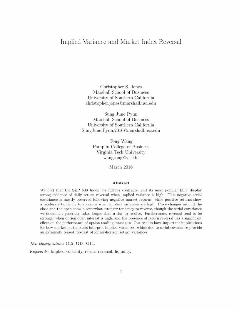
Figure 2 shows averages of monthly values of total autocovariance constructed from these daily
returns, where monthly total autocovariances are defined as in (5). Values on the left side of the
graph show results based on prices sampled some number of minutes before the close. Values on the
right show results from prices sampled after the open. The value obtained from end-of-day prices,
used elsewhere in the paper, is highlighted, as is the value calculated based on prices observed one
minute after the open.
The figure shows that daily returns based on prices just following the open have a much more
negative amount of serial covariance, suggesting that order imbalances near the open may be large.
The serial covariance of returns based on closing prices is smaller, but still somewhat more negative
than covariances based on prices away from the open and close. Thus, there is perhaps modest
evidence that prices around the close show a greater tendency to revert relative to prices sampled
closer to the middle of the trading day.
We next reexamine our main finding, that return reversal strengthens with implied variance,
using the same timing alternatives. Figure 3 therefore shows the slope coefficients of monthly
regressions of total autocovariances on lagged implied variances, which are computed based on the
15

VIX index, where only the timing of the daily price series is changed.
In short, there is only modest evidence that returns based on end-of-day prices behave much
differently. Although the slope coefficient is maximized just prior to the close, the value of that
coefficient is not very different to coefficients obtained at different times of the day. What is perhaps
more notable is that the reversal of returns constructed based on prices just following the open is
not particularly strong when implied variances are high, even though reversal of those prices is high
unconditionally.
3.2 Timing of returns around the close
From Table 5, we know that a substantial amount of serial covariance is beyond the first order,
implying that reversal requires horizons of several days or more to complete. Nevertheless, there
remains the possibility that part of the return reversal we have seen happens over a much shorter
time frame. We investigate this by analyzing the relation between returns in the last N minutes of
one day and the return from the close of that day to N minutes following the next day’s open.
We perform this investigation by analyzing the performance of a reversal-based trading strategy.
This strategy will buy futures following negative returns and sell futures following positive returns.
The size of the position will be increasing in the magnitude of these returns. In addition, to make
strategies with different holding periods more comparable we will hold larger positions when the
holding period is shorter.
These goals are achieved using the following weight:
−0.01× rate of return in last N minutes of day t
E [|return in last N minutes of the day|] E [|return from close to N minutes after next open|]The interpretation of the numerator is natural – we short futures following positive returns and
go long following negative returns, with position sizes that are proportional to the return. The
denominator is chosen so that the expected absolute portfolio return, or
E [|weight× return from close of day t to N minutes after t+ 1 open|]
is equal to 0.01 on average, at least approximately.
Implementation of this strategy requires estimates of the two expectations in the denominator.
16

Since these are estimates of absolute values, they should be estimated with reasonable accuracy
even in small samples. We therefore proxy for each expectation using the average of the most recent
22 lagged values.
Figure 4 shows the average return, in basis points per day, on this strategy as a function of N .
The result is a clear peak in average returns roughly between N = 20 and N = 60. To be more
specific, the figure shows that a trader who bought or sold at the close based on the return over the
prior 30 minutes, and then held that position until 30 minutes after the next open, would earn on
average slightly more than 12 basis points per day. This is a significant return given the moderate
volatility of the strategy.7
Figure 5 shows how the expected return on the same trading strategies vary with implied
variance. The values plotted are simply the slope coefficients obtained from regressing trading
strategy returns on the lagged implied variance, which is again computed based on the VIX. Since
negative serial correlation will imply positive returns on a reversal strategy, we expect these slope
coefficients to be positive based on what we have seen so far. The figure shows that they are indeed
generally positive, and that the profitability of very short term reversal strategies, particularly
those with N between 5 and 45, are the most positive.
To summarize, in this section we have seen that although reversal is apparent at a daily horizon
or longer, there is a tendency for reversal to be particularly stronger over a much smaller window
before the market close and after the subsequent open. Reversal in this time frame is stronger
unconditionally, but it is particularly strong when implied variance is high.
3.3 Option open interest and return reversal
Given the somewhat special nature of return reversal right around the close, we hypothesize that
there may be tendency for order imbalances to concentrate towards the end of the day. While there
are many reasons why this might be the case, one possibility is that derivatives traders make their
final hedge-rebalancing trades at that time before markets close for the night.
7The strategy is designed to have an expected absolute return of 1% per day. If returns were normally distributed,
then their standard deviation would be slightly higher, around 1.25%. In our data, returns are not normal and the
standard deviations are closer to 2%.
17

Besides giving a reason for why end-of-day reversal is particularly strong, an explanation based
on derivatives hedging could also give a rationale for the importance of implied variance in driving
return reversal. Specifically, higher implied variance is clearly a strong proxy for greater risk, which
makes hedging derivatives positions more critical. In addition, Jones (2003) shows that variance
and market returns become more highly correlated when variances rise. Thus, in times of high
variance, traders are not only able to delta-hedge using index futures, but they can also partially
hedge their ‘vega’ risk as well.
If derivatives hedging is indeed a factor behind return reversal, then we would expect reversal
strength to depend on the size of the option positions being hedged. Without a perfect proxy for
the extent of these positions, we rely simply on the open interest in the S&P 500 Index options
market, measured as the total number of puts and calls. Since open interest has trended upward as
option markets have increased in prominence, we also consider a detrended version of open interest
that is calculated by subtracting the lagged 66-day moving average of open interest from the current
value.
Because open interest can change quickly, often due to option expiration, we find that open
interest is primarily useful in predicting serial covariances over horizons of less than a month.
Table 7 reports the results of weekly regressions in which the dependent variable is the total
autocovariance from each week. This is computed similarly to (5) except that it uses all the returns
in a week rather than in a month. The independent variables include the implied variance and the
option open interest, both from the last day of the previous week (typically Friday). Regression
also include an interaction term.
In regressions by itself, we see that open interest has a negative but insignificant effect on return
autocovariance. When we include implied variance as a second predictor, the negative coefficient on
open interest becomes significant in the two specifications that use detrended open interest. When
we add an interaction term involving both implied variance and open interest, we find significance
in all four regressions.
Overall, the regression evidence suggests a modest but significant role for options markets.
Greater open interest means that any increase in implied variance is more likely to predict future
18

return reversals. This is consistent with the hypothesis that trades related to option hedging become
larger or more impatient when market uncertainty is high.
4 Reversal-based trading strategies in S&P 500 Index options
In theory, option prices should be unaffected by serial correlation. That statement, made most
clearly by Lo and Wang (1995), reflects the fact that serial covariance is a property of the conditional
mean of returns. Since option prices are determined under the equivalent martingale measure,
where all conditional means are equal to the riskless rate, there is no role for serial covariance in
the valuation of options. That said, serial covariance can affect the payoff of an option, and thus it
could be an important determinant of expected option returns. This is the issue we investigate in
this section.
As a motivating example, imagine an options trader who has purchased both an at-the-money
call and an at-the-money put, both with two days until expiration. This position, the so-called
‘straddle,’ is often interpreted as being a bet on the volatility of the underlying asset, since its
payoff is sensitive only to the magnitude and not the direction of price movements.
Now suppose, one day later, that the underlying security’s price has declined substantially. This
is good news for the option trader, who sees a high likelihood of a large payoff from the put option
that is now in the money. However, if the returns on the underlying asset exhibit a tendency to
reverse, then large profits may not materialize, as the underlying will tend to revert back towards
its starting value, where the option payoffs may be too small to cover the cost of the straddle.
Thus, negative autocovariance will tend to reduce the payoffs of positions, like straddles and
options in general, that are positive bets on volatility. But since negative autocovariance does not
affect the price of those positions, those lower payoffs will have the effect of reducing expected option
returns. Thus, strategies like the straddle will exhibit poor performance when serial covariance is
negative.
There is a way for the trader to avoid the harm due to serial covariance, however. Following
the same substantial decline in the underlying security’s price, the trader could protect themselves
by selling the straddle that they purchased originally and replacing it with a new at-the-money
19

(ATM) straddle.
By doing so the trader accomplishes two things. First, the trader locks in the gains that have
resulted from owning a put option that is now in the money.8 Second, by rebalancing into a new
ATM straddle, the option trader eliminates all directional dependence in his or her portfolio. So
whether or not the subsequent day sees a reversal, the option trader is indifferent.
In this section we examine the performance of zero delta ATM straddles. These combine the
put and call that, for a given maturity, are closest to being at the money, The call and put are not
held in exactly the same quantity, but are rather weighted so that the Black-Scholes delta of the
combined portfolio is exactly zero. This helps ensure that the strategy represents a pure bet on
volatility rather than on the direction of the S&P 500 Index.
We compare the strategy of buying an ATM straddle and holding it for many days to the
alternative of buying an ATM straddle and then rolling it over into a new ATM straddle at the end
of each trading day. We refer to these two strategies as ‘buy-and-hold’ and ‘daily rebalanced.’ We
examine their average returns, alphas, and betas, and how all three depend on the level of implied
variance.
We analyze option trading strategies on a monthly basis. We initiate new ATM straddle posi-
tions on the day that regular options expire, namely the third Friday of the month. Buy-and-hold
strategies involving straddles with two or three months remaining until expiration are held until
expiration Friday of the next month. Because of well known issues involving noise in option prices
close to expiration, the buy-and-hold strategy for the one-month straddle holds the position for one
week less, exiting the trade on the Friday prior to expiration week. Daily rebalanced strategies are
invested over the same time periods, but instead of holding the position fixed they are rebalanced
into a new zero-delta ATM straddle at the end of each day. We assume that all transactions take
place at the bid-ask midpoint.
Table 8 shows results for the returns on the buy-and-hold and rebalanced strategies. In addition,
8One might imagine that this put option would be relatively cheap even though it is in the money, given that mean
reversion will tend to reduce the value of the put’s payoff at expiration. However, as discussed above, the valuation
of this option is unaffected by serial covariance, so the expected shrinkage in the final payoff does not have any effect
on the option’s price.
20

we examine the differences between those returns, where the buy-and-hold return is subtracted from
the rebalanced return. While results vary slightly by maturity, a number of patterns are apparent.
First, average returns on buy-and-hold strategies are lower than average returns on rebalanced
strategies. These are reported in the table as intercept-only regressions. While the difference
between those means is not statistically significant, it is consistent with the unconditionally neg-
ative autocovariance we find in our sample, which has a more detrimental effect on buy-and-hold
performance.
When we regress buy-and-hold returns on lagged implied variance, we find a negative coefficient,
again consistent with more negative serial correlation worsening performance, but again it is not
significant. However, when we look at the difference between the rebalanced and buy-and-hold
strategies, we find that return differences are significantly related to the level of implied variance.
This is due to the fact that while buy-and-hold and rebalanced returns are strongly correlated, only
the former has its performance adversely impacted by negative serial correlation. This result holds
for all three option tenors.
If we add the excess market returns to the regression, by themselves and interacted with lagged
implied variance, then we can interpret the parameters as describing time-varying alphas and
betas. In these regressions, the alphas on the buy-and-hold strategies are decreasing in implied
variance, while the alphas on the rebalanced strategies are increasing. The alphas of the return
differences (or the differences between the alphas) are increasing and statistically significant. Both
beta parameters are statistically insignificant for the return differences due to the fact that the
betas of the buy-and-hold and rebalanced strategies largely cancel out.
5 Conclusion
In this paper we demonstrate a simple but surprising fact, namely that higher levels of implied
variance are associated with negative serial covariance in the returns on the S&P 500 Index, its
futures contracts, and its most popular ETF. This finding suggests that even the most liquid equity-
linked assets may in some situations display return reversal. It also confirms the finding of Nagel
(2012) that the VIX is a significant predictor of market illiquidity.
21

One implication of our findings is that implied volatilities may provide an extremely biased
view of market risk for an investor with an investment horizon of a month or more. When implied
variances rise, fully a half if not more of that increase represents a purely transient component,
which affects daily returns but that washes out completely by a one-month horizon.
Although we find substantial evidence of return reversal at horizons longer than one day, return
reversal appears to be particularly strong around the daily close and the daily open, suggesting a
concentration of order imbalances at those points. Furthermore, the reversal in very short-term
returns right around the daily close is most sensitive to changes in implied variance, suggesting
that order imbalances at the close are increasing in times of market uncertainty. We investigate the
possibility that reversal is related to trades by option hedgers, which might be expected to cluster
at the close, by examining the role of open interest in return reversal. We find strong evidence that
open interest in S&P 500 Index options strengthens the negative serial covariance in index returns.
Finally, we examine the effects that serial covariance has on the performance of option trading
strategies. We find that buy-and-hold strategies involving zero delta straddles perform badly rela-
tive to strategies that rebalance daily into new zero-delta straddles when implied variances are high.
We argue that this is due to the fact that by maintaining their zero delta, the rebalanced strat-
egy effectively immunizes the options trader from negative autocorrelation, which would otherwise
cause his expected option payoffs to be diminished.
A somewhat unexpected finding was that return reversal was mainly if not solely present fol-
lowing negative returns. Positive returns showed a tendency, though it was not as significant, to
continue rather than reverse. Understanding why this continuation exists and how it is manifested
at different return horizons is ongoing work.
22

References
Ahn, Dong-Hyun, Jacob Boudoukh, Matthew Richardson, and Robert F. Whitelaw (2002), “Partial
adjustment or stale prices? Implications from stock index and futures return autocorrelations.”
Review of Financial Studies, 15, 655–689.
Andersen, Torben G. and Tim Bollerslev (1998), “Answering the skeptics: Yes, standard volatility
models do provide accurate forecasts.” International Economic Review, 885–905.
Avramov, Doron, Tarun Chordia, and Amit Goyal (2006), “Liquidity and autocorrelations in indi-
vidual stock returns.” Journal of Finance, 61, 2365–2394.
Barberis, Nicholas (2000), “Investing for the long run when returns are predictable.” Journal of
Finance, 55, 225–264.
Bates, David S. (2012), “U.S. stock market crash risk, 1926–2010.” Journal of Financial Economics,
105, 229–259.
Ben-Rephael, Azi, Shmuel Kandel, and Avi Wohl (2011), “The price pressure of aggregate mutual
fund flows.” Journal of Financial and Quantitative Analysis, 46, 585–603.
Blair, Bevan J., Ser-Huang Poon, and Stephen J. Taylor (2001), “Forecasting S&P 100 volatility:
The incremental information content of implied volatilities and high-frequency index returns.”
Journal of Econometrics, 105, 5–26.
Bollerslev, Tim, Viktor Todorov, and Lai Xu (2015), “Tail risk premia and return predictability.”
Journal of Financial Economics, 118, 113–134.
Britten-Jones, Mark and Anthony Neuberger (2000), “Option prices, implied price processes, and
stochastic volatility.” Journal of Finance, 55, 839–866.
Campbell, John Y., Sanford J. Grossman, and Jiang Wang (1993), “Trading volume and serial
correlation in stock returns.” Quarterly Journal of Economics, 108, 905–939.
23

Campbell, John Y. and Luis M. Viceira (2002), Strategic asset allocation: Portfolio choice for
long-term investors. Oxford University Press, USA.
Canina, Linda and Stephen Figlewski (1993), “The informational content of implied volatility.”
Review of Financial Studies, 6, 659–681.
Chernov, Mikhail (2007), “On the role of risk premia in volatility forecasting.” Journal of Business
& Economic Statistics, 25, 411–426.
Chordia, Tarun, Richard Roll, and Avanidhar Subrahmanyam (2002), “Order imbalance, liquidity,
and market returns.” Journal of Financial Economics, 65, 111–130.
Christensen, Bent J. and Nagpurnanand R. Prabhala (1998), “The relation between implied and
realized volatility.” Journal of Financial Economics, 50, 125–150.
Collin-Dufresne, Pierre and Kent Daniel (2015), “Liquidity and return reversals.” Working paper.
Conrad, Jennifer and Gautam Kaul (1988), “Time-variation in expected returns.” Journal of Busi-
ness, 409–425.
Da, Zhi, Qianqiu Liu, and Ernst Schaumburg (2014), “A closer look at the short-term return
reversal.” Management Science, 60, 658–674.
Day, Theodore E. and Craig M. Lewis (1992), “Stock market volatility and the information content
of stock index options.” Journal of Econometrics, 52, 267–287.
Etula, Erkko, Kalle Rinne, Matti Suominen, and Lauri Vaittinen (2015), “Dash for cash: Month-
end liquidity needs and the predictability of stock returns.” Working paper.
Fisher, Lawrence (1966), “Some new stock-market indexes.” Journal of Business, 39, 191–225.
French, Kenneth R., G. William Schwert, and Robert F. Stambaugh (1987), “Expected stock
returns and volatility.” Journal of Financial Economics, 19, 3–29.
Jones, Christopher S. (2003), “The dynamics of stochastic volatility: Evidence from underlying
and options markets.” Journal of Econometrics, 116, 181–224.
24

Khandani, Amir E. and Andrew W. Lo (2007), “What happened to the quants in August 2007?”
Journal of Investment Management, 5, 29–78.
Lamoureux, Christopher G. and William D. Lastrapes (1993), “Forecasting stock-return variance:
Toward an understanding of stochastic implied volatilities.” Review of Financial Studies, 6, 293–
326.
LeBaron, Blake (1992), “Some relations between volatility and serial correlations in stock market
returns.” Journal of Business, 199–219.
Lehmann, Bruce N. (1990), “Fads, martingales, and market efficiency.” Quarterly Journal of Eco-
nomics, 1–28.
Lo, Andrew W. and A. Craig MacKinlay (1988), “Stock market prices do not follow random walks:
Evidence from a simple specification test.” Review of Financial Studies, 1, 41–66.
Lo, Andrew W. and A. Craig MacKinlay (1990), “When are contrarian profits due to stock market
overreaction?” Review of Financial Studies, 3, 175–205.
Lo, Andrew W. and Jiang Wang (1995), “Implementing option pricing models when asset returns
are predictable.” Journal of Finance, 50, 87–129.
Merton, Robert C. (1980), “On estimating the expected return on the market: An exploratory
investigation.” Journal of Financial Economics, 8, 323–361.
Nagel, Stefan (2012), “Evaporating liquidity.” Review of Financial Studies, 25, 2005–2039.
Poterba, James M. and Lawrence H. Summers (1988), “Mean reversion in stock prices: Evidence
and implications.” Journal of Financial Economics, 22, 27–59.
25

Figure 1: Annualized volatility predictions based on monthly and daily variance regressions. This
figure plots the conditional volatilities implied by regressions (1) and (2), estimated using S&P 500
Index futures returns, as a function of the VIX index.
26
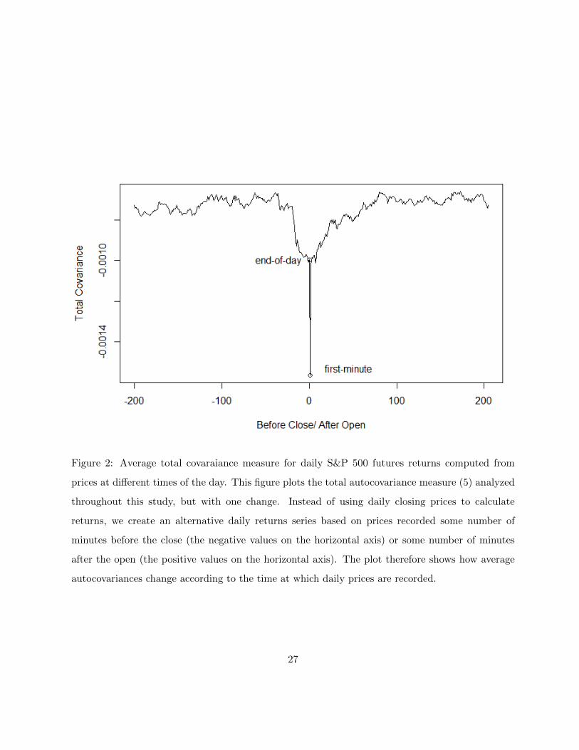
Figure 2: Average total covaraiance measure for daily S&P 500 futures returns computed from
prices at different times of the day. This figure plots the total autocovariance measure (5) analyzed
throughout this study, but with one change. Instead of using daily closing prices to calculate
returns, we create an alternative daily returns series based on prices recorded some number of
minutes before the close (the negative values on the horizontal axis) or some number of minutes
after the open (the positive values on the horizontal axis). The plot therefore shows how average
autocovariances change according to the time at which daily prices are recorded.
27

Figure 3: Implied variance slope coefficient from regressions of total covaraiance measure for daily
S&P 500 futures returns computed from prices at different times of the day. This figure plots the
slope coefficients resulting from regressing the total autocovariance measure (5) analyzed through-
out this study on lagged implied variance. The only difference with other results is that daily
returns are based on prices recorded some number of minutes before the close (the negative values
on the horizontal axis) or some number of minutes after the open (the postive values on the hori-
zontal axis), rather than only on closing prices. The plot therefore shows how the responsiveness of
autocovariance to implied variance changes according to the time at which daily prices are recorded.
28

Figure 4: Average return for reversal-based S&P 500 futures strategies with different formation and
holding period lengths. In this graph we plot average returns, in basis points per day, of strategies
formed on the basis of the return in the last N minutes of one day, where the trade is initiated at
that day’s close and held until N minutes following the next day’s open. The horizontal axis of the
figure represents N . The strategy involves putting the following weight, at the close of day t, in
the front-month futures contract:
−0.01× rate of return in last N minutes of day t
E [|return in last N minutes of the day|] E [|return from close to N minutes after next open|]We proxy for the two expected values using averages over the 22 days leading up to day t−1. A
portfolio with this weight holds a position that is negatively related to the return in the last N
minutes of the formation day. Furthermore, this portfolio should have a return, regardless of the
investment horizon, whose expected absolute value is approximately 0.01.
29

Figure 5: Implied variance slope coefficient from regressions of returns on reversal-based S&P 500
futures strategies with different formation and holding period lengths. Following Figure 4, we
consider reversal based strategies formed on the basis of the return in the last N minutes of one
day, where the trade is initiated at that day’s close and held until N minutes following the next
day’s open. The portfolio weight is designed so that the portfolio return has an expected absolute
value of approximately 0.01 regardless of N . The figure shows the results of regressing strategy
returns on lagged implied variance for different values of N , which is represented on the horizontal
axis.
30

Table 1
# ofobs. Mean SD AC(1) Mean SD AC(1) Mean T-stat SD AC(1)
S&P 500 Index 311 0.0027 0.0048 0.7145 0.0018 0.0033 0.2070 -0.0008 -4.2824 0.0036 0.32761/1990-11/2015
S&P 500 Futures 311 0.0028 0.0053 0.6294 0.0018 0.0034 0.2044 -0.0010 -4.5752 0.0038 0.35041/1990-11/2015
SPY ETF 274 0.0030 0.0055 0.6300 0.0018 0.0032 0.2223 -0.0011 -4.9156 0.0040 0.36502/1993-11/2015
Mean SD AC(1)
0.0038 0.0037 0.84961/1990-11/2015
This table reports summary statistics for our two variance proxies and for the VIX index. Data are monthly. Variance proxies are based on continuously
compounded returns, where returns on the S&P 500 Index and the SPY ETF are in excess of the riskless rate. Returns are not demeaned. The difference is
computed as the monthly squared return minus the sum of daily squared returns. Statistics reported are the mean, standard deviation, and first-order
autocorrelation. We also report t-statistics for the difference between the two variance proxies, which are based on Newey-West standard errors with five
lags. Sample periods are determined by data availability.
Monthly squared returnsSum of squared daily returns Difference
Squared rescaled VIX
31

Table 2
Asset/Sample IVol Intercept Slope R2 Intercept Slope R2
S&P 500 Index VIX -0.0008 0.9254 0.4395 0.0003 0.4078 0.18242/1990-11/2015 (-1.9590) (5.5512) (1.2996) (8.1619)
S&P 500 Futures VIX -0.0008 0.9522 0.3821 0.0003 0.4083 0.17392/1990-11/2015 (-1.7729) (5.3430) (1.3021) (7.9686)
SPY ETF VIX -0.0007 0.9517 0.4445 0.0003 0.3908 0.09952/1993-11/2015 (-1.7235) (5.4911) (1.3932) (7.6212)
S&P 500 Futures VIX 0.0000 0.7004 0.6648 0.0005 0.3855 0.37922/1990-12/2002 (-0.1056) (8.6478) (1.9324) (6.3658)
S&P 500 Futures VIX -0.0009 1.0437 0.3840 0.0001 0.4179 0.22951/2003-11/2015 (-2.5208) (5.1406) (0.4417) (6.1135)
S&P 500 Futures VXO 0.0001 0.7610 0.0887 0.0006 0.3455 0.10532/1986-11/2015 (0.1523) (4.0257) (2.3605) (8.2957)
Squared monthly returnsSum of squared daily returns
This table reports monthly regressions of different realized variance proxies on lagged one-month implied variances, which are calculated
based on the VIX or VXO indexes. Variance proxies are based on continuously compounded returns, where returns on the S&P 500 Index
and the SPY ETF are in excess of the riskless rate. Returns are not demeaned. T-statistics, in parentheses, are computed using the Newey-
West procedure with eight lags. Sample periods are determined by data availability.
32

Table 3
Asset/Sample IVol Intercept Slope R2
S&P 500 Index VIX 0.0011 -0.5170 0.23822/1990-11/2015 (1.9829) (-2.8754)
S&P 500 Futures VIX 0.0011 -0.5439 0.23482/1990-11/2015 (1.9007) (-2.9085)
SPY ETF VIX 0.0010 -0.5609 0.24912/1993-11/2015 (1.8627) (-2.9688)
S&P 500 Futures VIX 0.0005 -0.3150 0.08112/1990-12/2002 (2.5012) (-5.7549)
S&P 500 Futures VIX 0.0011 -0.6258 0.31071/2003-11/2015 (1.9069) (-2.9545)
S&P 500 Futures VXO 0.0004 -0.4155 0.05192/1986-11/2015 (0.5470) (-2.3568)
Total autocovariance
This table reports monthly regressions of the total autocovariance measure, which
is defined as the monthly squared return minus the sum of squared daily returns,
where returns on the S&P 500 Index and the SPY ETF are in excess of the riskless
rate. The independent variable is a lagged one-month implied variance, calculated
based on either the VIX or VXO index. T-statistics, in parentheses, are computed
using the Newey-West procedure with eight lags. Sample periods are determined
by data availability.
33

Table 4
Intercept R2
0.0051 -0.0388 0.0000(1.1964) (-0.0279)
0.0043 0.0119 0.0000(0.4425) (0.0609)
0.0068 -0.0001 0.0002(0.5839) (-0.1901)
Intercept R2
0.0076 -0.5674 0.0026(2.3055) (-0.5946)
0.0089 -0.0616 0.0011(1.1449) (-0.4068)
0.0044 0.0000 0.0000(0.4509) (0.1007)
This table reports regressions of monthly continuously compounded futures
returns on various transformations of the lagged one-month implied variance
(IV ), which is calculated based on either the VIX or VXO index. T-statistics, in
parentheses, are computed using the Newey-West procedure with five lags.
Sample periods are determined by data availability.
IV based on the VIX index, 2/1990-11/2015
IV based on the VXO index, 2/1986-11/2015
𝐼𝑉𝐼𝑉 1/ 𝐼𝑉
𝐼𝑉𝐼𝑉 1/ 𝐼𝑉
34

Table 5
Asset/Sample IVol Intercept Slope R2 Intercept Slope R2
S&P 500 Index VIX 0.0005 -0.1954 0.1248 0.0006 -0.3233 0.13592/1990-11/2015 (3.4699) (-4.0154) (1.2270) (-2.2007)
S&P 500 Futures VIX 0.0004 -0.1756 0.1136 0.0007 -0.3699 0.15412/1990-11/2015 (3.5685) (-4.3658) (1.3190) (-2.3582)
SPY ETF VIX 0.0003 -0.1768 0.1240 0.0007 -0.3850 0.15742/1993-11/2015 (3.1890) (-5.6994) (1.2366) (-2.1953)
S&P 500 Futures VIX 0.0003 -0.0959 0.0374 0.0002 -0.2240 0.03952/1990-12/2002 (1.5361) (-1.6258) (1.0993) (-2.9892)
S&P 500 Futures VIX 0.0003 -0.2028 0.1499 0.0008 -0.4230 0.23971/2003-11/2015 (1.9470) (-5.7033) (1.3365) (-2.2466)
S&P 500 Futures VXO 0.0003 -0.1441 0.1060 0.0001 -0.2718 0.02262/1986-11/2015 (2.5787) (-3.3866) (0.1762) (-1.9373)
This table reports monthly regressions of first order and higher order autocovariance measures on on lagged one-month implied
variance, calculated based on either the VIX or VXO index. The two autocovariance measured are based on the decomposition
where the first term can be interpreted as a first-order autocovariance while the second term includes all higher orders. T-statistics,
in parentheses, are computed using the Newey-West procedure with eight lags. Sample periods are determined by data availability.
1st order autocovariance Higher order autocovariance
35

Table 6
Asset/Sample IVol Intercept Slope R2 Intercept Slope R2
S&P 500 Index VIX -0.0005 0.2218 0.0234 0.0016 -0.7405 0.16092/1990-11/2015 (-1.7106) (2.8574) (2.4335) (-4.2676)
S&P 500 Futures VIX -0.0005 0.1910 0.0174 0.0016 -0.7365 0.15352/1990-11/2015 (-1.9027) (2.6352) (2.2898) (-3.9002)
SPY ETF VIX -0.0006 0.2374 0.0271 0.0017 -0.7992 0.18062/1993-11/2015 (-1.9688) (3.2846) (2.2549) (-4.0173)
S&P 500 Futures VIX -0.0006 0.1911 0.0098 0.0012 -0.5110 0.04972/1990-12/2002 (-1.2382) (1.4327) (1.9293) (-3.4734)
S&P 500 Futures VIX -0.0004 0.1899 0.0243 0.0015 -0.8157 0.23141/2003-11/2015 (-1.1755) (2.1507) (1.8439) (-3.8150)
S&P 500 Futures VXO 0.0001 0.0138 0.0056 -0.0009 -0.0471 0.01722/1986-11/2015 (0.4867) (2.3515) (-3.0114) (-1.3714)
This table reports monthly regressions of asymmetric autocovariance proxies on on lagged one-month implied variance, calculated based on
either the VIX or VXO index. on the squared and rescaled VIX or VXO index. Asymmetric autocovariances are computed based on the
decomposition
where the two terms differ because one term includes all pairs of returns in which the first return is positive, while the other term includes
pairs in which the first return is negative. T-statistics, in parentheses, are computed using the Newey-West procedure with eight lags.
Sample periods are determined by data availability.
First return is positive First return is negative
36
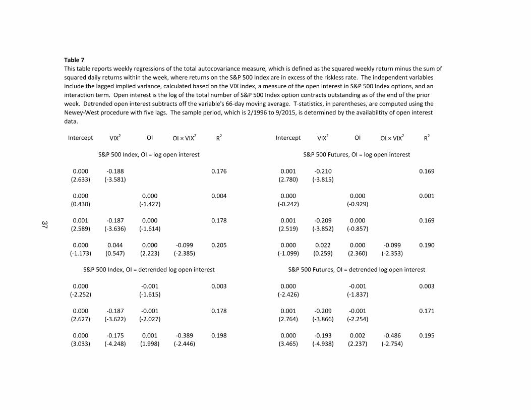
Table 7
Intercept VIX2 OI OI × VIX2R2 Intercept VIX2 OI OI × VIX2
R2
0.000 -0.188 0.176 0.001 -0.210 0.169(2.633) (-3.581) (2.780) (-3.815)
0.000 0.000 0.004 0.000 0.000 0.001(0.430) (-1.427) (-0.242) (-0.929)
0.001 -0.187 0.000 0.178 0.001 -0.209 0.000 0.169(2.589) (-3.636) (-1.614) (2.519) (-3.852) (-0.857)
0.000 0.044 0.000 -0.099 0.205 0.000 0.022 0.000 -0.099 0.190(-1.173) (0.547) (2.223) (-2.385) (-1.099) (0.259) (2.360) (-2.353)
0.000 -0.001 0.003 0.000 -0.001 0.003(-2.252) (-1.615) (-2.426) (-1.837)
0.000 -0.187 -0.001 0.178 0.001 -0.209 -0.001 0.171(2.627) (-3.622) (-2.027) (2.764) (-3.866) (-2.254)
0.000 -0.175 0.001 -0.389 0.198 0.000 -0.193 0.002 -0.486 0.195(3.033) (-4.248) (1.998) (-2.446) (3.465) (-4.938) (2.237) (-2.754)
S&P 500 Index, OI = detrended log open interest S&P 500 Futures, OI = detrended log open interest
This table reports weekly regressions of the total autocovariance measure, which is defined as the squared weekly return minus the sum of
squared daily returns within the week, where returns on the S&P 500 Index are in excess of the riskless rate. The independent variables
include the lagged implied variance, calculated based on the VIX index, a measure of the open interest in S&P 500 Index options, and an
interaction term. Open interest is the log of the total number of S&P 500 Index option contracts outstanding as of the end of the prior
week. Detrended open interest subtracts off the variable's 66-day moving average. T-statistics, in parentheses, are computed using the
Newey-West procedure with five lags. The sample period, which is 2/1996 to 9/2015, is determined by the availabiltity of open interest
data.
S&P 500 Index, OI = log open interest S&P 500 Futures, OI = log open interest
37
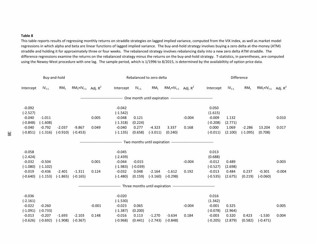
Table 8
Intercept IVt-1 RMt RMt×IVt-1 Adj. R2 Intercept IVt-1 RMt RMt×IVt-1 Adj. R2 Intercept IVt-1 RMt RMt×IVt-1 Adj. R2
-0.092 -0.042 0.050(-2.527) (-1.542) (1.615)-0.040 -1.011 0.005 -0.048 0.121 -0.004 -0.009 1.132 0.010
(-0.848) (-1.608) (-1.318) (0.224) (-0.208) (2.771)-0.040 -0.792 -2.037 -9.867 0.049 -0.040 0.277 -4.323 3.337 0.168 0.000 1.069 -2.286 13.204 0.017
(-0.851) (-1.316) (-0.910) (-0.453) (-1.135) (0.658) (-3.011) (0.240) (-0.011) (2.100) (-1.095) (0.708)
-0.058 -0.045 0.013(-2.424) (-2.439) (0.688)-0.032 -0.504 0.001 -0.044 -0.015 -0.004 -0.012 0.489 0.003
(-1.080) (-1.102) (-1.983) (-0.039) (-0.527) (2.698)-0.019 -0.436 -2.401 -1.311 0.124 -0.032 0.048 -2.164 -1.612 0.192 -0.013 0.484 0.237 -0.301 -0.004
(-0.640) (-1.153) (-1.865) (-0.165) (-1.480) (0.159) (-3.160) (-0.298) (-0.535) (2.675) (0.219) (-0.060)
-0.036 -0.020 0.016(-2.161) (-1.530) (1.342)-0.022 -0.260 -0.001 -0.023 0.065 -0.004 -0.001 0.325 0.005
(-1.091) (-0.733) (-1.387) (0.200) (-0.078) (2.964)-0.013 -0.207 -1.693 -2.103 0.148 -0.016 0.113 -1.270 -3.634 0.184 -0.003 0.320 0.423 -1.530 0.004
(-0.626) (-0.692) (-1.908) (-0.367) (-0.968) (0.441) (-2.743) (-0.848) (-0.205) (2.879) (0.582) (-0.471)
----------------------------------- Two months until expiration -----------------------------------
----------------------------------- Three months until expiration -----------------------------------
This table reports results of regressing monthly returns on straddle strategies on lagged implied variance, computed from the VIX index, as well as market model
regressions in which alpha and beta are linear functions of lagged implied variance. The buy-and-hold strategy involves buying a zero delta at-the-money (ATM)
straddle and holding it for approximately three or four weeks. The rebalanced strategy involves rebalancing daily into a new zero delta ATM straddle. The
difference regressions examine the returns on the rebalanced strategy minus the returns on the buy-and-hold strategy. T-statistics, in parentheses, are computed
using the Newey-West procedure with one lag. The sample period, which is 1/1996 to 8/2015, is determined by the availabiltity of option price data.
Buy-and-hold Rebalanced to zero delta Difference
----------------------------------- One month until expiration -----------------------------------
38
Top Related