


Languages
Pages
Legal


Image Enhancement in
Spatial Domain
UNIT-2
P. Balamurugan, Assistant Professor
PG & Research Department of Computer Science
Government Arts College, Coimbatore -641018
Email: [email protected]
Digital Image Processing 2
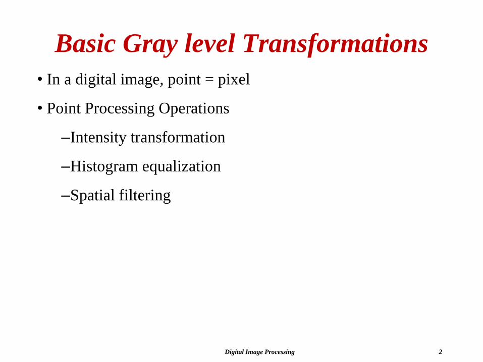
Basic Gray level Transformations
• In a digital image, point = pixel
• Point Processing Operations
–Intensity transformation
–Histogram equalization
–Spatial filtering

Digital Image Processing 3
Intensity Transformation Functions
• s=T(r) , where r denotes the
intensity of f and s is the intensity
of g, both at any (x, y) in the
image
• imadjust
– g=imadjust(f,[low_in high_in],
[low_out high_out], gamma)
– Values between low_in and
high_in is mapped to values
between low_out and high_out
low_inhigh_in
low_out
high_out
gamma<1
low_inhigh_in
low_out
high_out
gamma>1
Digital Image Processing 4
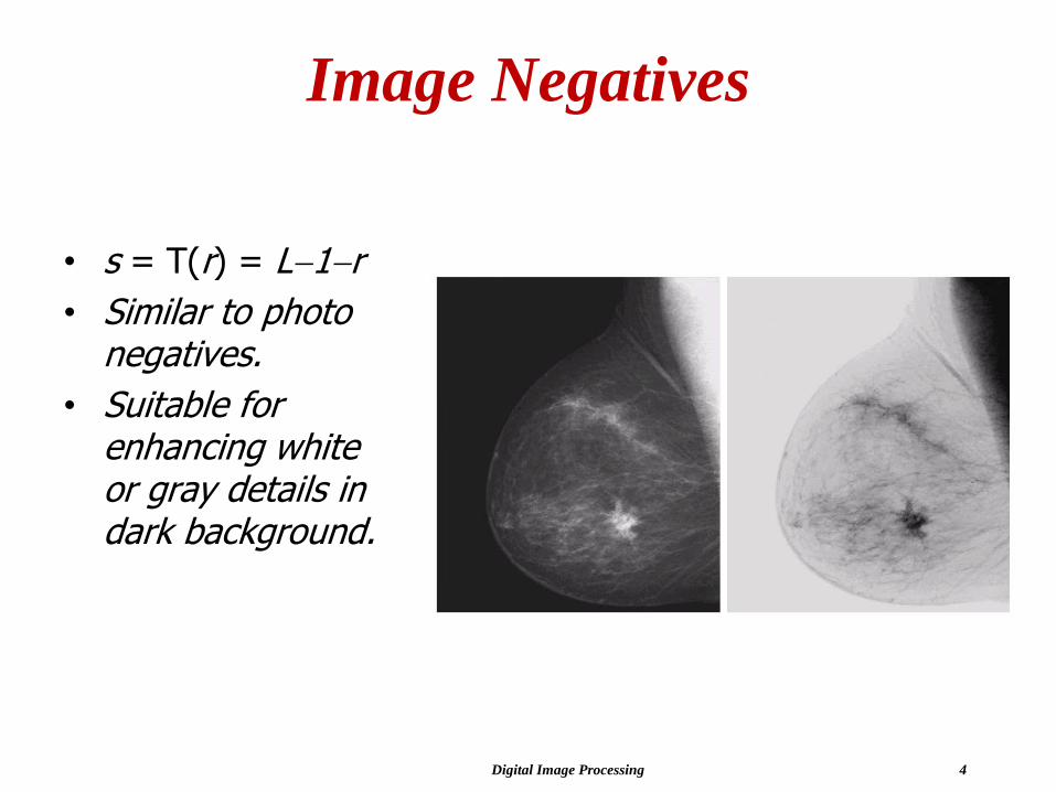
Image Negatives
• s = T(r) = L-1-r
• Similar to photo negatives.
• Suitable for enhancing white or gray details in dark background.

Digital Image Processing 5
Power Law Gray-level Transform
• Gamma correction: to compensate the built-in power law compression due to display characteristics.
s = T(r) = crg
Digital Image Processing 6
Contrast Enhancement• Piecewise linear Transformation
• Input : Poor illumination images
• Lack of dynamic range
• Increase the dynamic range of gray levels
• In raw imagery, data occupies only a small portion of the
available range of digital values (commonly 8 bits or 256
levels).
• Contrast enhancement involves changing the original values
so that more of the available range is used,
• Increases the contrast between targets and their backgrounds.
Digital Image Processing 7
Other Piece-wise Transformation
Gray level Slicing
Bit plane slice
Digital Image Processing 8
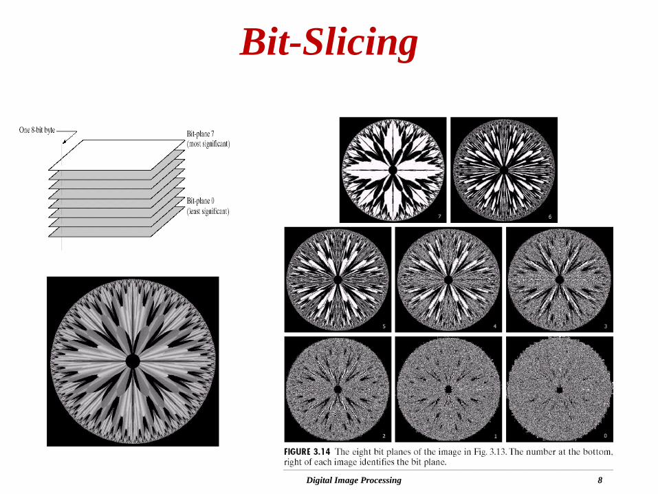
Bit-Slicing
Digital Image Processing 9
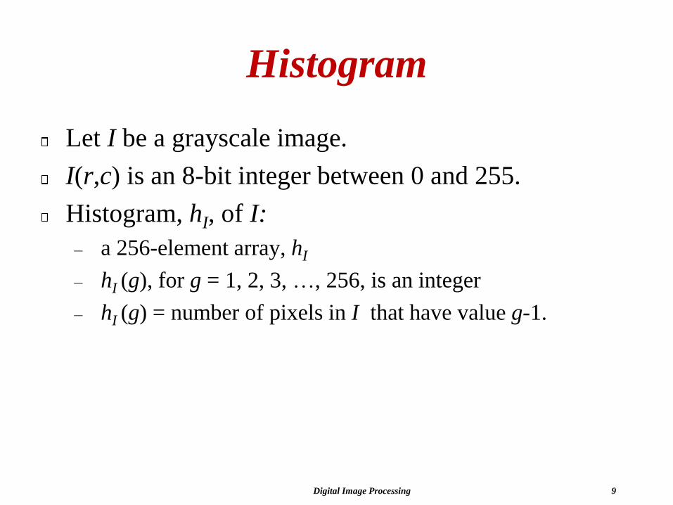
Histogram
Let I be a grayscale image.
I(r,c) is an 8-bit integer between 0 and 255.
Histogram, hI, of I:
– a 256-element array, hI
– hI (g), for g = 1, 2, 3, …, 256, is an integer
– hI (g) = number of pixels in I that have value g-1.
Digital Image Processing 10
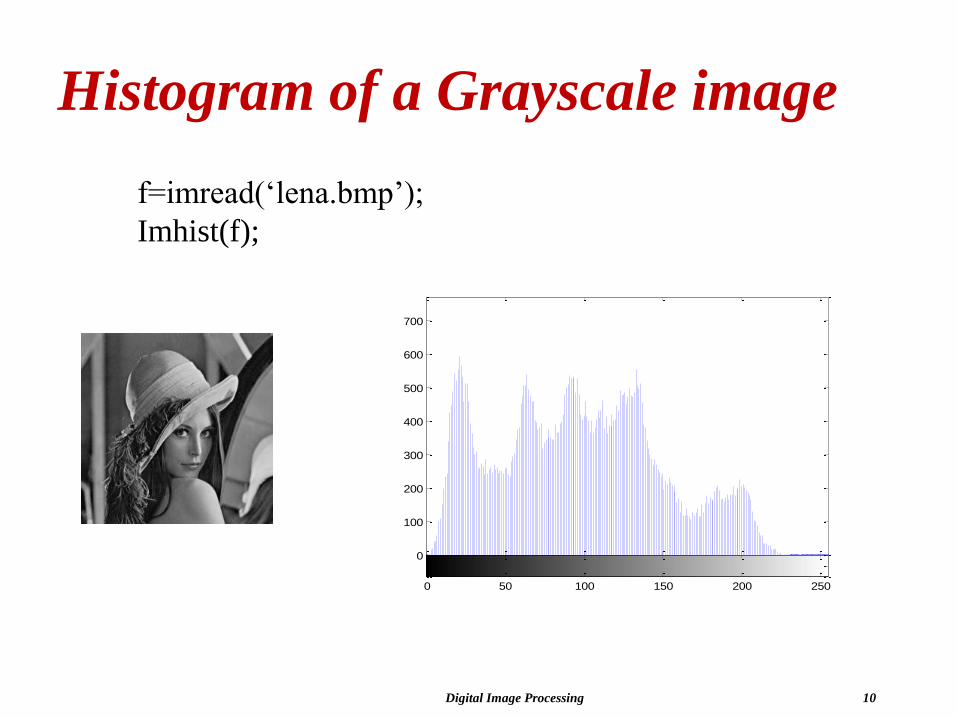
Histogram of a Grayscale image
0
100
200
300
400
500
600
700
0 50 100 150 200 250
f=imread(‘lena.bmp’);
Imhist(f);
Digital Image Processing 11
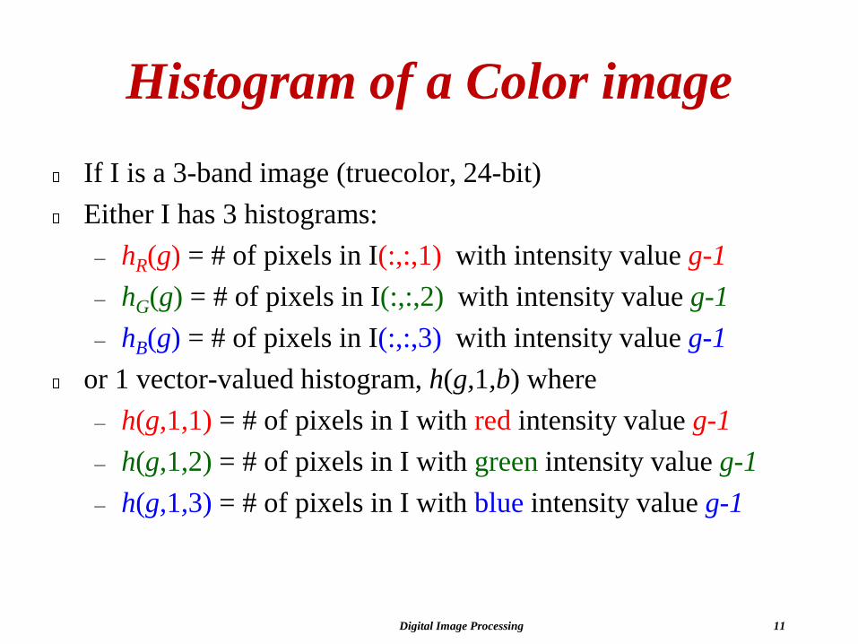
Histogram of a Color image
If I is a 3-band image (truecolor, 24-bit)
Either I has 3 histograms:
– hR(g) = # of pixels in I(:,:,1) with intensity value g-1
– hG(g) = # of pixels in I(:,:,2) with intensity value g-1
– hB(g) = # of pixels in I(:,:,3) with intensity value g-1
or 1 vector-valued histogram, h(g,1,b) where
– h(g,1,1) = # of pixels in I with red intensity value g-1
– h(g,1,2) = # of pixels in I with green intensity value g-1
– h(g,1,3) = # of pixels in I with blue intensity value g-1
Digital Image Processing 12
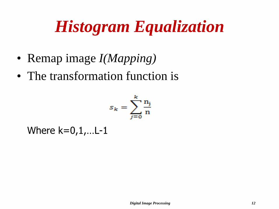
Histogram Equalization
• Remap image I(Mapping)
• The transformation function is
Where k=0,1,…L-1
Digital Image Processing 13
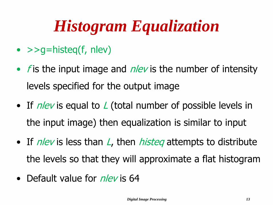
Histogram Equalization
• >>g=histeq(f, nlev)
• f is the input image and nlev is the number of intensity
levels specified for the output image
• If nlev is equal to L (total number of possible levels in
the input image) then equalization is similar to input
• If nlev is less than L, then histeq attempts to distribute
the levels so that they will approximate a flat histogram
• Default value for nlev is 64
Digital Image Processing 14
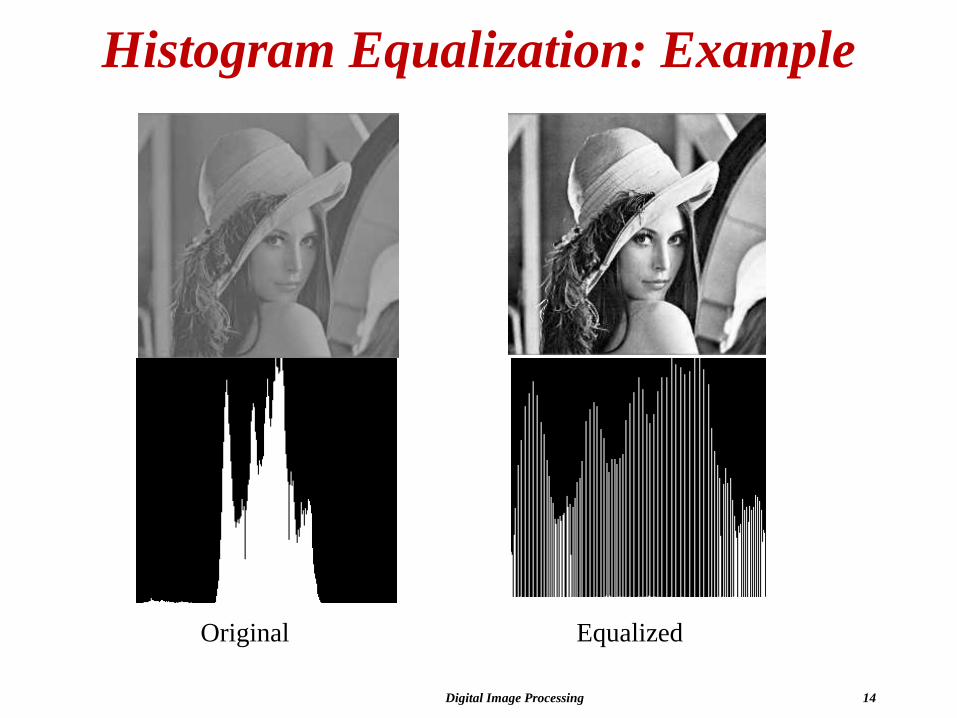
Histogram Equalization: Example
Original Equalized
Digital Image Processing 15
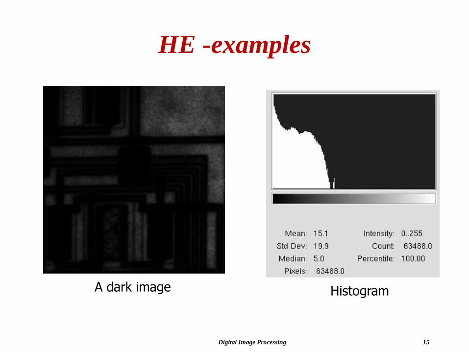
HE -examples
A dark image Histogram
Digital Image Processing 16
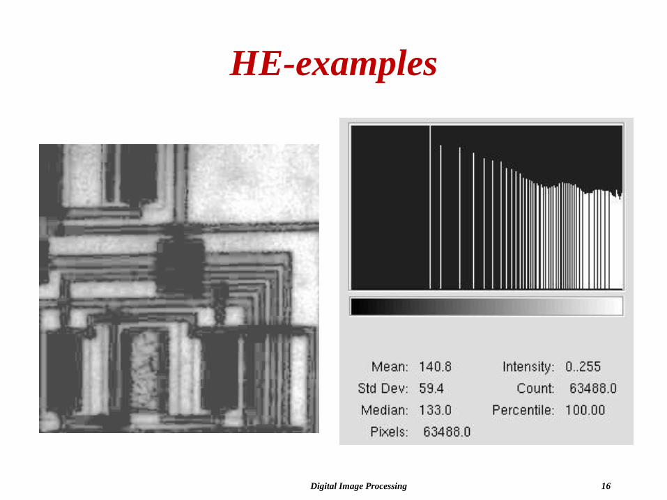
HE-examples

Digital Image Processing 17
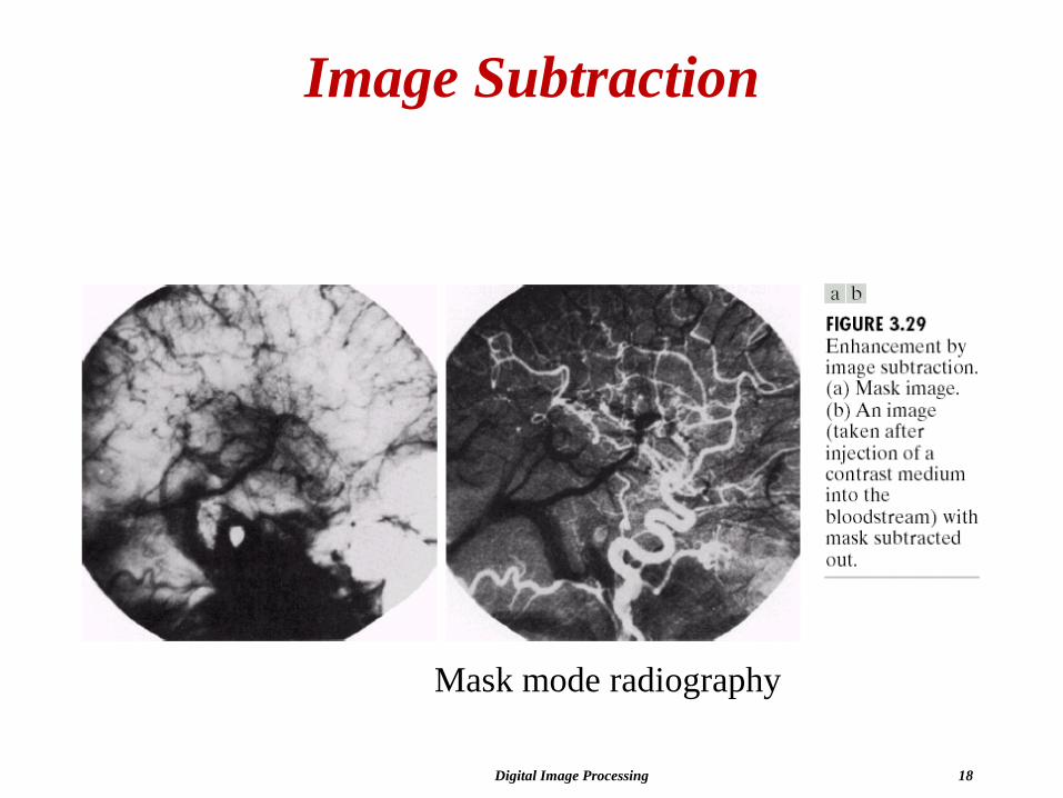
Image Subtraction
• A more interesting arithmetic operation is pixel-wise subtraction of two images.
• Refer to the fractal image again.),(),(),( yxhyxfyxg -=
difference
4 lower-order bit planes zeroed out
original
contrast enhanced
Digital Image Processing 18
Image Subtraction
Mask mode radiography
Digital Image Processing 19
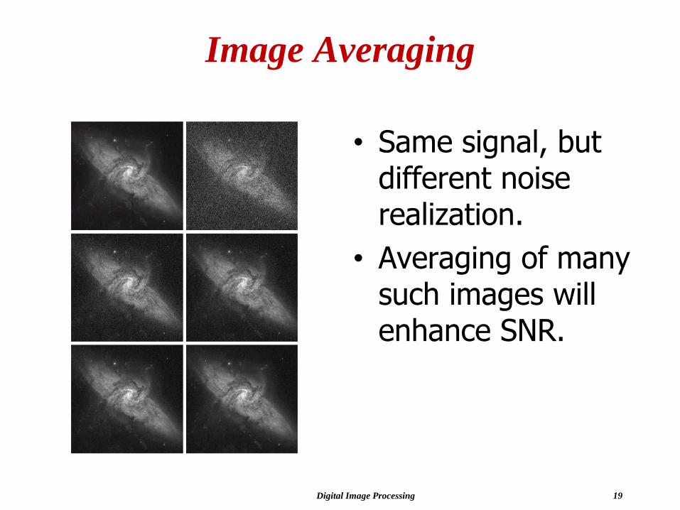
Image Averaging
• Same signal, but different noise realization.
• Averaging of many such images will enhance SNR.
Digital Image Processing 20
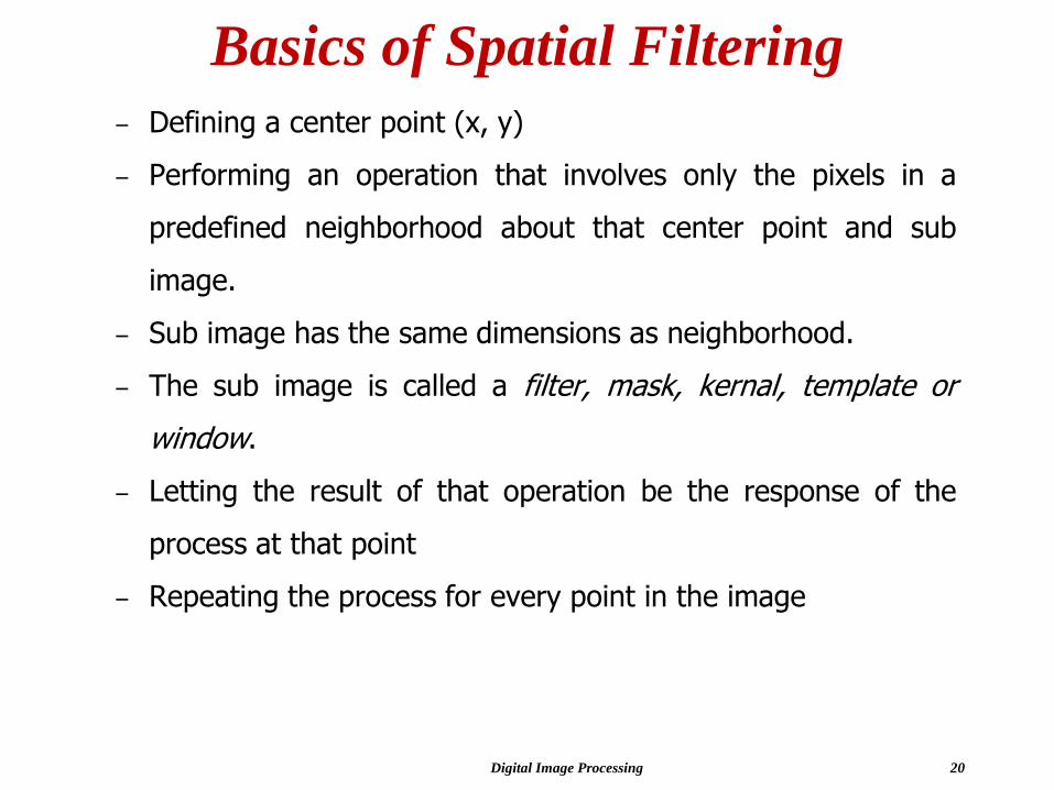
Basics of Spatial Filtering
– Defining a center point (x, y)
– Performing an operation that involves only the pixels in a
predefined neighborhood about that center point and sub
image.
– Sub image has the same dimensions as neighborhood.
– The sub image is called a filter, mask, kernal, template or
window.
– Letting the result of that operation be the response of the
process at that point
– Repeating the process for every point in the image

Digital Image Processing 21
Process of Spatial Filtering
The process consists of,
– Moving the filter mask from point to point in an image.
– At each point (x, y), the response of the filter at that point is
calculated.
– The response is sum of products of the filter coefficients and
the corresponding image pixels in the area spanned by the
filter mask.
– It is similar to frequency domain concept called convolution.
– So, the linear filtering process is often referred to as
“Convolving a mask with an image”

Digital Image Processing 22
New pixel = v*e + z*a + y*b +x*c + w*d
+ u*e + t*f + s*g + r*h
r s t
u v w
x y z
Kernel
a b c
d e e
f g h
Source
Pixels

Digital Image Processing 23
Convolution➢ Response R of an m × n mask at any point (x, y), is
expressed as follows:
➢ Example : For the 3 × 3 general mask, the response atany point (x,y) in the image is given by,

Digital Image Processing 24
Correlation and Convolution
• Correlation is the process of passing themask w by the image array f
• Convolution is the same process, except thatw is rotated by 1800 prior to passing it by f
0 0 0 1 0 0 0 0 1 2 3 2 0
0 0 0 1 0 0 0 0 0 2 3 2 1
f wCorrelation
Convolution
Digital Image Processing 25
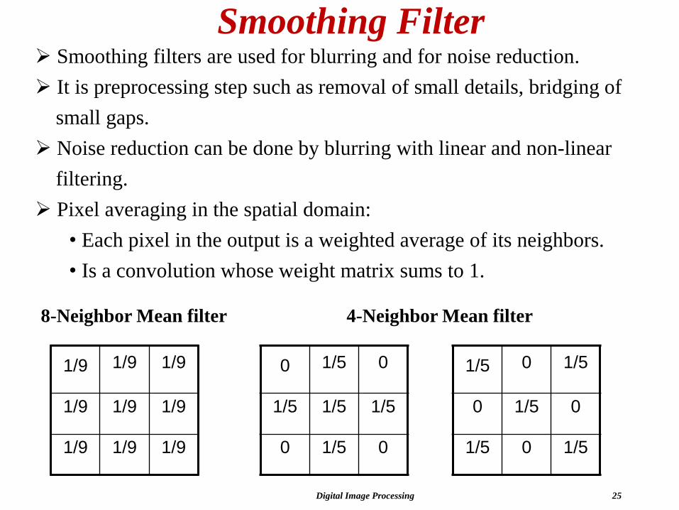
Smoothing Filter➢ Smoothing filters are used for blurring and for noise reduction.
➢ It is preprocessing step such as removal of small details, bridging of
small gaps.
➢ Noise reduction can be done by blurring with linear and non-linear
filtering.
➢ Pixel averaging in the spatial domain:
• Each pixel in the output is a weighted average of its neighbors.
• Is a convolution whose weight matrix sums to 1.
1/9 1/9 1/9
1/9 1/9 1/9
1/9 1/9 1/9
0 1/5 0
1/5 1/5 1/5
0 1/5 0
1/5 0 1/5
0 1/5 0
1/5 0 1/5
8-Neighbor Mean filter 4-Neighbor Mean filter

Digital Image Processing 26
Smoothing Filter
➢ These filters are also called averaging filter/low-pass filter.
➢ Idea behind Smoothing filters are straightforward.
➢ i.e. Replacing the value of every pixel in an image by the average
of the gray levels in the neighborhood defined by the filter mask.
➢ The result is reduced “sharp” transitions in gray levels.
➢ Order statistics filter- Mean, median
➢ Reduces Salt & pepper noise
1 1 1
1 1 1
1 1 1
1 2 1
2 4 2
1 2 1
1/9 ×
Digital Image Processing 27
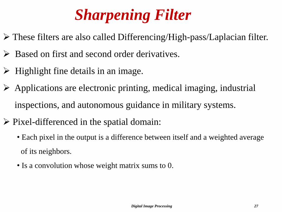
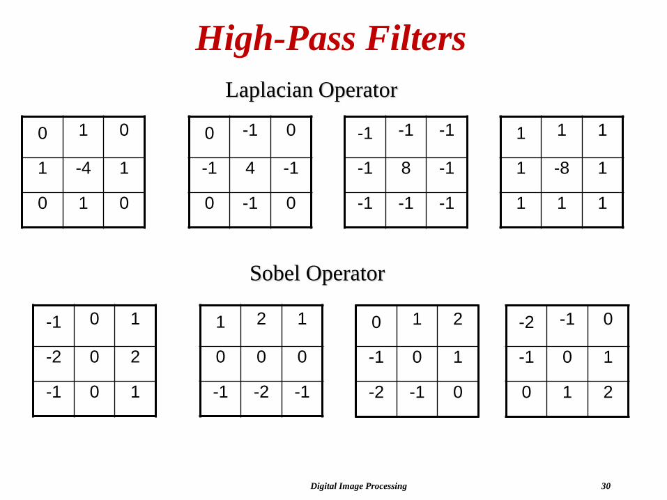
Sharpening Filter
➢ These filters are also called Differencing/High-pass/Laplacian filter.
➢ Based on first and second order derivatives.
➢ Highlight fine details in an image.
➢ Applications are electronic printing, medical imaging, industrial
inspections, and autonomous guidance in military systems.
➢ Pixel-differenced in the spatial domain:
• Each pixel in the output is a difference between itself and a weighted average
of its neighbors.
• Is a convolution whose weight matrix sums to 0.

Digital Image Processing 28
Blurring vs. Sharpening➢ Blurring/smooth is done in spatial domain by pixel averaging in a
neighbors, it is a process of integration.
➢ Sharpening is an inverse process, to find the difference by the
neighborhood, done by spatial differentiation.
Digital Image Processing 29
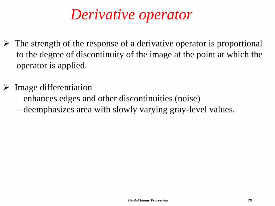
Derivative operator
➢ The strength of the response of a derivative operator is proportional
to the degree of discontinuity of the image at the point at which the
operator is applied.
➢ Image differentiation
– enhances edges and other discontinuities (noise)
– deemphasizes area with slowly varying gray-level values.
Digital Image Processing 30
0 -1 0
-1 4 -1
0 -1 0
0 1 0
1 -4 1
0 1 0
-1 -1 -1
-1 8 -1
-1 -1 -1
1 1 1
1 -8 1
1 1 1
1 2 1
0 0 0
-1 -2 -1
-1 0 1
-2 0 2
-1 0 1
-2 -1 0
-1 0 1
0 1 2
0 1 2
-1 0 1
-2 -1 0
High-Pass Filters
Laplacian Operator
Sobel Operator
Digital Image Processing 31
References➢ https://www.slideshare.net/CristinaPrezBenito/simultaneous-
smoothing-and-sharpening-of-color-images.
➢ https://www.javatpoint.com/digital-image-processing-tutorial.
➢ https://www.tutorialspoint.com/dip/index.html.
TEXT BOOKS
1) Rafael C. Gonzalez, Richard E. Woods, “Digital Image Processing”, Second
Edition, PHI/Pearson Education.
2) Alexander M., Abid K., “OpenCV-Python Tutorials”, 2017.
REFERENCE BOOKS
1) B. Chanda, D. Dutta Majumder, “Digital Image Processing and Analysis”, PHI,
2003.
2) Nick Efford, “Digital Image Processing a practical introducing using Java”,
Pearson Education, 2004.
Top Related