


![Automatic - microsoft.com...system is computationally more exp ensiv e. 2 Linear class of face geometries W e the same represen tation for the face mo dels as in [8]. A face is represen](https://static.fdocuments.in/doc/165x107/5f3dc7f42217a912f4022a78/automatic-system-is-computationally-more-exp-ensiv-e-2-linear-class-of-face.jpg)


Languages
Pages
Legal

IEEE Trans. on PAMI, July 1997.
Eigenfaces vs. Fisherfaces:
Recognition Using Class Speci�c Linear Projection
Peter N. Belhumeur Jo~ao P. Hespanha David J. Kriegman
Center for Computational Vision and Control
Dept. of Electrical Engineering
Yale University
New Haven, CT 06520-8267
Phone: 203-432-4249
Fax: 203-432-7481
Abstract
We develop a face recognition algorithm which is insensitive to gross variation in
lighting direction and facial expression. Taking a pattern classi�cation approach,
we consider each pixel in an image as a coordinate in a high-dimensional space. We
take advantage of the observation that the images of a particular face, under varying
illumination but �xed pose, lie in a 3-D linear subspace of the high dimensional
image space { if the face is a Lambertian surface without shadowing. However,
since faces are not truly Lambertian surfaces and do indeed produce self-shadowing,
images will deviate from this linear subspace. Rather than explicitly modeling
this deviation, we linearly project the image into a subspace in a manner which
discounts those regions of the face with large deviation. Our projection method is
based on Fisher's Linear Discriminant and produces well separated classes in a low-
dimensional subspace even under severe variation in lighting and facial expressions.
The Eigenface technique, another method based on linearly projecting the image
space to a low dimensional subspace, has similar computational requirements. Yet,
extensive experimental results demonstrate that the proposed \Fisherface" method
has error rates that are lower than those of the Eigenface technique for tests on the
Harvard and Yale Face Databases.

Index Terms: Appearance-Based Vision, Face Recognition, Illumination Invariance,
Fisher's Linear Discriminant

Figure 1. The same person seen under di�erent lighting conditions can appear dramaticallydi�erent: In the left image, the dominant light source is nearly head-on; in the right image, thedominant light source is from above and to the right.
1 Introduction
Within the last several years, numerous algorithms have been proposed for face recogni-
tion; for detailed surveys see [1, 2]. While much progress has been made toward recogniz-
ing faces under small variations in lighting, facial expression and pose, reliable techniques
for recognition under more extreme variations have proven elusive.
In this paper we outline a new approach for face recognition { one that is insensitive
to large variations in lighting and facial expressions. Note that lighting variability in-
cludes not only intensity, but also direction and number of light sources. As is evident
from Figure 1, the same person, with the same facial expression and seen from the same
viewpoint, can appear dramatically di�erent when light sources illuminate the face from
di�erent directions. See also Figure 4.
Our approach to face recognition exploits two observations:
1. All of the images of a Lambertian surface, taken from a �xed viewpoint but under
varying illumination, lie in a 3-D linear subspace of the high-dimensional image
space [3].

2. Because of regions of shadowing, specularities, and facial expressions, the above
observation does not exactly hold. In practice, certain regions of the face may have
variability from image to image that often deviates signi�cantly from the linear
subspace and, consequently, are less reliable for recognition.
We make use of these observations by �nding a linear projection of the faces from the
high-dimensional image space to a signi�cantly lower dimensional feature space which
is insensitive both to variation in lighting direction and facial expression. We choose
projection directions that are nearly orthogonal to the within-class scatter, projecting
away variations in lighting and facial expression while maintaining discriminability. Our
method Fisherfaces, a derivative of Fisher's Linear Discriminant (FLD) [4, 5], maximizes
the ratio of between-class scatter to that of within-class scatter.
The Eigenface method is also based on linearly projecting the image space to a low
dimensional feature space [6, 7, 8]. However, the Eigenface method, which uses principal
components analysis (PCA) for dimensionality reduction, yields projection directions that
maximize the total scatter across all classes, i.e. across all images of all faces. In choosing
the projection which maximizes total scatter, PCA retains unwanted variations due to
lighting and facial expression. As illustrated in Figures 1 and 4 and stated by Moses, Adini,
and Ullman, \the variations between the images of the same face due to illumination and
viewing direction are almost always larger than image variations due to change in face
identity" [9]. Thus, while the PCA projections are optimal for reconstruction from a low
dimensional basis, they may not be optimal from a discrimination standpoint.
We should point out that Fisher's Linear Discriminant is a \classical" technique in
pattern recognition [4], �rst developed by Robert Fisher in 1936 for taxonomic classi�ca-
tion [5]. Depending upon the features being used, it has been applied in di�erent ways
in computer vision and even in face recognition. Cheng et al. presented a method that

used Fisher's discriminator for face recognition where features were obtained by a polar
quantization of the shape [10]. Baker and Nayar have developed a theory of pattern re-
jection which is based on a two class linear discriminant [11]. Contemporaneous with
our work [12], Cui, Swets, and Weng applied Fisher's discriminator (using di�erent termi-
nology, they call it the Most Discriminating Feature { MDF) in a method for recognizing
hand gestures [13]. Though no implementation is reported, they also suggest that the
method can be applied to face recognition under variable illumination.
In the sections to follow, we compare four methods for face recognition under variation
in lighting and facial expression: correlation, a variant of the linear subspace method
suggested by [3], the Eigenface method [6, 7, 8], and the Fisherface method developed
here. The comparisons are done using both a subset of the Harvard Database (330
images) [14, 15] and a database created at Yale (176 images). In tests on both databases,
the Fisherface method had lower error rates than any of the other three methods. Yet,
no claim is made about the relative performance of these algorithms on much larger
databases.
We should also point out that we have made no attempt to deal with variation in
pose. An appearance-based method such as ours can be extended to handle limited pose
variation using either a multiple-view representation such as Pentland, Moghaddam, and
Starner's View-based Eigenspace [16] or Murase and Nayar's Appearance Manifolds [17].
Other approaches to face recognition that accommodate pose variation include [18, 19, 20].
Furthermore, we assume that the face has been located and aligned within the image, as
there are numerous methods for �nding faces in scenes [21, 22, 20, 23, 24, 25, 7].

2 Methods
The problem can be simply stated: Given a set of face images labeled with the person's
identity (the learning set) and an unlabeled set of face images from the same group of
people (the test set), identify each person in the test images.
In this section, we examine four pattern classi�cation techniques for solving the face
recognition problem, comparing methods that have become quite popular in the face
recognition literature, namely correlation [26] and Eigenface methods [6, 7, 8], with alter-
native methods developed by the authors. We approach this problem within the pattern
classi�cation paradigm, considering each of the pixel values in a sample image as a coor-
dinate in a high-dimensional space (the image space).
2.1 Correlation
Perhaps, the simplest classi�cation scheme is a nearest neighbor classi�er in the image
space [26]. Under this scheme, an image in the test set is recognized (classi�ed) by
assigning to it the label of the closest point in the learning set, where distances are
measured in the image space. If all of the images are normalized to have zero mean and
unit variance, then this procedure is equivalent to choosing the image in the learning set
that best correlates with the test image. Because of the normalization process, the result
is independent of light source intensity and the e�ects of a video camera's automatic gain
control.
This procedure, which subsequently is referred to as correlation, has several well-known
disadvantages. First, if the images in the learning set and test set are gathered under
varying lighting conditions, then the corresponding points in the image space may not
be tightly clustered. So in order for this method to work reliably under variations in
lighting, we would need a learning set which densely sampled the continuum of possible
lighting conditions. Second, correlation is computationally expensive. For recognition,
we must correlate the image of the test face with each image in the learning set; in
an e�ort to reduce the computation time, implementors [27] of the algorithm described
in [26] developed special purpose VLSI hardware. Third, it requires large amounts of
storage { the learning set must contain numerous images of each person.
2.2 Eigenfaces
As correlation methods are computationally expensive and require great amounts of stor-
age, it is natural to pursue dimensionality reduction schemes. A technique now commonly
used for dimensionality reduction in computer vision { particularly in face recognition {
is principal components analysis (PCA) [14, 17, 6, 7, 8]. PCA techniques, also known as
Karhunen-Loeve methods, choose a dimensionality reducing linear projection that maxi-
mizes the scatter of all projected samples.
More formally, let us consider a set of N sample images fx1;x2; : : : ;xNg taking values
in an n-dimensional image space, and assume that each image belongs to one of c classes
fX1; X2; : : : ; Xcg. Let us also consider a linear transformation mapping the original n-
dimensional image space into an m-dimensional feature space, where m < n. The new
feature vectors yk 2 IRm are de�ned by the following linear transformation:
yk = W Txk k = 1; 2; : : : ; N (1)
where W 2 IRn�m is a matrix with orthonormal columns.
If the total scatter matrix ST is de�ned as
ST =
NX
k=1
(xk � �)(xk � �)T
where c is the number of classes and � 2 IRn is the mean image of all samples, then after
applying the linear transformation W T , the scatter of the transformed feature vectors

fy1;y2; : : : ;yNg is W TSTW . In PCA, the projection Wopt is chosen to maximize the
determinant of the total scatter matrix of the projected samples, i.e.
Wopt = argmaxW
jW TSTW j (2)
=�w1 w2 : : : wm
�
where fwi j i = 1; 2; : : : ; mg is the set of n-dimensional eigenvectors of ST corresponding
to the m largest eigenvalues. Since these eigenvectors have the same dimension as the
original images, they are referred to as Eigenpictures in [6] and Eigenfaces in [7, 8]. If
classi�cation is performed using a nearest neighbor classi�er in the reduced feature space
and m is chosen to be the number of images N in the training set, then the Eigenface
method is equivalent to the correlation method in the previous section.
A drawback of this approach is that the scatter being maximized is due not only to the
between-class scatter that is useful for classi�cation, but also to the within-class scatter
that, for classi�cation purposes, is unwanted information. Recall the comment by Moses,
Adini and Ullman [9]: Much of the variation from one image to the next is due to illumi-
nation changes. Thus if PCA is presented with images of faces under varying illumination,
the projection matrix Wopt will contain principal components (i.e. Eigenfaces) which re-
tain, in the projected feature space, the variation due lighting. Consequently, the points
in the projected space will not be well clustered, and worse, the classes may be smeared
together.
It has been suggested that by discarding the three most signi�cant principal compo-
nents, the variation due to lighting is reduced. The hope is that if the �rst principal
components capture the variation due to lighting, then better clustering of projected
samples is achieved by ignoring them. Yet it is unlikely that the �rst several principal
components correspond solely to variation in lighting; as a consequence, information that
is useful for discrimination may be lost.

2.3 Linear Subspaces
Both correlation and the Eigenface method are expected to su�er under variation in
lighting direction. Neither method exploits the observation that for a Lambertian surface
without shadowing, the images of a particular face lie in a 3-D linear subspace.
Consider a point p on a Lambertian surface illuminated by a point light source at
in�nity. Let s 2 IR3 be a column vector signifying the product of the light source intensity
with the unit vector for the light source direction. When the surface is viewed by a camera,
the resulting image intensity of the point p is given by
E(p) = a(p)n(p)T s (3)
where n(p) is the unit inward normal vector to the surface at the point p, and a(p) is the
albedo of the surface at p [28]. This shows that the image intensity of the point p is linear
on s 2 IR3. Therefore, in the absence of shadowing, given three images of a Lambertian
surface from the same viewpoint taken under three known, linearly independent light
source directions, the albedo and surface normal can be recovered; this is the well known
method of photometric stereo [29, 30]. Alternatively, one can reconstruct the image of the
surface under an arbitrary lighting direction by a linear combination of the three original
images, see [3].
For classi�cation, this fact has great importance: it shows that for a �xed viewpoint,
the images of a Lambertian surface lie in a 3-D linear subspace of the high-dimensional
image space. This observation suggests a simple classi�cation algorithm to recognize
Lambertian surfaces { insensitive to a wide range of lighting conditions.
For each face, use three or more images taken under di�erent lighting directions to con-
struct a 3-D basis for the linear subspace. Note that the three basis vectors have the same
dimensionality as the training images and can be thought of as basis images. To perform
recognition, we simply compute the distance of a new image to each linear subspace and

choose the face corresponding to the shortest distance. We call this recognition scheme
the Linear Subspace method. We should point out that this method is a variant of the
photometric alignment method proposed in [3], and is a special case of the more elaborate
recognition method described in [15]. Subsequently, Nayar and Murase have exploited the
apparent linearity of lighting to augment their appearance manifold [31].
If there is no noise or shadowing, the Linear Subspace algorithmwould achieve error free
classi�cation under any lighting conditions, provided the surfaces obey the Lambertian
re ectance model. Nevertheless, there are several compelling reasons to look elsewhere.
First, due to self-shadowing, specularities, and facial expressions, some regions in images
of the face have variability that does not agree with the linear subspace model. Given
enough images of faces, we should be able to learn which regions are good for recognition
and which regions are not. Second, to recognize a test image we must measure the distance
to the linear subspace for each person. While this is an improvement over a correlation
scheme that needs a large number of images to represent the variability of each class, it
is computationally expensive. Finally, from a storage standpoint, the Linear Subspace
algorithm must keep three images in memory for every person.
2.4 Fisherfaces
The previous algorithm takes advantage of the fact that under admittedly idealized con-
ditions, the variation within class lies in a linear subspace of the image space. Hence,
the classes are convex and therefore linearly separable. One can perform dimensionality
reduction using linear projection and still preserve linear separability. This is a strong
argument in favor of using linear methods for dimensionality reduction in the face recog-
nition problem, at least when one seeks insensitivity to lighting conditions.
Since the learning set is labeled, it makes sense to use this information to build a more
reliable method for reducing the dimensionality of the feature space. Here we argue that
class 1class 2
0
0
feature 1
feat
ure
2
PCA
FLD
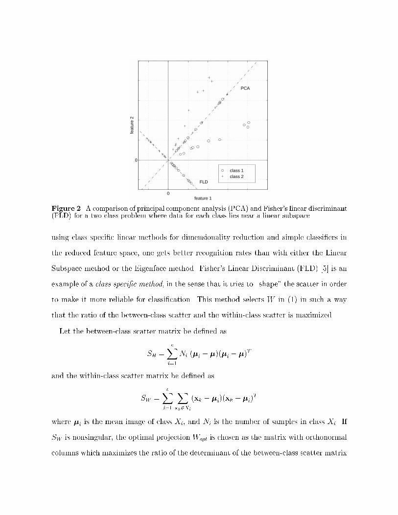
Figure 2. A comparison of principal component analysis (PCA) and Fisher's linear discriminant(FLD) for a two class problem where data for each class lies near a linear subspace.
using class speci�c linear methods for dimensionality reduction and simple classi�ers in
the reduced feature space, one gets better recognition rates than with either the Linear
Subspace method or the Eigenface method. Fisher's Linear Discriminant (FLD) [5] is an
example of a class speci�c method, in the sense that it tries to \shape" the scatter in order
to make it more reliable for classi�cation. This method selects W in (1) in such a way
that the ratio of the between-class scatter and the within-class scatter is maximized.
Let the between-class scatter matrix be de�ned as
SB =
cX
i=1
Ni (�i � �)(�i � �)T
and the within-class scatter matrix be de�ned as
SW =
cX
i=1
X
xk2Xi
(xk � �i)(xk � �i)T
where �i is the mean image of class Xi, and Ni is the number of samples in class Xi. If
SW is nonsingular, the optimal projection Wopt is chosen as the matrix with orthonormal
columns which maximizes the ratio of the determinant of the between-class scatter matrix
of the projected samples to the determinant of the within-class scatter matrix of the
projected samples, i.e.
Wopt = argmaxW
jW TSBW j
jW TSWW j(4)
=�w1 w2 : : : wm
�
where fwi j i = 1; 2; : : : ; mg is the set of generalized eigenvectors of SB and SW corre-
sponding to the m largest generalized eigenvalues f�i j i = 1; 2; : : : ; mg, i.e.
SBwi = �iSWwi ; i = 1; 2; : : : ; m:
Note that there are at most c�1 nonzero generalized eigenvalues, and so an upper bound
on m is c� 1 where c is the number of classes. See [4].
To illustrate the bene�ts of class speci�c linear projection, we constructed a low dimen-
sional analogue to the classi�cation problem in which the samples from each class lie near
a linear subspace. Figure 2 is a comparison of PCA and FLD for a two-class problem in
which the samples from each class are randomly perturbed in a direction perpendicular to
a linear subspace. For this example N = 20, n = 2, and m = 1. So the samples from each
class lie near a line passing through the origin in the 2-D feature space. Both PCA and
FLD have been used to project the points from 2-D down to 1-D. Comparing the two pro-
jections in the �gure, PCA actually smears the classes together so that they are no longer
linearly separable in the projected space. It is clear that although PCA achieves larger
total scatter, FLD achieves greater between-class scatter, and consequently classi�cation
becomes easier.
In the face recognition problem one is confronted with the di�culty that the within-
class scatter matrix SW 2 IRn�n is always singular. This stems from the fact that the
rank of SW is at most N � c, and in general, the number of images in the learning set N
is much smaller than the number of pixels in each image n. This means that it is possible
to choose the matrix W such that the within-class scatter of the projected samples can
be made exactly zero.
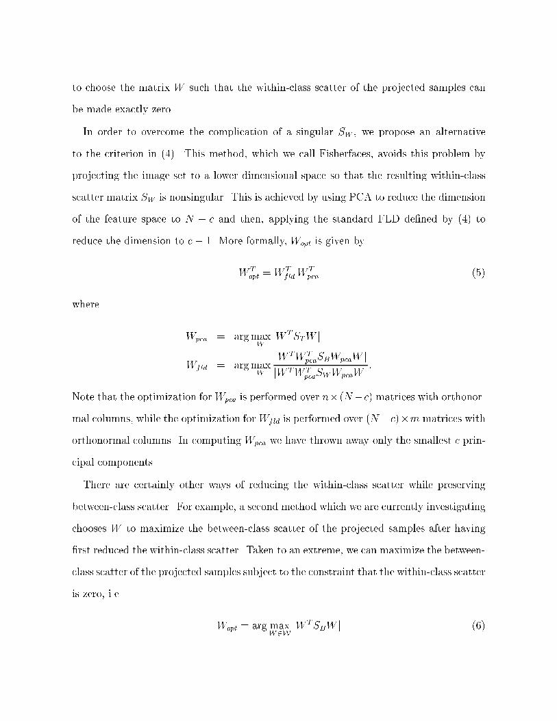
In order to overcome the complication of a singular SW , we propose an alternative
to the criterion in (4). This method, which we call Fisherfaces, avoids this problem by
projecting the image set to a lower dimensional space so that the resulting within-class
scatter matrix SW is nonsingular. This is achieved by using PCA to reduce the dimension
of the feature space to N � c and then, applying the standard FLD de�ned by (4) to
reduce the dimension to c� 1. More formally, Wopt is given by
W Topt =W T
fldWTpca (5)
where
Wpca = argmaxW
jW TSTW j
Wfld = argmaxW
jW TW TpcaSBWpcaW j
jW TW TpcaSWWpcaW j
:
Note that the optimization forWpca is performed over n�(N�c) matrices with orthonor-
mal columns, while the optimization forWfld is performed over (N�c)�m matrices with
orthonormal columns. In computing Wpca we have thrown away only the smallest c prin-
cipal components.
There are certainly other ways of reducing the within-class scatter while preserving
between-class scatter. For example, a second method which we are currently investigating
chooses W to maximize the between-class scatter of the projected samples after having
�rst reduced the within-class scatter. Taken to an extreme, we can maximize the between-
class scatter of the projected samples subject to the constraint that the within-class scatter
is zero, i.e.
Wopt = arg maxW2W
jW TSBW j (6)

where W is the set of n�m matrices with orthonormal columns contained in the kernel
of SW .
3 Experimental Results
In this section we present and discuss each of the aforementioned face recognition tech-
niques using two di�erent databases. Because of the speci�c hypotheses that we wanted
to test about the relative performance of the considered algorithms, many of the standard
databases were inappropriate. So we have used a database from the Harvard Robotics
Laboratory in which lighting has been systematically varied. Secondly, we have con-
structed a database at Yale that includes variation in both facial expression and lighting.1
3.1 Variation in Lighting
The �rst experiment was designed to test the hypothesis that under variable illumination,
face recognition algorithms will perform better if they exploit the fact that images of a
Lambertian surface lie in a linear subspace. More speci�cally, the recognition error rates
for all four algorithms described in Section 2 are compared using an image database
constructed by Hallinan at the Harvard Robotics Laboratory [14, 15]. In each image in
this database, a subject held his/her head steady while being illuminated by a dominant
light source. The space of light source directions, which can be parameterized by spherical
angles, was then sampled in 15� increments. See Figure 3. From this database, we used
330 images of �ve people (66 of each). We extracted �ve subsets to quantify the e�ects
of varying lighting. Sample images from each subset are shown in Fig. 4.
Subset 1 contains 30 images for which both of the longitudinal and latitudinal angles
of light source direction are within 15� of the camera axis, including the lighting
1The Yale database is available for download from http://cvc.yale.edu.

Subset 1 Subset 2 Subset 3 Subset 4 Subset 5
Figure 3. The highlighted lines of longitude and latitude indicate the light source directionsfor Subsets 1 through 5. Each intersection of a longitudinal and latitudinal line on the right sideof the illustration has a corresponding image in the database.
Subset 1 Subset 2 Subset 3 Subset 4 Subset 5
Figure 4. Example images from each subset of the Harvard Database used to test the fouralgorithms.
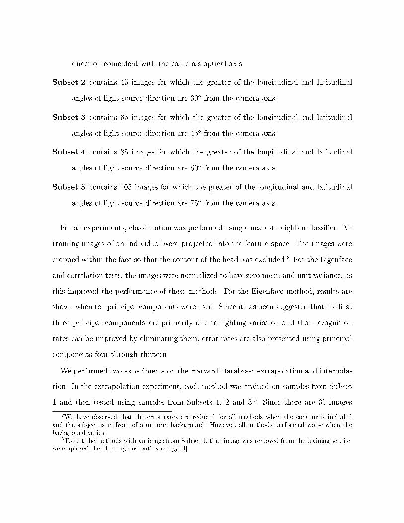
direction coincident with the camera's optical axis.
Subset 2 contains 45 images for which the greater of the longitudinal and latitudinal
angles of light source direction are 30� from the camera axis.
Subset 3 contains 65 images for which the greater of the longitudinal and latitudinal
angles of light source direction are 45� from the camera axis.
Subset 4 contains 85 images for which the greater of the longitudinal and latitudinal
angles of light source direction are 60� from the camera axis.
Subset 5 contains 105 images for which the greater of the longitudinal and latitudinal
angles of light source direction are 75� from the camera axis.
For all experiments, classi�cation was performed using a nearest neighbor classi�er. All
training images of an individual were projected into the feature space. The images were
cropped within the face so that the contour of the head was excluded.2 For the Eigenface
and correlation tests, the images were normalized to have zero mean and unit variance, as
this improved the performance of these methods. For the Eigenface method, results are
shown when ten principal components were used. Since it has been suggested that the �rst
three principal components are primarily due to lighting variation and that recognition
rates can be improved by eliminating them, error rates are also presented using principal
components four through thirteen.
We performed two experiments on the Harvard Database: extrapolation and interpola-
tion. In the extrapolation experiment, each method was trained on samples from Subset
1 and then tested using samples from Subsets 1, 2 and 3.3 Since there are 30 images
2We have observed that the error rates are reduced for all methods when the contour is included
and the subject is in front of a uniform background. However, all methods performed worse when the
background varies.3To test the methods with an image from Subset 1, that image was removed from the training set, i.e.
we employed the \leaving-one-out" strategy [4].

0
5
10
15
20
25
30
35
40
45
Subset 1 Subset 2 Subset 3
Lighting Direction Subset
Error
rate
Eigenface (10)
Eigenface (10) w/o first 3
Correlation
Linear Subspace
Fisherface
Eigenface (10)
Correlation
Eigenface (10)w/o first 3
LinearSubspace
Fisherface(%)
Extrapolating from Subset 1
Method Reduced Error Rate (%)
Space Subset 1 Subset 2 Subset 3
Eigenface4 0.0 31.1 47.7
10 0.0 4.4 41.5
Eigenface 4 0.0 13.3 41.5
w/o 1st 3 10 0.0 4.4 27.7
Correlation 29 0.0 0.0 33.9
Linear Subspace 15 0.0 4.4 9.2
Fisherface 4 0.0 0.0 4.6
Figure 5. Extrapolation: When each of the methods is trained on images with near frontalillumination (Subset 1), the graph and corresponding table show the relative performance underextreme light source conditions.
in the training set, correlation is equivalent to the Eigenface method using 29 principal
components. Figure 5 shows the result from this experiment.
In the interpolation experiment, each method was trained on Subsets 1 and 5 and then
tested the methods on Subsets 2, 3 and 4. Figure 6 shows the result from this experiment.
These two experiments reveal a number of interesting points:
1. All of the algorithms perform perfectly when lighting is nearly frontal. However as

0
5
10
15
20
25
30
35
Subset 2 Subset 3 Subset 4
Lighting Direction Subset
Error
rate
Eigenface (10)
Correlation
Eigenface (10)w/o first 3
LinearSubspace
Fisherface(%)
Interpolating between Subsets 1 and 5
Method Reduced Error Rate (%)
Space Subset 2 Subset 3 Subset 4
Eigenface4 53.3 75.4 52.9
10 11.11 33.9 20.0
Eigenface 4 31.11 60.0 29.4
w/o 1st 3 10 6.7 20.0 12.9
Correlation 129 0.0 21.54 7.1
Linear Subspace 15 0.0 1.5 0.0
Fisherface 4 0.0 0.0 1.2
Figure 6. Interpolation: When each of the methods is trained on images from both nearfrontal and extreme lighting (Subsets 1 and 5), the graph and corresponding table show therelative performance under intermediate lighting conditions.

lighting is moved o� axis, there is a signi�cant performance di�erence between the
two class-speci�c methods and the Eigenface method.
2. It has also been noted that the Eigenface method is equivalent to correlation when
the number of Eigenfaces equals the size of the training set [17], and since perfor-
mance increases with the dimension of the Eigenspace, the Eigenface method should
do no better than correlation [26]. This is empirically demonstrated as well.
3. In the Eigenface method, removing the �rst three principal components results in
better performance under variable lighting conditions.
4. While the Linear Subspace method has error rates that are competitive with the
Fisherface method, it requires storing more than three times as much information
and takes three times as long.
5. The Fisherface method had error rates lower than the Eigenface method and re-
quired less computation time.
3.2 Variation in Facial Expression, Eye Wear, and Lighting
Figure 7. The Yale database contains 160 frontal face images covering sixteen individualstaken under ten di�erent conditions: A normal image under ambient lighting, one with orwithout glasses, three images taken with di�erent point light sources, and �ve di�erent facialexpressions.
Using a second database constructed at the Yale Center for Computational Vision and
Control, we designed tests to determine how the methods compared under a di�erent range
of conditions. For sixteen subjects, ten images were acquired during one session in front
of a simple background. Subjects included females and males (some with facial hair), and
some wore glasses. Figure 7 shows ten images of one subject. The �rst image was taken

0
5
10
15
20
25
30
35
0 50 100 150
Number of Principal Components
Error
Rate
Eigenface
Eigenface w/o firstthree components
Fisherface (7.3%)
(%)
Figure 8. As demonstrated on the Yale Database, the variation in performance of the Eigenfacemethod depends on the number of principal components retained. Dropping the �rst threeappears to improve performance.
under ambient lighting in a neutral facial expression and the person wore glasses. In the
second image, the glasses were removed. If the person normally wore glasses, those were
used; if not, a random pair was borrowed. Images 3-5 were acquired by illuminating the
face in a neutral expression with a Luxolamp in three position. The last �ve images were
acquired under ambient lighting with di�erent expressions (happy, sad, winking, sleepy,
and surprised). For the Eigenface and correlation tests, the images were normalized to
have zero mean and unit variance, as this improved the performance of these methods.
The images were manually centered and cropped to two di�erent scales: The larger images
included the full face and part of the background while the closely cropped ones included
internal structures such as the brow, eyes, nose, mouth and chin but did not extend to
the occluding contour.
In this test, error rates were determined by the \leaving-one-out" strategy [4]: To
classify an image of a person, that image was removed from the data set and the dimen-
sionality reduction matrix W was computed. All images in the database, excluding the

test image, were then projected down into the reduced space to be used for classi�cation.
Recognition was performed using a nearest neighbor classi�er. Note that for this test,
each person in the learning set is represented by the projection of ten images, except for
the test person who is represented by only nine.
In general, the performance of the Eigenface method varies with the number of principal
components. Thus, before comparing the Linear Subspace and Fisherface methods with
the Eigenface method, we �rst performed an experiment to determine the number of
principal components yielding the lowest error rate. Figure 8 shows a plot of error rate
vs. the number of principal components, for the closely cropped set, when the initial three
principal components were retained and when they were dropped.
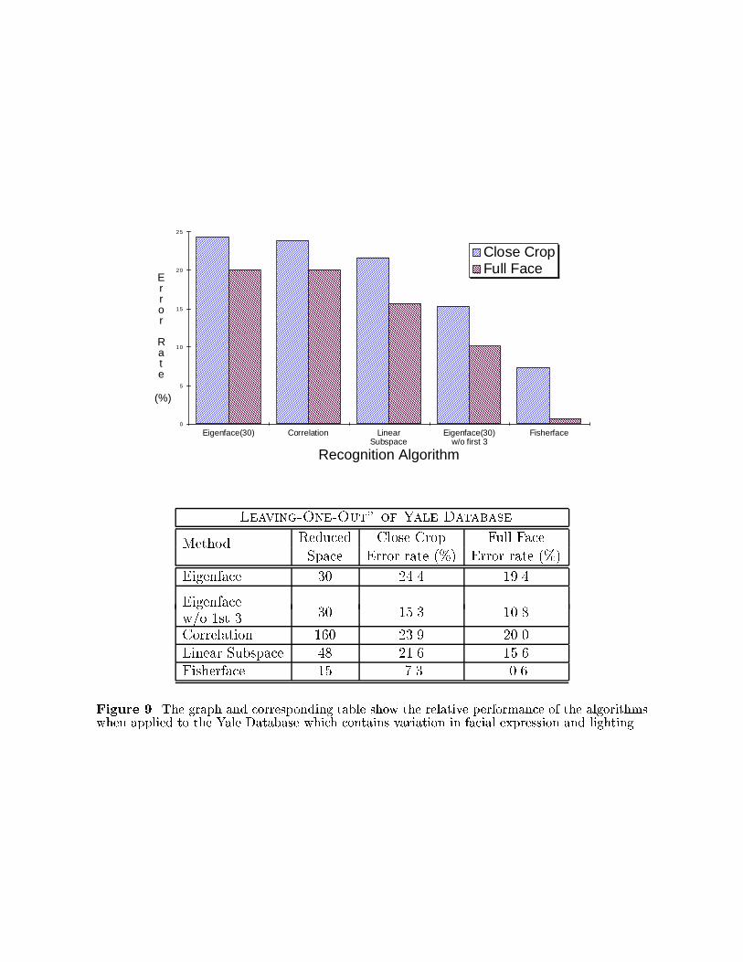
The relative performance of the algorithms is self evident in Fig. 9. The Fisherface
method had error rates that were better than half that of any other method. It seems
that the Fisherface method chooses the set of projections which performs well over a range
of lighting variation, facial expression variation, and presence of glasses.
Note that the Linear Subspace method faired comparatively worse in this experiment
than in the lighting experiments in the previous section. Because of variation in facial
expression, the images no longer lie in a linear subspace. Since the Fisherface method
tends to discount those portions of the image that are not signi�cant for recognizing an
individual, the resulting projections W tend to mask the regions of the face that are
highly variable. For example, the area around the mouth is discounted since it varies
quite a bit for di�erent facial expressions. On the other hand, the nose, cheeks and brow
are stable over the within-class variation and are more signi�cant for recognition. Thus,
we conjecture that Fisherface methods, which tend to reduce within-class scatter for all
classes, should produce projection directions that are also good for recognizing other faces
besides the training set.
0
5
10
15
20
25
Eigenface(30) Correlation LinearSubspace
Eigenface(30)w/o first 3
Fisherface
Recognition Algorithm
Error
Rate
Close CropFull Face
(%)
\Leaving-One-Out" of Yale Database
Method Reduced Close Crop Full Face
Space Error rate (%) Error rate (%)
Eigenface 30 24.4 19.4
Eigenfacew/o 1st 3 30 15.3 10.8
Correlation 160 23.9 20.0
Linear Subspace 48 21.6 15.6
Fisherface 15 7.3 0.6
Figure 9. The graph and corresponding table show the relative performance of the algorithmswhen applied to the Yale Database which contains variation in facial expression and lighting.
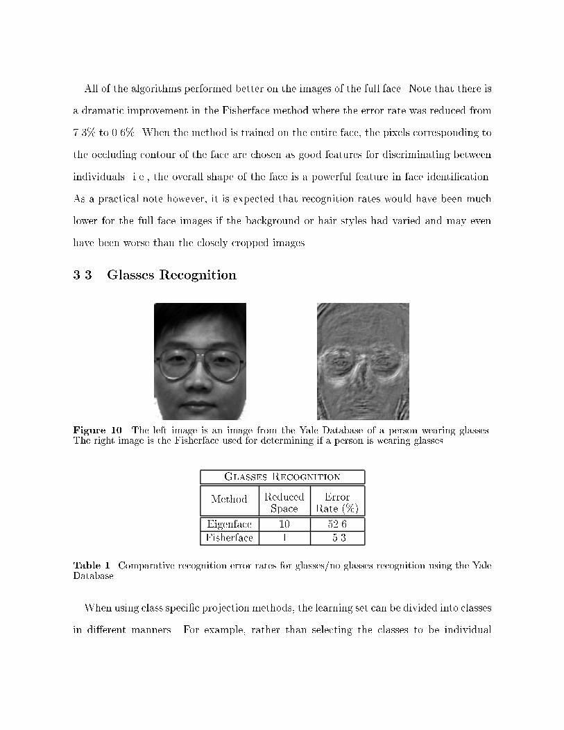
All of the algorithms performed better on the images of the full face. Note that there is
a dramatic improvement in the Fisherface method where the error rate was reduced from
7.3% to 0.6%. When the method is trained on the entire face, the pixels corresponding to
the occluding contour of the face are chosen as good features for discriminating between
individuals. i.e., the overall shape of the face is a powerful feature in face identi�cation.
As a practical note however, it is expected that recognition rates would have been much
lower for the full face images if the background or hair styles had varied and may even
have been worse than the closely cropped images.
3.3 Glasses Recognition
Figure 10. The left image is an image from the Yale Database of a person wearing glasses.The right image is the Fisherface used for determining if a person is wearing glasses.
Glasses Recognition
Method Reduced ErrorSpace Rate (%)
Eigenface 10 52.6
Fisherface 1 5.3
Table 1. Comparative recognition error rates for glasses/no glasses recognition using the YaleDatabase.
When using class speci�c projection methods, the learning set can be divided into classes
in di�erent manners. For example, rather than selecting the classes to be individual

people, the set of images can be divided into two classes: \wearing glasses" and \not
wearing glasses." With only two classes, the images can be projected to a line using the
Fisherface methods. Using PCA, the choice of the Eigenfaces is independent of the class
de�nition.
In this experiment, the data set contained 36 images from a superset of the Yale
Database, half with glasses. The recognition rates were obtained by cross validation,
i.e. to classify the images of each person, all images of that person were removed from
the database before the projection matrix W was computed. Table 1 presents the error
rates for three di�erent methods.
PCA had recognition rates near chance since in most cases it classi�ed both images
with and without glasses to the same class. On the other hand, the Fisherface methods
can be viewed as deriving a template which is suited for �nding glasses and ignoring other
characteristics of the face. This conjecture is supported by observing the Fisherface in
Fig. 10 corresponding to the projection matrixW . Naturally, it is expected that the same
techniques could be applied to identifying facial expressions where the set of training
images is divided into classes based on the facial expression.
4 Conclusion
The experiments suggest a number of conclusions:
1. All methods perform well if presented with an image in the test set which is similar
to an image in the training set.
2. The Fisherface method appears to be the best at extrapolating and interpolating
over variation in lighting, although the Linear Subspace method is a close second.
3. Removing the largest three principal components does improve the performance of

the Eigenface method in the presence of lighting variation, but does not achieve
error rates as low as some of the other methods described here.
4. In the limit as more principal components are used in the Eigenface method, per-
formance approaches that of correlation. Similarly, when the �rst three principal
components have been removed, performance improves as the dimensionality of the
feature space is increased. Note however, that performance seems to level o� at
about 45 principal components. Sirovitch and Kirby found a similar point of dimin-
ishing returns when using Eigenfaces to represent face images [6].
5. The Fisherface method appears to be the best at simultaneously handling variation
in lighting and expression. As expected, the Linear Subspace method su�ers when
confronted with variation in facial expression.
Even with this extensive experimentation, interesting questions remain: How well does
the Fisherface method extend to large databases. Can variation in lighting conditions be
accommodated if some of the individuals are only observed under one lighting condition?
Additionally, current face detection methods are likely to break down under extreme
lighting conditions such as Subsets 4 and 5 in Fig. 4, and so new detection methods are
needed to support the algorithms presented in this paper. Finally, when shadowing domi-
nates, performance degrades for all of the presented recognition methods, and techniques
that either model or mask the shadowed regions may be needed. We are currently investi-
gating models for representing the set of images of an object under all possible illumination
conditions, and have shown that the set of n-pixel images of an object of any shape and
with an arbitrary re ectance function, seen under all possible illumination conditions,
forms a convex cone in IRn [32]. Furthermore, and most relevant to this paper, it appears
that this convex illumination cone lies close to a low-dimensional linear subspace [14].

Acknowledgments
P.N. Belhumeur was supported by ARO grant DAAH04-95-1-0494. J.P. Hespanha was
supported by NSF Grant ECS-9206021, AFOSR Grant F49620-94-1-0181, and AROGrant
DAAH04-95-1-0114. D.J. Kriegman was supported by NSF under an NYI, IRI-9257990
and by ONR N00014-93-1-0305. The authors would like to thank Peter Hallinan for
providing the Harvard Database, and Alan Yuille and David Mumford for many useful
discussions.

List of Figures
1 The same person seen under di�erent lighting conditions can appear dra-
matically di�erent: In the left image, the dominant light source is nearly
head-on; in the right image, the dominant light source is from above and
to the right. . . . . . . . . . . . . . . . . . . . . . . . . . . . . . . . . . . . 3
2 A comparison of principal component analysis (PCA) and Fisher's linear
discriminant (FLD) for a two class problem where data for each class lies
near a linear subspace. . . . . . . . . . . . . . . . . . . . . . . . . . . . . 11
3 The highlighted lines of longitude and latitude indicate the light source
directions for Subsets 1 through 5. Each intersection of a longitudinal and
latitudinal line on the right side of the illustration has a corresponding
image in the database. . . . . . . . . . . . . . . . . . . . . . . . . . . . . . 15
4 Example images from each subset of the Harvard Database used to test the
four algorithms. . . . . . . . . . . . . . . . . . . . . . . . . . . . . . . . . . 15
5 Extrapolation: When each of the methods is trained on images with near
frontal illumination (Subset 1), the graph and corresponding table show the
relative performance under extreme light source conditions. . . . . . . . . . 17
6 Interpolation: When each of the methods is trained on images from both
near frontal and extreme lighting (Subsets 1 and 5), the graph and corre-
sponding table show the relative performance under intermediate lighting
conditions. . . . . . . . . . . . . . . . . . . . . . . . . . . . . . . . . . . . . 18
7 The Yale database contains 160 frontal face images covering sixteen individ-
uals taken under ten di�erent conditions: A normal image under ambient
lighting, one with or without glasses, three images taken with di�erent
point light sources, and �ve di�erent facial expressions. . . . . . . . . . . 19

8 As demonstrated on the Yale Database, the variation in performance of
the Eigenface method depends on the number of principal components
retained. Dropping the �rst three appears to improve performance. . . . . 20
9 The graph and corresponding table show the relative performance of the
algorithms when applied to the Yale Database which contains variation in
facial expression and lighting. . . . . . . . . . . . . . . . . . . . . . . . . . 22
10 The left image is an image from the Yale Database of a person wearing
glasses. The right image is the Fisherface used for determining if a person
is wearing glasses. . . . . . . . . . . . . . . . . . . . . . . . . . . . . . . . . 23
List of Tables
1 Comparative recognition error rates for glasses/no glasses recognition using
the Yale Database. . . . . . . . . . . . . . . . . . . . . . . . . . . . . . . . 23

Footnotes
1. The Yale database is available for download from http://cvc.yale.edu.
2. We have observed that the error rates are reduced for all methods when the contour
is included and the subject is in front of a uniform background. However, all methods
performed worse when the background varies.
3. To test the methods with an image from Subset 1, that image was removed from
the training set, i.e. we employed the \leaving-one-out" strategy [4].

Contact Information
� Peter N. Belhumeur, Center for Computational Vision and Control, Dept. of Electri-
cal Engineering, Yale University, New Haven, CT 06520-8267, Phone: 203-432-4249,
Fax: 203-432-7481, [email protected].
� Jo~ao P. Hespanha, Center for Computational Vision and Control, Dept. of Electrical
Engineering, Yale University, New Haven, CT 06520-8267, Phone: 203-432-7061,
Fax: 203-432-7481, [email protected].
� David J. Kriegman, Center for Computational Vision and Control, Dept. of Electri-
cal Engineering, Yale University, New Haven, CT 06520-8267, Phone: 203-432-4091,
Fax: 203-432-7481, [email protected].

References
[1] R. Chellappa, C. Wilson, and S. Sirohey, \Human and machine recognition of faces:
A survey", Proceedings of the IEEE, vol. 83, no. 5, pp. 705{740, 1995.
[2] A. Samal and P. Iyengar, \Automatic recognition and analysis of human faces and
facial expressions: A survey", Pattern Recognition, vol. 25, pp. 65{77, 1992.
[3] Amnon Shashua, Geometry and Photometry in 3D Visual Recognition, PhD thesis,
MIT, 1992.
[4] R. Duda and P. Hart, Pattern Classi�cation and Scene Analysis, Wiley, New York,
1973.
[5] R.A. Fisher, \The use of multiple measures in taxonomic problems", Ann. Eugenics,
vol. 7, pp. 179{188, 1936.
[6] L. Sirovitch and M. Kirby, \Low-dimensional procedure for the characterization of
human faces", J. Optical Soc. of America A, vol. 2, pp. 519{524, 1987.
[7] M. Turk and A. Pentland, \Eigenfaces for recognition", J. of Cognitive Neuroscience,
vol. 3, no. 1, 1991.
[8] M. Turk and A. Pentland, \Face recognition using eigenfaces", in Proc. IEEE Conf.
on Comp. Vision and Patt. Recog., 1991, pp. 586{591.
[9] Y. Moses, Y. Adini, and S. Ullman, \Face recognition: The problem of compensating
for changes in illumination direction", in European Conf. on Computer Vision, 1994,
pp. 286{296.

[10] Y. Cheng, K. Liu, J. Yang, Y. Zhuang, and N. Gu, \Human face recognition method
based on the statistical model of small sample size", in SPIE Proc.: Intelligent Robots
and Computer Vision X: Algorithms and Techn., 1991, pp. 85{95.
[11] S. Baker and S.K. Nayar, \Pattern rejection", in Proc. IEEE Conf. on Comp. Vision
and Patt. Recog., 1996, pp. 544{549.
[12] P. N. Belhumeur, J. P. Hespanha, and D. J. Kriegman, \Eigenfaces vs. Fisherfaces:
Recognition using class speci�c linear projection", in European Conf. on Computer
Vision, 1996, pp. 45{58.
[13] Y. Cui, D. Swets, and J. Weng, \Learning-based hand sign recognition using
SHOSLIF-M", in Int. Conf. on Computer Vision, 1995, pp. 631{636.
[14] Peter Hallinan, \A low-dimensional representation of human faces for arbitrary light-
ing conditions", in Proc. IEEE Conf. on Comp. Vision and Patt. Recog., 1994, pp.
995{999.
[15] Peter Hallinan, A Deformable Model for Face Recognition Under Arbitrary Lighting
Conditions, PhD thesis, Harvard University, 1995.
[16] A. Pentland, B. Moghaddam, and Starner, \View-based and modular eigenspaces for
face recognition", in Proc. IEEE Conf. Computer Vision and Pattern Recognition,
1994, pp. 84{91.
[17] H. Murase and S. Nayar, \Visual learning and recognition of 3-D objects from
appearence", Int. J. Computer Vision, vol. 14, no. 5{24, 1995.
[18] D. Beymer, \Face recognition under varying pose", in Proc. IEEE Conf. Computer
Vision and Pattern Recognition, 1994, pp. 756{761.

[19] A. Gee and R. Cipolla, \Determining the gaze of faces in images", Image and Vision
Computing, vol. 12, pp. 639{648, 1994.
[20] A. Lanitis, C.J. Taylor, and T.F. Cootes, \A uni�ed approach to coding and inter-
preting face images", in Int. Conf. on Computer Vision, 1995, pp. 368{373.
[21] Q. Chen, H. Wu, and M. Yachida, \Face detection by fuzzy pattern matching", in
Int. Conf. on Computer Vision, 1995, pp. 591{596.
[22] I. Craw, D. Tock, and A. Bennet, \Finding face features", in Proc. European Conf.
on Computer Vision, 1992, pp. 92{96.
[23] T. Leung, M. Burl, and P. Perona, \Finding faces in cluttered scenes using labeled
random graph matching", in Int. Conf. on Computer Vision, 1995, pp. 637{644.
[24] K. Matsuno, C.W. Lee, S. Kimura, and S. Tsuji, \Automatic recognition of human
facial expressions", in Int. Conf. on Computer Vision, 1995, pp. 352{359.
[25] Moghaddam and Pentland, \Probabilistic visual learning for object detection", in
Int. Conf. on Computer Vision, 1995, pp. 786{793.
[26] R. Brunelli and T. Poggio, \Face recognition: Features vs templates", IEEE Trans.
Pattern Anal. Mach. Intelligence, vol. 15, no. 10, pp. 1042{1053, 1993.
[27] J.M. Gilbert and W. Yang, \A Real{Time Face Recognition System Using Custom
VLSI Hardware", in Proceedings of IEEE Workshop on Computer Architectures for
Machine Perception, 1993, pp. 58{66.
[28] B.K.P. Horn, Computer Vision, MIT Press, Cambridge, Mass., 1986.
[29] W.M. Silver, Determining Shape and Re ectance Using Multiple Images, PhD thesis,
MIT, Cambridge, MA, 1980.

[30] R.J. Woodham, \Analysing images of curved surfaces", Arti�cial Intelligence, vol.
17, pp. 117{140, 1981.
[31] S. Nayar and H. Murase, \Dimensionality of illumination in appearance matching",
IEEE Conf. on Robotics and Automation, 1996.
[32] P.N. Belhumeur and D.J. Kriegman, \What is the set of images of an object under
all possible lighting conditions?", in IEEE Proc. Conf. Computer Vision and Pattern
Recognition, 1996.
Top Related