IBM SPSS Conjoint 19IBM SPSS Conjoint 19
Note: Before using this information and the product it supports, read the general information under Notices on p. 39. This document contains proprietary information of SPSS Inc, an IBM Company. It is provided under a license agreement and is protected by copyright law. The information contained in this publication does not include any product warranties, and any statements provided in this manual should not be interpreted as such. When you send information to IBM or SPSS, you grant IBM and SPSS a nonexclusive right to use or distribute the information in any way it believes appropriate without incurring any obligation to you.
© Copyright SPSS Inc. 1989, 2010.
Preface
IBM® SPSS® Statistics is a comprehensive system for analyzing data. The Conjoint optional add-on module provides the additional analytic techniques described in this manual. The Conjoint add-on module must be used with the SPSS Statistics Core system and is completely integrated into that system.
About SPSS Inc., an IBM Company
SPSS Inc., an IBM Company, is a leading global provider of predictive analytic software and solutions. The company’s complete portfolio of products — data collection, statistics, modeling and deployment — captures people’s attitudes and opinions, predicts outcomes of future customer interactions, and then acts on these insights by embedding analytics into business processes. SPSS Inc. solutions address interconnected business objectives across an entire organization by focusing on the convergence of analytics, IT architecture, and business processes. Commercial, government, and academic customers worldwide rely on SPSS Inc. technology as a competitive advantage in attracting, retaining, and growing customers, while reducing fraud and mitigating risk. SPSS Inc. was acquired by IBM in October 2009. For more information, visit http://www.spss.com.
Technical support
Technical support is available to maintenance customers. Customers may contact Technical Support for assistance in using SPSS Inc. products or for installation help for one of the supported hardware environments. To reach Technical Support, see the SPSS Inc. web site at http://support.spss.com or find your local office via the web site at http://support.spss.com/default.asp?refpage=contactus.asp. Be prepared to identify yourself, your organization, and your support agreement when requesting assistance.
Customer Service
If you have any questions concerning your shipment or account, contact your local office, listed on the Web site at http://www.spss.com/worldwide. Please have your serial number ready for identification.
Training Seminars
SPSS Inc. provides both public and onsite training seminars. All seminars feature hands-on workshops. Seminars will be offered in major cities on a regular basis. For more information on these seminars, contact your local office, listed on the Web site at http://www.spss.com/worldwide.
© Copyright SPSS Inc. 1989, 2010 iii
The SPSS Statistics: Guide to Data Analysis, SPSS Statistics: Statistical Procedures Companion, and SPSS Statistics: Advanced Statistical Procedures Companion, written by Marija Norušis and published by Prentice Hall, are available as suggested supplemental material. These publications cover statistical procedures in the SPSS Statistics Base module, Advanced Statistics module and Regression module. Whether you are just getting starting in data analysis or are ready for advanced applications, these books will help you make best use of the capabilities found within the IBM® SPSS® Statistics offering. For additional information including publication contents and sample chapters, please see the author’s website: http://www.norusis.com
1 Introduction to Conjoint Analysis 1
The Full-Profile Approach . . . . . . . . . . . . . . . . . . . . . . . . . . . . . . . . . . . . . . . . . . . . . . . . . . . . . . . 2 An Orthogonal Array . . . . . . . . . . . . . . . . . . . . . . . . . . . . . . . . . . . . . . . . . . . . . . . . . . . . . . . 2 The Experimental Stimuli . . . . . . . . . . . . . . . . . . . . . . . . . . . . . . . . . . . . . . . . . . . . . . . . . . . . 2 Collecting and Analyzing the Data . . . . . . . . . . . . . . . . . . . . . . . . . . . . . . . . . . . . . . . . . . . . . 2
Part I: User’s Guide
2 Generating an Orthogonal Design 5
Defining Values for an Orthogonal Design . . . . . . . . . . . . . . . . . . . . . . . . . . . . . . . . . . . . . . . . . . . 6 Orthogonal Design Options . . . . . . . . . . . . . . . . . . . . . . . . . . . . . . . . . . . . . . . . . . . . . . . . . . . . . . 7 ORTHOPLAN Command Additional Features . . . . . . . . . . . . . . . . . . . . . . . . . . . . . . . . . . . . . . . . . 8
3 Displaying a Design 9
Display Design Titles. . . . . . . . . . . . . . . . . . . . . . . . . . . . . . . . . . . . . . . . . . . . . . . . . . . . . . . . . . . 10 PLANCARDS Command Additional Features . . . . . . . . . . . . . . . . . . . . . . . . . . . . . . . . . . . . . . . . . 10
4 Running a Conjoint Analysis 11
Requirements . . . . . . . . . . . . . . . . . . . . . . . . . . . . . . . . . . . . . . . . . . . . . . . . . . . . . . . . . . . . . . . 11 Specifying the Plan File and the Data File. . . . . . . . . . . . . . . . . . . . . . . . . . . . . . . . . . . . . . . . 12 Specifying How Data Were Recorded . . . . . . . . . . . . . . . . . . . . . . . . . . . . . . . . . . . . . . . . . . 12
Optional Subcommands . . . . . . . . . . . . . . . . . . . . . . . . . . . . . . . . . . . . . . . . . . . . . . . . . . . . . . . . 13
5 Using Conjoint Analysis to Model Carpet-Cleaner Preference17
Generating an Orthogonal Design . . . . . . . . . . . . . . . . . . . . . . . . . . . . . . . . . . . . . . . . . . . . . . . . . 17 Creating the Experimental Stimuli: Displaying the Design . . . . . . . . . . . . . . . . . . . . . . . . . . . . . . . 21 Running the Analysis . . . . . . . . . . . . . . . . . . . . . . . . . . . . . . . . . . . . . . . . . . . . . . . . . . . . . . . . . . 23 Utility Scores . . . . . . . . . . . . . . . . . . . . . . . . . . . . . . . . . . . . . . . . . . . . . . . . . . . . . . . . . . . . . . . . 25 Coefficients . . . . . . . . . . . . . . . . . . . . . . . . . . . . . . . . . . . . . . . . . . . . . . . . . . . . . . . . . . . . . . . . . 25 Relative Importance . . . . . . . . . . . . . . . . . . . . . . . . . . . . . . . . . . . . . . . . . . . . . . . . . . . . . . . . . . . 26 Correlations . . . . . . . . . . . . . . . . . . . . . . . . . . . . . . . . . . . . . . . . . . . . . . . . . . . . . . . . . . . . . . . . . 27 Reversals . . . . . . . . . . . . . . . . . . . . . . . . . . . . . . . . . . . . . . . . . . . . . . . . . . . . . . . . . . . . . . . . . . . 27 Running Simulations . . . . . . . . . . . . . . . . . . . . . . . . . . . . . . . . . . . . . . . . . . . . . . . . . . . . . . . . . . . 28 Preference Probabilities of Simulations . . . . . . . . . . . . . . . . . . . . . . . . . . . . . . . . . . . . . . . . . . . . 28
Appendices
1 Introduction to Conjoint Analysis
Conjoint analysis is a market research tool for developing effective product design. Using conjoint analysis, the researcher can answer questions such as: What product attributes are important or unimportant to the consumer? What levels of product attributes are the most or least desirable in the consumer’s mind? What is the market share of preference for leading competitors’ products versus our existing or proposed product? The virtue of conjoint analysis is that it asks the respondent to make choices in the same fashion
as the consumer presumably does—by trading off features, one against another. For example, suppose that you want to book an airline flight. You have the choice of sitting in a
cramped seat or a spacious seat. If this were the only consideration, your choice would be clear. You would probably prefer a spacious seat. Or suppose you have a choice of ticket prices: $225 or $800. On price alone, taking nothing else into consideration, the lower price would be preferable. Finally, suppose you can take either a direct flight, which takes two hours, or a flight with one layover, which takes five hours. Most people would choose the direct flight. The drawback to the above approach is that choice alternatives are presented on single attributes
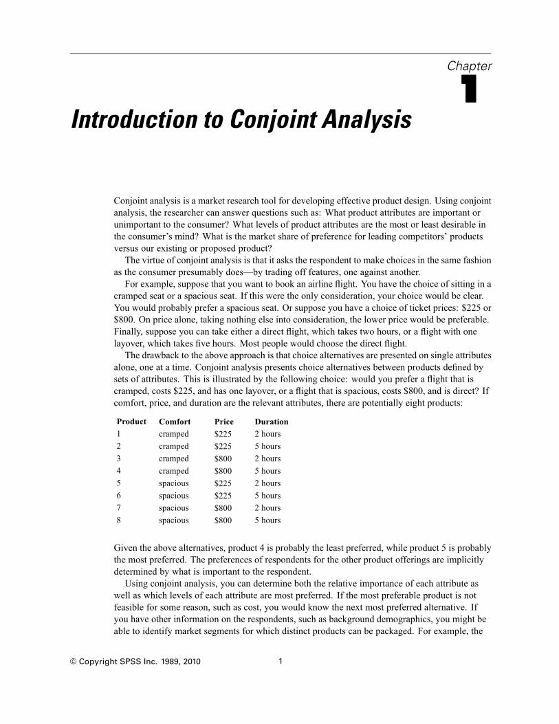
alone, one at a time. Conjoint analysis presents choice alternatives between products defined by sets of attributes. This is illustrated by the following choice: would you prefer a flight that is cramped, costs $225, and has one layover, or a flight that is spacious, costs $800, and is direct? If comfort, price, and duration are the relevant attributes, there are potentially eight products:
Product Comfort Price Duration 1 cramped $225 2 hours 2 cramped $225 5 hours 3 cramped $800 2 hours 4 cramped $800 5 hours 5 spacious $225 2 hours 6 spacious $225 5 hours 7 spacious $800 2 hours 8 spacious $800 5 hours
Given the above alternatives, product 4 is probably the least preferred, while product 5 is probably the most preferred. The preferences of respondents for the other product offerings are implicitly determined by what is important to the respondent. Using conjoint analysis, you can determine both the relative importance of each attribute as
well as which levels of each attribute are most preferred. If the most preferable product is not feasible for some reason, such as cost, you would know the next most preferred alternative. If you have other information on the respondents, such as background demographics, you might be able to identify market segments for which distinct products can be packaged. For example, the
© Copyright SPSS Inc. 1989, 2010 1
2
Chapter 1
business traveler and the student traveler might have different preferences that could be met by distinct product offerings.
The Full-Profile Approach
Conjoint uses the full-profile (also known as full-concept) approach, where respondents rank, order, or score a set of profiles, or cards, according to preference. Each profile describes a complete product or service and consists of a different combination of factor levels for all factors (attributes) of interest.
An Orthogonal Array
A potential problem with the full-profile approach soon becomes obvious if more than a few factors are involved and each factor has more than a couple of levels. The total number of profiles resulting from all possible combinations of the levels becomes too great for respondents to rank or score in a meaningful way. To solve this problem, the full-profile approach uses what is termed a fractional factorial design, which presents a suitable fraction of all possible combinations of the factor levels. The resulting set, called an orthogonal array, is designed to capture the main effects for each factor level. Interactions between levels of one factor with levels of another factor are assumed to be negligible. The Generate Orthogonal Design procedure is used to generate an orthogonal array and is
typically the starting point of a conjoint analysis. It also allows you to generate factor-level combinations, known as holdout cases, which are rated by the subjects but are not used to build the preference model. Instead, they are used as a check on the validity of the model.
The Experimental Stimuli
Each set of factor levels in an orthogonal design represents a different version of the product under study and should be presented to the subjects in the form of an individual product profile. This helps the respondent to focus on only the one product currently under evaluation. The stimuli should be standardized by making sure that the profiles are all similar in physical appearance except for the different combinations of features. Creation of the product profiles is facilitated with the Display Design procedure. It takes a
design generated by the Generate Orthogonal Design procedure, or entered by the user, and produces a set of product profiles in a ready-to-use format.
Collecting and Analyzing the Data
Since there is typically a great deal of between-subject variation in preferences, much of conjoint analysis focuses on the single subject. To generalize the results, a random sample of subjects from the target population is selected so that group results can be examined. The size of the sample in conjoint studies varies greatly. In one report (Cattin and Wittink,
1982), the authors state that the sample size in commercial conjoint studies usually ranges from 100 to 1,000, with 300 to 550 the most typical range. In another study (Akaah and Korgaonkar,
3
Introduction to Conjoint Analysis
1988), it is found that smaller sample sizes (less than 100) are typical. As always, the sample size should be large enough to ensure reliability. Once the sample is chosen, the researcher administers the set of profiles, or cards, to each
respondent. The Conjoint procedure allows for three methods of data recording. In the first method, subjects are asked to assign a preference score to each profile. This type of method is typical when a Likert scale is used or when the subjects are asked to assign a number from 1 to 100 to indicate preference. In the second method, subjects are asked to assign a rank to each profile ranging from 1 to the total number of profiles. In the third method, subjects are asked to sort the profiles in terms of preference. With this last method, the researcher records the profile numbers in the order given by each subject. Analysis of the data is done with the Conjoint procedure (available only through command
syntax) and results in a utility score, called a part-worth, for each factor level. These utility scores, analogous to regression coefficients, provide a quantitative measure of the preference for each factor level, with larger values corresponding to greater preference. Part-worths are expressed in a common unit, allowing them to be added together to give the total utility, or overall preference, for any combination of factor levels. The part-worths then constitute a model for predicting the preference of any product profile, including profiles, referred to as simulation cases, that were not actually presented in the experiment. The information obtained from a conjoint analysis can be applied to a wide variety of market
research questions. It can be used to investigate areas such as product design, market share, strategic advertising, cost-benefit analysis, and market segmentation. Although the focus of this manual is on market research applications, conjoint analysis can
be useful in almost any scientific or business field in which measuring people’s perceptions or judgments is important.
Part I: User’s Guide
Chapter
2 Generating an Orthogonal Design
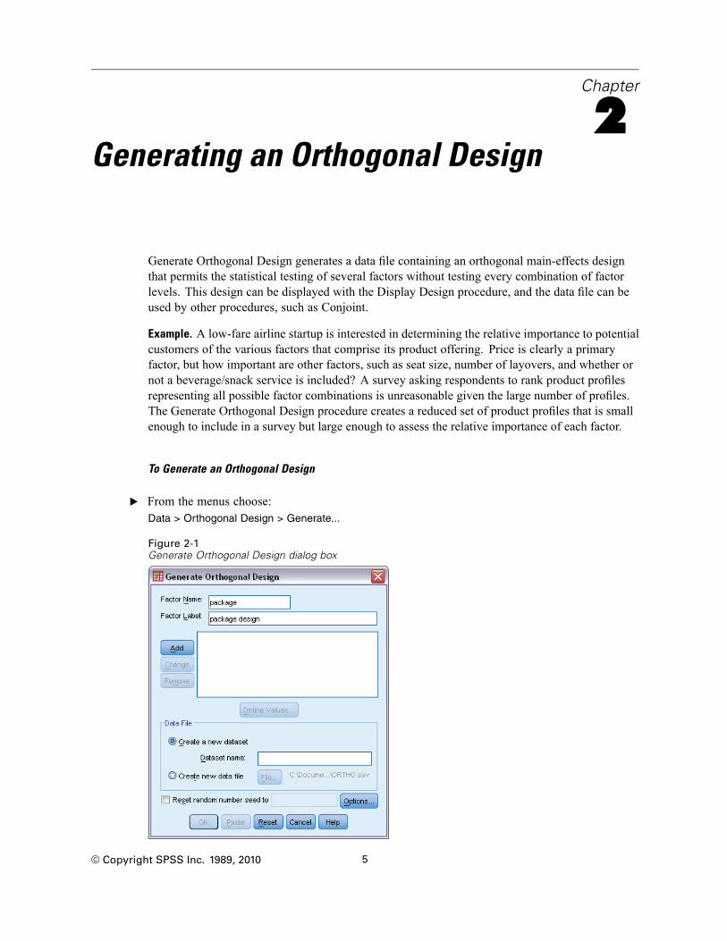
Generate Orthogonal Design generates a data file containing an orthogonal main-effects design that permits the statistical testing of several factors without testing every combination of factor levels. This design can be displayed with the Display Design procedure, and the data file can be used by other procedures, such as Conjoint.
Example. A low-fare airline startup is interested in determining the relative importance to potential customers of the various factors that comprise its product offering. Price is clearly a primary factor, but how important are other factors, such as seat size, number of layovers, and whether or not a beverage/snack service is included? A survey asking respondents to rank product profiles representing all possible factor combinations is unreasonable given the large number of profiles. The Generate Orthogonal Design procedure creates a reduced set of product profiles that is small enough to include in a survey but large enough to assess the relative importance of each factor.
To Generate an Orthogonal Design
E From the menus choose: Data > Orthogonal Design > Generate...
Figure 2-1 Generate Orthogonal Design dialog box
© Copyright SPSS Inc. 1989, 2010 5
6
Chapter 2
E Define at least one factor. Enter a name in the Factor Name text box. Factor names can be any valid variable name, except status_ or card_. You can also assign an optional factor label.
E Click Add to add the factor name and an optional label. To delete a factor, select it in the list and click Remove. To modify a factor name or label, select it in the list, modify the name or label, and click Change.
E Define values for each factor by selecting the factor and clicking Define Values.
Data File. Allows you to control the destination of the orthogonal design. You can save the design to a new dataset in the current session or to an external data file.
Create a new dataset. Creates a new dataset in the current session containing the factors and cases generated by the plan. Create new data file. Creates an external data file containing the factors and cases generated by the plan. By default, this data file is named ortho.sav, and it is saved to the current directory. Click File to specify a different name and destination for the file.
Reset random number seed to. Resets the random number seed to the specified value. The seed can be any integer value from 0 through 2,000,000,000. Within a session, a different seed is used each time you generate a set of random numbers, producing different results. If you want to duplicate the same random numbers, you should set the seed value before you generate your first design and reset the seed to the same value each subsequent time you generate the design.
Optionally, you can: Click Options to specify the minimum number of cases in the orthogonal design and to select holdout cases.
Defining Values for an Orthogonal Design Figure 2-2 Generate Design Define Values dialog box
7
Generating an Orthogonal Design
You must assign values to each level of the selected factor or factors. The factor name will be displayed after Values and Labels for. Enter each value of the factor. You can elect to give the values descriptive labels. If you do not
assign labels to the values, labels that correspond to the values are automatically assigned (that is, a value of 1 is assigned a label of 1, a value of 3 is assigned a label of 3, and so on).
Auto-Fill. Allows you to automatically fill the Value boxes with consecutive values beginning with 1. Enter the maximum value and click Fill to fill in the values.
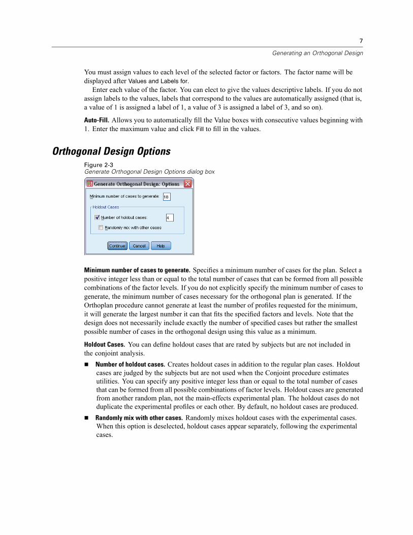
Orthogonal Design Options Figure 2-3 Generate Orthogonal Design Options dialog box
Minimum number of cases to generate. Specifies a minimum number of cases for the plan. Select a positive integer less than or equal to the total number of cases that can be formed from all possible combinations of the factor levels. If you do not explicitly specify the minimum number of cases to generate, the minimum number of cases necessary for the orthogonal plan is generated. If the Orthoplan procedure cannot generate at least the number of profiles requested for the minimum, it will generate the largest number it can that fits the specified factors and levels. Note that the design does not necessarily include exactly the number of specified cases but rather the smallest possible number of cases in the orthogonal design using this value as a minimum.
Holdout Cases. You can define holdout cases that are rated by subjects but are not included in the conjoint analysis.
Number of holdout cases. Creates holdout cases in addition to the regular plan cases. Holdout cases are judged by the subjects but are not used when the Conjoint procedure estimates utilities. You can specify any positive integer less than or equal to the total number of cases that can be formed from all possible combinations of factor levels. Holdout cases are generated from another random plan, not the main-effects experimental plan. The holdout cases do not duplicate the experimental profiles or each other. By default, no holdout cases are produced. Randomly mix with other cases. Randomly mixes holdout cases with the experimental cases. When this option is deselected, holdout cases appear separately, following the experimental cases.
8
ORTHOPLAN Command Additional Features
The command syntax language also allows you to: Append the orthogonal design to the active dataset rather than creating a new one. Specify simulation cases before generating the orthogonal design rather than after the design has been created.
See the Command Syntax Reference for complete syntax information.
Chapter
3 Displaying a Design
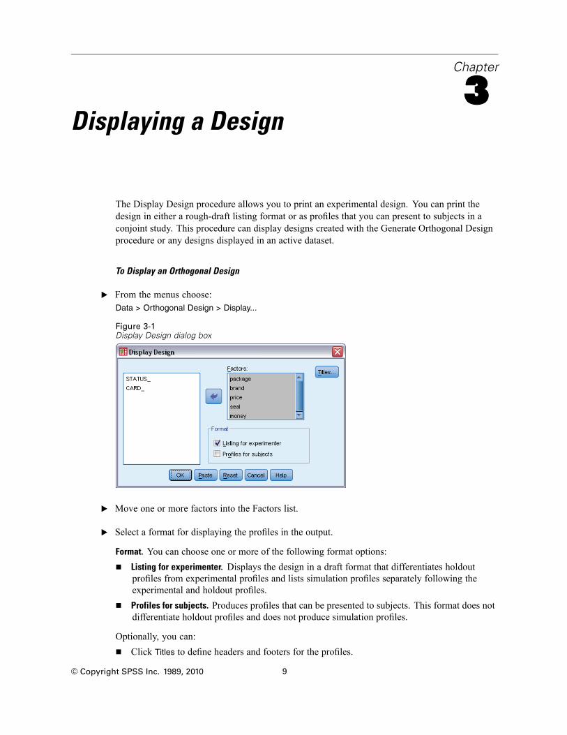
The Display Design procedure allows you to print an experimental design. You can print the design in either a rough-draft listing format or as profiles that you can present to subjects in a conjoint study. This procedure can display designs created with the Generate Orthogonal Design procedure or any designs displayed in an active dataset.
To Display an Orthogonal Design
E From the menus choose: Data > Orthogonal Design > Display...
Figure 3-1 Display Design dialog box
E Move one or more factors into the Factors list.
E Select a format for displaying the profiles in the output.
Format. You can choose one or more of the following format options: Listing for experimenter. Displays the design in a draft format that differentiates holdout profiles from experimental profiles and lists simulation profiles separately following the experimental and holdout profiles. Profiles for subjects. Produces profiles that can be presented to subjects. This format does not differentiate holdout profiles and does not produce simulation profiles.
Optionally, you can: Click Titles to define headers and footers for the profiles.
© Copyright SPSS Inc. 1989, 2010 9
10
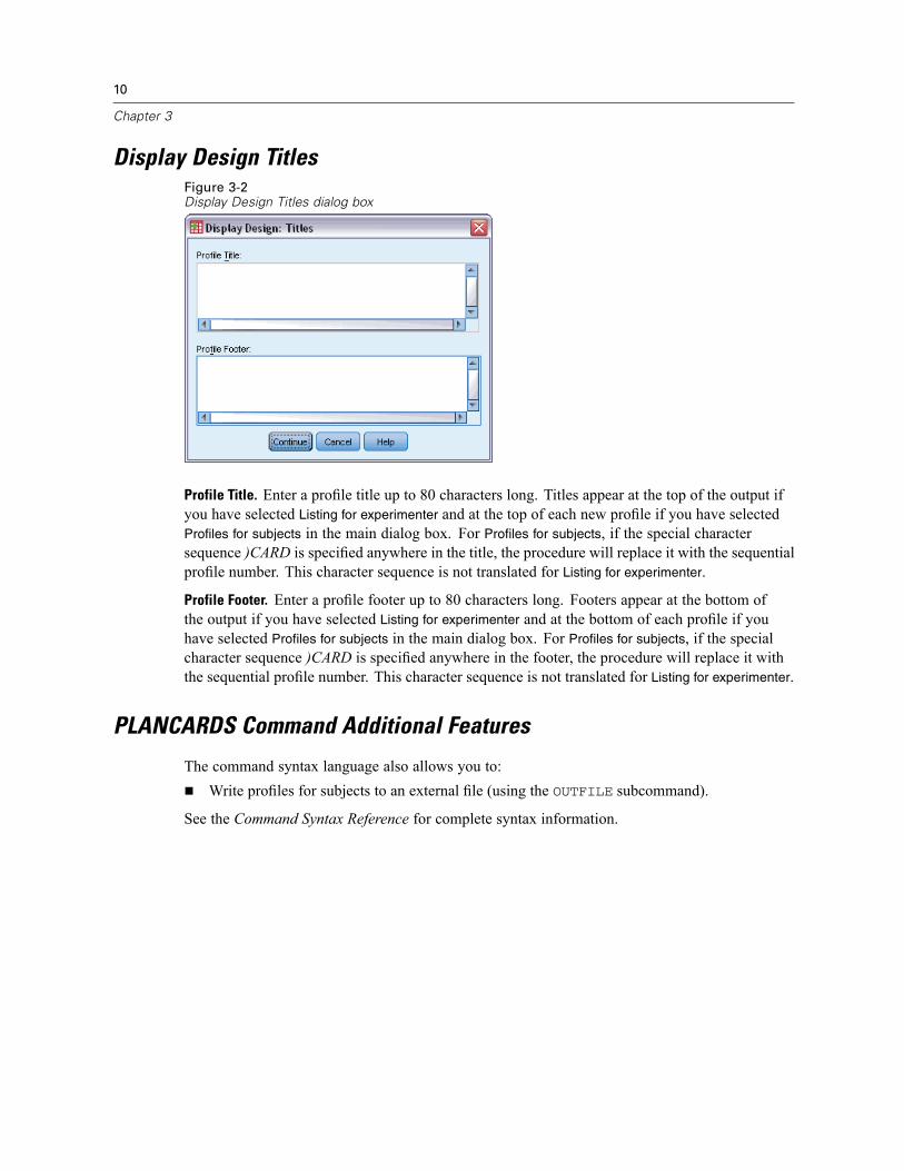
Display Design Titles Figure 3-2 Display Design Titles dialog box
Profile Title. Enter a profile title up to 80 characters long. Titles appear at the top of the output if you have selected Listing for experimenter and at the top of each new profile if you have selected Profiles for subjects in the main dialog box. For Profiles for subjects, if the special character sequence )CARD is specified anywhere in the title, the procedure will replace it with the sequential profile number. This character sequence is not translated for Listing for experimenter.
Profile Footer. Enter a profile footer up to 80 characters long. Footers appear at the bottom of the output if you have selected Listing for experimenter and at the bottom of each profile if you have selected Profiles for subjects in the main dialog box. For Profiles for subjects, if the special character sequence )CARD is specified anywhere in the footer, the procedure will replace it with the sequential profile number. This character sequence is not translated for Listing for experimenter.
PLANCARDS Command Additional Features
The command syntax language also allows you to: Write profiles for subjects to an external file (using the OUTFILE subcommand).
See the Command Syntax Reference for complete syntax information.
Chapter
4 Running a Conjoint Analysis
A graphical user interface is not yet available for the Conjoint procedure. To obtain a conjoint analysis, you must enter command syntax for a CONJOINT command into a syntax window and then run it.
For an example of command syntax for a CONJOINT command in the context of a complete conjoint analysis—including generating and displaying an orthogonal design—see Chapter 5. For complete command syntax information about the CONJOINT command, see the Command Syntax Reference.
To Run a Command from a Syntax Window
From the menus choose: File > New > Syntax...
This opens a syntax window.
E Enter the command syntax for the CONJOINT command.
E Highlight the command in the syntax window, and click the Run button (the right-pointing triangle) on the Syntax Editor toolbar.
See the Core System User’s Guide for more information about running commands in syntax windows.
Requirements
The Conjoint procedure requires two files—a data file and a plan file—and the specification of how data were recorded (for example, each data point is a preference score from 1 to 100). The plan file consists of the set of product profiles to be rated by the subjects and should be generated using the Generate Orthogonal Design procedure. The data file contains the preference scores or rankings of those profiles collected from the subjects. The plan and data files are specified with the PLAN and DATA subcommands, respectively. The method of data recording is specified with the SEQUENCE, RANK, or SCORE subcommands. The following command syntax shows a minimal specification:
CONJOINT PLAN='CPLAN.SAV' /DATA='RUGRANKS.SAV' /SEQUENCE=PREF1 TO PREF22.
© Copyright SPSS Inc. 1989, 2010 11
12
Specifying the Plan File and the Data File
The CONJOINT command provides a number of options for specifying the plan file and the data file.
You can explicitly specify the filenames for the two files. For example: CONJOINT PLAN='CPLAN.SAV' /DATA='RUGRANKS.SAV'
If only a plan file or data file is specified, the CONJOINT command reads the specified file and uses the active dataset as the other. For example, if you specify a data file but omit a plan file (you cannot omit both), the active dataset is used as the plan, as shown in the following example: CONJOINT DATA='RUGRANKS.SAV'
You can use the asterisk (*) in place of a filename to indicate the active dataset, as shown in the following example: CONJOINT PLAN='CPLAN.SAV' /DATA=*
The active dataset is used as the preference data. Note that you cannot use the asterisk (*) for both the plan file and the data file.
Specifying How Data Were Recorded
You must specify the way in which preference data were recorded. Data can be recorded in one of three ways: sequentially, as rankings, or as preference scores. These three methods are indicated by the SEQUENCE, RANK, and SCORE subcommands. You must specify one, and only one, of these subcommands as part of a CONJOINT command.
SEQUENCE Subcommand
The SEQUENCE subcommand indicates that data were recorded sequentially so that each data point in the data file is a profile number, starting with the most preferred profile and ending with the least preferred profile. This is how data are recorded if the subject is asked to order the profiles from the most to the least preferred. The researcher records which profile number was first, which profile number was second, and so on.
CONJOINT PLAN=* /DATA='RUGRANKS.SAV' /SEQUENCE=PREF1 TO PREF22.
The variable PREF1 contains the profile number for the most preferred profile out of 22 profiles in the orthogonal plan. The variable PREF22 contains the profile number for the least preferred profile in the plan.
RANK Subcommand
The RANK subcommand indicates that each data point is a ranking, starting with the ranking of profile 1, then the ranking of profile 2, and so on. This is how the data are recorded if the subject is asked to assign a rank to each profile, ranging from 1 to n, where n is the number of profiles. A lower rank implies greater preference.
13
CONJOINT PLAN=* /DATA='RUGRANKS.SAV' /RANK=RANK1 TO RANK22.
The variable RANK1 contains the ranking of profile 1, out of a total of 22 profiles in the orthogonal plan. The variable RANK22 contains the ranking of profile 22.
SCORE Subcommand
The SCORE subcommand indicates that each data point is a preference score assigned to the profiles, starting with the score of profile 1, then the score of profile 2, and so on. This type of data might be generated, for example, by asking subjects to assign a number from 1 to 100 to show how much they liked the profile. A higher score implies greater preference.
CONJOINT PLAN=* /DATA='RUGRANKS.SAV' /SCORE=SCORE1 TO SCORE22.
The variable SCORE1 contains the score for profile 1, and SCORE22 contains the score for profile 22.
Optional Subcommands The CONJOINT command offers a number of optional subcommands that provide additional control and functionality beyond what is required.
SUBJECT Subcommand
The SUBJECT subcommand allows you to specify a variable from the data file to be used as an identifier for the subjects. If you do not specify a subject variable, the CONJOINT command assumes that all of the cases in the data file come from one subject. The following example specifies that the variable ID, from the file rugranks.sav, is to be used as a subject identifier.
CONJOINT PLAN=* /DATA='RUGRANKS.SAV' /SCORE=SCORE1 TO SCORE22 /SUBJECT=ID.
FACTORS Subcommand
The FACTORS subcommand allows you to specify the model describing the expected relationship between factors and the rankings or scores. If you do not specify a model for a factor, CONJOINT assumes a discrete model. You can specify one of four models:
DISCRETE. The DISCRETE model indicates that the factor levels are categorical and that no assumption is made about the relationship between the factor and the scores or ranks. This is the default.
LINEAR. The LINEAR model indicates an expected linear relationship between the factor and the scores or ranks. You can specify the expected direction of the linear relationship with the keywords MORE and LESS. MORE indicates that higher levels of a factor are expected to be preferred, while LESS indicates that lower levels of a factor are expected to be preferred. Specifying MORE or LESS will not affect estimates of utilities. They are used simply to identify subjects whose estimates do not match the expected direction.
14
Chapter 4
IDEAL. The IDEAL model indicates an expected quadratic relationship between the scores or ranks and the factor. It is assumed that there is an ideal level for the factor, and distance from this ideal point (in either direction) is associated with decreasing preference. Factors described with this model should have at least three levels.
ANTIIDEAL. The ANTIIDEAL model indicates an expected quadratic relationship between the scores or ranks and the factor. It is assumed that there is a worst level for the factor, and distance from this point (in either direction) is associated with increasing preference. Factors described with this model should have at least three levels.
The following command syntax provides an example using the FACTORS subcommand:
CONJOINT PLAN=* /DATA='RUGRANKS.SAV' /RANK=RANK1 TO RANK22 /SUBJECT=ID /FACTORS=PACKAGE BRAND (DISCRETE) PRICE (LINEAR LESS)
SEAL (LINEAR MORE) MONEY (LINEAR MORE).
Note that both package and brand are modeled as discrete.
PRINT Subcommand
The PRINT subcommand allows you to control the content of the tabular output. For example, if you have a large number of subjects, you can choose to limit the output to summary results only, omitting detailed output for each subject, as shown in the following example:
CONJOINT PLAN=* /DATA='RUGRANKS.SAV' /RANK=RANK1 TO RANK22 /SUBJECT=ID /PRINT=SUMMARYONLY.
You can also choose whether the output includes analysis of the experimental data, results for any simulation cases included in the plan file, both, or none. Simulation cases are not rated by the subjects but represent product profiles of interest to you. The Conjoint procedure uses the analysis of the experimental data to make predictions about the relative preference for each of the simulation profiles. In the following example, detailed output for each subject is suppressed, and the output is limited to results of the simulations:
CONJOINT PLAN=* /DATA='RUGRANKS.SAV' /RANK=RANK1 TO RANK22 /SUBJECT=ID /PRINT=SIMULATION SUMMARYONLY.
PLOT Subcommand
The PLOT subcommand controls whether plots are included in the output. Like tabular output (PRINT subcommand), you can control whether the output is limited to summary results or includes results for each subject. By default, no plots are produced. In the following example, output includes all available plots:
CONJOINT PLAN=* /DATA='RUGRANKS.SAV' /RANK=RANK1 TO RANK22 /SUBJECT=ID /PLOT=ALL.
15
UTILITY Subcommand
The UTILITY subcommand writes a data file in IBM® SPSS® Statistics format containing detailed information for each subject. It includes the utilities for DISCRETE factors, the slope and quadratic functions for LINEAR, IDEAL, and ANTIIDEAL factors, the regression constant, and the estimated preference scores. These values can then be used in further analyses or for making additional plots with other procedures. The following example creates a utility file named rugutil.sav:
CONJOINT PLAN=* /DATA='RUGRANKS.SAV' /RANK=RANK1 TO RANK22 /SUBJECT=ID /UTILITY='RUGUTIL.SAV'.
Part II: Examples
5 Using Conjoint Analysis to Model Carpet-Cleaner Preference
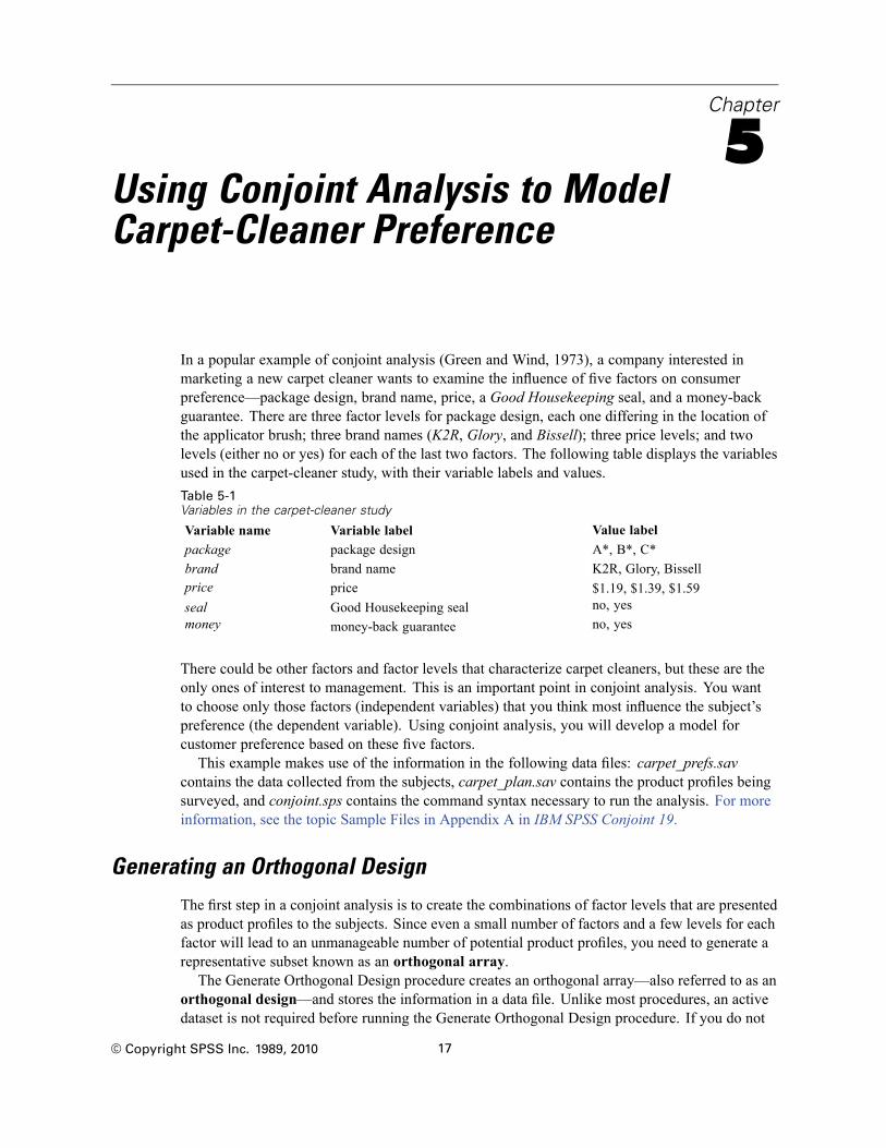
In a popular example of conjoint analysis (Green and Wind, 1973), a company interested in marketing a new carpet cleaner wants to examine the influence of five factors on consumer preference—package design, brand name, price, a Good Housekeeping seal, and a money-back guarantee. There are three factor levels for package design, each one differing in the location of the applicator brush; three brand names (K2R, Glory, and Bissell); three price levels; and two levels (either no or yes) for each of the last two factors. The following table displays the variables used in the carpet-cleaner study, with their variable labels and values. Table 5-1 Variables in the carpet-cleaner study
Variable name Variable label Value label package package design A*, B*, C* brand brand name K2R, Glory, Bissell price price $1.19, $1.39, $1.59 seal Good Housekeeping seal no, yes money money-back guarantee no, yes
There could be other factors and factor levels that characterize carpet cleaners, but these are the only ones of interest to management. This is an important point in conjoint analysis. You want to choose only those factors (independent variables) that you think most influence the subject’s preference (the dependent variable). Using conjoint analysis, you will develop a model for customer preference based on these five factors. This example makes use of the information in the following data files: carpet_prefs.sav
contains the data collected from the subjects, carpet_plan.sav contains the product profiles being surveyed, and conjoint.sps contains the command syntax necessary to run the analysis. For more information, see the topic Sample Files in Appendix A in IBM SPSS Conjoint 19.
Generating an Orthogonal Design
The first step in a conjoint analysis is to create the combinations of factor levels that are presented as product profiles to the subjects. Since even a small number of factors and a few levels for each factor will lead to an unmanageable number of potential product profiles, you need to generate a representative subset known as an orthogonal array. The Generate Orthogonal Design procedure creates an orthogonal array—also referred to as an
orthogonal design—and stores the information in a data file. Unlike most procedures, an active dataset is not required before running the Generate Orthogonal Design procedure. If you do not
© Copyright SPSS Inc. 1989, 2010 17
18
Chapter 5
have an active dataset, you have the option of creating one, generating variable names, variable labels, and value labels from the options that you select in the dialog boxes. If you already have an active dataset, you can either replace it or save the orthogonal design as a separate data file.
To create an orthogonal design:
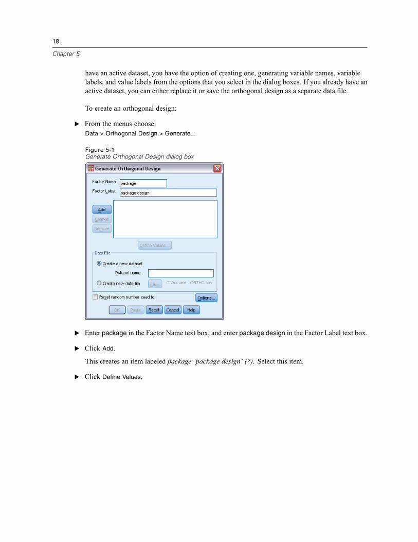
E From the menus choose: Data > Orthogonal Design > Generate...
Figure 5-1 Generate Orthogonal Design dialog box
E Enter package in the Factor Name text box, and enter package design in the Factor Label text box.
E Click Add.
This creates an item labeled package ‘package design’ (?). Select this item.
E Click Define Values.
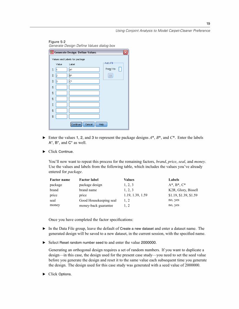
Figure 5-2 Generate Design Define Values dialog box
E Enter the values 1, 2, and 3 to represent the package designs A*, B*, and C*. Enter the labels A*, B*, and C* as well.
E Click Continue.
You’ll now want to repeat this process for the remaining factors, brand, price, seal, and money. Use the values and labels from the following table, which includes the values you’ve already entered for package.
Factor name Factor label Values Labels package package design 1, 2, 3 A*, B*, C* brand brand name 1, 2, 3 K2R, Glory, Bissell price price 1.19, 1.39, 1.59 $1.19, $1.39, $1.59 seal Good Housekeeping seal 1, 2 no, yes money money-back guarantee 1, 2 no, yes
Once you have completed the factor specifications:
E In the Data File group, leave the default of Create a new dataset and enter a dataset name. The generated design will be saved to a new dataset, in the current session, with the specified name.
E Select Reset random number seed to and enter the value 2000000.
Generating an orthogonal design requires a set of random numbers. If you want to duplicate a design—in this case, the design used for the present case study—you need to set the seed value before you generate the design and reset it to the same value each subsequent time you generate the design. The design used for this case study was generated with a seed value of 2000000.
E Click Options.
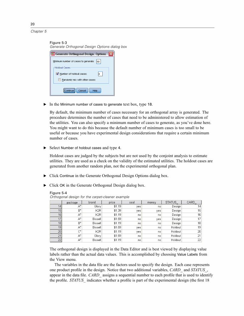
Figure 5-3 Generate Orthogonal Design Options dialog box
E In the Minimum number of cases to generate text box, type 18.
By default, the minimum number of cases necessary for an orthogonal array is generated. The procedure determines the number of cases that need to be administered to allow estimation of the utilities. You can also specify a minimum number of cases to generate, as you’ve done here. You might want to do this because the default number of minimum cases is too small to be useful or because you have experimental design considerations that require a certain minimum number of cases.
E Select Number of holdout cases and type 4.
Holdout cases are judged by the subjects but are not used by the conjoint analysis to estimate utilities. They are used as a check on the validity of the estimated utilities. The holdout cases are generated from another random plan, not the experimental orthogonal plan.
E Click Continue in the Generate Orthogonal Design Options dialog box.
E Click OK in the Generate Orthogonal Design dialog box.
Figure 5-4 Orthogonal design for the carpet-cleaner example
The orthogonal design is displayed in the Data Editor and is best viewed by displaying value labels rather than the actual data values. This is accomplished by choosing Value Labels from the View menu. The variables in the data file are the factors used to specify the design. Each case represents
one product profile in the design. Notice that two additional variables, CARD_ and STATUS_, appear in the data file. CARD_ assigns a sequential number to each profile that is used to identify the profile. STATUS_ indicates whether a profile is part of the experimental design (the first 18
21
Using Conjoint Analysis to Model Carpet-Cleaner Preference
cases), a holdout case (the last 4 cases), or a simulation case (to be discussed in a later topic in this case study). The orthogonal design is a required input to the analysis of the data. Therefore, you will
want to save your design to a data file. For convenience, the current design has been saved in carpet_plan.sav (orthogonal designs are also referred to as plans).
Creating the Experimental Stimuli: Displaying the Design
Once you have created an orthogonal design, you’ll want to use it to create the product profiles to be rated by the subjects. You can obtain a listing of the profiles in a single table or display each profile in a separate table.
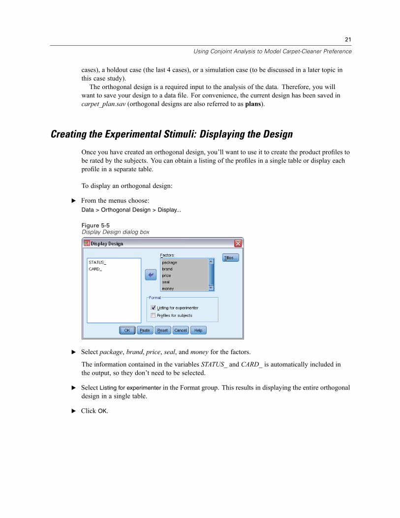
To display an orthogonal design:
E From the menus choose: Data > Orthogonal Design > Display...
Figure 5-5 Display Design dialog box
E Select package, brand, price, seal, and money for the factors.
The information contained in the variables STATUS_ and CARD_ is automatically included in the output, so they don’t need to be selected.
E Select Listing for experimenter in the Format group. This results in displaying the entire orthogonal design in a single table.
E Click OK.
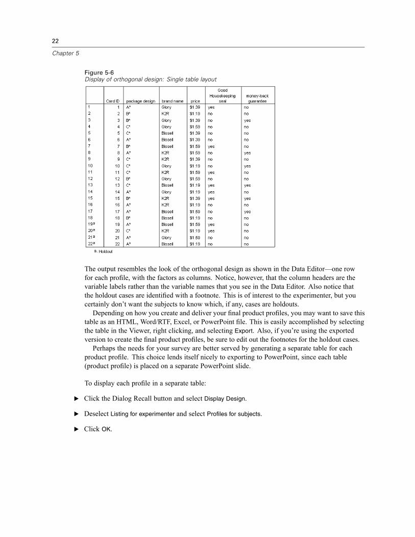
Figure 5-6 Display of orthogonal design: Single table layout
The output resembles the look of the orthogonal design as shown in the Data Editor—one row for each profile, with the factors as columns. Notice, however, that the column headers are the variable labels rather than the variable names that you see in the Data Editor. Also notice that the holdout cases are identified with a footnote. This is of interest to the experimenter, but you certainly don’t want the subjects to know which, if any, cases are holdouts. Depending on how you create and deliver your final product profiles, you may want to save this
table as an HTML, Word/RTF, Excel, or PowerPoint file. This is easily accomplished by selecting the table in the Viewer, right clicking, and selecting Export. Also, if you’re using the exported version to create the final product profiles, be sure to edit out the footnotes for the holdout cases. Perhaps the needs for your survey are better served by generating a separate table for each
product profile. This choice lends itself nicely to exporting to PowerPoint, since each table (product profile) is placed on a separate PowerPoint slide.
To display each profile in a separate table:
E Click the Dialog Recall button and select Display Design.
E Deselect Listing for experimenter and select Profiles for subjects.
E Click OK.
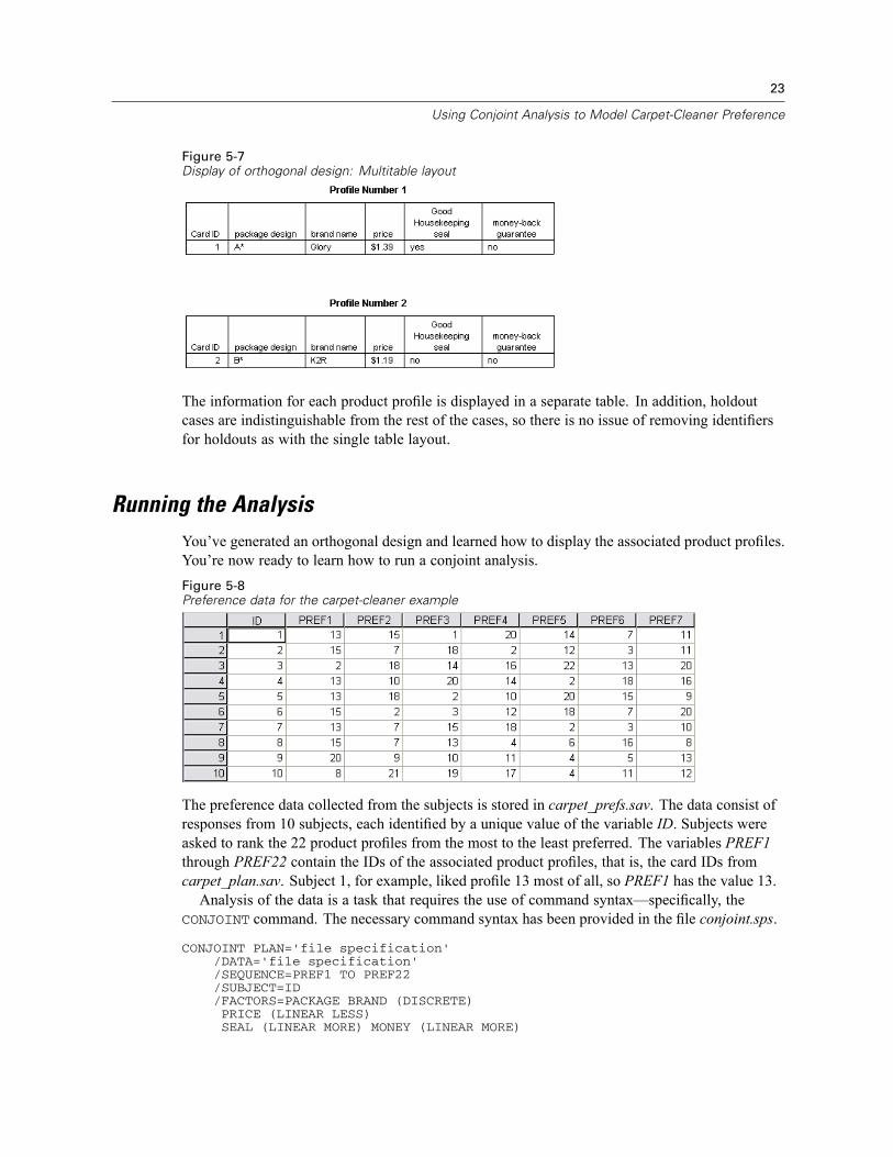
Figure 5-7 Display of orthogonal design: Multitable layout
The information for each product profile is displayed in a separate table. In addition, holdout cases are indistinguishable from the rest of the cases, so there is no issue of removing identifiers for holdouts as with the single table layout.
Running the Analysis You’ve generated an orthogonal design and learned how to display the associated product profiles. You’re now ready to learn how to run a conjoint analysis. Figure 5-8 Preference data for the carpet-cleaner example
The preference data collected from the subjects is stored in carpet_prefs.sav. The data consist of responses from 10 subjects, each identified by a unique value of the variable ID. Subjects were asked to rank the 22 product profiles from the most to the least preferred. The variables PREF1 through PREF22 contain the IDs of the associated product profiles, that is, the card IDs from carpet_plan.sav. Subject 1, for example, liked profile 13 most of all, so PREF1 has the value 13. Analysis of the data is a task that requires the use of command syntax—specifically, the
CONJOINT command. The necessary command syntax has been provided in the file conjoint.sps.
CONJOINT PLAN='file specification' /DATA='file specification' /SEQUENCE=PREF1 TO PREF22 /SUBJECT=ID /FACTORS=PACKAGE BRAND (DISCRETE) PRICE (LINEAR LESS) SEAL (LINEAR MORE) MONEY (LINEAR MORE)
24
Chapter 5
/PRINT=SUMMARYONLY.
The PLAN subcommand specifies the file containing the orthogonal design—in this example, carpet_plan.sav. The DATA subcommand specifies the file containing the preference data—in this example, carpet_prefs.sav. If you choose the preference data as the active dataset, you can replace the file specification with an asterisk (*), without the quotation marks. The SEQUENCE subcommand specifies that each data point in the preference data is a profile number, starting with the most-preferred profile and ending with the least-preferred profile. The SUBJECT subcommand specifies that the variable ID identifies the subjects. The FACTORS subcommand specifies a model describing the expected relationship between the preference data and the factor levels. The specified factors refer to variables defined in the plan file named on the PLAN subcommand. The keyword DISCRETE is used when the factor levels are categorical and no assumption is made about the relationship between the levels and the data. This is the case for the factors package and brand that represent package design and brand name, respectively. DISCRETE is assumed if a factor is not labeled with one of the four alternatives (DISCRETE, LINEAR, IDEAL, ANTIIDEAL) or is not included on the FACTORS subcommand. The keyword LINEAR, used for the remaining factors, indicates that the data are expected to be linearly related to the factor. For example, preference is usually expected to be linearly related to price. You can also specify quadratic models (not used in this example) with the keywords IDEAL and ANTIIDEAL. The keywords MORE and LESS, following LINEAR, indicate an expected direction for the relationship. Since we expect higher preference for lower prices, the keyword LESS is used for price. However, we expect higher preference for either a Good Housekeeping seal of approval or a money-back guarantee, so the keyword MORE is used for seal and money (recall that the levels for both of these factors were set to 1 for no and 2 for yes). Specifying MORE or LESS does not change the signs of the coefficients or affect estimates of the utilities. These keywords are used simply to identify subjects whose estimates do not match the expected direction. Similarly, choosing IDEAL instead of ANTIIDEAL, or vice versa, does not affect coefficients or utilities. The PRINT subcommand specifies that the output contains information for the group of subjects only as a whole (SUMMARYONLY keyword). Information for each subject, separately, is suppressed.
Try running this command syntax. Make sure that you have included valid paths to carpet_prefs.sav and carpet_plan.sav. For a complete description of all options, see the CONJOINT command in the Command Syntax Reference.
25
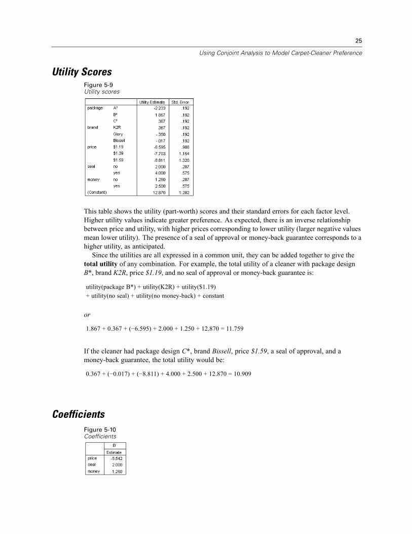
Utility Scores Figure 5-9 Utility scores
This table shows the utility (part-worth) scores and their standard errors for each factor level. Higher utility values indicate greater preference. As expected, there is an inverse relationship between price and utility, with higher prices corresponding to lower utility (larger negative values mean lower utility). The presence of a seal of approval or money-back guarantee corresponds to a higher utility, as anticipated. Since the utilities are all expressed in a common unit, they can be added together to give the
total utility of any combination. For example, the total utility of a cleaner with package design B*, brand K2R, price $1.19, and no seal of approval or money-back guarantee is:
utility(package B*) + utility(K2R) + utility($1.19) + utility(no seal) + utility(no money-back) + constant
or
1.867 + 0.367 + (−6.595) + 2.000 + 1.250 + 12.870 = 11.759
If the cleaner had package design C*, brand Bissell, price $1.59, a seal of approval, and a money-back guarantee, the total utility would be:
0.367 + (−0.017) + (−8.811) + 4.000 + 2.500 + 12.870 = 10.909
Coefficients Figure 5-10 Coefficients
Chapter 5
This table shows the linear regression coefficients for those factors specified as LINEAR (for IDEAL and ANTIIDEAL models, there would also be a quadratic term). The utility for a particular factor level is determined by multiplying the level by the coefficient. For example, the predicted utility for a price of $1.19 was listed as −6.595 in the utilities table. This is simply the value of the price level, 1.19, multiplied by the price coefficient, −5.542.
Relative Importance
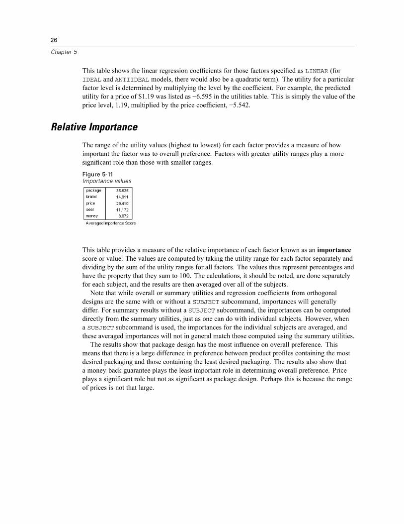
The range of the utility values (highest to lowest) for each factor provides a measure of how important the factor was to overall preference. Factors with greater utility ranges play a more significant role than those with smaller ranges.
Figure 5-11 Importance values
This table provides a measure of the relative importance of each factor known as an importance score or value. The values are computed by taking the utility range for each factor separately and dividing by the sum of the utility ranges for all factors. The values thus represent percentages and have the property that they sum to 100. The calculations, it should be noted, are done separately for each subject, and the results are then averaged over all of the subjects. Note that while overall or summary utilities and regression coefficients from orthogonal
designs are the same with or without a SUBJECT subcommand, importances will generally differ. For summary results without a SUBJECT subcommand, the importances can be computed directly from the summary utilities, just as one can do with individual subjects. However, when a SUBJECT subcommand is used, the importances for the individual subjects are averaged, and these averaged importances will not in general match those computed using the summary utilities. The results show that package design has the most influence on overall preference. This
means that there is a large difference in preference between product profiles containing the most desired packaging and those containing the least desired packaging. The results also show that a money-back guarantee plays the least important role in determining overall preference. Price plays a significant role but not as significant as package design. Perhaps this is because the range of prices is not that large.
27
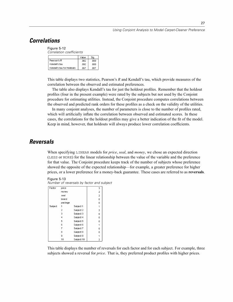
Correlations Figure 5-12 Correlation coefficients
This table displays two statistics, Pearson’s R and Kendall’s tau, which provide measures of the correlation between the observed and estimated preferences. The table also displays Kendall’s tau for just the holdout profiles. Remember that the holdout
profiles (four in the present example) were rated by the subjects but not used by the Conjoint procedure for estimating utilities. Instead, the Conjoint procedure computes correlations between the observed and predicted rank orders for these profiles as a check on the validity of the utilities. In many conjoint analyses, the number of parameters is close to the number of profiles rated,
which will artificially inflate the correlation between observed and estimated scores. In these cases, the correlations for the holdout profiles may give a better indication of the fit of the model. Keep in mind, however, that holdouts will always produce lower correlation coefficients.
Reversals
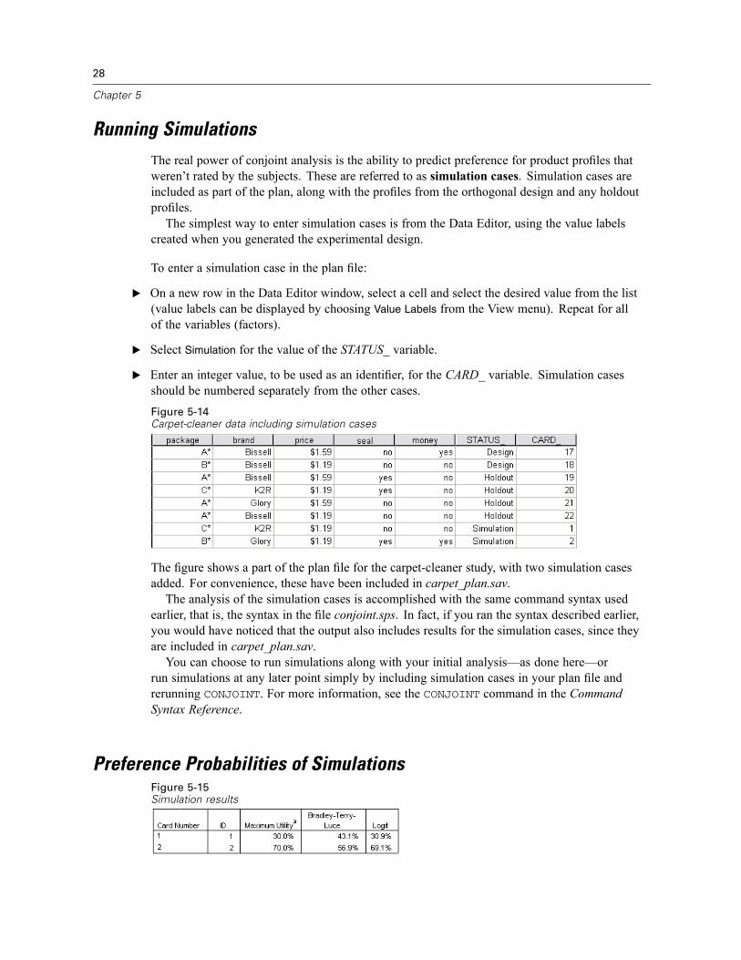
When specifying LINEAR models for price, seal, and money, we chose an expected direction (LESS or MORE) for the linear relationship between the value of the variable and the preference for that value. The Conjoint procedure keeps track of the number of subjects whose preference showed the opposite of the expected relationship—for example, a greater preference for higher prices, or a lower preference for a money-back guarantee. These cases are referred to as reversals.
Figure 5-13 Number of reversals by factor and subject
This table displays the number of reversals for each factor and for each subject. For example, three subjects showed a reversal for price. That is, they preferred product profiles with higher prices.
28
Chapter 5
Running Simulations The real power of conjoint analysis is the ability to predict preference for product profiles that weren’t rated by the subjects. These are referred to as simulation cases. Simulation cases are included as part of the plan, along with the profiles from the orthogonal design and any holdout profiles. The simplest way to enter simulation cases is from the Data Editor, using the value labels
created when you generated the experimental design.
To enter a simulation case in the plan file:
E On a new row in the Data Editor window, select a cell and select the desired value from the list (value labels can be displayed by choosing Value Labels from the View menu). Repeat for all of the variables (factors).
E Select Simulation for the value of the STATUS_ variable.
E Enter an integer value, to be used as an identifier, for the CARD_ variable. Simulation cases should be numbered separately from the other cases. Figure 5-14 Carpet-cleaner data including simulation cases
The figure shows a part of the plan file for the carpet-cleaner study, with two simulation cases added. For convenience, these have been included in carpet_plan.sav. The analysis of the simulation cases is accomplished with the same command syntax used
earlier, that is, the syntax in the file conjoint.sps. In fact, if you ran the syntax described earlier, you would have noticed that the output also includes results for the simulation cases, since they are included in carpet_plan.sav. You can choose to run simulations along with your initial analysis—as done here—or
run simulations at any later point simply by including simulation cases in your plan file and rerunning CONJOINT. For more information, see the CONJOINT command in the Command Syntax Reference.
Preference Probabilities of Simulations Figure 5-15 Simulation results
29
Using Conjoint Analysis to Model Carpet-Cleaner Preference
This table gives the predicted probabilities of choosing each of the simulation cases as the most preferred one, under three different probability-of-choice models. The maximum utility model determines the probability as the number of respondents predicted to choose the profile divided by the total number of respondents. For each respondent, the predicted choice is simply the profile with the largest total utility. The BTL (Bradley-Terry-Luce) model determines the probability as the ratio of a profile’s utility to that for all simulation profiles, averaged across all respondents. The logit model is similar to BTL but uses the natural log of the utilities instead of the utilities. Across the 10 subjects in this study, all three models indicated that simulation profile 2 would be preferred.
Appendix
A Sample Files
The sample files installed with the product can be found in the Samples subdirectory of the installation directory. There is a separate folder within the Samples subdirectory for each of the following languages: English, French, German, Italian, Japanese, Korean, Polish, Russian, Simplified Chinese, Spanish, and Traditional Chinese.
Not all sample files are available in all languages. If a sample file is not available in a language, that language folder contains an English version of the sample file.
Descriptions
Following are brief descriptions of the sample files used in various examples throughout the documentation.
accidents.sav. This is a hypothetical data file that concerns an insurance company that is studying age and gender risk factors for automobile accidents in a given region. Each case corresponds to a cross-classification of age category and gender. adl.sav. This is a hypothetical data file that concerns efforts to determine the benefits of a proposed type of therapy for stroke patients. Physicians randomly assigned female stroke patients to one of two groups. The first received the standard physical therapy, and the second received an additional emotional therapy. Three months following the treatments, each patient’s abilities to perform common activities of daily life were scored as ordinal variables. advert.sav. This is a hypothetical data file that concerns a retailer’s efforts to examine the relationship between money spent on advertising and the resulting sales. To this end, they have collected past sales figures and the associated advertising costs.. aflatoxin.sav. This is a hypothetical data file that concerns the testing of corn crops for aflatoxin, a poison whose concentration varies widely between and within crop yields. A grain processor has received 16 samples from each of 8 crop yields and measured the alfatoxin levels in parts per billion (PPB). anorectic.sav. While working toward a standardized symptomatology of anorectic/bulimic behavior, researchers (Van der Ham, Meulman, Van Strien, and Van Engeland, 1997) made a study of 55 adolescents with known eating disorders. Each patient was seen four times over four years, for a total of 220 observations. At each observation, the patients were scored for each of 16 symptoms. Symptom scores are missing for patient 71 at time 2, patient 76 at time 2, and patient 47 at time 3, leaving 217 valid observations. bankloan.sav. This is a hypothetical data file that concerns a bank’s efforts to reduce the rate of loan defaults. The file contains financial and demographic information on 850 past and prospective customers. The first 700 cases are customers who were previously given
© Copyright SPSS Inc. 1989, 2010 30
31
Sample Files
loans. The last 150 cases are prospective customers that the bank needs to classify as good or bad credit risks. bankloan_binning.sav. This is a hypothetical data file containing financial and demographic information on 5,000 past customers. behavior.sav. In a classic example (Price and Bouffard, 1974), 52 students were asked to rate the combinations of 15 situations and 15 behaviors on a 10-point scale ranging from 0=“extremely appropriate” to 9=“extremely inappropriate.” Averaged over individuals, the values are taken as dissimilarities. behavior_ini.sav. This data file contains an initial configuration for a two-dimensional solution for behavior.sav. brakes.sav. This is a hypothetical data file that concerns quality control at a factory that produces disc brakes for high-performance automobiles. The data file contains diameter measurements of 16 discs from each of 8 production machines. The target diameter for the brakes is 322 millimeters. breakfast.sav. In a classic study (Green and Rao, 1972), 21 Wharton School MBA students and their spouses were asked to rank 15 breakfast items in order of preference with 1=“most preferred” to 15=“least preferred.” Their preferences were recorded under six different scenarios, from “Overall preference” to “Snack, with beverage only.” breakfast-overall.sav. This data file contains the breakfast item preferences for the first scenario, “Overall preference,” only. broadband_1.sav. This is a hypothetical data file containing the number of subscribers, by region, to a national broadband service. The data file contains monthly subscriber numbers for 85 regions over a four-year period. broadband_2.sav. This data file is identical to broadband_1.sav but contains data for three additional months. car_insurance_claims.sav. A dataset presented and analyzed elsewhere (McCullagh and Nelder, 1989) concerns damage claims for cars. The average claim amount can be modeled as having a gamma distribution, using an inverse link function to relate the mean of the dependent variable to a linear combination of the policyholder age, vehicle type, and vehicle age. The number of claims filed can be used as a scaling weight. car_sales.sav. This data file contains hypothetical sales estimates, list prices, and physical specifications for various makes and models of vehicles. The list prices and physical specifications were obtained alternately from edmunds.com and manufacturer sites. car_sales_uprepared.sav. This is a modified version of car_sales.sav that does not include any transformed versions of the fields. carpet.sav. In a popular example (Green and Wind, 1973), a company interested in marketing a new carpet cleaner wants to examine the influence of five factors on consumer preference—package design, brand name, price, a Good Housekeeping seal, and a money-back guarantee. There are three factor levels for package design, each one differing in the location of the applicator brush; three brand names (K2R, Glory, and Bissell); three price levels; and two levels (either no or yes) for each of the last two factors. Ten consumers rank 22 profiles defined by these factors. The variable Preference contains the rank of the average rankings for each profile. Low rankings correspond to high preference. This variable reflects an overall measure of preference for each profile.
32
Appendix A
carpet_prefs.sav. This data file is based on the same example as described for carpet.sav, but it contains the actual rankings collected from each of the 10 consumers. The consumers were asked to rank the 22 product profiles from the most to the least preferred. The variables PREF1 through PREF22 contain the identifiers of the associated profiles, as defined in carpet_plan.sav. catalog.sav. This data file contains hypothetical monthly sales figures for three products sold by a catalog company. Data for five possible predictor variables are also included. catalog_seasfac.sav. This data file is the same as catalog.sav except for the addition of a set of seasonal factors calculated from the Seasonal Decomposition procedure along with the accompanying date variables. cellular.sav. This is a hypothetical data file that concerns a cellular phone company’s efforts to reduce churn. Churn propensity scores are applied to accounts, ranging from 0 to 100. Accounts scoring 50 or above may be looking to change providers. ceramics.sav. This is a hypothetical data file that concerns a manufacturer’s efforts to determine whether a new premium alloy has a greater heat resistance than a standard alloy. Each case represents a separate test of one of the alloys; the heat at which the bearing failed is recorded. cereal.sav. This is a hypothetical data file that concerns a poll of 880 people about their breakfast preferences, also noting their age, gender, marital status, and whether or not they have an active lifestyle (based on whether they exercise at least twice a week). Each case represents a separate respondent. clothing_defects.sav. This is a hypothetical data file that concerns the quality control process at a clothing factory. From each lot produced at the factory, the inspectors take a sample of clothes and count the number of clothes that are unacceptable. coffee.sav. This data file pertains to perceived images of six iced-coffee brands (Kennedy, Riquier, and Sharp, 1996) . For each of 23 iced-coffee image attributes, people selected all brands that were described by the attribute. The six brands are denoted AA, BB, CC, DD, EE, and FF to preserve confidentiality. contacts.sav. This is a hypothetical data file that concerns the contact lists for a group of corporate computer sales representatives. Each contact is categorized by the department of the company in which they work and their company ranks. Also recorded are the amount of the last sale made, the time since the last sale, and the size of the contact’s company. creditpromo.sav. This is a hypothetical data file that concerns a department store’s efforts to evaluate the effectiveness of a recent credit card promotion. To this end, 500 cardholders were randomly selected. Half received an ad promoting a reduced interest rate on purchases made over the next three months. Half received a standard seasonal ad. customer_dbase.sav. This is a hypothetical data file that concerns a company’s efforts to use the information in its data warehouse to make special offers to customers who are most likely to reply. A subset of the customer base was selected at random and given the special offers, and their responses were recorded. customer_information.sav. A hypothetical data file containing customer mailing information, such as name and address. customer_subset.sav. A subset of 80 cases from customer_dbase.sav.
33
Sample Files
debate.sav. This is a hypothetical data file that concerns paired responses to a survey from attendees of a political debate before and after the debate. Each case corresponds to a separate respondent. debate_aggregate.sav. This is a hypothetical data file that aggregates the responses in debate.sav. Each case corresponds to a cross-classification of preference before and after the debate. demo.sav. This is a hypothetical data file that concerns a purchased customer database, for the purpose of mailing monthly offers. Whether or not the customer responded to the offer is recorded, along with various demographic information. demo_cs_1.sav. This is a hypothetical data file that concerns the first step of a company’s efforts to compile a database of survey information. Each case corresponds to a different city, and the region, province, district, and city identification are recorded. demo_cs_2.sav. This is a hypothetical data file that concerns the second step of a company’s efforts to compile a database of survey information. Each case corresponds to a different household unit from cities selected in the first step, and the region, province, district, city, subdivision, and unit identification are recorded. The sampling information from the first two stages of the design is also included. demo_cs.sav. This is a hypothetical data file that contains survey information collected using a complex sampling design. Each case corresponds to a different household unit, and various demographic and sampling information is recorded. dmdata.sav. This is a hypothetical data file that contains demographic and purchasing information for a direct marketing company. dmdata2.sav contains information for a subset of contacts that received a test mailing, and dmdata3.sav contains information on the remaining contacts who did not receive the test mailing. dietstudy.sav. This hypothetical data file contains the results of a study of the “Stillman diet” (Rickman, Mitchell, Dingman, and Dalen, 1974). Each case corresponds to a separate subject and records his or her pre- and post-diet weights in pounds and triglyceride levels in mg/100 ml. dvdplayer.sav. This is a hypothetical data file that concerns the development of a new DVD player. Using a prototype, the marketing team has collected focus group data. Each case corresponds to a separate surveyed user and records some demographic information about them and their responses to questions about the prototype. german_credit.sav. This data file is taken from the “German credit” dataset in the Repository of Machine Learning Databases (Blake and Merz, 1998) at the University of California, Irvine. grocery_1month.sav. This hypothetical data file is the grocery_coupons.sav data file with the weekly purchases “rolled-up” so that each case corresponds to a separate customer. Some of the variables that changed weekly disappear as a result, and the amount spent recorded is now the sum of the amounts spent during the four weeks of the study. grocery_coupons.sav. This is a hypothetical data file that contains survey data collected by a grocery store chain interested in the purchasing habits of their customers. Each customer is followed for four weeks, and each case corresponds to a separate customer-week and records information about where and how the customer shops, including how much was spent on groceries during that week.
34
Appendix A
guttman.sav. Bell (Bell, 1961) presented a table to illustrate possible social groups. Guttman (Guttman, 1968) used a portion of this table, in which five variables describing such things as social interaction, feelings of belonging to a group, physical proximity of members, and formality of the relationship were crossed with seven theoretical social groups, including crowds (for example, people at a football game), audiences (for example, people at a theater or classroom lecture), public (for example, newspaper or television audiences), mobs (like a crowd but with much more intense interaction), primary groups (intimate), secondary groups (voluntary), and the modern community (loose confederation resulting from close physical proximity and a need for specialized services). health_funding.sav. This is a hypothetical data file that contains data on health care funding (amount per 100 population), disease rates (rate per 10,000 population), and visits to health care providers (rate per 10,000 population). Each case represents a different city. hivassay.sav. This is a hypothetical data file that concerns the efforts of a pharmaceutical lab to develop a rapid assay for detecting HIV infection. The results of the assay are eight deepening shades of red, with deeper shades indicating greater likelihood of infection. A laboratory trial was conducted on 2,000 blood samples, half of which were infected with HIV and half of which were clean. hourlywagedata.sav. This is a hypothetical data file that concerns the hourly wages of nurses from office and hospital positions and with varying levels of experience. insurance_claims.sav. This is a hypothetical data file that concerns an insurance company that wants to build a model for flagging suspicious, potentially fraudulent claims. Each case represents a separate claim. insure.sav. This is a hypothetical data file that concerns an insurance company that is studying the risk factors that indicate whether a client will have to make a claim on a 10-year term life insurance contract. Each case in the data file represents a pair of contracts, one of which recorded a claim and the other didn’t, matched on age and gender. judges.sav. This is a hypothetical data file that concerns the scores given by trained judges (plus one enthusiast) to 300 gymnastics performances. Each row represents a separate performance; the judges viewed the same performances. kinship_dat.sav. Rosenberg and Kim (Rosenberg and Kim, 1975) set out to analyze 15 kinship terms (aunt, brother, cousin, daughter, father, granddaughter, grandfather, grandmother, grandson, mother, nephew, niece, sister, son, uncle). They asked four groups of college students (two female, two male) to sort these terms on the basis of similarities. Two groups (one female, one male) were asked to sort twice, with the second sorting based on a different criterion from the first sort. Thus, a total of six “sources” were obtained. Each source corresponds to a proximity matrix, whose cells are equal to the number of people in a source minus the number of times the objects were partitioned together in that source. kinship_ini.sav. This data file contains an initial configuration for a three-dimensional solution for kinship_dat.sav. kinship_var.sav. This data file contains independent variables gender, gener(ation), and degree (of separation) that can be used to interpret the dimensions of a solution for kinship_dat.sav. Specifically, they can be used to restrict the space of the solution to a linear combination of these variables. marketvalues.sav. This data file concerns home sales in a new housing development in Algonquin, Ill., during the years from 1999–2000. These sales are a matter of public record.
35
Sample Files
nhis2000_subset.sav. The National Health Interview Survey (NHIS) is a large, population-based survey of the U.S. civilian population. Interviews are carried out face-to-face in a nationally representative sample of households. Demographic information and observations about health behaviors and status are obtained for members of each household. This data file contains a subset of information from the 2000 survey. National Center for Health Statistics. National Health Interview Survey, 2000. Public-use data file and documentation. ftp://ftp.cdc.gov/pub/Health_Statistics/NCHS/Datasets/NHIS/2000/. Accessed 2003. ozone.sav. The data include 330 observations on six meteorological variables for predicting ozone concentration from the remaining variables. Previous researchers (Breiman and Friedman, 1985), (Hastie and Tibshirani, 1990), among others found nonlinearities among these variables, which hinder standard regression approaches. pain_medication.sav. This hypothetical data file contains the results of a clinical trial for anti-inflammatory medication for treating chronic arthritic pain. Of particular interest is the time it takes for the drug to take effect and how it compares to an existing medication. patient_los.sav. This hypothetical data file contains the treatment records of patients who were admitted to the hospital for suspected myocardial infarction (MI, or “heart attack”). Each case corresponds to a separate patient and records many variables related to their hospital stay. patlos_sample.sav. This hypothetical data file contains the treatment records of a sample of patients who received thrombolytics during treatment for myocardial infarction (MI, or “heart attack”). Each case corresponds to a separate patient and records many variables related to their hospital stay. poll_cs.sav. This is a hypothetical data file that concerns pollsters’ efforts to determine the level of public support for a bill before the legislature. The cases correspond to registered voters. Each case records the county, township, and neighborhood in which the voter lives. poll_cs_sample.sav. This hypothetical data file contains a sample of the voters listed in poll_cs.sav. The sample was taken according to the design specified in the poll.csplan plan file, and this data file records the inclusion probabilities and sample weights. Note, however, that because the sampling plan makes use of a probability-proportional-to-size (PPS) method, there is also a file containing the joint selection probabilities (poll_jointprob.sav). The additional variables corresponding to voter demographics and their opinion on the proposed bill were collected and added the data file after the sample as taken. property_assess.sav. This is a hypothetical data file that concerns a county assessor’s efforts to keep property value assessments up to date on limited resources. The cases correspond to properties sold in the county in the past year. Each case in the data file records the township in which the property lies, the assessor who last visited the property, the time since that assessment, the valuation made at that time, and the sale value of the property. property_assess_cs.sav. This is a hypothetical data file that concerns a state assessor’s efforts to keep property value assessments up to date on limited resources. The cases correspond to properties in the state. Each case in the data file records the county, township, and neighborhood in which the property lies, the time since the last assessment, and the valuation made at that time. property_assess_cs_sample.sav. This hypothetical data file contains a sample of the properties listed in property_assess_cs.sav. The sample was taken according to the design specified in the property_assess.csplan plan file, and this data file records the inclusion probabilities
36
Appendix A
and sample weights. The additional variable Current value was collected and added to the data file after the sample was taken. recidivism.sav. This is a hypothetical data file that concerns a government law enforcement agency’s efforts to understand recidivism rates in their area of jurisdiction. Each case corresponds to a previous offender and records their demographic information, some details of their first crime, and then the time until their second arrest, if it occurred within two years of the first arrest. recidivism_cs_sample.sav. This is a hypothetical data file that concerns a government law enforcement agency’s efforts to understand recidivism rates in their area of jurisdiction. Each case corresponds to a previous offender, released from their first arrest during the month of June, 2003, and records their demographic information, some details of their first crime, and the data of their second arrest, if it occurred by the end of June, 2006. Offenders were selected from sampled departments according to the sampling plan specified in recidivism_cs.csplan; because it makes use of a probability-proportional-to-size (PPS) method, there is also a file containing the joint selection probabilities (recidivism_cs_jointprob.sav). rfm_transactions.sav. A hypothetical data file containing purchase transaction data, including date of purchase, item(s) purchased, and monetary amount of each transaction. salesperformance.sav. This is a hypothetical data file that concerns the evaluation of two new sales training courses. Sixty employees, divided into three groups, all receive standard training. In addition, group 2 gets technical training; group 3, a hands-on tutorial. Each employee was tested at the end of the training course and their score recorded. Each case in the data file represents a separate trainee and records the group to which they were assigned and the score they received on the exam. satisf.sav. This is a hypothetical data file that concerns a satisfaction survey conducted by a retail company at 4 store locations. 582 customers were surveyed in all, and each case represents the responses from a single customer. screws.sav. This data file contains information on the characteristics of screws, bolts, nuts, and tacks (Hartigan, 1975). shampoo_ph.sav. This is a hypothetical data file that concerns the quality control at a factory for hair products. At regular time intervals, six separate output batches are measured and their pH recorded. The target range is 4.5–5.5. ships.sav. A dataset presented and analyzed elsewhere (McCullagh et al., 1989) that concerns damage to cargo ships caused by waves. The incident counts can be modeled as occurring at a Poisson rate given the ship type, construction period, and service period. The aggregate months of service for each cell of the table formed by the cross-classification of factors provides values for the exposure to risk. site.sav. This is a hypothetical data file that concerns a company’s efforts to choose new sites for their expanding business. They have hired two consultants to separately evaluate the sites, who, in addition to an extended report, summarized each site as a “good,” “fair,” or “poor” prospect. smokers.sav. This data file is abstracted from the 1998 National Household Survey of Drug Abuse and is a probability sample of American households. (http://dx.doi.org/10.3886/ICPSR02934) Thus, the first step in an analysis of this data file should be to weight the data to reflect population trends.
Sample Files
stroke_clean.sav. This hypothetical data file contains the state of a medical database after it has been cleaned using procedures in the Data Preparation option. stroke_invalid.sav. This hypothetical data file contains the initial state of a medical database and contains several data entry errors. stroke_survival. This hypothetical data file concerns survival times for patients exiting a rehabilitation program post-ischemic stroke face a number of challenges. Post-stroke, the occurrence of myocardial infarction, ischemic stroke, or hemorrhagic stroke is noted and the time of the event recorded. The sample is left-truncated because it only includes patients who survived through the end of the rehabilitation program administered post-stroke. stroke_valid.sav. This hypothetical data file contains the state of a medical database after the values have been checked using the Validate Data procedure. It still contains potentially anomalous cases. survey_sample.sav. This data file contains survey data, including demographic data and various attitude measures. It is based on a subset of variables from the 1998 NORC General Social Survey, although some data values have been modified and additional fictitious variables have been added for demonstration purposes. telco.sav. This is a hypothetical data file that concerns a telecommunications company’s efforts to reduce churn in their customer base. Each case corresponds to a separate customer and records various demographic and service usage information. telco_extra.sav. This data file is similar to the telco.sav data file, but the “tenure” and log-transformed customer spending variables have been removed and replaced by standardized log-transformed customer spending variables. telco_missing.sav. This data file is a subset of the telco.sav data file, but some of the demographic data values have been replaced with missing values. testmarket.sav. This hypothetical data file concerns a fast food chain’s plans to add a new item to its menu. There are three possible campaigns for promoting the new product, so the new item is introduced at locations in several randomly selected markets. A different promotion is used at each location, and the weekly sales of the new item are recorded for the first four weeks. Each case corresponds to a separate location-week. testmarket_1month.sav. This hypothetical data file is the testmarket.sav data file with the weekly sales “rolled-up” so that each case corresponds to a separate location. Some of the variables that changed weekly disappear as a result, and the sales recorded is now the sum of the sales during the four weeks of the study. tree_car.sav. This is a hypothetical data file containing demographic and vehicle purchase price data. tree_credit.sav. This is a hypothetical data file containing demographic and bank loan history data. tree_missing_data.sav This is a hypothetical data file containing demographic and bank loan history data with a large number of missing values. tree_score_car.sav. This is a hypothetical data file containing demographic and vehicle purchase price data. tree_textdata.sav. A simple data file with only two variables intended primarily to show the default state of variables prior to assignment of measurement level and value labels.
38
Appendix A
tv-survey.sav. This is a hypothetical data file that concerns a survey conducted by a TV studio that is considering whether to extend the run of a successful program. 906 respondents were asked whether they would watch the program under various conditions. Each row represents a separate respondent; each column is a separate condition. ulcer_recurrence.sav. This file contains partial information from a study designed to compare the efficacy of two therapies for preventing the recurrence of ulcers. It provides a good example of interval-censored data and has been presented and analyzed elsewhere (Collett, 2003). ulcer_recurrence_recoded.sav. This file reorganizes the information in ulcer_recurrence.sav to allow you model the event probability for each interval of the study rather than simply the end-of-study event probability. It has been presented and analyzed elsewhere (Collett et al., 2003). verd1985.sav. This data file concerns a survey (Verdegaal, 1985). The responses of 15 subjects to 8 variables were recorded. The variables of interest are divided into three sets. Set 1 includes age and marital, set 2 includes pet and news, and set 3 includes music and live. Pet is scaled as multiple nominal and age is scaled as ordinal; all of the other variables are scaled as single nominal. virus.sav. This is a hypothetical data file that concerns the efforts of an Internet service provider (ISP) to determine the effects of a virus on its networks. They have tracked the (approximate) percentage of infected e-mail traffic on its networks over time, from the moment of discovery until the threat was contained. wheeze_steubenville.sav. This is a subset from a longitudinal study of the health effects of air pollution on children (Ware, Dockery, Spiro III, Speizer, and Ferris Jr., 1984). The data contain repeated binary measures of the wheezing status for children from Steubenville, Ohio, at ages 7, 8, 9 and 10 years, along with a fixed recording of whether or not the mother was a smoker during the first year of the study. workprog.sav. This is a hypothetical data file that concerns a government works program that tries to place disadvantaged people into better jobs. A sample of potential program participants were followed, some of whom were randomly selected for enrollment in the program, while others were not. Each case represents a separate program participant.
Appendix
B Notices
Licensed Materials – Property of SPSS Inc., an IBM Company. © Copyright SPSS Inc. 1989, 2010.
Patent No. 7,023,453
The following paragraph does not apply to the United Kingdom or any other country where such provisions are inconsistent with local law: SPSS INC., AN IBM COMPANY, PROVIDES THIS PUBLICATION “AS IS” WITHOUT WARRANTY OF ANY KIND, EITHER EXPRESS OR IMPLIED, INCLUDING, BUT NOT LIMITED TO, THE IMPLIED WARRANTIES OF NON-INFRINGEMENT, MERCHANTABILITY OR FITNESS FOR A PARTICULAR PURPOSE. Some states do not allow disclaimer of express or implied warranties in certain transactions, therefore, this statement may not apply to you.
This information could include technical inaccuracies or typographical errors. Changes are periodically made to the information herein; these changes will be incorporated in new editions of the publication. SPSS Inc. may make improvements and/or changes in the product(s) and/or the program(s) described in this publication at any time without notice.
Any references in this information to non-SPSS and non-IBM Web sites are provided for convenience only and do not in any manner serve as an endorsement of those Web sites. The materials at those Web sites are not part of the materials for this SPSS Inc. product and use of those Web sites is at your own risk.
When you send information to IBM or SPSS, you grant IBM and SPSS a nonexclusive right to use or distribute the information in any way it believes appropriate without incurring any obligation to you.
Information concerning non-SPSS products was obtained from the suppliers of those products, their published announcements or other publicly available sources. SPSS has not tested those products and cannot confirm the accuracy of performance, compatibility or any other claims related to non-SPSS products. Questions on the capabilities of non-SPSS products should be addressed to the suppliers of those products.
This information contains examples of data and reports used in daily business operations. To illustrate them as completely as possible, the examples include the names of individuals, companies, brands, and products. All of these names are fictitious and any similarity to the names and addresses used by an actual business enterprise is entirely coincidental.
COPYRIGHT LICENSE:
This information contains sample application programs in source language, which illustrate programming techniques on various operating platforms. You may copy, modify, and distribute these sample programs in any form without payment to SPSS Inc., for the purposes of developing,
© Copyright SPSS Inc. 1989, 2010 39
40
Appendix B
using, marketing or distributing application programs conforming to the application programming interface for the operating platform for which the sample programs are written. These examples have not been thoroughly tested under all conditions. SPSS Inc., therefore, cannot guarantee or imply reliability, serviceability, or function of these programs. The sample programs are provided “AS IS”, without warranty of any kind. SPSS Inc. shall not be liable for any damages arising out of your use of the sample programs.
Trademarks
IBM, the IBM logo, and ibm.com are trademarks of IBM Corporation, registered in many jurisdictions worldwide. A current list of IBM trademarks is available on the Web at http://www.ibm.com/legal/copytrade.shmtl.
SPSS is a trademark of SPSS Inc., an IBM Company, registered in many jurisdictions worldwide.
Adobe, the Adobe logo, PostScript, and the PostScript logo are either registered trademarks or trademarks of Adobe Systems Incorporated in the United States, and/or other countries.
Intel, Intel logo, Intel Inside, Intel Inside logo, Intel Centrino, Intel Centrino logo, Celeron, Intel Xeon, Intel SpeedStep, Itanium, and Pentium are trademarks or registered trademarks of Intel Corporation or its subsidiaries in the United States and other countries.
Linux is a registered trademark of Linus Torvalds in the United States, other countries, or both.
Microsoft, Windows, Windows NT, and the Windows logo are trademarks of Microsoft Corporation in the United States, other countries, or both.
UNIX is a registered trademark of The Open Group in the United States and other countries.
Java and all Java-based trademarks and logos are trademarks of Sun Microsystems, Inc. in the United States, other countries, or both.
This product uses WinWr

Bibliography

Akaah, I. P., and P. K. Korgaonkar. 1988. A conjoint investigation of the relative importance ofrisk relievers in direct marketing. Journal of Advertising Research, 28:4, 38–44.
Bell, E. H. 1961. Social foundations of human behavior: Introduction to the study of sociology.New York: Harper & Row.
Blake, C. L., and C. J. Merz. 1998. "UCI Repository of machine learning databases." Available athttp://www.ics.uci.edu/~mlearn/MLRepository.html.
Breiman, L., and J. H. Friedman. 1985. Estimating optimal transformations for multipleregression and correlation. Journal of the American Statistical Association, 80, 580–598.
Cattin, P., and D. R. Wittink. 1982. Commercial use of conjoint analysis: A survey. Journalof Marketing, 46:3, 44–53.
Collett, D. 2003. Modelling survival data in medical research, 2 ed. Boca Raton: Chapman &Hall/CRC.
Green, P. E., and V. Rao. 1972. Applied multidimensional scaling. Hinsdale, Ill.: Dryden Press.
Green, P. E., and Y. Wind. 1973. Multiattribute decisions in marketing: A measurement approach.Hinsdale, Ill.: Dryden Press.
Guttman, L. 1968. A general nonmetric technique for finding the smallest coordinate space forconfigurations of points. Psychometrika, 33, 469–506.
Hartigan, J. A. 1975. Clustering algorithms. New York: John Wiley and Sons.
Hastie, T., and R. Tibshirani. 1990. Generalized additive models. London: Chapman and Hall.
Kennedy, R., C. Riquier, and B. Sharp. 1996. Practical applications of correspondence analysisto categorical data in market research. Journal of Targeting, Measurement, and Analysis forMarketing, 5, 56–70.
McCullagh, P., and J. A. Nelder. 1989. Generalized Linear Models, 2nd ed. London: Chapman &Hall.
Price, R. H., and D. L. Bouffard. 1974. Behavioral appropriateness and situational constraints asdimensions of social behavior. Journal of Personality and Social Psychology, 30, 579–586.
Rickman, R., N. Mitchell, J. Dingman, and J. E. Dalen. 1974. Changes in serum cholesterolduring the Stillman Diet. Journal of the American Medical Association, 228, 54–58.
Rosenberg, S., and M. P. Kim. 1975. The method of sorting as a data-gathering procedure inmultivariate research. Multivariate Behavioral Research, 10, 489–502.
Van der Ham, T., J. J. Meulman, D. C. Van Strien, and H. Van Engeland. 1997. Empirically basedsubgrouping of eating disorders in adolescents: A longitudinal perspective. British Journal ofPsychiatry, 170, 363–368.
Verdegaal, R. 1985. Meer sets analyse voor kwalitatieve gegevens (in Dutch). Leiden: Departmentof Data Theory, University of Leiden.
© Copyright SPSS Inc. 1989, 2010 41
42
Ware, J. H., D. W. Dockery, A. Spiro III, F. E. Speizer, and B. G. Ferris Jr.. 1984. Passivesmoking, gas cooking, and respiratory health of children living in six cities. American Review ofRespiratory Diseases, 129, 366–374.
Index
anti-ideal model, 24
BTL (Bradley-Terry-Luce) model, 28
)CARDin Display Design, 10
card_ variablein Generate Orthogonal Design, 5
coefficients, 25command syntaxCONJOINT command, 23
correlation coefficients, 27
data filesin Generate Orthogonal Design, 5
discrete model, 24Display Design, 2, 9, 21)CARD, 10footers, 10listing format, 9saving profiles, 10single-profile format, 9titles, 10
factor levels, 2, 17factors, 2, 17footersin Display Design, 10
full-profile approach, 2
Generate Orthogonal Design, 2, 5, 17data files, 5defining factor names, labels, and values, 6holdout cases, 7minimum cases, 7random number seed, 5simulation cases, 8
holdout cases, 2in Generate Orthogonal Design, 7
ideal model, 24importance scores, 26importance values, 26
Kendall’s tau, 27
legal notices, 39
linear model, 24listing formatin Display Design, 9
logit model, 28
max utility model, 28
orthogonal array, 2orthogonal designsdisplaying, 9, 21generating, 5, 17holdout cases, 7minimum cases, 7
part-worths, 3Pearson’s R, 27
random number seedin Generate Orthogonal Design, 5
reversals, 27
sample fileslocation, 30
sample size, 2simulation cases, 3, 14, 28in Generate Orthogonal Design, 8
simulation resultsBTL (Bradley-Terry-Luce) model, 28logit model, 28max utility model, 28
single-profile formatin Display Design, 9
status_ variablein Generate Orthogonal Design, 5
syntaxCONJOINT command, 23
titlesin Display Design, 10
total utility, 25trademarks, 40
utility scores, 3, 25