


Languages
Pages
Legal

hydraulic performance of
controlled irrigation canals
Wytze Schuurmans
MODIS
User 's Guide
Appendix G of
A model to study
tfie hydraulic performance
of controlled irrigation canals
W y t z e S c h u u r m a n s
C o p y r i g h t ® b y C e n t r e f o r O p e r a t i o n a l W a t e r m a n a g e m e n t , D e l f t U n i v e r s i t y
o f T e c h n o l o g y , P.O. B o x 5 0 4 8 , 2 6 0 0 G A , D e l f t , T h e N e t h e r l a n d s .

i i

Preface
The MODIS model i s a computer program package which can be used to study
the h y d r a u l i c performance of c o n t r o l l e d c a n a l s . MODIS i s an acronym of
Modelling Drainage and I r r i g a t i o n systems, and has been developed out of
the e x i s t i n g program RUBICON developed f o r r i v e r a p p l i c a t i o n s .
The u s e r ' s guide c o n s i s t of t h r e e p a r t s . The f i r s t four c h a p t e r s provide
g e n e r a l information about the program package and i t s use. The second
p a r t ( c h a p t e r 5 to 10) d e a l s w i t h the input f i l e s of the program package.
I n an example a l l input f i l e s f o r a p a r t i c u l a r c ase a re worked out. The
t h i r d and l a s t p a r t of the u s e r ' s guide ( c h a p t e r 11 and 12) c o n t a i n s some
d e t a i l e d information about the mathematics u n d e r l y i n g the program and the
a p p l i e d numerical methods of s o l u t i o n .
I n a d d i t i o n to the u s e r ' s guide, a software documentation of the program
package i s a v a i l a b l e for those who a r e going to make model m o d i f i c a t i o n s .
Wytze Schuurmans, August 1991
i i i

i v
able of contents
Description of program M O D I S
1.1 I n t r o d u c t i o n 1-1
1.2 T e c h n i c a l m e r i t 1-2
1.3 Modeling c a p a b i l i t i e s 1-4
1.4 User c o n s i d e r a t i o n s 1-7
1.5 Summary and c o n c l u s i o n s 1-10
Getting started
2.1 s t r u c t u r e of the modis program package 2-1
2.2 I n s t a l l a t i o n of the program package 2-2
2.3 S t a r t i n g the program 2-3
2.4 How to use the operation template ? 2-4
2.4 Running the model 2-5
Modelling the watermanagement system
3.1 I n t r o d u c t i o n 3-1
3.2 The c a n a l system 3-1
3.3 Regulators 3-4
3.4 Con t r o l of r e g u l a t o r s 3-5
3.5 Operation performance c r i t e r i a 3-7
3.6 Accuracy and s t a b i l i t y 3-8
3.6.1 Numerical accuracy 3-8
3.6.2 Numerical s t a b i l i t y 3-11
3.7 Model c a l i b r a t i o n 3-12
3.7.1 Accuracy of input data 3-12
3.7.2 C a l i b r a t i o n 3-13
V

4 Input data files
4.1 s t r u c t u r e of input data f i l e s 4-1
4.2 Data conventions "̂"2
4.3 Data types
4.4 S p e c i a l i n f o r m a t i o n c h a r a c t e r s 4-4
5 Model definition
5.1 I n t r o d u c t i o n 5-1
5.2 I d e n t i f i c a t i o n 5-3
5.2.1 Run I d e n t i f i c a t i o n 5-3
5.2.2 s w i t c h e s 5-5
5.3 Net d e f i n i t i o n 5-7
5.3.1 Nodes 5-7
5.3.2 Branches 5-11
5.4 G r i d d e f i n i t i o n 5-13
5.4.1 General c r o s s - s e c t i o n s 5-14
5.4.2 T r a p e z o i d a l c r o s s - s e c t i o n s 5-17
5.4.3 G r i d - d e f i n i t i o n 5-19
5.5 s t r u c t u r e s 5-21
5.5.1 I n t r o d u c t i o n 5-21
5.5.2 L a t e r a l d i s c h a r g e s 5-23
5.5.3 Overflow s t r u c t u r e s 5-25
5.5.4 O r i f i c e s t r u c t u r e s 5-29
5.5.5 Pipe s t r u c t u r e s 5-33
5.5.6 Pump s t r u c t u r e s 5-38
5.5.7 L o c a l l o s s s t r u c t u r e s 5-40
5.5.8 Neyrtec d i s t r i b u t o r s 5-42
5.5.9 F o r t r a n d e f i n e d f u n c t i o n 5-45
5.6 Automatic c o n t r o l systems 5-48
5.6.1 I n t r o d u c t i o n 5-48
5.6.2 Automatic l o c a l c o n t r o l 5-49
5.6.3 Automatic r e g i o n a l c o n t r o l 5-54
5.6.4 Automatic g l o b a l c o n t r o l 5-57
5.7 Functions 5-60
5.7.1 Tabulated f u n c t i o n s of time 5-60
5.7.2 General t a b u l a t e d f u n c t i o n s 5-62
5.7.3 F o r t r a n d e f i n e d f u n c t i o n s 5-64
v i

5.8 I n i t i a l s t a t e 5-65
6 Model computation
6.1 I n t r o d u c t i o n 6-1
6.2 Run c o n t r o l parameters 6-2
6.2.1 Run i d e n t i f i c a t i o n 6-2
6.2.2 Switches 6-4
6.3 Computational parameters 6-6
6.4 Time c o n t r o l parameters 6-8
6.5 Output t o the system s t a t e f i l e 6-10
6.6 Output as a f u n c t i o n of time 6-12
6.7 Output as a f u n c t i o n of p l a c e 6-16
6.7.1 D e f i n i t i o n of r o u t e s 6-16
6.7.2 Base f u n c t i o n 6-17
6.7.3 R e s u l t P l a c e f u n c t i o n 6-18
7 Result data base
7.1 I n t r o d u c t i o n 7-1
7.2 I d e n t i f i c a t i o n of f i l e s 7-3
7.3 Tr a n s f o r m a t i o n of time f u n c t i o n 7-5
7.4 I n v e s t i g a t i o n of content 7-7
8 Model results, tables
8.1 I n t r o d u c t i o n 8-1
8.2 I d e n t i f i c a t i o n 8-4
8.3 S p e c i f i c a t i o n of t a b u l a t e d output 8-7
8.4 Operation performance parameters 8-9
8.5 Maxiraun mean and minimum v a l u e s 8-14
9 Model results, plots
9.1 I n t r o d u c t i o n 9-1
9.2 I d e n t i f i c a t i o n 9-2
9.3 S p e c i f i c a t i o n of p l o t s i z e 9-5
9.4 S p e c i f i c a t i o n of p l o t t e x t 9-7
9.5 D e f i n i t i o n of axes 9-9
9.6 F u n c t i o n s p e c i f i c a t i o n 9-11
v i i

10 Example
10.1 D e s c r i p t i o n of the system 10-1
10.2 Model D e f i n i t i o n 10-4
10.3 Model computation 10-10
10.4 R e s u l t Data Base 10-13
10.5 Model R e s u l t s T a b l e s 10-14
10.6 Model r e s u l t s , P l o t s 10-21
10.7 Concluding remarks 10-23
11 Mathematical background
11.1 C anal flow H - l
11.1.1 de S a i n t Venant equations 11-1
11.1.2 Assumptions u n d e r l y i n g the De S a i n t
Venant E q u a t i o n s 11-2
11.2 S t r u c t u r e s
11.2.1 I n t r o d u c t i o n 11-3
11.2.2 Overflow s t r u c t u r e s 11-4
11.2.3 O r i f i c e S t r u c t u r e s 11-7
11.2.4 Pipe 11-11
11.2.5 Headless s t r u c t u r e s . 11-15
11.2.6 Neyrtec d i s t r i b u t o r s 11-16
11.3 S t r u c t u r e o p e r a t i o n 11-18
11.3.1 I n t r o d u c t i o n 11-18
11.3.2 Open loop c o n t r o l 11-18
11.3.3 Closed loop c o n t r o l 11-19
11.3.4 s t e p c o n t r o l l e r 11-19
11.3.5 PID c o n t r o l 11-20
11.3.6 L o c a l and r e g i o n a l c o n t r o l 11-25
11.4 E v a l u a t i o n of s i m u l a t i o n r e s u l t s 11-26
11.4.1 I n t r o d u c t i o n 11-26
11.4.2 D e l i v e r y performance r a t i o 11-28
11.4.3 Operation e f f i c i e n c y 11-28
11.4.4 O v e r a l l performance 11-29
v i i i

12 Numerical solution
12.1 I n t r o d u c t i o n 12-1
12.2 D i s c r e t i z i n g the c a n a l flow equations 12-2
12.2.1 General 12-2
12.2.2 C o n t i n u i t y e q u a t i o n 12-3
12.2.3 Momentum eq u a t i o n 12-4
12.3 Boundary c o n d i t i o n s 12-7
12.3.1 Water l e v e l g i v e n 12-7
12.3.2 Discharge g i v e n : 12-8
12.3.3 Q-h r e l a t i o n s h i p g iven 12-8
12.3.4 c r i t i c a l o u t flow 12-9
12.3.5 Nodal p o i n t w i t h s t o r a g e 12-10
12.3.6 Water l e v e l c o m p a t i b i l i t y 12-11
12.4 Computation of a branch w i t h s t r u c t u r e s . . . 12-12
12.4.1 General 12-12
12.4.2 D e t e r m i n a t i o n o f t h e ABCDE
c o e f f i c i e n t s 12-12
12.5 S o l u t i o n procedure 12-15
12.5.1 Determination of the c o e f f i c i e n t s . . 12-15
12.5.2 S o l u t i o n of unknowns 12-16
12.5.3 Boundary c o n d i t i o n s 12-18
12.6 Operation of s t r u c t u r e s 12-20
References
i x

1 Description of program modis
r e p r i n t of the paper "Description and
evaluation of program MODIS" (schuurmans
1991)
Abstract MODIS i s an i m p l i c i t hydrodynamic modeling package t h a t has been
developed t o i n v e s t i g a t e the h y d r a u l i c performance of dynamic c o n t r o l l e d
i r r i g a t i o n systems. The model's most apparent f e a t u r e s are i t s a c c u r a t e
computation of a wide range of standard s t r u c t u r e s and i t s many op e r a t i o n
p o s s i b i l i t i e s . Furthermore, the model i s able to compute performance
i n d i c a t o r s which a l l o w for a f a s t and d i a g n o s t i c i n t e r p r e t a t i o n of the
model r e s u l t s . The u s e r i n t e r f a c e i s not menu dr i v e n and the program i s
not p u b l i c domain. The program i s most s u i t a b l e for experienced u s e r s and
f o r l a r g e systems.
1.1 Introduction
The name MODIS i s an acronym of "Modeling Drainage and I r r i g a t i o n
Systems", and has been developed at D e l f t U n i v e r s i t y of Technology i n
1990. The computational base program u n d e r l y i n g MODIS i s the r i v e r
modeling package named Rubicon. The main reason f o r i t s development was
the f a c t t h a t no models t a i l o r e d f o r c o n t r o l l e d i r r i g a t i o n c a n a l s were
to be found. The main l i m i t a t i o n s of e x i s t i n g programs are the l a c k of
an a c c u r a t e computation of standard i r r i g a t i o n s t r u c t u r e s and the l i m i t e d
o p e r a t i o n p o s s i b i l i t i e s of these s t r u c t u r e s . The "Task Group on Real Time
C o n t r o l of Urban Drainage Systems" a l s o comes up with the c o n c l u s i o n s
t h a t "Models for the state of the system ... have been developed in a
great number for static, non-controllable systems. However, hardly any
model has been described allowing to simulate automatic regulators and
external control input during the simulated process". ( S c h i l l i n g 1987).
IWs guide MODIS_ _ _ _ ^ ^ _ _ _ _ _
The same c o n c l u s i o n has been drawn two y e a r s l a t e r : ".. a key to
efficient research on canal automation is the existence of an easy-to-
use, accurate, and flexible unsteady flow canal hydraulic simulation
program. This research project did not find such a program". ( B u r t , 1989)
I n t h i s paper a d e s c r i p t i o n of the program i s presented f o l l o w i n g the
"Canal model e v a l u a t i o n and comparison c r i t e r i a " (Rogers e t a l 1991).
Moreover, an a p p l i c a t i o n i s presented t o i l l u s t r a t e i t s use. The
a p p l i c a t i o n d e a l s w i t h the modernization of a 110 km long i r r i g a t i o n
c a n a l i n Jordan.
1.2 Technical Merit
Computational accuracy
The model s o l v e s the complete De S a i n t Venant equations. The a p p l i e d
numerical s o l u t i o n technique i s based on f i n i t e d i f f e r e n c e s by u s i n g the
Preissraann i m p l i c i t scheme. T h i s i m p l i e s t h a t the numerical method i s of
second order accuracy i n pla c e and, u s u a l l y , of f i r s t order i n time
(depending on the va l u e of the time i n t e r p o l a t i o n c o e f f i c i e n t ) . The
va l u e s of the n o n - l i n e a r terms are determined by i n t e r p o l a t i n g between
the v a l u e s at the o l d and new time l e v e l , s t a r t i n g with the v a l u e s at the
old time l e v e l . The number of i t e r a t i o n s can be s p e c i f i e d by the u s e r ,
but a value of two i s recommended.
Numerical solution criteria
The numerical method i s mass and momentum c o n s e r v a t i v e i f a t l e a s t two
i t e r a t i o n s a re used. By us i n g an i m p l i c i t scheme (the four p o i n t i m p l i c i t
Preissmann scheme), s t a b i l i t y i s guaranteed f o r any Courant number. The
numerical s o l u t i o n converges to the r e a l s o l u t i o n i f the s o l u t i o n i s
s t a b l e , because the d i f f e r e n c e equations have proven to be c o n s i s t e n t
w i t h the d i f f e r e n t i a l equations (Cunge e t . a l 1980).
Robustness
1-2

Description of program MODIS
Robustness has been given p r i o r i t y to accuracy. I f accuracy
c o n s i d e r a t i o n s are v i o l a t e d a warning message appears. For example, i f
input e r r o r s are encountered the model w i l l c ontinue r e a d i n g the input
data, and afterwards p r i n t the encountered e r r o r s i n an echo f i l e of the
input f i l e . I n t h i s way input e r r o r s are w e l l t r a c e d and can be q u i c k l y
c o r r e c t e d . To avoid program t e r m i n a t i o n i n case of dry bed flow, a
Preissraann s l o t i s a u t o m a t i c a l l y added to t r a p e z o i d a l c r o s s - s e c t i o n s . A
s p e c i a l r o u t i n e prevents the s l o t from f a l l i n g dry by c o n t i n u o u s l y
checking i f the water l e v e l s a r e lower than the bed l e v e l s . I f so, the
water depths at those l o c a t i o n s are a r t i f i c i a l l y i n c r e a s e d t o 0.01 m
above the bottom l e v e l and a base flow of 0.001 m'/s i s generated. (A
warning message i a p r i n t e d whenever t h i s r o u t i n e i s a c t i v a t e d ) .
Initial conditions
To solve the De S a i n t Venant equations i n i t i a l and boundary c o n d i t i o n s
are needed. The i n i t i a l c o n d i t i o n r e q u i r e s water l e v e l s and d i s c h a r g e s
at every computational point a t the beginning of the computation. The
user has only to s p e c i f y i n i t i a l c o n d i t i o n s at the branch ends, as the
program i n t e r p o l a t e s the v a l u e s f o r i n t e r m e d i a t e g r i d p o i n t s l o c a t e d i n
t h a t branch. I t i s a l s o p o s s i b l e to use the outcome of a previous
computation as an i n i t i a l s t a t e for f u r t h e r computations. T h i s f e a t u r e
can be used, f o r example, to use a p r e - c a l c u l a t e d steady s t a t e as an
i n i t i a l s t a t e .
Internal and extemal boundary condition analysis
The c a n a l layout i s modeled by u s i n g branches and nodes. Branches
r e p r e s e n t conveyance elements such as pools or r e a c h e s . Nodes are only
used to l i n k branches together and to i n d i c a t e a branch end. I n a d d i t i o n
nodes can be used to model r e s e r v o i r s whereby the storage a r e a can be
s p e c i f i e d as a f u n c t i o n of the water l e v e l .
E x t e r n a l boundary c o n d i t i o n s are imposed on nodes i n d i c a t i n g branch
ends. The user can choose between a water l e v e l , d i s c h a r g e , or s t a g e -
d i s c h a r g e r e l a t i o n s h i p as boundary c o n d i t i o n . The water l e v e l and
d i s c h a r g e can be s p e c i f i e d e i t h e r as c o n s t a n t s or as f u n c t i o n s of time
( s t a g e hydrographs and d i s c h a r g e hydrographs).
I n t e r n a l boundary c o n d i t i o n s are needed to l i n k branches, and t h e r e
1-3

User's guide MODIS _ _ _ _ _ _ _ _ _ _ _ _ _ _ _ _
water l e v e l c o m p a t i b i l i t y i s assumed. S t r u c t u r e s can be s p e c i f i e d
anywhere along a branch without having to s p e c i f y boundary c o n d i t i o n s .
The boundary c o n d i t i o n s a r e r e w r i t t e n i n t e r n a l l y i n the same l i n e a r i z e d
format as the mass and momentum equations, and thus f u l l y i n c o r p o r a t e d
i n the i m p l i c i t s o l u t i o n procedure. The boundary c o n d i t i o n s can be
s p e c i f i e d as f i x e d v a l u e s , as time s e r i e s , or as a fu n c t i o n of a u s e r
w r i t t e n f o r t r a n r o u t i n e .
Special hydraulic conditions
The model has a s p e c i a l r o u t i n e t o avoid dry bed flow i n order t o keep
the model running. However, no s p e c i a l equations are i n c o r p o r a t e d t o
c a l c u l a t e advances on a dry bed. Rapid flow changes and bore waves too
are i n p r i n c i p a l not covered by the De S a i n t Venant equations, which a r e
v a l i d f o r g r a d u a l l y v a r i e d unsteady flow only. However, the e r r o r made
i s s m a l l and the model can handle r a p i d changes q u i t e w e l l as long as the
Courant number i s chosen s u f f i c i e n t l y c l o s e to one and the time
i n t e r p o l a t i o n c o e f f i c i e n t i s somewhat g r e a t e r than h ( C o n t r a c t o r &
Schuurmans 1991) .
S u p e r c r i t i c a l flow cannot be handled. T h i s i s not because the De S a i n t
Venant e q u a t i o n s are not v a l i d f o r s u p e r c r i t i c a l flow, but i t i s due t o
the (double sweep) matrix s o l u t i o n a lgorithm. H y d r a u l i c jumps can only
be handled i n the v i c i n i t y of s t r u c t u r e s , where the De S a i n t Venant
equations have been r e p l a c e d by s t r u c t u r e e quations. R e v e r s a l of flow
d i r e c t i o n s w i l l cause no problems. I t i s even p o s s i b l e to use d i f f e r e n t
s t r u c t u r e parameters f o r flow i n a p o s i t i v e and i n negative d i r e c t i o n .
1.3 Modeling capabilities
System configuration
The system c o n f i g u r a t i o n i s modeled by us i n g branches and nodes. No
r e s t r i c t i o n s a re imposed on the branch l e n g t h s , and both branched and
looped c a n a l networks can be handled. The model generates a computational
g r i d along every branch u s i n g a Ax increment, s p e c i f i e d by the u s e r . The
user can add a d d i t i o n a l computational g r i d p o i n t s to the c a n a l system.
1-4
Description of program MODIS
These u s e r d e f i n e d g r i d p o i n t s a re needed to s p e c i f y t he branch
c h a r a c t e r i s t i c s such as i t s p r o f i l e and e l e v a t i o n . E v e r y g r i d p o i n t has
an e l e v a t i o n and a c r o s s - s e c t i o n . The c r o s s - s e c t i o n c o n s i s t s of a p r o f i l e
shape, B o u s s i n e s q c o e f f i c i e n t ( s ) and r e s i s t a n c e c o e f f i c i e n t ( s ) . A l l
c o n s t r u c t i o n elements such as branches, nodes, g r i d p o i n t s and c r o s s -
s e c t i o n s have u s e r d e f i n e d names i n s t e a d of numbers.
S t r u c t u r e s have t o be l o c a t e d w i t h i n a branch. As more than one s t r u c t u r e
can be p l a c e d w i t h i n a branch, a branch can c o n s i s t of v a r i o u s pools
separated by s t r u c t u r e s . Moreover, i t i s p o s s i b l e to model composite
s t r u c t u r e s by l o c a t i n g s e v e r a l s t r u c t u r e s a t the same l o c a t i o n .
Frictional resistance
The f r i c t i o n term of the De S a i n t Venant Equ a t i o n s i s r e p r e s e n t e d by
S t r i c k l e r / Manning r e s i s t a n c e formula. The r e s i s t a n c e v a l u e can be v a r i e d
i n height and w i t h the l o n g i t u d i n a l d i s t a n c e .
Boundary Condition types
S t r u c t u r e s a re not t r e a t e d as boundary c o n d i t i o n s i n the MODIS model, as
they a re p l a c e d w i t h i n a branch. When a s t r u c t u r e i s encountered, the
momentum equation of the De S a i n t Venant Equations i s r e p l a c e d by the
s t r u c t u r e equation which i s r e w r i t t e n i n the same format as the momentum
equation and thus f u l l y i n c o r p o r a t e d i n the i m p l i c i t s o l u t i o n procedure.
The s t a n d a r d s t r u c t u r e l i b r a r y i n c o r p o r a t e d i n the MODIS model
comprises: pumps, w e i r s , o r i f i c e s , p i p e s , head l o s s s t r u c t u r e s , and
Neyrtec b a f f l e d i s t r i b u t o r s . Furthermore, the u s e r can add h i s own
w r i t t e n F o r t r a n d e f i n e d s t r u c t u r e s , but t h i s r e q u i r e s some knowledge of
F o r t r a n and the program. S t r u c t u r e s can be p l a c e d i n s e r i e s and i n
p a r a l l e l . The l a t t e r f a c i l i t y i s used t o d e f i n e compound s t r u c t u r e s .
S p e c i a l a t t e n t i o n has been p a i d to an a c c u r a t e computation of
s t r u c t u r e flow. As the upstream and downstream water l e v e l can f l u c t u a t e
during a computational run, the flow c o n d i t i o n can a l s o f l u c t u a t e , e.g.
from f r e e to submerged flow, or from o r i f i c e flow to weir flow. The model
c o n t i n u o u s l y checks which flow c o n d i t i o n i s t o be a p p l i e d , t a k i n g the
a c t u a l s t a t e of the system i n t o account. Some d e f a u l t v a l u e s f o r s h i f t i n g
from one flow c o n d i t i o n to another a re i n c o r p o r a t e d , but the u s e r can
a l s o d e f i n e t h e s e boundaries h i m s e l f . Moreover, the va l u e of v a r i o u s
1-5
IWs guide MODIS_
s t r u c t u r e c o e f f i c i e n t s (e.g. the c o n t r a c t i o n c o e f f i c i e n t or e f f e c t i v e
d i s c h a r g e c o e f f i c i e n t ) depends on the h y d r a u l i c c o n d i t i o n s . The v a l u e s
of t h e s e c o e f f i c i e n t s can be s p e c i f i e d by the u s e r e i t h e r as c o n s t a n t s
or as a f u n c t i o n of h y d r a u l i c parameters.
Turnouts
Turnouts are t r e a t e d i n the same way as the s t r u c t u r e s d e s c r i b e d i n the
p r e v i o u s s e c t i o n . The user has to d e f i n e a branch f i r s t , and then t o
l o c a t e a s t r u c t u r e i n s i d e t h a t branch. At the branch end a f i x e d water
l e v e l c o u l d be s p e c i f i e d as a boundary c o n d i t i o n . Only i f the outflow
r a t e i s pre d e f i n e d , l a t e r a l i n f l o w / o u t f low f a c i l i t i e s can be used which
do not r e q u i r e an a d d i t i o n a l branch.
Operations duplication
The MODIS model i s able to s i m u l a t e a l l types of s t r u c t u r e o p e r a t i o n .
V a r i o u s s t r u c t u r e parameters such as width, s i l l l e v e l , and gate opening
he i g h t can be given a constant value or can be s p e c i f i e d as f u n c t i o n s .
There can be time f u n c t i o n s , but a l s o f u n c t i o n s of e.g. an upstream water
l e v e l . Pumps are switched on i f the a c t u a l water l e v e l exceeds a u s e r
d e f i n e d l e v e l , and switched o f f i f the a c t u a l water l e v e l drops below
another lower user defined l e v e l . (These l e v e l s i n t u r n can be s p e c i f i e d
as a f u n c t i o n of t i m e ) . Moreover, the c a p a c i t y of the pump can be
s p e c i f i e d as a f u n c t i o n of the head.
Automatic control
I t i s obvious t h a t i t i s i r r e l e v a n t f o r the behaviour of the system
whether o p e r a t i o n i s c a r r i e d out manually or a u t o m a t i c a l l y . Automatic
c o n t r o l as a f u n c t i o n of time and on/off c o n t r o l can t h e r e f o r e be
modelled i n the same way as d e s c r i b e d i n 3.5. I n MODIS i t i s a l s o
p o s s i b l e t o sim u l a t e r e a l time c o n t r o l ( c l o s e d loop c o n t r o l ) whereby
c o n t r o l i s based on the a c t u a l s t a t e of the system f o l l o w i n g a c o n t r o l
a l g o r i t h m .
S e v e r a l types of c o n t r o l algorithms have been implemented i n t h e
MODIS model: a m u l t i p l e speed c o n t r o l l e r , a P r o p o r t i o n a l I n t e g r a l
D i f f e r e n t i a l (PID) c o n t r o l l e r , B I V A L - c o n t r o l , CARDD-control and
1-5
DföcripdtHi of program MODIS_
L i n e a r i z e d Q u a d r a t i c G a u s s i a n C o n t r o l . For each c o n t r o l l e r c o n t r o l
parameters have to be s p e c i f i e d . These c o n t r o l parameters, such as gain
f a c t o r s , can be s p e c i f i e d as c o n s t a n t s , but a l s o as a f u n c t i o n of time
or a h y d r a u l i c v a r i a b l e . Thus, the t a r g e t l e v e l s of the c o n t r o l l e r s can
be a d j u s t e d i n time and t h e speed of gate movement can be s p e c i f i e d as
a f u n c t i o n of the d e v i a t i o n from the s e t - p o i n t . F i n a l l y , d i f f e r e n t l e v e l s
of c o n t r o l can be d e f i n e d such as l o c a l and r e g i o n a l c o n t r o l .
As a r e s u l t , a l l t y p e s of e x i s t i n g c a n a l c o n t r o l systems, such as
upstream c o n t r o l , downstream c o n t r o l , mixed c o n t r o l , BIVAL c o n t r o l ,
ELFLOW-control and CARDD-control can be modelled i n the MODIS model. User
d e f i n e d c o n t r o l a l g o r i t h m s can be added to the model by u s i n g the F o r t r a n
f u n c t i o n f a c i l i t y .
Miscellaneous limitations
Model l i m i t a t i o n s are mainly r e l a t e d to memory l i m i t a t i o n s . The user can
t a i l o r i t s model fo r a s p e c i f i c p r o j e c t by changing the maximum number
of branches, nodes, s t r u c t u r e s , f u n c t i o n s , c o n t r o l l e r s , e t c e t e r a . I n
order to do so, the u s e r has to r e d e f i n e some maximum parameters and to
re-compile the complete model package. There are no l i m i t a t i o n s to
p h y s i c a l dimensions. Both t r a p e z o i d a l and i r r e g u l a r c r o s s - s e c t i o n s can
be modelled. The minimum computational time step i s 1 second. The user
can d e f i n e the r e q u i r e d format of the output data and thus presents the
water l e v e l s as p r e c i s e as he wants.
1.4 User considerations
User interface
The MODIS model i s c o n t r o l l e d from an o p e r a t i o n template which i s shown
on the s c r e e n . By moving a h i g h l i g h t e d bar through the template to a
s p e c i f i c item and by p r e s s i n g a help key, i nformation about the s e l e c t e d
item i s provided. The program c o n s i s t s of s e v e r a l sub programs which have
to be run i n sequence. Every subprogram has i t s own input f i l e and
produces both an echo f i l e w i t h e r r o r messages, and an output f i l e . Each
input d a ta f i l e i s f i r s t checked on p o s s i b l e e r r o r s before execution of
1-7

LWs guide MODIS_
the program. The e r r o r messages, d i v i d e d i n t o warnings, e r r o r s , and f a t a l
e r r o r s , are p r i n t e d i n an echo f i l e of the input f i l e .
The input data ( i n metric u n i t s only) can be found i n input f i l e s .
I n t e r a c t i v e data input i s not possible. An input f i l e comprises input
tables supported by explanatory comment l i n e s . The input data has t o be
sp e c i f i e d i n the input tables f o l l o w i n g a pre-described sequence, but no
f i x e d column p o s i t i o n i s needed. Both names and numbers can be used t o
denote s t r u c t u r e s , branches, nodes, func t i o n s , c o n t r o l l e r s et cetera.
To f a c i l i t a t e easy data i n p u t , s p e c i a l information characters can be
used t o reduce the amount of input data. For example, the symbol
means t h a t the value i s equal t o the value of the same column s p e c i f i e d
above. The symbol stands f o r i n t e r p o l a t i o n of data s p e c i f i e d i n the
same column above and below. Furthermore, a l l e d i t o r features such as
" f i n d and replace", "copy", and "move" are a v a i l a b l e . Practice has shown
t h a t the use of input f i l e s instead of a menu driven input might be
overwhelming f o r the f i r s t time user, whereas the more experienced user
fin d s i t s way e a s i l y and q u i c k l y .
The f i n a l computational r e s u l t s , as functions of time or place, can
be presented both g r a p h i c a l l y and i n tab l e s . Possible output parameters
are: water l e v e l s , water depths, discharges, wetted cross-sectional area,
flow width, storage width, Boussinesq c o e f f i c i e n t , hydraulic r a d i u s ,
resistance, Froude number. The coloured graphs can be p r i n t e d on various
types of screens and on a wide v a r i e t y of p r i n t e r s and p l o t t e r s .
To f a c i l i t a t e an easy i n t e r p r e t a t i o n , i t i s possible t o p r i n t only
maximum, mean, and minimum values at c e r t a i n locations during a s p e c i f i c
periods of time. Furthermore, the percentage of time i n which user
defined minimum and maximum values have been exceeded can be p r i n t e d .
To evaluate the water d i s t r i b u t i o n i n i r r i g a t i o n systems simulated
by the MODIS model, operation performance i n d i c a t o r s which are computed
by the model can be used. They consist of a d e l i v e r y performance r a t i o
(DPR), which s p e c i f i e s t o which extent the user intended d i s t r i b u t i o n i s
s a t i s f i e d , and an operation e f f i c i e n c y (e,,) , which indicates how much
water i s l o s t due t o inappropriate operation and leakage (Schuurmans S
Maherani, 1991).
1-8
Etecripdoo of program MODIS
Documentation and support
The program package i s supported by a user's manual, i n which also
examples are presented. Furthermore, an updated software documentation
i s a v a i l a b l e containing an alphabetic l i s t of a l l parameters, a l l
subroutines and Hipo diagrams of each subprogram. Purchasers of the
program can get assistance both from D e l f t U n i v e r s i t y of Technology and
from Haskoning Consulting Engineers who developed the base r i v e r modeling
package "Rubicon" out of which MODIS was developed.
Direct costs
The executable version of the program package costs about ƒ 25,000 and
to o b t a i n the source code an a d d i t i o n a l amount i s needed, depending on
the a p p l i c a t i o n s . The program can run on any IBM-compatible computer w i t h
6A0 KB Ram memory, equipped w i t h a mathematical co-processor and w i t h a
hard disk. The program performs most w e l l on an AT-computer w i t h a 80286
or higher processor. For the graphical output, the commercial "HALO"
graphical package i s needed.
Indirect costs
I t takes one day t o get f a m i l i a r w i t h the program and t o know where t o
f i n d what i n the user's guide. To define a model of the i r r i g a t i o n system
using the MODIS package requires another few days, depending on the size
of the system. Apart from c a l i b r a t i o n ( i f needed) most of the time i s
involved i n determining which runs have t o be made and how t o i n t e r p r e t
the r e s u l t s . This requires a s k i l l e d watermanagement engineer f o r
operation r a t h e r than a computer s p e c i a l i s t . To f i n d a sound s o l u t i o n
several simulations are usually required. I n t e r p r e t a t i o n of the model
r e s u l t s i s fastened w i t h the help of the model i n t e r p r e t a t i o n parameters
which also do have some diagnostic importance. The model execution time
depends on the size of the model. Even f o r large i r r i g a t i o n systems w i t h
hundreds of g r i d points and more than a hundred s t r u c t u r e s i t w i l l take
less than a second t o proceed one computational step on a 386 machine.
This implies t h a t the t o t a l simulation time required t o simulate a few
days i s a matter of minutes.
1-9
LWs guide MODIS_
1.5 Summary and conclusions
A great number of flow models which c a l c u l a t e the unsteady flow phenomena
i n one dimensional canal systems do e x i s t . Each program has i t s own
c h a r a c t e r i s t i c s and l i m i t a t i o n s . The MODIS model was developed e s p e c i a l l y
t o study the hyd r a u l i c performance of c o n t r o l l e d i r r i g a t i o n canals. I n
t h a t respect s p e c i a l a t t e n t i o n has been paid t o an accurate computation
of s t r u c t u r e flow and a wide range of operation concepts. Although the
program i s not menu d r i v e n , i t has proven t o be convenient f o r more
experienced users and large canal systems. MODIS i s a commercial program
package and not p u b l i c domain.
References
Burt, Charles (1989), "Canal Automation Providing On-Demand Water
D e l i v e r i e s f o r E f f i c i e n t I r r i g a t i o n " , Department of A g r i c u l t u r a l
Engineering, C a l i f o r n i a Polytechnic State U n i v e r s i t y (Cal Poly), San
Luis Obispo, CA 93407, U.S.A.
Cunge, J.A., F.M. Ho l l y , A. Verwey (1980), " P r a c t i c a l Aspects of
Computational River Hydraulics", Pitman Publishing L i m i t e d , London.
Contractor D.N., W. Schuurmans (1991), "Informed use and p o t e n t i a l of
canal models", ASCE National Conference on I r r i g a t i o n and Drainage
Engineering, Hawaii.
Haskoning, Jouzy & Partners (1991), " R e h a b i l i t a t i o n and upgrading of the
King Abdullah Canal, Hydraulic model f o r c a l c u l a t i o n and analysis of
the water i n unsteady state conditions", Nijmegen, The Netherlands.
Rogers D.C, J. Keith and W. Schuurmans (1991), "Canal model evaluation
and comparison c r i t e r i a " , ASCE National Conference on I r r i g a t i o n and
Drainage Engineering, Hawaii.
S c h i l l i n g W. (1987), "Real Time Control of Urban Drainage Systems, The
Btate-of-the a r t " , lAWPRC/IAHR J o i n t Committee,
schuurmans W., M. Maherani (1991), "Operational performance of canal
c o n t r o l systems", Water Resources Management, Kluwer Academic Press,
Dordrecht, the Netherlands.
1-10

2 Getting started
2.1 Structure of the modis program package
The MODIS program package consists of f i v e executable submodels which can
be processed i n d i v i d u a l l y . The in p u t data of each submodule are read from
an user s p e c i f i e d input f i l e and possibly from i n t e r n a l output f i l e s ,
which have been produced by a previous submodule.
When a submodule i s executed i t produces two output f i l e s which can be
looked up by the user. The f i r s t i s a so-called "echo f i l e " which
contains a copy (echo) of the input f i l e , t o which possible e r r o r
messages are added. The second output f i l e i s a normal output f i l e and
contains the processed data. The output f i l e s of some submodules are
normally of no i n t e r e s t t o the user. The most important output f i l e s , are
the ones containing the r e s u l t s of the computations (Output tables and
p l o t s ) .
The main s t r u c t u r e of MODIS, con t a i n i n g the f i v e executable submodules
i s shown i n Figure 2.1.1.
INPUT DEFINITION
I COMPUTATION
RESULT DATA BASE
OUTPUT TABLES OUTPUT PLOTS
F i g u r e 2.1.1 Main structure of program package MODIS
2-1

User's guide MODlS_
2.2 Installation of the program package
The MODIS program package consists of f i v e executable subraodules and one
menu subraodule. Each submodule should be located i n a s p e c i f i c
subdirectory under the main d i r e c t o r y "MODIS" of which the names are
given i n Figure 2.2.1.
OTHER 3
HODMEN I MODDEF I MODCOM RDBUTL| MODRES1 HODPLT
c : \
I 1
MODIS moddef raodcom r d b u t l modres modplt * . t x t
IRRI
M DEMO M PROJECT
defin.dat defech.dat defout.dat et cetera
Figure 2.2.1 Location of submodules in subdirectories
For more d e t a i l e d information about the s t r u c t u r e and l o c a t i o n of the
system f i l e s , reference i s made t o chapter 13. With the help of the
i n s t a l l a t i o n program located on d i s k e t t e no. 1, the required d i r e c t o r i e s
are made aut o m a t i c a l l y and the submodules are a u t o m a t i c a l l y copied to the
r i g h t d i r e c t o r i e s . I n order to run the i n s t a l l a t i o n program, put d i s k e t t e
no. 1 i n d r i v e A and type the f o l l o w i n g MS-DOS command l i n e (followed by
<enter>):
A: \ i n s t a l l
The i n s t a l l program w i l l ask f o r the next f l o p p i e s .
2-2

Getting started
2 . 3 Starting tlie program
Making a (lefault directory
The user of MODIS i s advised t o work i n new d i r e c t o r i e s f o r every new
p r o j e c t , the so cal l e d "working d i r e c t o r y " , as t o avoid o v e r w r i t i n g of
e x i s t i n g data. To make t h i s "working d i r e c t o r y " , the user has t o type the
f o l l o w i n g command l i n e s , each l i n e terminated by pressing the <enter>
key!
cd \
md IRRI
cd IRRI
Now the working d i r e c t o r y \IRRI has been created and i s conseqijently the
d e f a u l t d i r e c t o r y from which the program MODIS can be s t a r t e d . This
i m p l i e s t h a t a l l input data f i l e s and a l l r e s u l t f i l e s are w r i t t e n and
read from t h i s d i r e c t o r y .
Starting the program
The program MODIS i s now st a r t e d by t y p i n g the f o l l o w i n g MS-DOS command
l i n e (terminated by <enter>):
C:\MODIS\MODMEN\MODIS.EXE
Tip 1 When a new working d i r e c t o r y i s made i t i s advised t o copy
already e x i s t i n g input f i l e s from an o l d working d i r e c t o r y t o t h i s new
working d i r e c t o r y . In t h i s way a l l standard input data of the input f i l e s
do not have t o be retyped and only data describing the water management
system should be al t e r e d . In order t o copy the demonstration input data
f i l e s t o the working d i r e c t o r y , the f o l l o w i n g MS-DOS command l i n e should
be given before s t a r t i n g the program: COPY \IRRI\M_DEMO\*.DAT
Tip 2 To f a c i l i t a t e the s t a r t of MODIS from every d i r e c t o r y without
having t o type the whole path, the f o l l o w i n g statement should be included
i n the autoexec.bat f i l e : PATH \MODIS\MODMEN
2-3

User's guide M0D1S_
2.4 How to use the operation template ?
vmen the computer program i s sta r t e d , an i n t r o d u c t i o n screen appears
showing the name MODIS and the version of the program. When any key i s
h i t the program skips t o the operation template as shown i n F i g . 2.4.1. .
Using the arrow key, the user can move the h i g h l i g h t e d bar through the
template. To sel e c t a h i g h l i g h t e d item, simply press the <enter> key.
In a d d i t i o n t o the s e l e c t i o n of an item, various other functions can be
performed from the operation template. An overview of the special keys
and t h e i r f u n c t i o n i s presented i n Table 2.4.1.. When pressing the <esc>
key f o r example, a general help screen w i l l be shown, which explains the
fu n c t i o n of spec i a l keys. To get help information about a h i g h l i g h t e d
item on the operation template ( f o r example about the input of the model
d e f i n i t i o n ) simply press the <Fl> function key.
To terminate the program package MODIS, move the h i g h l i g h t e d bar on "END
OF MODIS" (by using the arrow keys or by pressing the <end> key) followed
by <enter>. To go temporarily t o the MS-DOS operating system, press the
<F2> f u n c t i o n key. You can r e t u r n t o the operation template by typing
EXIT, followed by <return>.
I I H O D I S OPERATION TEMPLATE DATE : 0 3 - 0 B - 8 9
SUBPROGRAM INPUT RUN ECHO OUTPUT
DEFINITION
COMPUTATION
RESULT DBASE
OUTPUT TABLES
OUTPUT PLOT
I R E 0
I R E 0
I R E 0
I R E 0
I R E 0
COMPLETE MODEL RUN
END OF MODIS
p r e s s <esc> f o r help
F i g u r e 2.4.1 Operation template of MODIS
2-4

Getting started
TABLE 2.4.1 Special l<eys of the operation template
FUNCTION
<enter>
<ESC>
<Fl>
<F2>
<F3>
<F4>
<END>
<CURS0R UP>
<CURSOR D0WN>
<CURS0R LEFT>
<CURSOR RIGHT>
Select the h i g h l i g h t e d item.
General help information.
Help infor m a t i o n about the h i g h l i g h t e d item.
Go to DOS.
Back-up of a l l input data f i l e s
Copy a back-up input f i l e s t o the working
d i r e c t o r y
Moves h i g h l i g h t e d bar t o "END OF MODIS".
Moves h i g h l i g h t e d bar up.
Moves h i g h l i g h t e d bar down.
Moves h i g h l i g h t e d bar t o the l e f t .
Moves h i g h l i g h t e d bar to the r i g h t .
2.5 Running the model
As explained i n paragraph 2.1 "Structure of the MODIS program package",
the package consists of f i v e executable submodules which have t o be
executed f o l l o w i n g a c e r t a i n sequence.
Model definition
F i r s t the input f i l e of the model d e f i n i t i o n has t o be prepared f o r
execution. I n chapter f i v e a d e t a i l e d d e s c r i p t i o n of t h i s input f i l e i s
given. When the input f i l e has been completed, the submodule MODEL
DEFINITION i s executed. This i s achieved by steering the h i g h l i g h t e d bar
to row DEFINITION and column RUN and pressing <enter>. A f t e r execution
a message w i l l appear on the screen w i t h the number of er r o r s made. When
er r o r s have been found, the echo f i l e of the model d e f i n i t i o n i s checked
i n search of the detected e r r o r s . Of course the marked er r o r s are not t o
be corrected i n the echo f i l e , but i n the input f i l e . When the detected
2-5
User's guide MODIS
erro r s have been corrected, the model d e f i n i t i o n i s processed once more.
This procedure must be repeated u n t i l there are no more e r r o r s t o be
found. When desired, the output f i l e of the model d e f i n i t i o n can be
looked up or p r i n t e d t o generate a good presentation of the input data.
Other submodules
This procedure of preparing the input f i l e , running a submodule and
co r r e c t i n g possible e r r o r s u n t i l no more e r r o r s are being found, should
be followed f o r a l l the other subraodules as w e l l . The sequence i n which
the submodules should be executed has been l i s t e d beneath :
- Model D e f i n i t i o n
- Model Computation
- Result Dbase
Output Tables and/or Output Plots
2-6
3 Modelling the watermanagement system
3.1 Introduction
In t h i s chapter the p r i n c i p l e s of how t o model a watermanagement system
i n the MODIS computer package and of how t o make simulations and
evaluations, are explained. The MODIS model has a wide range of elements
w i t h which the user can e a s i l y model nearly any watermanagement system.
The construction elements comprise: branches, nodes, g r i d p o i n t s , cross-
sections, regulators e t c e t e r a . The lay-out of the canal system i s defined
by using branches connected by nodes. I t i s possible t o model both
branched and looped networks. ( I t i s not necessary t o l i m i t the branch
length from a computational p o i n t of view, as the model w i l l generate a
computational g r i d over the branches afterwards). The canal cross-
sections are attached t o the branches by using (computational) g r i d
points which are placed on the branches. Concerning the r e g u l a t o r s , the
user can describe nearly any s t r u c t u r e as a wide range of standard
str u c t u r e s i s a v a i l a b l e i n MODIS.
The operation elements comprise the various a l t e r n a t i v e s f o r operation
of the regulators, varying from manual operation t o automatic
computerized operation. Furthermore the operation performance c r i t e r i a
which allow f o r a f a s t , diagnostic and comparative evaluation of
operation a l t e r n a t i v e s are considered as "operation elements".
3.2 The canal system
Configuration
The canal c o n f i g u r a t i o n i s schematized using branches and nodes. A branch
i s a conveyance element and has a c e r t a i n length. A node i s an element
3-1

User's guide MODIS
used t o connect branches or t o i n d i c a t e a branch end. Both branched and
looped canal networks can be handled by MODIS. The length of a branch i s
not l i m i t e d and i t i s not required t o use branches of the same le n g t h .
Boundary conditions
At every node an e x t e r n a l or i n t e r n a l boundary c o n d i t i o n has t o be
s p e c i f i e d . For a node t h a t connects branches, the i n t e r n a l boundary
c o n d i t i o n i s usua l l y the c o m p a t i b i l i t y of the water lev e l s i n the
connected branches. For a node at a branch end, the extern a l boundary
c o n d i t i o n can be a s p e c i f i e d water l e v e l , discharge or any r e l a t i o n s h i p
between the water l e v e l and discharge ( f o r instance an end s p i l l w a y ) .
Normally no water i s s t o r e d at a node i t s e l f and a l l storage i s located
i n the branches. In some special cases however, i t i s convenient t o allow
f o r storage at a node, e.g. t o model a night r e s e r v o i r . I n th a t case the
node has a storage area equal t o Ag. The storage area Aj i s assumed t o
equal zero by d e f a u l t .
Each branch and node must be given an unique name. Figure 3.2.1 shows an
example of the use of branches and nodes i n a modelled canal system.
Dimensions
The dimensions of the canal p r o f i l e and the bed slope of the canals are
given by " g r i d p o i n t s " . A g r i d p o i n t i s a computational point located at
a branch. Each g r i d p o i n t has a name, a reference l e v e l and a cross-
section ( i n c l u d i n g Manning's or S t r i c k l e r roughness c o e f f i c i e n t and the
Boussinesq c o e f f i c i e n t ) . Every branch must be bounded by g r i d p o i n t s , one
at each end. ( I n the nodes no water l e v e l or discharge i s computed and
th e r e f o r e computational g r i d p o i n t s are necessary). By d e f i n i n g these
g r i d points i n a branch, the branch w i l l obtain a bed slope ( i m p l i e d by
the reference l e v e l s of the g r i d p o i n t s ) , a cross-sectional p r o f i l e and
a roughness.
Grid points
Grid p o i n t s are required f o r numerical i n t e g r a t i o n of the canal flow
3-2

Modelling the watenuanagenitnt sjstein
equations and the flow through the regulators. Grid p o i n t s are used t o
d i s c r e t i z e the branch. This i s required f o r numerical i n t e g r a t i o n of the
p a r t i a l d i f f e r e n t i a l equations describing the grad u a l l y v a r i e d unsteady
flow. I n MODIS a computational g r i d w i t h several intermediate g r i d - p o i n t s
i s a u t o m a t i c a l l y generated between the user defined g r i d points i n a
branch. The user j u s t has t o specify the maximum distance between the
automatically generated g r i d points. I n t h i s way the user can e a s i l y vary
the step size Ax and c o n t r o l the numerical e r r o r s . The cross-sectional
data attached t o the automatically generated g r i d points are obtained by
i n t e r p o l a t i o n from the adjacent user defined g r i d p o i n t s .
OJt.2 O t t . i 011-4 ou - s OII-O
U p s l f C D m c o n t r o l a l t e r n a t i v e
0 ( t . 2 0I ( .3 O t M on-G
T Downslreom conlrol ettemntive
LEGEND
Main eerv^ emmmmm
T
Figure 3.2.1 Example of a modelled canal system
Cross-sections
As mentioned before the cross-sectional data of a branch are s p e c i f i e d
v i a g r i d p o i n t s . Each g r i d point r e f e r s t o a cross-sectional name. This
name i s attached t o a cross-sectional t a b l e . I n each cross-sectional
t a b l e , the canal p r o f i l e (any shape i s p o s s i b l e ) , the Boussinesq
c o e f f i c i e n t and the Manning or S t r i c k l e r roughness c o e f f i c i e n t are being
s p e c i f i e d .
3-3
User's guide M0D1S_
3.3 Regulators
Regulators can be defined at any place along a branch. The MODIS model
package o f f e r s a wide range of standard s t r u c t u r e s f o r both f r e e and
submerged flow c o n d i t i o n s . The model auto m a t i c a l l y switches t o the r i g h t
flow c o n d i t i o n and i n case of o r i f i c e flow the model w i l l also switch t o
free or submerged weir flow when the upstream water l e v e l drops too low.
List of structures
The structures included comprise:
- pumps
- overflow s t r u c t u r e s
- o r i f i c e s
pipes
- l o c a l head loss s t r u c t u r e s
- B a f f l e d i s t r i b u t o r s as produced by Alsthom Fluides (Neyrtec)
Structures can be placed i n series as w e l l as p a r a l l e l . The l a t t e r allows
the modelling of composite s t r u c t u r e s such as the combination of an
overflow weir and an o r i f i c e .
Flow direction
The s t r u c t u r e parameters of a l l s t r u c t u r e s can be given f o r both p o s i t i v e
and negative flow d i r e c t i o n s w i t h respect t o the canal a x i s . When
str u c t u r e parameters are given f o r j u s t one flow d i r e c t i o n , flow i n the
reverse d i r e c t i o n i s considered zero by d e f a u l t .
Structure parameters
Structure parameters such as discharge c o e f f i c i e n t s can be v a r i e d as
func t i o n of numerous v a r i a b l e s . For example, the e f f e c t i v e discharge
c o e f f i c i e n t (Cg) of an overflow weir can be given as a f u n c t i o n of the
upstream water head. I t so follows t h a t f o r higher upstream heads the
weir w i l l switch from a broad crested t o a sharp crested weir and vice
versa.
3-4

Modelling the watermanagement system
Flow condition
The t r a n s i t i o n from free t o submerged flow i s t r e a t e d i n a d i f f e r e n t way
w i t h weir and o r i f i c e s t r u c t u r e s . With a weir a drowned flow reduction
c o e f f i c i e n t i s used i n combination w i t h the normal free overflow stage
discharge r e l a t i o n . The drowned flow reduction f a c t o r value can be
sp e c i f i e d by the user as a fu n c t i o n of the r a t i o between the upstream and
downstream water l e v e l . With o r i f i c e s t r u c t u r e s , the t r a n s i t i o n between
d i f f e r e n t flow conditions i s more complicated. Concerning free flow an
other equation i s used than f o r submerged flow and the o r i f i c e flow might
t u r n i n t o weir flow when the upstream head i s s u f f i c i e n t l y low. The model
determines the applicable flow c o n d i t i o n , t a k i n g the upstream head, the
downstream head and the gate opening height i n t o account. (For a more
d e t a i l e d d e s c r i p t i o n reference i s made t o paragraph 5.5, 11.2 and 12.4
of t h i s user's guide).
Fortran structures
When a s t r u c t u r e cannot be described by one of the standard st r u c t u r e s ,
the user can define t h i s s t r u c t u r e as a Fortran s t r u c t u r e . In th a t case
the user has to w r i t e a (sh o r t ) Fortran program i n which the discharge
i s described as a f u n c t i o n of the upstream and downstream water l e v e l .
This r o u t i n e should be l i n k e d t o the package. Due to the applied
f l e x i b i l i t y i n d e f i n i n g the standard s t r u c t u r e s parameters, the user i s
advised t o se r i o u s l y consider the necessity of a f o r t r a n s t r u c t u r e .
3.4 Control of regulators
I n the MODIS computer package special a t t e n t i o n was paid t o the co n t r o l
of r e g u l a t o r s . As a r e s u l t a l l types of operation a l t e r n a t i v e s can be
simulated w i t h the model. Both open and closed loop c o n t r o l can be
handled.
Open loop control
In an open loop c o n t r o l system the operation i s predefined as a function
of time and the actual s t a t e of the system i s not considered. With t h i s
3-5
User's guide MODIS
f a c i l i t y (manual) time scheduled c o n t r o l can be simulated.
Closed loop control
I n a c l o s e d loop c o n t r o l system, c o n t r o l i s based on the a c t u a l s t a t e of
the system. This i m p l i e s t h a t the a c t u a l s t a t e of the system, f o r example
a water l e v e l upstream of a pumping s t a t i o n , i s being read by the
c o n t r o l l e r . The c o n t r o l l e r transforms the input value i n t o an output
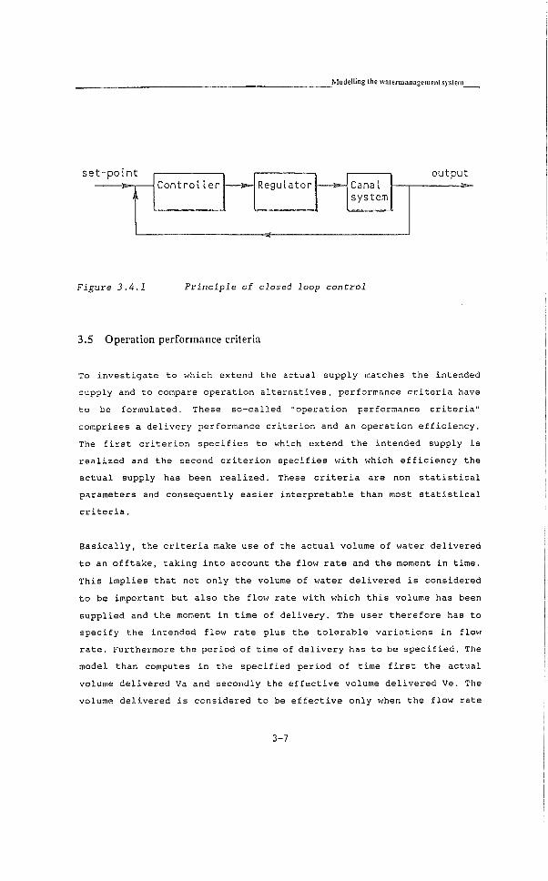
s i g n a l ( F i g . 3.4.1). I n t h i s way the pumping s t a t i o n can be switched
on/off depending on the a c t u a l upstream water l e v e l . The c o n t r o l l e r reads
the a c t u a l water l e v e l and then determines whether the pumping s t a t i o n
should be switc h e d on or o f f .
The output s i g n a l i s p r e - d e f i n e d f u n c t i o n of an other v a r i a b l e . I n the
example of the pump, the d i s c h a r g e i s a pre-d e s c r i b e d f u n c t i o n of the
upstream water l e v e l , i n which the water l e v e l i s c a l l e d the f u n c t i o n
v a r i a b l e . The f o l l o w i n g f u n c t i o n v a r i a b l e s are standard a v a i l a b l e i n
MODIS:
- upstream water l e v e l
upstream water l e v e l head (- water l e v e l - s i l l l e v e l )
Ratio of the upstream and downstream head
Advanced closed loop controllers
The c o n t r o l l e r s mentioned above, are probably the s i m p l e s t type of c l o s e d
loop c o n t r o l l e r s . I n MODIS more s o p h i s t i c a t e d c l o s e d loop c o n t r o l l e r s
have been implemented as w e l l . With these s o p h i s t i c a t e d c o n t r o l l e r s the
output v a l u e i s computed by the c o n t r o l l e r and not by a p r e - d e s c r i b e d
f u n c t i o n . I n MODIS the f o l l o w i n g type of advanced c l o s e d loop c o n t r o l l e r s
have been implemented:
- s t e p c o n t r o l l e r with dead band
P I D - c o n t r o l l e r with speed l i m i t a t i o n
With t h e s e advanced c o n t r o l l e r s i t i s p o s s i b l e for example, to si m u l a t e
the behaviour of a system equipped with automatic upstream and downstream
c o n t r o l l e d water l e v e l r e g u l a t o r s .
3-6
Modelling the watermanagetnentsjsteni
s e t - p o i n t C o n t r o l l e r R e g u l a t o r C a n a I
s y s t e m
o u t p u t
Figure 3.i.l Principle of closed loop control
3.5 Operation performance criteria
To i n v e s t i g a t e t o which extend the actual supply matches the intended
supply and to compare operation a l t e r n a t i v e s , performance c r i t e r i a have
to be formulated. These so-called "operation performance c r i t e r i a "
comprises a d e l i v e r y performance c r i t e r i o n and an operation e f f i c i e n c y .
The f i r s t c r i t e r i o n s p e c i f i e s t o which extend the intended supply i s
r e a l i z e d and the second c r i t e r i o n specifies w i t h which e f f i c i e n c y the
actual supply has been r e a l i z e d . These c r i t e r i a are non s t a t i s t i c a l
parameters and consequently easier i n t e r p r e t a b l e than most s t a t i s t i c a l
c r i t e r i a .
B a s i c a l l y , the c r i t e r i a make use of the actual volume of water delivered
t o an o f f t a k e , t a k i n g i n t o account the flow r a t e and the moment i n time.
This implies t h a t not only the volume of water d e l i v e r e d i s considered
t o be important but also the flow rate w i t h which t h i s volume has been
supplied and the moment i n time of d e l i v e r y . The user th e r e f o r e has to
specify the intended flow rate plus the t o l e r a b l e v a r i a t i o n s i n flow
r a t e . Furthermore the period of time of d e l i v e r y has t o be s p e c i f i e d . The
model than computes i n the specified period of time f i r s t the actual
volume delivered Va and secondly the e f f e c t i v e volume de l i v e r e d Ve. The
volume delivered i s considered t o be e f f e c t i v e only when the flow rate
3-7
User's guide MODIS
is i n between the t o l e r a b l e range of flow rates.
Delivery performance
When the e f f e c t i v e volume Ve i s at l e a s t equal t o the intended volume V i ,
the d e l i v e r y performance i s p e r f e c t . For the o f f t a k e receives no d e f i c i t
of water. This pe r f e c t performance r e s u l t s i n a d e l i v e r y performance
r a t i o (DPR - Ve/Vi) of 100%.
Operation efficiency
However, there might s t i l l be losses of water. The losses consist of
water which i s supplied not w i t h i n the s p e c i f i e d range of flow rates
and/or the volume supplied above the intended volume. The amount of
losses are r e f l e c t e d i n the operation e f f i c i e n c y eo (e^ - Ve/Va). An
operation e f f i c i e n c y of 100% i n d i c a t e s t h a t no water i s l o s t . However,
i t does not stat e anything about the d e l i v e r y performance. The operation
e f f i c i e n c y i s part of the conveyance e f f i c i e n c y as defined by the ICID
(Bos 1978).
3.6 Accuracy and stability
3.6.1 Numerical accuracy
The user of MODIS, and of any hydrodynamic flow model i n general, should
be w e l l aware of the f a c t t h a t the model can only provide an
approximation of the exact s o l u t i o n of the de Saint Venant equations.
This i s an i n e v i t a b l e consequence of using d i s c r e t i z e d equations. (For
a more d e t a i l e d discussion of the mathematical backgrounds of MODIS,
reference i s made t o chapter 11 and 1 2 ) . Furthermore, the model r e s u l t s
can only be as accurate as the (measured) input data describing the
watermanagement system.
Accuracy of model computations
MODIS makes use of some computational parameters (Ax, At and 6), w i t h
which the user can influence the accuracy of the model computations. One
3-8
Modelling lhe w a t e r m a n a g e m e n l 5 ) S t e m _
must r e a l i z e t h a t the mesh size Ax and the time step At used t o
d i s c r e t i z e the time space f i e l d , cannot be chosen at random. They must
stand i n reasonable r e l a t i o n t o the dimensions (wave length) and time
scale under i n v e s t i g a t i o n , as w e l l as i n a c e r t a i n p r o p o r t i o n to each
other. Furthermore, the value of the time i n t e r p o l a t i o n c o e f f i c i e n t $
should be c a r e f u l l y selected. I n general i t can be stated t h a t the
simulation i s most accurate when Ax and At are as small as possible, the
Courant number i s equal t o u n i t y and the time i n t e r p o l a t i o n c o e f f i c i e n t
0 i s equal t o 0.5.
Mesh size Ax
The selected mesh size Ax i s r e l a t e d t o the problem under i n v e s t i g a t i o n .
For an accurate representation of a backwater curve f o r example, several
g r i d points should be located i n t h a t backwater curve. This usually
r e s u l t s i n a mesh size of order 100 m. For the representation of waves,
the distance between two g r i d p o i n t s should not exceed the wave length.
Usually the wave length increases i n time, due t o d i f f u s i o n . The small
wave lengths u s u a l l y increase i n short time (order minutes) t o an order
of 100 m, r e s u l t i n g i n a mesh size of order of 100 m. In many simulations
one i s not i n t e r e s t e d i n an accurate simulation of the small waves, as
the water volume involved i s small as w e l l . However, i n case of closed
loop c o n t r o l systems, an accurate representation of the small waves i s
often e s s e n t i a l f o r a proper s i m u l a t i o n of the c o n t r o l l e d system.
Time step At
The chosen time step At should be r e l a t e d t o the mesh size Ax. The
numerical s o l u t i o n r e l a t e d to the wave c e l e r i t y i s most accurate when the
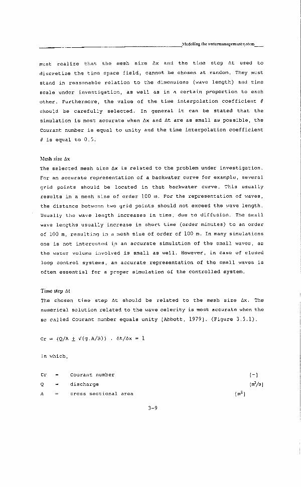
so c a l l e d Courant number equals u n i t y [Abbott, 1979]. (Figure 3.5.1).
Cr - {Q/A + N^(g.A/B)> At/Ax - 1
In which
Cr Courant number l - l
Q d i s c h a r g e (mVs)
A cross s e c t i o n a l area
3-9
User's guide M0D1S_
B - canal surface w i d t h [m]
g - a c c e l e r a t i o n of g r a v i t y IW^]
The Courant number i s not the only parameter t h a t determines the time
step. I t should be noted t h a t the accuracy of the r e g u l a t o r s and
c o n t r o l l e r s i s also e f f e c t e d by the time step. The equation of the flow
through the r e g u l a t o r i s l i n e a r i z e d and consequently only v a l i d i n a
small range around the a c t u a l s t a t e . For an accurate computation of
considerable v a r i a t i o n s , s u f f i c i e n t intermediate computations have t o be
made, r e s u l t i n g i n small time steps. The same story holds t r u e f o r the
c o n t r o l l e r .
2
Figure 3.5,1 Accuracy of model computation related to wave
propagation celerity as a function of the number of
grid points per wave length and the Courant number
(Cr) . The time Interpolation coefficient (S) Is 0.5.
Courant numbers greater than unity cause the computed
wave to travel faster than In reality (Rubicon 198i).
3-10
.Modelling the watermanagement systeni_
Time interpolation coefficient 0
The value of the time i n t e r p o l a t i o n c o e f f i c i e n t 6 a f f e c t s the wave
deformation and should always be w i t h i n the range 0.5 -1.0. A value f o r
8 l a r g e r than 0.5 leads t o damping of the wave, sometimes r e f e r r e d t o as
a r t i f i c i a l or numerical d i f f u s i o n . However, some a r t i f i c i a l d i f f u s i o n i s
desir a b l e i n order t o damp small f l u c t u a t i o n s which r e s u l t from round of
er r o r s . Therefore u s u a l l y a value of 0 i s selected of about 0.55 t o 0.60.
A value of 1.0 can be used when a r t i f i c i a l numerical d i f f u s i o n i s
desi r a b l e , f o r instance during a steady sta t e run.
Concluding remarl<s
Accurate computations w i l l lead to more computation time. Therefore
always a compromise should be found between accuracy and computation
speed. The user of MODIS should be w e l l aware t h a t the r u l e s f o r accuracy
of conventional flow models are not s u f f i c i e n t f o r MODIS i n which closed
loop c o n t r o l l e d systems can be simulated. The proper time step i s
determined by the flow i n the canals, the regul a t o r and the c o n t r o l l e r .
A p r a c t i c a l and simple measure t o evaluate the accuracy of the
computations, i s t o repeat the computation w i t h other (smaller) parameter
values and compare the r e s u l t s . On a c e r t a i n moment the r e s u l t s w i l l not
s i g n i f i c a n t l y change which indicates t h a t i t i s of no use t o f u r t h e r
reduce the parameter values.
3.6.2 Numerical stability
Concerning the question of s t a b i l i t y i t should be noted t h a t an i m p l i c i t
numerical scheme i s used, which guarantees a numerical stable s o l u t i o n ,
when the time i n t e r p o l a t i o n c o e f f i c i e n t $ i s l a r g e r than 0.5. ( S t a b i l i t y
has been defined i n t h i s user's guide as damped f l u c t u a t i o n s ) . Although
a s t a b l e numerical scheme i s used, undesired f l u c t u a t i o n s might occur.
To damp these f l u c t u a t i o n s , the time i n t e r p o l a t i o n c o e f f i c i e n t 8 should
be taken some closer t o u n i t y . However, i t i s w e l l possible, e s p e c i a l l y
due t o the use of closed loop c o n t r o l , t h a t physical i n s t a b i l i t y occurs.
In t h a t case, the user should not t r y t o damp these f l u c t u a t i o n s but be
aware of the physical o r i g i n .
3-11
User's guide MODIS ^ _
Furthermore non-linear i n s t a b i l i t y might occur. Non-linear i n s t a b i l i t y
r e s u l t s from l i n e a r i z i n g the resistance c o e f f i c i e n t and canal parameters
such as the surface width and the cross-sectional area. I n MODIS sp e c i a l
care has been taken t o avoid these non-linear s t a b i l i t y problems, by
i t e r a t i n g the computation (at least twice) and by evaluating the
parameter values i n between two time l e v e l s (see chapter 7 ) .
The non-linear i n s t a b i l i t y i s i n f a c t a r e s u l t of an inaccurate
computation and can be avoided by reducing the computational time step
At. I n p r a c t i c e i n s t a b i l i t y mostly occur during a steady s t a t e run.
Possible remedies i n t h a t case are:
- reducing the time step At
a more accurate d e f i n i t i o n of the i n i t i a l s t a t e .
a time i n t e r p o l a t i o n c o e f f i c i e n t 8 equal t o 1.0
A f i n a l s o l u t i o n i s to s i m p l i f y the canal c o n f i g u r a t i o n by c l o s i n g
some o f f t a k e s structures and opening them gradually during the run.
The even t u a l l y obtained steady state can be used as an i n i t i a l s t a t e f o r
f u r t h e r simulations.
3 .7 Model calibration
3.7.1 Accuracy of input data
The accuracy of the model r e s u l t s i s only as good as the input data.
(This does not imply t h a t inaccurate model simulations can be used when
the accuracy of the input data i s poor. I t i s j u s t the opposite. When the
input data i s poor, accurate simulations should be made as not t o
increase u n c e r t a i n t y ) . The required accuracy of the input data i s r e l a t e d
t o the desired accuracy of the model r e s u l t s .
Canal system
Normally the canal lay-out and canal length i s known from maps. By
3-12

Modelling the watermanagementsystera
modelling the c o n f i g u r a t i o n , too d e t a i l e d modelling should be avoided.
Small i n f l o w or o f f t a k e s can o f t e n be combined i n t o one greater i n f l o w
or o f f t a k e p o i n t .
The canal p r o f i l e s may a l t e r i n time and are f r e q i j e n t l y d i f f e r e n t from
the designed p r o f i l e s . The shape of the canal p r o f i l e and the bottom
l e v e l s are not so important because the model r e s u l t s are not very
s e n s i t i v e t o those data. Consequently very d e t a i l e d modelling of cross-
sections i s not required. Besides, possible e r r o r s can be compensated
wit h the resistance c o e f f i c i e n t . The flow width of the canal section
should be measured more accurately because t h i s determines the storage
area of the canal and consequently e f f e c t s the response time of the canal
system considerably.
The resistance of the canal cannot be measured e x p l i c i t l y and should be
determined i n the c a l i b r a t i o n stage.
Regulators
The dimensions of the regulators are important as the flow i s very
s e n s i t i v e f o r v a r i a t i o n s i n dimensions. In p r a c t i c e , the actual s t a t e of
many regulators i s q u i t e d i f f e r e n t from the o r i g i n a l state and therefore
i t i s worthwhile t o check a l l regulators before modelling.
Boundary conditions
F i n a l l y the boundary conditions must be measured accurately. P a r t i c u l a r l y
the accuracy of the i n f l o w and the seepage (outflow) determine t o a great
extend the accuracy of the model r e s u l t s . Other boundary conditions can
be taken so f a r downstream t h a t they do not e f f e c t the model r e s u l t s .
3.7.2 Calibration
C a l i b r a t i o n i s a process of determining the best value of some
( c a l i b r a t i o n ) parameters by comparing r e a l l i f e measurement data w i t h
model simulation r e s u l t s . Model c a l i b r a t i o n i s necessary only when an
already e x i s t i n g water management system i s modelled. In the design phase
of new systems, no c a l i b r a t i o n i s needed and consequently i t i s not
3-13

User's guide MODIS
always needed t o use c a l i b r a t i o n data f o r MODIS. The main variable to be
determined i n the c a l i b r a t i o n phase i s the resistance c o e f f i c i e n t . This
value may vary i n time and space. Furthermore checks have t o be made t o
confirm the magnitude of storage widths.
Verification
For c a l i b r a t i o n several r e a l l i f e measurement data sets are required,
some of them are used t o determine the value of the c a l i b r a t i o n
c o e f f i c i e n t s and others are used t o v e r i f y the c a l i b r a t e d parameters i n
order t o r a i s e the l e v e l of confidence i n the simulation r e s u l t s .
Steady state
Normally c a l i b r a t i o n i s f i r s t c a r r i e d out i n a steady state condition.
This c o n d i t i o n i s achieved by keeping constant the inflow and gate
openings. I n order t o compute the resistance parameter, i t i s advised t o
close as many gates as possible as not t o d i s t u r b the computations by
c a l i b r a t i o n e r r o r s of the regu l a t o r s and non-uniform flow conditions
(backwater curves). The same data sets can be used t o estimate the amount
of seepage losses (when the s t r u c t u r e s have been closed or c a l i b r a t e d
a c c u r a t e l y ) .
Simultaneously the regulators can be c a l i b r a t e d . However, i t i s most
important t o measure the r i g h t dimensions of the structures. The
discharge c o e f f i c i e n t s can o f t e n be obtained from l i t e r a t u r e or a
t h e o r e t i c a l analyses. The e r r o r made i s o f t e n small.
Unsteady state
I n a d d i t i o n t o the steady st a t e c a l i b r a t i o n an unsteady state c a l i b r a t i o n
can be c a r r i e d out i n order t o check the measured input data and the
previou s l y computed resistance c o e f f i c i e n t . I n an unsteady c a l i b r a t i o n
the discharge at the intake i s increased and at several locations the
flow r a t e and water l e v e l i s measured at c e r t a i n i n t e r v a l s of time. The
propagation c e l e r i t y of the disturbance i s mainly determined by the
storage width and the resistance i n the canal. The measured data set can
be used t o v e r i f y these model parameters.
3-14

Modelling the w atermanagement system̂
I n a d d i t i o n the measured r e s u l t s can be used t o r a i s e the l e v e l of
confidence i n the model s i m u l a t i o n r e s u l t s by comparing measured and
s i m u l a t e d response time. However, c a l i b r a t i o n should i n g e n e r a l not be
used t o v e r i f y the concept- of the model. C a l i b r a t i o n i s p r i m a r i l y
r e q u i r e d t o a s s e s c e r t a i n parameter v a l u e s such as the r e s i s t a n c e
c o e f f i c i e n t .
3-15

User's guide MODIS

4 Input data files
4.1 Structure of input data files
Input data i s read by MODIS from input f i l e s . The input f i l e s which have
to be defined by the user are s i m i l a r t o t e x t f i l e s used i n word
processing. Each executable sub-program of the program package needs one
user defined input f i l e . R l l the user defined input f i l e s have a standard
s t r u c t u r e . An input f i l e i s b u i l t up of input segments, which i n t u r n are
b u i l t up of input blocks.
Input segments
Each input f i l e i s d i v i d e d i n t o input segments. An input segment i s a
group of input data of the same nature. For example, there i s an input
segment f o r the d e f i n i t i o n of branches and nodes, and another input
segment has been reserved f o r the d e f i n i t i o n of s t r u c t u r e s . No special
character has t o be given t o mark the beginning of an input segment.
However, each input segment i s closed by an input l i n e containing the
symbols "*END" i n the f i r s t four columns of the data f i l e .
Input blocks
Each input segment i n t u r n consist of one or more input blocks. For
example the input segment "structures" consist of a block f o r overflow
s t r u c t u r e s , a block f o r underflow s t r u c t u r e s , et cetera. The beginning
of an input block i s marked by a so-called steer-key. (A steer-key i s a
word s t a r t i n g w i t h the steer symbol "*" i n the f i r s t column). For the
input block overflow s t r u c t u r e s e.g., the steer key reads "*WEIR". The
input block i s closed by l i n e containing the character "-" i n the f i r s t
column.
4 - 1

4.2 Data conventions
The input data of the user defined input f i l e i s format-free which
implies t h a t the l o c a t i o n of the data along an input l i n e i s not
important, and only the sequence should f o l l o w the g u i d e l i n e s . However,
even format-free data processing has t o f o l l o w some conventions. The
general data conventions are:
- data items have t o be given at a l l places where an in p u t i s
expected;
a l l input items are separated by at le a s t one blank character;
- No data should be given i n the f i r s t column. The characters
given i n the f i r s t column has a spec i a l meaning.
The symbols used i n the f i r s t column are " + ", "-", and " = " . The
meaning of these symbols has been l i s t e d beneath:
+ comment l i n e . Data s p e c i f i e d on t h i s l i n e i s not read by the program
but copied t o the echo f i l e . The echo f i l e i s an echo of the input
f i l e i n which error messages are include.
- comment l i n e . Data s p e c i f i e d on t h i s l i n e i s also not read by the
program but i t i s not copied t o the echo f i l e .
* steer key, used t o mark the beginning of an input block or the end
of an input segment (*END).
= used t o mark the end of an input block;
I f the f i r s t column i s l e f t blank, t h i s i n d i c a t e s a normal data l i n e .
Data given on t h i s l i n e are read by the model
Note
Where i n t h i s d e s c r i p t i o n i t has been s p e c i f i e d t h a t data are given on
one l i n e , a l l data should indeed be given on t h a t l i n e and not continued
on another l i n e . The f i e l d length of the l i n e s i s i n p r i n c i p l e l i m i t e d
t o 80 characters. (However f o r some i n s t a l l a t i o n s another f i e l d length
i s p e r m i t t e d ) . Comment l i n e s can be included anywhere i n the i n p u t . The
use of "+" characters i n the f i r s t column i s e s p e c i a l l y useful as heading
4-2

Input data IBes
f o r input data, whereas, the "-" characters can be used f o r deactivating
data l i n e s temporarily. An example of an input data f i l e i s given i n Fig
4.2.1.
»ORIF
BRANCH DIR
FSl
FS2
fS3
FS4
FS7
FS8
FS9
FSIO
BPl
BPl
BP2
BP2
2998.0 PX
9998.0
14002.0
21998.0
29298.0
29598.0 -
29998.0
38002.0
1.0 0.63 10 28.65
27.55
27.55
26.75
23.10
21.85
20.55
18.40
0.30
0.55
LA$CNTR3
0.90
0.53
0.53
0.55
LASCNTRIO
*UEIR
+ NAME
WS3
US9
BS3
BS9
5.0
5.0
PX
PX
OTSFRED 1.0 1.5 12.0 TTSOFFl
1.5 12.0 TT$0FF2
'END o f ADODEF
•AULC AUTOMATIC LOCAL CONTROL
+ NAME CONTROL TYPE I n i v a t TARGET Kp Ki Kd SPEED HIN MAX
CNTR3 PID uc 0.23 30.15 -3.0 -1.8 0.5 0.5 O.O 2.0
CNTRIO PIO uc 0.34 20.17 -3.0 -1.8 0.5 1.5 0.0 2.0
•END o f a u t o m a t i c c o n t r o l l e r s
•TTIH TABULATED FUNCTIONS OF TIME
QINFLOW OFFl 0FF2
00:00:00:00 10.0 29.872 19.892
00:07:59:00 - . •
00:08:00:00 13.0 29.872 19.97
05:00:00:00 - . .
Figure It.2.1 Example of a part of an input data file
4-3

User's guide MODIS_
4.3 Data types
Data items can be of three d i f f e r e n t types:
r e a l value f i g u r e s , characterized by a f i g u r e which may contain
a p o i n t but not necessarily (e.g. 10.35 but also 10);
i n t e g e r value, characterized by a f i g u r e containing no p o i n t
(e.g. 10, 1232);
a character s t r i n g , characterized by a mixture of a l p h a b e t i c a l
and numerical characters (e.g. STRUCTl, BRAMCH2).
Character s t r i n g s do not have t o be enclosed i n quotes ('). I f these are
s p e c i f i e d , they form part of the character s t r i n g . I t i s advised t o work
always w i t h c a p i t a l characters because the model d i s t i n g u i s h e s normal and
c a p i t a l characters which might lead t o misunderstandings.
Names consist of any ANSI defined symbols and usually f o l l o w the
convention t h a t the length does not exceed 10 characters. Any characters
f o l l o w i n g these 10 characters are truncated. The names should never
contain blanks as t h i s symbol has been reserved f o r separating input
items. Instead of a blank the characters "-" may be used t o form
composite names. (So "BRANCH 2" i s wrong but "BRANCH_2" i s c o r r e c t )
A l l input data have t o be given i n S l - u n i t s , except f o r the time which
i s given i n a DHMS-notation (Days-Hours-Minutes-Seconds) as
DDD:HH:MM:SS. (e.g. 5:10:28:15 stands f o r 6 days, 10 hours, 28 minutes
and 15 seconds).
4.4 Special information characters
To f a c i l i t a t e easy input s p e c i f i c a t i o n , the user can replace input data
by so-called SIF-characters, s p e c i a l Information Characters. A s e l e c t i o n
can be made out of the f o l l o w i n g SIF-characters:
4-4

Input iLatn filta
# s u b s t i t u t e the d e f a u l t value or name s p e c i f i e d i n the program f o r
t h i s v a r i a b l e (can be used only i n a l i m i t e d number of places);
value or name i s set equal t o what has been given i n the same data
column on the previous l i n e ;
< value or name i s set equal t o what has been given i n the l e f t hand
neighbouring data column on the same l i n e ;
> value or name i s set equal t o what has been given i n the r i g h t hand
neighbouring data column on the same l i n e ;
? i n t e r p o l a t i o n of values or functions between data given above and
below i n the same data column.
In Fig. 4.2.1, these special information characters have been used too.
4-5

L'ser's guide MODIS
5 Model definition
5.1 Introduction
I n the subsystem Model D e f i n i t i o n (MODDEF) Che c o n f i g u r a t i o n and che
h y d r a u l i c c h a r a c t e r i s t i c s of Che open water sysCem are defined. The input
f i l e of the model d e f i n i t i o n i s u s u a l l y c a l l e d DEFIN.DAT. I f a new input
f i l e i s made i t i s a d v i s e d to modify an e x i s t i n g input f i l e i n s t e a d of
making a complete new input f i l e . A l l standard data such as run c o n t r o l
parameters, do not have Co be Cyped a g a i n and only Che daCa d e s c r i b i n g
Che i r r i g a t i o n sysCera can be a l C e r e d .
The input f i l e of Che model d e f i n i t i o n ( u s u a l l y c a l l e d DEFIN.DAT)
c o n s i s t s of seven inpuC segraenCs. As a s p e c i a l f a c i l i c y f o r slow computer
sysCeras each segraenC can be pro c e s s e d i n d i v i d u a l l y . However, Co avoid
i n c o n s i s t e n c y i C i s a d v i s e d Co r e p r o c e s s Che complete inpuC f i l e i f
changes are made.
I n Table 5.1.1 a l l inpuC segmenCs and the sCeer-keys of C h e i r inpuC
b l o c k s a re presenced. I n che f o l l o w i n g of t h i s chapCer each input segmenC
i s d i s c u s s e d i n d e C a i l .
5-1

L W s guide MODIS_
T A B L E S.1.1 Description of the input segments of model defmition
Segment; D e s c r i p t i i o n Input B l o c k s F u n c t i o n
number
1 i d e n t i f i c a t i o n *IDEN run i d e n t i f i c a t i o n
*SWIT run s w i t c h e s
2 net d e f i n i t i o n *NODE d e f i n i t i o n of nodes
*BRAN d e f i n i t i o n of branches
3 g r i d d e f i n i t i o n *CROS c r o s s - s e c t i o n a l data
*TRAP t r a p e z o i d a l c r o s s - s e c t i o n s
*GRID d e f i n i t i o n of g r i d p o i n t s
A s t r u c t u r e s *LATQP l a t e r a l p o i n t flows
*WEIR overflow s t r u c t u r e s
*ORIF underflow s t r u c t u r e s
*PIPE pipe opening s t r u c t u r e s
*LOST head l o s s s t r u c t u r e s
*PUMP pumps
*NERP n e y r t e c d i s t r i b u t o r s
*FDST f o r t r a n d e f i n e d s t r u c t u r e s
5 automatic c o n t r o l *AULC automatic l o c a l c o n t r o l l e r s
*AURC automatic remote c o n t r o l l e r s
6 f u n c t i o n s *TGFU t a b u l a t e d g e n e r a l f u n c t i o n s
*TTIM t a b u l a t e d time f u n c t i o n s
*FDFU f o r e r a n d e f i n e d f u n c t i o n s
7 i n i t i a l data *INST i n i t i a l data of the system
5-2
Modd defiiutiou
5.2 IdentiFicatioii
The i n p u t segment IDENTIFICATION c o n s i s t of two input b l o c k s ( s e e a l s o
Table 5.1.1);
*IDEN f o r g i v i n g the run i d e n t i f i c a t i o n parameters and
*SWIT f o r s e t t i n g the run s w i t c h e s .
Normally the u s e r can leave t h i s input segmenC unchanged. Only i f the
name of the i n and output f i l e s a re changed input block *IDEN should be
used.
S .2 .1 Run Identification
The i d e n t i f i c a t i o n block s t a r t s a f t e r the s t e e r - k e y *IDEN w i t h 3 l i n e s
c o n t a i n i n g a standard code which i s followed, a f t e r a t l e a s t one blank,
by a u s e r - d e f i n e d code or t e x t . T h i s code or t e x t should not s t a r t
before column 20.
This first part has the form:
RUN DESCRIPTION us e r s s p e c i f i e d t e x t (max 40 c h a r a c t e r s )
RUN CODE u s e r s s p e c i f i e d code (5 c h a r a c t e r s )
EXECUTED BY u s e r s s p e c i f i e d name (max 40 c h a r a c t e r s )
The codes i n c a p i t a l s have to be copied e x a c t l y .
The second p a r t c o n s i s t s of information concerning f i l e names. The model
MODDEF must know the name of the input f i l e and the names of the output
f i l e s produced by MODDEF.
The i n p u t - , echo- and output f i l e s have to be s p e c i f i e d i n the job
c o n t r o l f o r executing the job. The model data base and the r e s u l t data
base f i l e names are needed to w r i t e the r e s u l t s i n unformatted form Co
the r i g h t f i l e s . The names s p e c i f i e d by the u s e r here a l s o should not be
given b e f o r e column 20.
5-3
L W s gukfe MODIS_
T h i s second p a r t has now the form:
INPUT f i l e name
ECHO f i l e name
OUTPUT f i l e name
MODELDB f i l e name
RESULDB f i l e name
c o n s i s t e n t w i t h Job c o n t r o l
defined here
The codes i n c a p i t a l s have to be copied a g a i n e x a c t l y . At the end of t h i s
input b l o c k a l i n e i s given w i t h the c h a r a c t e r '-' i n the f i r s t column.
An example of the input block *IDEN i s given i n F i g . 5.2.1
*IDEN
+
RUN IDENTIFICATION
< >
RUN-DESCRIPTION (AO CHARS: MODIS RUN 1
< >
RUNCODE : T E S T l
< >
EXECUTED BY : TU DELFT
DATASET (FILENAMES)
< >
INPUT DEFIN.DAT (JCL.MODIFY)
ECHO DEFECH.DAT
OUTPUT DEFOUT.DAT "
MODELDB USMDB.UNF
SST-FILE USSST.UNF
Fig. 5.2.1 Example of input block *IDEN (run identification)
5-4

Modé defiiiitioa
5.2.2 Switches
The run s w i t c h e s block begins w i t h the s t e e r - k e y *SWIT, followed by three
data l i n e s each c o n t a i n i n g 7 sw i t c h e s . The sw i t c h parameters a c t i v a t e or
d e a c t i v a t e data t r a n s f e r , b l o c k s of swi t c h e s , debug f a c i l i t i e s ,
p r o c e s s i n g of input segments and the p r i n t i n g of t h e i r r e s u l t i n g output.
These s w i t c h e s have to be given i n a s p e c i f i c sequence. To i n d i c a t e the
names, th e s e appear i n a l i s t on a comment l i n e . On the next i n p u t l i n e
the f o l l o w i n g c h a r a c t e r s can be given;
Y - a c t i v a t e s the s w i t c h ( a b b r e v i a t i o n of YES);
N - d e a c t i v a t e s the s w i t c h ( a b b r e v i a t i o n of NO ) ;
On each l i n e 7 switches are read. Some p o s i t i o n s have no meaning y e t as
i n d i c a t e d by the heading 'FREE'. Here the d e f a u l t c h a r a c t e r has to
be g i v e n .
The s w i t c h e s w i t h t h e i r meaning are given below i n the sequence i n which
they appear i n the input.
l i n e 1
NEWMODDB
WRMODDB
DEFALL
OUTALL
DEBUGOUT
FREE
FREE
c r e a t e s a new model data base
w r i t e s processed r e s u l t s to the model data base
s e t s a l l the switches of l i n e 2 to YES
s e t s a l l the switches of l i n e 3 to YES
swit c h e s debugging output on
res e r v e d f o r extensions
l i n e 2
DEFNET - s w i t c h f o r p r o c e s s i n g net d e f i n i t i o n i n input
DEFGRD - . . . . N gj-id
DEFFUN " f u n c t i o n
DEFINI - . . . . " i n i t i a l data "
5-5
User's guide MODIS_
DEFIAT - 11 II " l a t e r a l flow " "
DEFSTRUC - " s t r u c t u r e
DEFACS . " " automatic c o n t r o l systems "
l i n e 3
S i m i l a r as l i n e 2 f o r producing outputs of the segments.
An example of the input segment *SWIT i s given i n F i g . 5.2.2
*SWIT- RUN SWITCHES
+
+ NEWMODDB WRMODDB
Y Y
+ DEFNET DEFGRD
Y Y
+ OUTNET OUTGRD
Y Y
Y-YES N-NO
DEFALL OUTFALL
N N N
DEFFUN DEFINI DEFLAT
Y Y Y
OUTFUN OUTINI OUTFLAT
Y Y Y
DEBEGOUT FREE
// //
DEFSTRU DEFACS
Y Y
OUTSTRUC OUTACS
Y Y
Fig. 5.2.2 Example of input block * SWIT (run switches).
Tip
I f a steady s t a t e has been made and t h i s steady s t a t e i s used as the
i n i t i a l s t a t e ( c h a p t e r 6 ) , the model should not process the i n i t i a l s t a t e
of the Model D e f i n i t i o n any more. To d e - a c t i v a t e the p r o c e s s i n g o f the
i n i t i a l s t a t e , the s w i t c h e s f o r DEFINI and OUTINI, should be s e t on N.
However, i f the c a n a l c o n f i g u r a t i o n i s changed, the s w i t c h e s should f i r s t
be s e t on Y, t i l l a new steady s t a t e has been made (see chapter 6 ) .
5-6

Nïodel dfefinitioQ
5.3 Net definition
The input segment Net D e f i n i t i o n c o n s i s t of two input b l o c k s :
*NODE f o r the d e f i n i t i o n of nodes, and
*BRAN f o r the d e f i n i t i o n of branches.
5.3.1 Nodes
The I d e n t i f i c a t i o n l i n e f o r the node d e f i n i t i o n input block i s :
* NODE - DEFINITION OF NODES
+
+ NAME TYPE CONNECTING BOUNDARY
+ BRANCH(ES) VALUE/REFERENCE
The data given i n the l i n e s s t a r t i n g w i t h the c h a r a c t e r "+" i n the f i r s t
column are ( o p t i o n a l ) comment l i n e s .
Data f o r each node are given on a new l i n e . I n t e r n a l l y the node names are
transformed i n t o numbers. The numbering f o l l o w s from the sequence i n
which nodes are s p e c i f i e d i n the inp u t . ( T h i s i m p l i e s t h a t the sequence
a l s o i n f l u e n c e s the band width of the c o e f f i c i e n t m a t r i x of the r e s u l t i n g
node equations and hence the computer time r e q u i r e d f o r s o l v i n g t h i s
system of e q u a t i o n s ) .
For each node the fo l l o w i n g data i s r e q u i r e d :
NAME : name of the node. Any name composed of ANSI
c h a r a c t e r s i s allowed. The len g t h i s l i m i t e d to
10 c h a r a c t e r s .
TYPE : type of node c o n d i t i o n (boundary c o n d i t i o n ) ; The
type i s gi v e n as a c h a r a c t e r s t r i n g composed, i n
most c a s e s , of two p a r t s : an i d e n t i f i c a t i o n f o r
the boundary type (node type) and the way i n
which data a re given (data t y p e ) . See Table 5.3.1
for p o s s i b l e node types.
5-7

L W s guide MODIS_
I n p r i n c i p l e any number of branches can be
connected a t a node. I n the a c t u a l input
p r o c e s s i n g , however, the number i s l i m i t e d to 7
(supposing t h a t the a r r a y l i m i t KNMAX has been
s e t to 7 i n the c o m p i l a t i o n ) . The names of these
branches can be given i n random order. A u s e f u l
convention i s to go around the node i n c l o c k w i s e
d i r e c t i o n . The l e n g t h of the branch names again,
a r e l i m i t e d to 10 c h a r a c t e r s .
Where the data type has been s p e c i f i e d as
c o n s t a n t , the v a l u e can be s u b s t i t u t e d here
d i r e c t l y e i t h e r as an i n t e g e r or as a r e a l v a l u e .
Where data are given i n the form of a t a b u l a t e d
or F o r t r a n f u n c t i o n , r e f e r e n c e i s made here to
the f u n c t i o n name. The data should be g i v e n i n
the input p a r t f o r the f u n c t i o n s .
I f a l l nodes have been s p e c i f i e d the input l i s t f o r nodes i s c l o s e d w i t h
a l i n e c o n t a i n i n g the "-" c h a r a c t e r i n the f i r s t column.
TABLE 5.3.1 Type of node conditions
H water l e v e l given;
Q d i s c h a r g e given;
QH d i s c h a r g e - stage r e l a t i o n s h i p ;
CF c r i t i c a l outflow c o n d i t i o n ;
JW j u n c t i o n w i t h water l e v e l c o m p a t i b i l i t y c o n d i t i o n (no
s t o r a g e ) ;
JS j u n c t i o n as JW with storage (e.g. f l o o d p l a i n c e l l ) .
The v a l u e of each type of node c o n d i t i o n can be given as;
C c o n s t a n t v a l u e ;
T t a b u l a t e d f u n c t i o n ;
F F o r t r a n - d e f i n e d f u n c t i o n ;
CONNECTING BRANCHES
BOirNDARY V A L U E
5-8

Modd m.
g i v e n
i n the
the
w a t e r
From these options the f o l l o w i n g combinations are p o s s i b l e :
HC - water l e v e l g iven as a constant v a l u e . The v a l u e i _
w i t h r e f e r e n c e to the ge n e r a l model datum l e v e l ;
HT - water l e v e l g iven as a t a b u l a t e d f u n c t i o n of time ;
HF - water l e v e l g iven by any u s e r - d e f i n e d d e s c r i p t i o n
form of a F o r t r a n f u n c t i o n ;
QC - d i s c h a r g e given as a constant v a l u e (e.g. Q - 0 ) ;
QT - d i s c h a r g e given as a t a b u l a t e d f u n c t i o n of time;
QF - d i s c h a r g e given by any u s e r - d e f i n e d d e s c r i p t i o n
form of a F o r t r a n f u n c t i o n ;
QHT - d i s c h a r g e given as a t a b u l a t e d f u n c t i o n of t h e
l e v e l ;
QHF - d i s c h a r g e given as a f u n c t i o n of the water l e v e l s p ^ . ^ I f i e d
by the u s e r i n the form of a F o r t r a n f u n c t i o n .
CF - c r i t i c a l outflow from the channel at the node. T h e p a r a
meters f o l l o w from the channel c r o s s - s e c t i o n aC t h e node;
JW - water l e v e l c o m p a t i b i l i t y a t the node. Where energ;y. ^
c o m p a t i b i l i t y i s p r e f e r r e d the boussinesq c o e f f i c j ^ ^ ^
can be s e t equal to zero.
JSC - storage node w i t h water l e v e l c o m p a t i b i l i t y and s t-^ o r a g e
d e f i n e d as a constant value; JST - storage node w i t h storage given as a t a b u l a t e d f u n c t i
•^on of the water l e v e l ;
J S F - storage node w i t h storage d e f i n e d through a Po-,, •'^tran
f u n c t i o n .
Note:
For the node types CF and JW no a d d i t i o n a l data are r e q u i r e d a n d
space under "boundary v a l u e / r e f e r e n c e " has to be l e f t blank.
An example of the input block *NODE i s given i n F i g . 5.3.1
5-9

L W s guide MODIS_
An e xaniple of Che InpuC b l o c k *bran i s given i n F i g . 5.3.2
*BRAN - DEFINITION OF BRANCHES
+
+NAME BEGIN-NODE END-NODE X-BEGIN X-END DX-MAX
BRI NUP NDIV 0 20000 2000
BR2 NDIV NFPl 20000 42000 1000
BR3 NFPl NFP3 42000 52800 2000
BR4 NFP3 NRES 52800 73000
BRES NRES NDOWN 73000 73010 BRES
0 12600 BLBl NDIV NLB
BLB2 NLB NRES 12600 56300
BRB NLB NRES - 58200
BFPl NFPl NFP2 0 20
BFP2 NFP2 NFP4
BFP3 NFP3 NFP4
BFP4 NFP4 NFP5
BFP5 NFP5 NFES
Fig. 5.3.2 Example of input block -"BRAN (branch definition).
5-12

Moód defiiiitiüu
5.4 Grid definition
The input segment GRID DEFINITION c o n s i s t of three input b l o c k s :
The f i r s t two input blocks have the same f u n c t i o n and are used f o r the
g e n e r a t i o n of c r o s s - s e c t i o n a l data whereby the bed r e s i s t a n c e and c a n a l
p r o f i l e a r e def i n e d . Input block *CR0S can be used f o r i r r e g u l a r l y shaped
c r o s s - s e c t i o n s , whereas input block *TRAP can be used f o r t r a p e z o i d a l
c r o s s s e c t i o n s . The program transforms the t r a p e z o i d a l c r o s s - s e c t i o n s
i n t o t a b l e s , i n the same format as the i r r e g u l a r l y shaped c r o s s - s e c t i o n
t a b l e s . However i n the computation, the c r o s s - s e c t i o n a l t a b l e s are not
used as the model computes the c r o s s - s e c t i o n a l data. I n t h i s way
i n t e r p o l a t i o n e r r o r s are avoided. The reasons f o r g e n e r a t i n g the c r o s s -
s e c t i o n a l t a b l e s i s that the t a b l e s are used f o r system generated c r o s s -
s e c t i o n s .
I n case of non-uniform c a n a l , the model generates c r o s s - s e c t i o n s i n
in t e r m e d i a t e p o i n t s i f the " ? " c h a r a c t e r i s used f o r the c r o s s - s e c t i o n
name (see *GRID). The system generated c r o s s - s e c t i o n s a re t r e a t e d i n the
same way as the c r o s s - s e c t i o n s defined i n ACROSS.
The input b l o c k *GRID i s used to define a computational g r i d over the
branches.
*CROS d e f i n i t i o n of c r o s s s e c t i o n s
*TRAF
*GRID
d e f i n i t i o n of t r a p e z o i d a l c r o s s s e c t i o n s
d e f i n i t i o n of a computational g r i d
5-13

User's guide MODIS
S.4.1 General cross-sections
C r o s s - s e c t i o n s can be s p e c i f i e d i n any sequence. For each c r o s s - s e c t i o n
an
i n p u t i d e n t i f i c a t i o n l i n e i s r e q u i r e d of the form:
*CROSS - C r o s s - s e c t i o n a l parameters
Where a f t e r the key-word NAME and at l e a s t one blank the name of the
c r o s s s e c t i o n i s s u b s t i t u t e d , f o l l o w i n g the st a n d a r d name conventions.
The key-word NAME may s t a r t i n any column, except the f i r s t one of the
inp u t l i n e .
On the next input l i n e the r e f e r e n c e l e v e l of the given c r o s s s e c t i o n
data i s given, a f t e r the key-word REFERENCE and a t l e a s t one blank. T h i s
l e v e l i s the r e f e r e n c e l e v e l of the c r o s s s e c t i o n .
Note: t h i s r e f e r e n c e l e v e l i s not n e c e s s a r i l y the l e v e l above the g e n e r a l
model datum l e v e l as a c o r r e c t i o n i s s t i l l p o s s i b l e under the i n p u t f o r
the g r i d s p e c i f i c a t i o n . To avoid p o s s i b l e e r r o r s i t i s a d v i s e d to put the
r e f e r e n c e l e v e l on zero as much as p o s s i b l e .
A f t e r the name and the r e f e r e n c e l e v e l the c r o s s - s e c t i o n a l parameters are
g i v e n as t a b u l a t e d f u n c t i o n s of the water l e v e l . Data f o r each l e v e l are
g i v e n on a new input l i n e i n the sequence as shown i n the o p t i o n a l
heading:
+ LEVEL AREA BS BF BOUSSINESQ RESISTANCE RADIUS
On each subsequent l i n e 7 input data have to be given as a f u n c t i o n of
water l e v e l ( a l l i n m e t r i c u n i t s ) .
LEVEL : water l e v e l above r e f e r e n c e
AREA : c r o s s - s e c t i o n a l a r e a conform to the s p e c i f i e d water l e v e l
BS : storage width conform to the s p e c i f i e d water l e v e l
BF : flow width
+
REFERENCE
NAME us e r s s p e c i f i e d name
u s e r s s p e c i f i e d r e f e r e n c e l e v e l
5-14
Model definition
BOUSSINESQ; Boussinesq c o e f f i c i e n t , normally a v a l u e of 1 or s l i g h t l y
h i g h e r i s found
RESISTANCE: r e s i s t a n c e c o e f f i c i e n t i n the form of a Manning or
S t r i c k l e r c o e f f i c i e n t .
RADIUS : h y d r a u l i c r a d i u s .
Data f o r a t l e a s t two l e v e l s have to be s p e c i f i e d , w h i l e the model
i n t e r p o l a t e s between two l e v e l s . The input l i n e s have to show water
l e v e l s i n i n c r e a s i n g order. I f the d i s t a n c e between two water l e v e l s i s
too high, the i n t e r p o l a t i o n might become i n a c c u r a t e . As u s u a l , the input
b l o c k f o r i n f o r m a t i o n on a s p e c i f i c c r o s s - s e c t i o n i s c l o s e d again by
g i v i n g the "-" c h a r a c t e r i n the f i r s t column of a s e p a r a t e l a s t l i n e .
Note:
The use of S I F - c h a r a c t e r s i s e s p e c i a l l y convenient f o r t h i s input
item, e.g. by s e t t i n g a c o n s t a n t Manning c o e f f i c i e n t f o r a l l l e v e l s ,
storage width equal to flow width e t c .
S p e c i a l c a r e should be taken t h a t the c a n a l s do not run dry. I f the
water depth i n the c a n a l s becomes zero (or n e g a t i v e ) , the momentum
equation can not be s o l v e d anymore and an e r r o r message w i l l occur.
Improvements can be made by extending the c a n a l c r o s s - s e c t i o n w i t h
a s l o t i n the bottom. T h i s so c a l l e d Preissmann s l o t has a small
width and a high r e s i s t a n c e c o e f f i c i e n t and may keep the program
running. The model prevents ( t o some extend) the s l o t from running
dry. ( I n input b l o c k *TRAP, a Preissmann s l o t i s a u t o m a t i c a l l y
generated a t the bottom of each c r o s s - s e c t i o n .
5-15
An example of the input b l o c k *CROS i s g i v e n i n F i g . 5.4.1
*CROSS
-f
NAME
REFERENCE
+
+LEVEL AREA
+
- CROSS-SECTIONAL PARAMETERS
RIVER
0.00
BS BF BOUSSINESQ RESISTANCE RADIUS
0 000 0. 100. < 1.05 .030 0 00
1 000 101. 102. < _ - 1 00
2 000 205. 106. < - - 1 00
5 000 315. 110. < .025 5 00
5 200 335. 130. 110. _ _ 5 20
Fig. S.i.l Example of input block *CROS (general cross-sectional data)
5-16
Modd definition
S.4.2 Trapezoidal cross-sections
I f t r a p e z o i d a l c r o s s - s e c t i o n s are used, these c r o s s - s e c t i o n s can be
def i n e d f a r more e a s i l y i n t h i s input block. The input i d e n t i f i c a t i o n
l i n e i s of the form:
*TRAP T r a p e z o i d a l c r o s s - s e c t i o n s
- I - Name Refere n c e Boussinesq R e s i s t a n c e Bottom Width Side s l o p e Hmax
+
The f o l l o w i n g data i s r e q u i r e d f o r each input l i n e :
NAME
REFERENCE:
BOUSSINESQ:
RESISTANCE:
BOTTOM :
SIDE s l o p e :
HMAX :
Name of c r o s s s e c t i o n , f o l l o w i n g the stan d a r d name
conventions. L a t e r i n the input block *GRID t h i s name i s
coupled to a branch.
Reference l e v e l of the given c r o s s s e c t i o n data. Normally
a r e f e r e n c e l e v e l of zero can be used as l a t e r i n the
input block *GRID, the r e f e r e n c e above (or below) p r o j e c t
datum can be given.
Boussinesq c o e f f i c i e n t . For t r a p e z o i d a l c r o s s - s e c t i o n s
normally a value of 1.0 or 1.05 can be used.
Manning or S t r i c k l e r r e s i s t a n c e c o e f f i c i e n t can be used.
(The model a u t o m a t i c a l l y transforms the s t r i c k l e r
c o e f f i c i e n t into a Manning c o e f f i c i e n t i f the v a l u e of the
r e s i s t a n c e parameter exceeds 1 ) .
The bottom width of the c r o s s - s e c t i o n
The v a l u e of m has to be given whereby the s i d e slope i s
def i n e d as 1 v e r t i c a l : m h o r i z o n t a l .
The maximum water depth. Only needed f o r the c r o s s -
s e c t i o n a l t a b l e s generated by the model. The model
a u t o m a t i c a l l y i n c r e a s e s the maximum water depth (maximum
- I - 1.00 m) to avoid problems i f the water l e v e l exceeds the
maximum depth.
As u s u a l , the input block i s c l o s e d by an input l i n e w i t h the symbol
i n the f i r s t column.
5-17
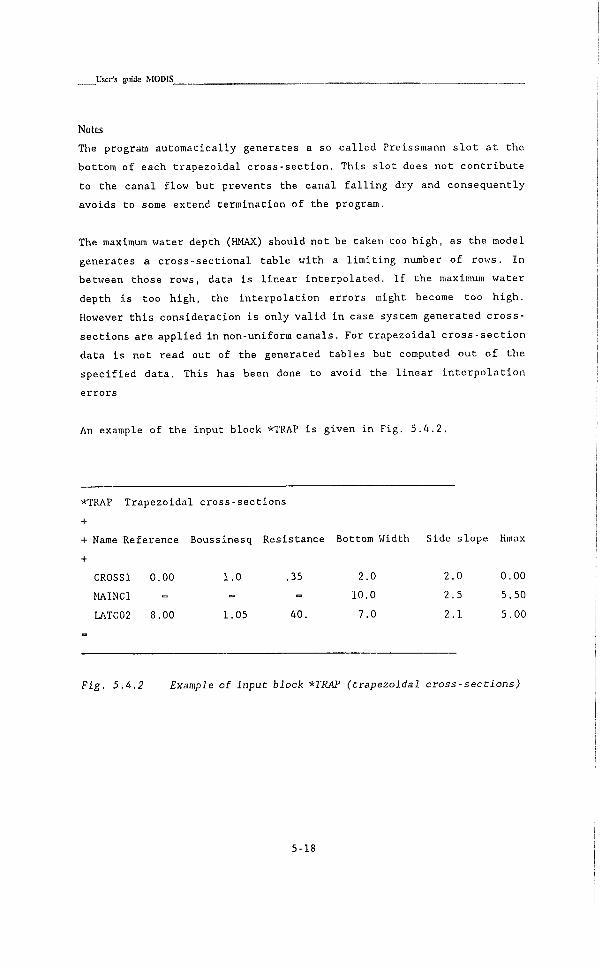
L ' s e r ' s pió^ MODIS_
Note
The program a u t o m a t i c a l l y generates a so c a l l e d Preissmann s l o t a t the
bottom of each t r a p e z o i d a l c r o s s - s e c t i o n . T h i s s l o t does not c o n t r i b u t e
to the c a n a l flow but prevents the c a n a l f a l l i n g dry and c o n s e q u e n t l y
avoids to some extend t e r m i n a t i o n of the program.
The maximum water depth (HMAX) should not be taken too high, as the model
generates a c r o s s - s e c t i o n a l t a b l e w i t h a l i m i t i n g number of rows. I n
between those rows, data i s l i n e a r i n t e r p o l a t e d . I f the maximum water
depth i s too high, the i n t e r p o l a t i o n e r r o r s might become too h i g h .
However t h i s c o n s i d e r a t i o n i s only v a l i d i n case system generated c r o s s -
s e c t i o n s are a p p l i e d i n non-uniform c a n a l s . For t r a p e z o i d a l c r o s s - s e c t i o n
data i s not read out of the generated t a b l e s but computed out of the
s p e c i f i e d data. T h i s has been done to avoid the l i n e a r i n t e r p o l a t i o n
e r r o r s
An example of the input block *TRAP i s given i n F i g . 5.4.2.
*TRAP T r a p e z o i d a l c r o s s - s e c t i o n s
+
+ Name Reference Boussinesq R e s i s t a n c e Bottom Width Side s l o p e Hmax
+
CROSSl 0.00 1.0 .35 2.0 2.0 0.00
MAINCl - - - 10.0 2.5 5.50
LATC02 8.00 1.05 40. 7.0 2.1 5.00
Fig. 5.h.2 Example of Input block •/'TRAP (trapezoidal cross-sections)
5-18
Modd defiilib'ou
S.4.3 Grid - dermition
For the numerical i n t e g r a t i o n of the de S a i n t Venant Equations, a
computational g r i d i s r e q u i r e d aldng each branch. T h i s g r i d i s
a u t o m a t i c a l l y generated by the system f o l l o w i n g the d i r e c t i v e s s e t under
t h i s i n put item and the maximum value f o r Ax s p e c i f i e d i n the branch
input ( s e e paragraph 5.3.2). The system c a l c u l a t e s the number of g r i d
p o i n t s which have to be generated between the u s e r - d e f i n e d g r i d points
i n order to s a t i s f y the c o n d i t i o n on the maximum step s i z e Ax.
The g r i d p o i n t s are a l s o used to l i n k the h y d r a u l i c c a n a l data to the
branches by s p e c i f y i n g f o r each g r i d p o i n t the branch and i t s l o c a t i o n
i n t h a t branch and the name of the c r o s s - s e c t i o n t a b l e .
For each branch a t l e a s t two g r i d points have to be defi n e d by the user:
one a t the beginning and another at the end of the branch. The d e f i n i t i o n
of a d d i t i o n a l g r i d p o i n t s i n between these boundary p o i n t s i s needed only
i f s t r u c t u r e s a re l o c a t e d i n s i d e a branch. I n t h a t case upstream and
downstream of t h a t s t r u c t u r e a d d i t i o n a l g r i d p o i n t s need to be defined.
Of c o u r s e the boundary g r i d p o i n t s can a l s o be used as g r i d points
upstream and downstream of a s t r u c t u r e . However t h i s i s only allowed as
long as the d i s t a n c e between the s t r u c t u r e and the boundary points i s
l i m i t e d , or i f the dynamic behaviour of the branch can be neglected.
The i d e n t i f i c a t i o n l i n e f o r the g r i d d e f i n i t i o n reads a s :
irGRID - DEFINITION OF GRID POINTS
+
+ GRID-POINT CROSS-SECTION BRANCH X-COORDINATE REFERENCE
+ NAME NAME NAME LEVEL
On each subsequent l i n e information about a u s e r - d e f i n e d g r i d point i s
given i n the sequence:
GRID POINT: name of the g r i d p o i n t given by a c h a r a c t e r s t r i n g
f o l l o w i n g the standard convention f o r system element
names
5-19

User's pads MODIS
CROSS-SECTION: name of a c r o s s - s e c t i o n which has been s p e c i f i e d as
d e s c r i b e d i n par. 5.4.1 & 5.4.2;
BRANCH : name of the branch i n which the g r i d point i s l o c a t e d
X-COORDINATE: x- c o o r d i n a t e i n the branch f o r t h i s g r i d p o i n t ;
REFERENCE : r e f e r e n c e l e v e l , g i v i n g the p o s i t i o n of the r e f e r e n c e
l e v e l of the c r o s s - s e c t i o n data w i t h r e s p e c t to the
ge n e r a l model datum l e v e l .
The input of l i n e s does not r e q u i r e a s p e c i a l sequence, n e i t h e r f o r
g i v i n g the in f o r m a t i o n per branch, nor f o r f o l l o w i n g the x - d i r e c t i o n i n
the branch. I t i s , however, a d v i s a b l e to group the data per branch and
separate these groups of l i n e s by blank comment l i n e s .
Note:
The i n t e r p o l a t i o n S I F - c h a r a c t e r " ? " (- i n t e r p o l a t i o n of row data) can
co n v e n i e n t l y be used i n the column f o r c r o s s - s e c t i o n names to i n t e r p o l a t e
the c r o s s - s e c t i o n t a b l e s a t inte r m e d i a t e g r i d p o i n t s . T h i s avoids the
manual c a l c u l a t i o n of such c r o s s - s e c t i o n a l data where an a d d i t i o n a l u s e r -
defined g r i d p o i n t i s introduced merely f o r reasons of, say, output of
r e s u l t s .
I n a d d i t i o n the S I F - c h a r a c t e r " ? " can c o n v e n i e n t l y be used i n the column
for r e f e r e n c e l e v e l , i f the c a n a l has a constant s l o p e . I n F i g . 5.4.3 an
example of the input b l o c k *GRID has been given.
*GRID - DEFINITION OF GRIDPOINTS
+ GRIDPOINT CROSS-SEC BRANCH X-COORDINATE REF LEVEL
G i l CROSSl B l 0 10.00
G12 ? - 500 9.90
G13 ? - 510 9.80
G14 CR0SS2 - 1500 9.75
G21 CR0SS3 B2 0 ?
G22 - - 1250 950
*END OF GRDDEF
Fig- 5.i.i Example of Input block *GRID (grid definition)
5-20

Modd definidon
S.S structures
S.5.1 Introduction
I f s t r u c t u r e s a re placed i n the c a n a l system or i f l a t e r a l i n or outflow
occur, the input segment STRUCTURES should be used. S t r u c t u r e s and
l a t e r a l flow can be placed anywhere i n a branch and should be l o c a t e d i n
between two g r i d p o i n t s . I f s t r u c t u r e s a re p l a c e d i n p a r a l l e l , a l l the
p a r a l l e l l o c a t e d s t r u c t u r e s should be p l a c e d i n between the same g r i d
p o i n t s . I f a t the other hand s t r u c t u r e s a re p l a c e d i n s e r i e s , they should
be s e p a r a t e d by g r i d p o i n t s . The input segment s t r u c t u r e s c o n s i s t s o f
s e v e r a l i n p u t b l o c k s :
*LATQP l a t e r point flows
*WEIR overflow s t r u c t u r e s
*ORIF underflow s t r u c t u r e s
* F I P E pipe s t r u c t u r e s
*PUMP pump s t r u c t u r e s
*LOST l o c a l l o s s s t r u c t u r e s
*NERP Neyrtec module d i s t r i b u t o r s
*FDST f o r t r a n defined s t r u c t u r e s
Each input b l o c k w i l l be d i s c u s s e d subsequently. I f an input block i s not
used, the complete block i n c l u d i n g i t s keyword can be skipped.
The s t r u c t u r e parameters (such as s i l l l e v e l or gate opening h e i g h t ) can
be given e i t h e r as a constant v a l u e or as a f u n c t i o n of an other
parameter. I f the l a t t e r i s used, t h i s f u n c t i o n can be given i n t a b u l a t e d
form, as a f o r t r a n defined f u n c t i o n or as a f u n c t i o n o f an automatic
c o n t r o l l e r .
I f a c o n s t a n t v a l u e i s used, t h i s v a l u e can be given. I n the other c a s e s
a name i s given which r e f e r s to a t a b l e , a f o r t r a n f u n c t i o n or an
automatic c o n t r o l l e r . Automatic c o n t r o l l e r s can only be used f o r the weir
and o r i f i c e type of s t r u c t u r e s . The r e f e r e n c e convention c o n s i s t of four
p a r t s ( T a b l e 5.5.1) :
5-21

L'ser's guide MODIS
1) A one c h a r a c t e r code f o r the type of v a r i a b l e of which the parameter
i s dependent of (e.g T - time, H - upstream water l e v e l ) .
2) A one c h a r a c t e r code f o r the f u n c t i o n type, T f o r t a b u l a t e d
f u n c t i o n s and F f o r f o r t r a n d e f i n e d f u n c t i o n s .
3) A f t e r the two c h a r a c t e r codes s e l e c t e d from the l i s t , the symbol "$"
must be given.
4) F i n a l l y the name of the f u n c t i o n must be given. The name i s l i m i t e d
up to 7 c h a r a c t e r s .
T A B L E 5.5.1 Function references for standard structures except pumps and lateral inflow
Part 1 : code description
T - Time
H - Water l e v e l
Z - C r e s t l e v e l
A - Cross s e c t i o n a l Area of opening
U - Upstream head over the s t r u c t u r e
D - R a t i o downstream/upstream head
0 - Opening h e i g h t of the gate
Y - R a t i o gate opening height/upstream head
L - L o c a l Automatic c o n t r o l
R - Reg i o n a l Automatic c o n t r o l
G - G l o b a l Automatic c o n t r o l (not y e t i n c l u d e d )
PART 2 : Code Description
T - Ta b u l a t e d form
F - F o r t r a n f u n c t i o n
A - Automatic c o n t r o l
PART 3 : $ (dollar sign)
PART 4 : Users defined name, maximum 7 characters
Remark
head i s d e f i n e d as water l e v e l minus c r e s t l e v e l of s i l l .
Automatic c o n t r o l i s only p o s s i b l e i n combination w i t h L o c a l ,
R e g i o n a l or G l o b a l automatic c o n t r o l , e.g. "LA" or "RA".
5-22

Moóé defiüidoD
5.5.2 Laleral discharges
The i d e n t i f i c a t i o n f o r t h i s input item i s given by:
* L A T Q P
+
+ NAME
LATERAL POINT FLOWS AND PUMPS
BRANCH X-COORDINATE DATA TYPE VALUE/REFERENCE
For each l a t e r a l flow source the inf o r m a t i o n i s given on a separate l i n e
under the heading i n the sequence:
SOURCE NAME
BRANCH NAME
X-COORDINATE
DATA TYPE
VALUE
p o i n t source name of maximum 10 c h a r a c t e r s ;
branch name
x-coordinate i n the branch;
C f o r constant v a l u e ;
F f o r a f o r t r a n d e f i n e d f u n c t i o n
TT f o r a t a b u l a t e d f u n c t i o n of time
HT f o r a t a b u l a t e d f u n c t i o n of upstream water l e v e l
AT f o r a t a b u l a t e d f u n c t i o n of c r o s s - s e c t i o n a l area
PT f o r a t a b u l a t e d f u n c t i o n of wetted perimeter
R e a l v a l u e of d i s c h a r g e (m3/s) i f data type i s C
(c o n s t a n t ) and r e f e r e n c e name i f data type i s a (T)
t a b u l a t e d or ( F ) f o r t r a n defined s t r u c t u r e
Note
Remark t h a t for l a t e r a l flow other f u n c t i o n parameters are d e f i n e d than
f o r s t r u c t u r e s as s p e c i f i e d i n Table 5.5.1. The l a t e r a l flows can be
s p e c i f i e d i n random sequence. However, i t i s advised a l s o here to group
them f o l l o w i n g a w e l l organized p a t t e r n as to keep an overview of a l l
data. An example of the input block *LATQP i s given i n F i g . 5.5.1.
5-23

User's guide MODIS
*LATQP- LATERAL POINT FLOWS
+ NAME BRANCH-NAME X-COORD
+
L L I BLB2 15800
LL2 - 48500
LRI BRB 16200
-LRI BRB 16200
LR2 - 43400
TYPE REFERENCE/VALUE
C 5.80
HT HTAB
TT LATQRBI
C 5.20
PT TABl
Fig. 5.5.1 Example of input block *LATQP (lateral point flows)
Tip
With l a t e r a l flow i t i s p o s s i b l e to sim u l a t e c a n a l seepage. I n t h a t case
flow i s s u b t r a c t e d ( n e g a t i v e d i s c h a r g e ) from the c a n a l . The amount of
sub t r a c t e d flow can be given as a ( t a b u l a t e d ) f u n c t i o n of the wetted
perimeter of the c a n a l (DATA TYPE i s PT).
5-24

Modd definidoD
5.5.3 Overflow structures
Introduction
Overflow struct:ures are s t r u c t u r e s whereby the upper water s u r f a c e i s not
touched by the s t r u c t u r e . Both f r e e flow and submerged flow c o n d i t i o n s
can occur and the model s w i t c h e s a u t o m a t i c a l l y to the r i g h t flow
c o n d i t i o n . Furthermore both broad c r e s t e d and sharp c r e s t e d w e i r s can be
modelled. I n p r i n c i p l e , overflow s t r u c t u r e s w i t h any c o n t r o l s e c t i o n can
be modelled, as the exponent u i n the head discharge equation (Eq. 5.1)
i s s p e c i f i e d by the user. As a s p e c i a l f a c i l i t y the s t r u c t u r e can act as
an automatic water l e v e l c o n t r o l s t r u c t u r e . S t r u c t u r e parameters can be
given both for a p o s i t i v e and a n e g a t i v e flow d i r e c t i o n . I f no negative
flow d i r e c t i o n has been s p e c i f i e d the d i s c h a r g e i n the negative d i r e c t i o n
i s assumed to be zero. The a p p l i e d equation f o r overflow s t r u c t u r e s reads
(Bos, 1976):
r e f e r e n c e l e v e l
5.1
IChere
Q - discharge f V s
c, - e f f e c t i v e discharge c o e f f i c i e n t
f - drowned flow r e d u c t i o n f a c t o r
h - upstream water l e v e l head m
b - width of the weir ™
z - c r e s t l e v e l of weir "
u - exponent, normally 1.5
g - a c c e l e r a t i o n due to g r a v i t y
5-25

L'ser's guide MODIS
For more d e t a i l e d I n f o r m a t i o n about overflow s t r u c t u r e s , r e f e r e n c e i s
made to par 11.2.2.
Input data
Under the heading:
*WEIR - overflow s t r u c t u r e
+
+ Name <. .Location. .> <... ..parameters.. . . .>
+ Name Branch X-coor D i r f Ce u B z
The f o l l o w i n g data have to be given i n sequence on each input l i n e :
NAME : Name of the s t r u c t u r e (maximum 10 c h a r a c t e r s ) . For each
s t r u c t u r e a new name has to be s p e c i f i e d .
BRANCH : Branch name i n which the s t r u c t u r e i s l o c a t e d .
X-COOR : P o s i t i o n along the x - a x i s i n the branch.
DIR : Flow d i r e c t i o n f o r which the s t r u c t u r e parameters are
used. T h i s i s s p e c i f i e d by a s t r i n g of two c h a r a c t e r s :
PX : f o r flow i n p o s i t i v e x - d i r e c t i o n through the
s t r u c t u r e .
NX : f o r flow i n negative x - d i r e c t i o n through the
s t r u c t u r e .
F : Drowned flow r e d u c t i o n f a c t o r . I f the flow through the
s t r u c t u r e i s always modular ( f r e e f l o w ) , a v a l u e of 1.0
can be give n .
CE : E f f e c t i v e d i s c h a r g e c o e f f i c i e n t .
U : The power used i n the w e i r flow equation. Normally a va l u e
of 1.5 i s used. For non r e c t a n g u l a r c o n t r o l s e c t i o n s other
v a l u e s may occur.
B : Width of c o n t r o l s e c t i o n of the weir.
Z : S i l l l e v e l of the weir.
I f a l l s t r u c t u r e s have been defined, the input segment i s c l o s e d by a
l i n e w i t h the symbol "-" i n the f i r s t column.
5-26

ModfcJ dfcfvmdon
Notes
A smooth t r a n s i t i o n between f r e e and submerged flow can be ach i e v e d
by s p e c i f y i n g the v a l u e of the drowned flow r e d u c t i o n f a c t o r f as a
f u n c t i o n of the r a t i o between the downstream and upstream head e.g.
DT$FRED (see T a b l e 5.5.1 and F i g 11.2.2).
( h 2 - z ) / ( h l - z ) FRED
0.00 1.00
0.67 1.00
0.80 0.75
0.90 0.55
1.00 0.00
The same procedure can be adapted f o r s p e c i f y i n g the e f f e c t i v e
d i s c h a r g e c o e f f i c i e n t Ce. By g i v i n g the va l u e of Ce as a f u n c t i o n of
the upstream head (e.g. UT$CE), the t r a n s i t i o n from a sharp to a
broad c r e s t e d w e i r can be simulated.
Automatic c o n t r o l of an overflow s t r u c t u r e by means of c o n t r o l l e r s
i s p o s s i b l e . E i t h e r the parameter B or Z can be a u t o m a t i c a l l y
a d j u s t e d i n order to keep a constant water l e v e l somewhere i n the
c a n a l system. I n t h a t case r e f e r e n c e i s made to input segment
automatic c o n t r o l , u s i n g the standard f u n c t i o n r e f e r e n c e (e.g.
LA$C0NTR or RA$C0NTR, paragraph 5.6).
Sometimes i t i s needed to use the energy head H, i n s t e a d of the
water l e v e l h i n Eq. 5.1. T h i s can be ach i e v e d by s p e c i f y i n g an
a d d i t i o n a l g r i d p o i n t c l o s e to the s t r u c t u r e w i t h a Bou s s i n e s q
c o e f f i c i e n t ^ of the upstream c r o s s - s e c t i o n equal to z e r o . I n t h a t
way the v e l o c i t y head i s transformed i n t o a s t a t i c head [Rubicon,
1984] .
An example of the input segment *WEIR i s given i n F i g . 5.5.2
5-27

User's guide MODIS_
*WEIR - overflow s t r u c t u r e
+ Name <. .Location. .> <... ..parameters.. ...>
+ NAME BRANCH X-COOR DIR F Ce u B Z
Wl B2 950 PX DT$FRED UT$CE 1.5 2 4.0
Wl - - N X - _ _ _ _
REG B8 375 PX 1 0.9 1.5 6 LA$C0NTR1
Fig. 5.5.2 Example of input segment *WEIR (overflow structures)
Notes:
The s t r u c t u r e Wl can flow i n two d i r e c t i o n s . The s i l l h e i g h t of the
s t r u c t u r e REG i s a u t o m a t i c a l l y a d j u s t e d (LA$C0NTR). A l l f u n c t i o n s
and c o n t r o l l e r s have to be s p e c i f i e d l a t e r .
5-28

Modd definidoa
5.5.4 Orifice structures
Introduction
Underflow s t r u c t u r e s a re s t r u c t u r e s whereby the upper flow surface i s
touched by the s t r u c t u r e gate. However, i f the upstream head becomes too
low the o r i f i c e s t r u c t u r e w i l l a u t o m a t i c a l l y a c t as a ( f r e e or submerged)
weir.
Under the heading "*ORIF" underflow s t r u c t u r e s are grouped. The input
segment f o r underflow s t r u c t u r e s i s v e r y much the same as for overflow
s t r u c t u r e s . The equation f o r both f r e e and submerged, o r i f i c e flow with
a r e c t a n g u l a r c o n t r o l s e c t i o n and v a r i a b l e gate opening reads;
UlKu ;iiiiiil;iiiii:iiiiiiiitii;i!i:tiiiiii!i::iiiui;ii
energy l e v e l
'i3lliiini:iiiiilill;ijiiiiiilii!iiiiil:ilill
r e f e r e n c e l e v e l
Q = c^fiby 'Jlglh
Where
Q -
Co -
b
y
dh -
g
d i s c h a r g e
e f f e c t i v e d i s c h a r g e c o e f f i c i e n t
opening c o n t r a c t i o n c o e f f i c i e n t (0.63)
width of c o n t r o l s e c t i o n
opening h e i g h t of gate
head d i f f e r e n c e ,
a c c e l e r a t i o n of g r a v i t y
5.2
m'/s
m
m
ra
m/s2
I f the downstream water l e v e l does not e f f e c t the disc h a r g e (modular
flow) the head d i f f e r e n c e (dh) becomes;
5-29
L W s guide MODIS_
i h - hi - (z + tiy) 5.3
Where
z s i l l l e v e l m
y
opening c o n t r a c t i o n c o e f f i c i e n t
gate opening h e i g h t . m
I f the flow i s submerged, the head d i f f e r e n c e (dh) i s equal to:
Ah - h 5.4 1
Where hj and h2 are the upstream and downstream water l e v e l s r e s p e c t i v e l y .
The u s e r can s p e c i f y i f the flow becomes submerged. This i s done by u s i n g
a flow f a c t o r f, which can be s p e c i f i e d as a fun c t i o n of upstream and
downstream water l e v e l head and gate opening height. (Beware t h a t t h i s
f a c t o r f i s not the same as the drowned flow r e d u c t i o n f a c t o r of the we i r
formula p r e s e n t e d i n Equation 5.1).
Input
Under the heading:
•*ORIF - underflow s t r u c t u r e
+ Name <. .Location. .> <... ..parameters.. ...>
+ NAME BRANCH X-COOR DIR F Ce U B Z Y
The f o l l o w i n g data has to given i n sequence i n each input l i n e :
NAME : Name of the s t r u c t u r e (maximum 10 c h a r a c t e r s ) . For each
s t r u c t u r e an unique name must be given.
BRANCH : Branch name i n which the s t r u c t u r e i s l o c a t e d .
X-COOR : P o s i t i o n along the x - a x i s i n the branch.
DIRECTION : Flow d i r e c t i o n f o r which the s t r u c t u r e parameters are
used. The flow d i r e c t i o n can be e i t h e r :
PX f o r flow i n p o s i t i v e x - d i r e c t i o n through the
s t r u c t u r e .
NX f o r flow i n n e g a t i v e x - d i r e c t i o n through the
5-30
Model definitioü
Ce
U
B
Z
Y
s t r u c t u r e .
Drovmed flow c o e f f i c i e n t which v a l u e i s i n between 0 and
1. I f the flow through the s t r u c t u r e i s always submerged
f should be equal to one. I f a t the other hand there i s
always f r e e flow, f should be equal to zero.
E f f e c t i v e discharge c o e f f i c i e n t .
Opening c o n t r a c t i o n c o e f f i c i e n t (= 0.63).
Width of c o n t r o l s e c t i o n .
S i l l l e v e l .
Opening height of the gate
I f a l l s t r u c t u r e s have been defined, t h i s i n put segment i s c l o s e d by a
l i n e w i t h the symbol "-" i n the f i r s t column.
Notes
Beware t h a t the F - c o e f f i c i e n t f o r o r i f i c e s t r u c t u r e s i s d i f f e r e n t from
the drowned flow r e d u c t i o n c o e f f i c i e n t used i n overflow s t r u c t u r e s ! The
computer model checks which type of flow i s a p p l i c a b l e by comparing the
a c t u a l r a t i o of the gate opening h e i g h t and the downstream head with the
v a l u e of f. I f the a c t u a l r a t i o i s higher than the v a l u e of f, modular
flow i s assumed (see paragraph 11.2.3). The f a c t o r f can be given as a
c o n s t a n t value or as a f u n c t i o n of the r a t i o gate opening h e i g h t and
upstream water l e v e l head YT$FCOEF. For example:
h2-z/y FCOEF
0.000 0.000
0.001 0.002
0.100 0.227
0.125 0.256
0.143 0.270
0.166 0.300
0.200 0.333
0.250 0.377
0.333 0.456
0.500 0.588
0.667 0.770
1.000 1.000
5-31

L W s guide MODIS_
I f the downstream water l e v e l i s below the gate opening h e i g h t and the
upstream head becomes l e s s than 1.5 times the gate opening h e i g h t , the
s t r u c t u r e w i l l a c t as a ( f r e e or submerged) weir w i t h a c, c o e f f i c i e n t of
1.0.
The c o n t r a c t i o n c o e f f i c i e n t can be given as a constant or as a f u n c t i o n
of the gate opening h e i g h t and upstream head e.g. YT$CNTRAC.
The o r i f i c e can a c t as an automatic c o n t r o l l e d water l e v e l r e g u l a t o r by
making r e f e r e n c e to the automatic c o n t r o l l e r s i n s t e a d of g i v i n g a va l u e
f o r the gate opening hei g h t .
An example of the input segment *0RIF i s given i n F i g . 5.5.3
*0RIF - underflow s t r u c t u r e
+
+ Name <. .Location. .> <...
+ NAME BRANCH X-COOR DIR F
+
GATEl B2 950 PX YT$FC0EF
- - NX 0.0
ORIF B8 375 PX 1.0
..parameters. . . . .>
CE U B Z Y
0.8 0.63 2.0 11.20 RA$CNTR
0.0 - _ _
0.9 0.70 6 10.20 TT$0P1
Fig. 5.5.3 Example of input segment *ORIF (orifice structures)
5-32

S.5.S Pipe structures
Introduction
Pipe s t r u c t u r e s can be used to model flow through pipe o f f t a k e s and
h o r i z o n t a l c u l v e r t s . The c h a r a c t e r i s t i c s of pipe flow are complicated.
S e v e r a l flow c o n d i t i o n s may occur, whereby the pipe can be completely or
p a r t l y f i l l e d . I n p r i n c i p l e , h y d r a u l i c long c u l v e r t s can be modelled
only. I n case of h y d r a u l i c s h o r t c u l v e r t s , whereby the c u l v e r t i s p a r t l y
f i l l e d and a c t s as an o r i f i c e , the user i s a d v i s e d to model the c u l v e r t
as an o r i f i c e s t r u c t u r e . [Ven te Chow, 1959). I f the pipe i s completely
f i l l e d , submerged flow, f r e e flow and a e r a t e d f r e e flow can occur. The
pipe w i l l a c t as a weir i f the downstream l e v e l i s below the top of the
pipe opening and i f the upstream water l e v e l i s below a c r i t i c a l l e v e l .
T h i s c r i t i c a l l e v e l can be s p e c i f i e d by the u s e r and normally v a r i e s
between 1.5 and 1.2 times the pipe diameter.
The g e n e r a l equation f o r f u l l p i p e flow reads:
Q = . J _ Ay/Zgth 5.5
Where
Q - discharge m'/s
c^ - t o t a l l o s s c o e f f i c i e n t , c o n s i s t i n g of entrance, f r i c t i o n and
e x i t l o s s e s
A - c r o s s - s e c t i o n a l area of gate opening
dh - head d i f f e r e n c e . ni
5-33
L'ser's guide MODIS
The head d i f f e r e n c e (dh) depends on the flow c o n d i t i o n . Three flow
c o n d i t i o n s a re d i s t i n g u i s h e d :
aerated flow
I f the downstream water l e v e l i s below the bottom l e v e l of the opening,
the flow i s f u l l y a e r a t e d and dh becomes:
Ah » hi - ^ (h,-\„,,<^) 5.6
VThere hi i s the upstream water l e v e l , ht^p i s the top of opening and htottom
i s the bottom l e v e l of the pipe.
modular flow
I f the downstream water i s above the bottom l e v e l and below the top of
opening dh becomes:
A h » h i - h , 115.7
submerged flow
I f the downstream water l e v e l i s above the top l e v e l of opening, the flow
i s submerged and dh becomes:
i h - hi - h j 5.8
Where hj i s the downstream water l e v e l .
Partly filled pipe flow
I f the downstream water l e v e l i s below the top of opening of the pipe,
the pipe can be p a r t l y f i l l e d , depending on the upstream water l e v e l . I f
the upstream water l e v e l i s above a c r i t i c a l l e v e l , the pipe i s assumed
to be completely f i l l e d . The c r i t i c a l l e v e l i s equal to :
^ c r i t i c a l " ^ b o t t o m * (^T " b o t t o m ) ' ̂
5-34

Modd definition
Whereby t:he f a c t o r f i s s p e c i f i e d by the user. Normally f v a r i e s between
1.5 and 1.2, the l a t t e r for longer pipe l e n g t h s .
I f the upstream water l e v e l i s below the c r i t i c a l l e v e l the pipe w i l l be
p a r t l y f i l l e d and the weir flow equation i s a p p l i e d . The flow can be
e i t h e r f r e e or submerged depending on the r a t i o of the upstream and
downstream head. I f the downstream head i s l e s s than 2/3 of the upstream
head, f r e e w e i r flow i s assumed:
" t " ' ' b o t t o m
I f the downstream head i s g r e a t e r than 2/3 of the upstream head, drowned
we i r flow w i l l be assumed:
Q - ( ' l 2 - ' \ o t t o n n ) / 2 i ; ^ 5.11
" t ~ " b o t t o m
T h e loss coef f i c ien t
The l o s s c o e f f i c i e n t c, c o n s i s t of :
-entrance l o s s c o e f f i c i e n t
c . f 1 - 1^2 5.12 '-entrance — '
- r e s i s t a n c e l o s s c o e f f i c i e n t
c - 5.13 ' - r e s i s t a n c . 'pr^fTl
- e x i t l o s s c o e f f i c i e n t (1.0)
5.14
Where, R - h y d r a u l i c r a d i u s of pipe (- A/jrD) , D - diameter of pipe, k -
S t r i c k l e r r e s i s t a n c e c o e f f i c i e n t and L - length of pipe.
5-35

Input
Under the heading:
*PIPE - pipe s t r u c t u r e
+
+ <. .LOCATION. .> <...
+ NAME BRANCH X-COOR DIR F
..PARAMETERS.. . . .>
Ct A Hbottom Htop
The f o l l o w i n g data has to given:
NAME
BRANCH
X-COOR
DIRECTION
Ct
A
Hbottom
Htop
Name of the s t r u c t u r e (maximum 10 c h a r a c t e r s ) .
Branch name i n which the s t r u c t u r e i s l o c a t e d .
P o s i t i o n along the x - a x i s i n the branch.
Flow d i r e c t i o n f o r which the s t r u c t u r e parameters a re
used. The flow d i r e c t i o n can be e i t h e r :
PX : f o r flow i n p o s i t i v e x - d i r e c t i o n through the
s t r u c t u r e .
NX : for flow i n negative x - d i r e c t i o n through che
s t r u c t u r e .
F - c o e f f i c i e n t s p e c i f i e s the c r i t i c a l l e v e l below which
w e i r flow w i l l occur. The val u e of f i s nor m a l l y i n
between 1.0 and 1.5.
T o t a l l o s s c o e f f i c i e n t .
C r o s s - s e c t i o n a l a r e a of pipe opening.
Bottom l e v e l of opening.
Top l e v e l of opening
5-36
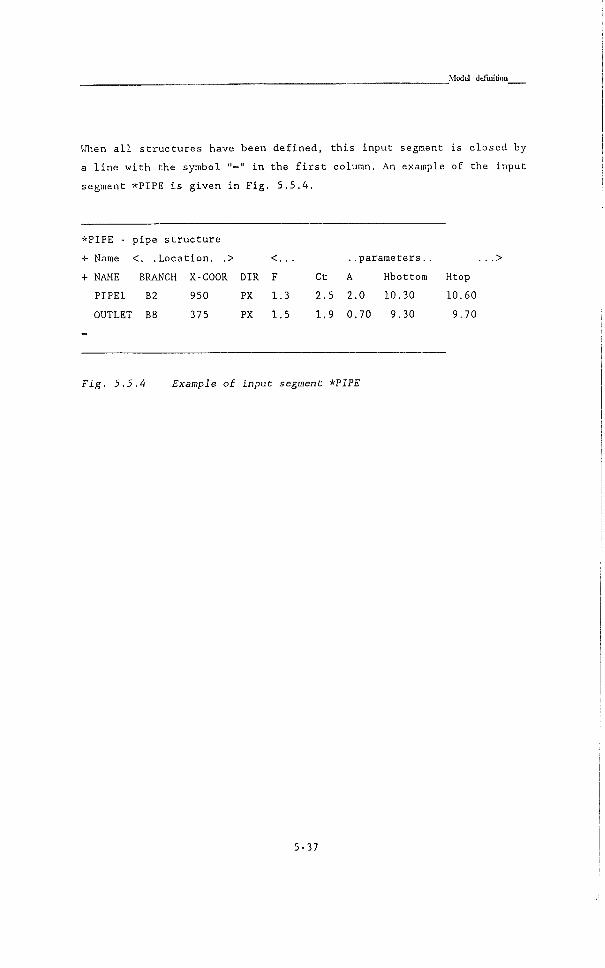
Model definition
When a l l stzructures have been defined, t h i s input segment i s c l o s e d by
a l i n e w i t h the symbol "-" i n the f i r s t column. An example of the input
segment * P I P E i s gi v e n i n F i g . 5.5.4.
*PIPE - pipe s t r u c t u r e
+ Name <. .Loca t i o n . .> <... ..parameters.. ...>
+ NAME BRANCH X-COOR DIR F Ct A Hbottom Htop
P I P E l B2 950 PX 1.3 2.5 2.0 10.30 10.60
OUTLET B8 375 PX 1.5 1.9 0.70 9.30 9.70
Fig. 5.5.4 Example of input: segmenC *PIPE
5-37
L W s guide MODIS_
5.5.6 Pump structures
Introduction
Pump s t r u c t u r e s are non g r a v i t y flow s t r u c t u r e s whicti i m p l i e s that the
flow through the pump s t r u c t u r e i s not i n f l u e n c e d by the upstream and
downstream water l e v e l s , but the d i s c h a r g e i s p r e - d e s c r i b e d by the user.
Operation of the pump i s c o n t r o l l e d by s p e c i f y i n g a s t a r t and stop water
l e v e l . Pump o p e r a t i o n i s s t a r t e d i f the a c t u a l water l e v e l exceeds the
s t a r t l e v e l and pump ope r a t i o n i s stopped i f the a c t u a l water l e v e l drops
below the stop l e v e l . The stop water l e v e l should always be below the
s t a r t water l e v e l i n order to avoid too frequent on and o f f s w i t c h i n g .
I f a pump s t a t i o n c o n s i s t i n g of s e v e r a l pumps with d i f f e r e n t s t a r t and
stop water l e v e l s need to be modelled, the user i s ad v i s e d to model
s e v e r a l pumps wi t h d i f f e r e n t names but on the same l o c a t i o n , each one
with i t s own s t a r t and stop l e v e l s .
Input
Under the heading
*PUMP - pump s t r u c t u r e s
+
+ NAME BRANCH X-COOR DIR F CAPACITY H-START H-STOP
The f o l l o w i n g data has to be given:
NAME
BRANCH
X-COOR
DIR
CAPACITY
Name of the pump s t r u c t u r e
Branch name i n which the s t r u c t u r e i s l o c a t e d
P o s i t i o n along the x - a x i s
Water l e v e l which c o n t r o l s pump opera t i o n :
PX - Upstream water l e v e l
NX - Downstream water l e v e l
Reduction f a c t o r of pump c a p a c i t y , can be given e.g. as a
ta b u l a t e d f u n c t i o n of the head.
C a p a c i t y or disch a r g e of Che pump i f che pump i s i n
op e r a t i o n
5-38

Modd defmib'uu
H-START : Water l e v e l above which pump i s turned on
H-STOP : Water l e v e l below which pump i s turned o f f
I f a l l pump s t r u c t u r e s have been defined, t h i s input segment i s c l o s e d
by a l i n e w i t h the symbol "-" i n the f i r s t column.
Example
An example of t h i s input block i s given i n F i g . 5.5.5
*PUMP - pump s t r u c t u r e s
+
+ NAME BRANCH X-COOR DIR
PUMPl BRANCH3 2000 PX
PUMP2 BRANCH3 2000 PX
F CAPACITY H-START H-STOP
HT$HEAD 2.50 10.A5 10.35
HT$HEAD 1.50 10.55 10.A5
Fig. 5.5.5 Example of input segment *PUMP
5-39

User's guide MODIS_
5.5.7 Local loss structures
Introduction
L o c a l l o s s s t r u c t u r e s are f r e q u e n t l y found along i r r i g a t i o n c a n a l s .
Example of l o c a l l o s s s t r u c t u r e s are bridges and c u l v e r t s but a l s o abrupt
p r o f i l e changes. The input segment f o r l o c a l l o s s s t r u c t u r e s i s v e r y much
the same as the d e f i n i t i o n of other type of s t r u c t u r e s .
The head l o s s due to abrupt p r o f i l e changes can be computed u s i n g the
formulae:
Ah-ci^ v l i l !
w h i l e the head l o s s of a l o s s s t r u c t u r e s can be computed u s i n g the
formulae:
5.16
Where
dh - head l o s s
c - l o s s c o e f f i c i e n t
Vj - flow v e l o c i t y a t the vena
Vj - flow v e l o c i t y downstream
m
c o n t r a c t a ra/s
m/s
Input
Under the heading:
*LOST - l o c a l l o s s s t r u c t u r e s
+
+ Name <. .Location. .> <.. parameters.. >
+ Name Branch X-coor Type D i r C A
The f o l l o w i n g data has to be given;
NAME : Name of the s t r u c t u r e (maximum 10 c h a r a c t e r s ) .
BRANCH : Branch name i n which the s t r u c t u r e i s lo c a t e d .
X-COOR : P o s i t i o n along the x - a x i s i n the branch,
5-40
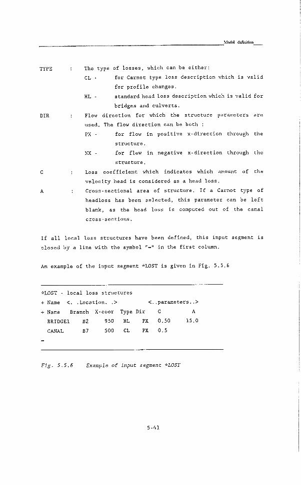
Model delimtion
TYPE : The type of l o s s e s , which can be e i t h e r :
CL - f o r Carnot type l o s s d e s c r i p t i o n which i s v a l i d
for p r o f i l e changes.
HL - standard head l o s s d e s c r i p t i o n which i s v a l i d f o r
bridges and c u l v e r t s .
DIR : Flow d i r e c t i o n f o r which the s t r u c t u r e parameters a r e
used. The flow d i r e c t i o n can be both :
PX - f o r flow i n p o s i t i v e x - d i r e c t i o n through the
s t r u c t u r e .
NX - f o r flow i n negative x - d i r e c t i o n through the
s t r u c t u r e .
C : Loss c o e f f i c i e n t which i n d i c a t e s which amount of the
v e l o c i t y head i s c o n s i d e r e d as a head l o s s .
A : C r o s s - s e c t i o n a l a r e a of s t r u c t u r e . I f a Carnot type of
h e a d l e s s has been s e l e c t e d , t h i s parameter can be l e f t
blank, as the head l o s s i s computed out of the c a n a l
c r o s s - s e c t i o n s .
I f a l l l o c a l l o s s s t r u c t u r e s have been defined, t h i s input segment i s
c l o s e d by a l i n e w i t h the symbol "-" i n the f i r s t column.
An example of the input segment *LOST i s given i n F i g . 5.5.6
*LOST - l o c a l l o s s s t r u c t u r e s
+ Name <• .Location. .> <..parameters..>
+ Name Branch X-coor Type D i r C A
BRIDGEl B2 950 HL PX 0.50 15.0
CANAL B7 500 CL PX 0.5
Fig. 5.5.6 Example of input segment *LOST
5-41
L W s guUe MODIS_
5.5.8 Neyrtec distributors
Introduction
Neyrtec d i s t r i b u t o r s a re s p e c i a l o f f t a k e s t r u c t u r e s , which a r e able to
maintain a n e a r l y c o n s t a n t d i s c h a r g e w h i l e the upstream water l e v e l
v a r i e s w i t h i n a c e r t a i n range. The Neyrtec d i s t r i b u t o r s a c t as a
combination of w e i r and o r i f i c e s t r u c t u r e w i t h a h i g h l y v a r i a b l e
c o n t r a c t i o n c o e f f i c i e n t . I n the computer model s t a n d a r d t a b l e s have been
included i n which the di s c h a r g e as a f u n c t i o n of the upstream water l e v e l
has been t a b u l a t e d .
Input
Under the heading:
*NERP
+ Name Branch X Type X d i r B Z
+
The f o l l o w i n g data has to be given:
NAME : Name of the s t r u c t u r e (maximum 10 c h a r a c t e r s ) .
BRANCH : Branch name i n which the s t r u c t u r e i s l o c a t e d .
X-COOR : P o s i t i o n along the x - a x i s i n the branch.
TYPE : One of the types of Table 5.5-2 can be s e l e c t e d . (The
a p p l i e d n o t a t i o n i s s i m i l a r to the n o t a t i o n of Neyrtec,
which produces the modules).
X d i r : PX f o r p o s i t i v e flow d i r e c t i o n .
NX f o r negative flow d i r e c t i o n .
B : The e f f e c t i v e width of the module. The e f f e c t i v e width i s
somewhat l e s s than the t o t a l width. Example, a r e a l l ength
of 0.32 m (Type :X1) has an e f f e c t i v e l e n g t h of 0.30 m as
the nominal d i s c h a r g e i s 0.30 m * 100 1/s/m = 30 1/s.
Z ; S i l l l e v e l of the module. I n Table 5.5-2 the de s i g n heads
of the modules are given. I d e a l l y the s i l l l e v e l should be
equal to the designed water l e v e l minus the de s i g n head.
5-42
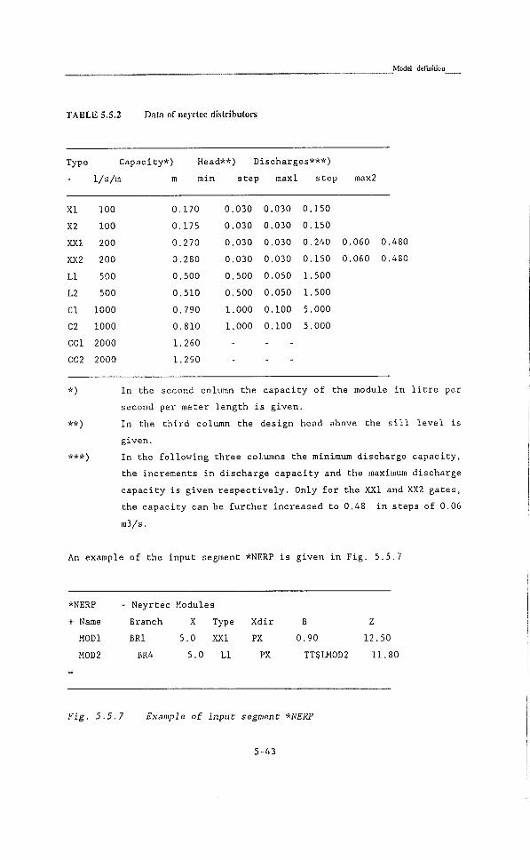
Modd definidon
T A B L E 5.5.2 D a t a o f neyr tec d i s t r i bu to r s
Type C a p a c i t y * ) Head**) D i s c h a r g e s * * * )
- 1/s/m m min step maxl step raax2
XI 100 0. 170 0, 030 0. 030 0. 150
X2 100 0. 175 0, ,030 0, 030 0. 150
XXI 200 0. 270 0, ,030 0, ,030 0, 240 0.060 0.
XX2 200 0. ,280 0, .030 0, ,030 0. ,150 0.060 0.
L l 500 0, ,500 0, ,500 0, ,050 1, ,500
L2 500 0, ,510 0 ,500 0, .050 1, ,500
C l 1000 0 .790 1 .000 0 .100 5, ,000
C2 1000 0 .810 1 .000 0 .100 5, ,000
CCI 2000 1 .260 - -
CC2 2000 1 .290 - -
*) I n the second column the c a p a c i t y of the module i n l i t r e per
second per meter length i s given.
**) I n the t h i r d column the design head above the s i l l l e v e l i s
given.
***) I n the f o l l o w i n g three columns the minimum disc h a r g e c a p a c i t y ,
the increments i n disc h a r g e c a p a c i t y and the maximum discharge
c a p a c i t y i s g i v e n r e s p e c t i v e l y . Only f o r the XXI and XX2 gates,
the c a p a c i t y can be f u r t h e r i n c r e a s e d to 0.48 i n steps of 0.06
m3/s.
An example of the input segment *NERP i s given i n F i g . 5.5.7
*NERF - Neyrtec Modules
+ Name Branch X Type
MODI BRI 5.0 XXI
M0D2 BR4 5.0 L l
X d i r B Z
PX 0.90 12.50
PX TT$LM0D2 11.80
Fig. 5.5.7 Example of input: segment *NERF
5-43

User's guide MODIS
Note Operation of the n e y r t e c d i s t r i b u t o r s can be simulated by s p e c i f y i n g
the width of the s i l l as a t a b u l a t e d f u n c t i o n of time f o r example.
5-A4

Modei dfcfiiiiüou
S.5.9 Fortran defined function
Introduction
I f a s t r u c t u r e can not be d e s c r i b e d by one of the stan d a r d s t r u c t u r e s ,
t h i s s t r u c t u r e can s t i l l be inc l u d e d i n the model, namely as a F o r t r a n
d e f i n e d s t r u c t u r e . Before u s i n g t h i s f a c i l i t y however, the us e r i s
ad v i s e d to convince h i m s e l f t h a t i t i s imp o s s i b l e to make use of one of
the s t a n d a r d s t r u c t u r e , as n e a r l y a l l s t r u c t u r e s can be r e w r i t t e n as one
of the gi v e n standard s t r u c t u r e s . A f o r t r a n d e f i n e d s t r u c t u r e i s somewhat
more co m p l i c a t e d than the other s t r u c t u r e s , as the us e r has to w r i t e a
f o r t r a n subroutine and l i n k t h i s subroutine to the model. I f a f o r t r a n
d e f i n e d s t r u c t u r e i s used the f o l l o w i n g data have to be given i n the
model d e f i n i t i o n .
Input
Under the heading:
*FDST
+ NAME BRANCH X
the u s e r g i v e s on each input l i n e the f o l l o w i n g data :
NAME : name of f o r t r a n s t r u c t u r e (max 10 c h a r a c t e r s )
BRANCH : the branch i n which the s t r u c t u r e i s p o s i t i o n e d
X-COOR : P o s i t i o n along the x - a x i s i n the branch.
The i n p u t b l o c k i s c l o s e d by l i n e c o n t a i n i n g the symbol "=" i n the f i r s t
column.
Writing a fortran function
To i n c l u d e a f o r t r a n d e f i n e d f u n c t i o n the f o l l o w i n g procedure has to be
followed.
1) Give the r e q u i r e d input data as d i s c u s s e d above.
2) Write the f o r t r a n f u n c t i o n i n FORTRAN 77 computer language.
3) Change the source code of F o r t r a n subroutine FSTRUC, l o c a t e d i n
f i l e MODCOMXF.FOR.
4) Compile both the newly w r i t t e n f o r t r a n f u n c t i o n and FSTRUC wi t h
5-45
L W s guide MODIS_
a p r o f e s s i o n a l F o r t r a n Compiler.
5) L i n k the whole subsystem MODCOM again.
ad 1) The name given i n the input block r e f e r s to a F o r t r a n - d e f i n e d
f u n c t i o n which has to be w r i t t e n by the user and then must be
compiled and l i n k e d to the subsystem MODCOM.
ad 2) The f o r t r a n program should s t a r t w i t h the heading
FUNCTION CULVERT (I,H1,H2)
where the v a r i a b l e s r e p r e s e n t :
I ; s t r u c t u r e number
HI : water l e v e l a t the upstream g r i d p o i n t .
H2 : water l e v e l a t the downstream g r i d p o i n t .
Then the body of the program can be w r i t t e n . An example o f such
a program i s gi v e n i n F i g . 5.5.7
ad 3) Read MODCOMXF.FOR i n an e d i t o r . I n the subprogram FSTRUC i t i s
al r e a d y i n d i c a t e d where to change the source code. The only
t h i n g the user has to do i s to change the name of CULVERT i n to
the new name.
ad 4) Compiling the programs i s q u i t simple. I f one i s us i n g RMFORT-
corapiler the commando should read:
RMFORT MODCOMXF /Z <ENTER>
I f the M i c r o s o f t f o r t r a n compiler i s used the commando should
read:
F L /c MODCOMXF.FOR followed by p r e s s i n g <ENTER>
I f no e r r o r messages are given one can continue, otherwise the
program(s) should be made e r r o r f r e e .
ad 5) F i n a l l y the complete program can be l i n k e d again: COMLNK
<enter> Now the new w r i t t e n program i s i n c l u d e d i n MODCOM.EXE
5-46
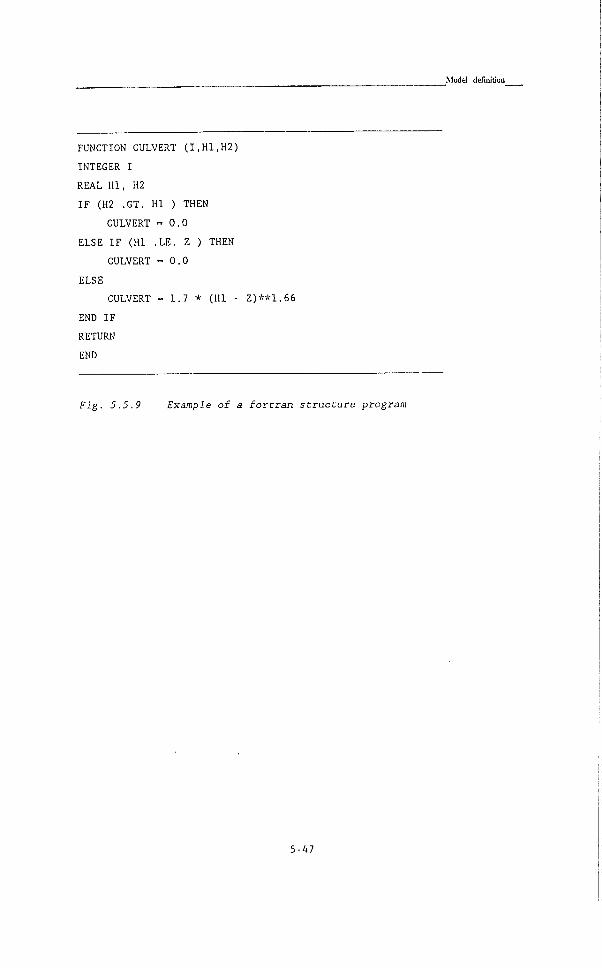
Modd defiüidoQ
FUNCTION CULVERT (I,H1,H2)
INTEGER I
REAL HI, H2
I F (H2 .GT. HI ) THEN
CULVERT - 0.0
ELSE I F (HI .LE. Z ) THEN
CULVERT - 0.0
ELSE
CULVERT - 1.7 * (HI - Z)**1.66
END I F
RETURN
END
Fig. 5.5.9 Example of a foreran structure program
5-A7

User's guide MODIS_
5.6 Automatic control systems
5 .6 .1 I n t r o d u c t i o n
I n the computer model v a r i o u s automatic c o n t r o l l e r s are i n c o r p o r a t e d
which can be used to c o n t r o l w e i r or o r i f i c e s t r u c t u r e s . One can s e l e c t
between t h r e e l e v e l s of c o n t r o l , namely: l o c a l , r e g i o n a l and g l o b a l
c o n t r o l . Furthermore e i t h e r step- or F I D - c o n t r o l l e r s can be used.
The output s i g n a l of a P I D - c o n t r o l l e r reads:
" t - Zo * ̂ i 5 2 e ^ + (e^-e^.i) 5.17
The output s i g n a l of a step c o n t r o l l e r i s computed by:
u, - Uf + V i t 5.18
For r e g i o n a l c o n t r o l , the output s i g n a l can a l s o be computed according
to CARDD-control or B I V A L - c o n t r o l l e r . The l a t t e r i s very much the same
as a step c o n t r o l l e r , whereby the t a r g e t l e v e l i s v a r i e d a c c o r d i n g to the
f o l l o w i n g formula:
V . y n QmaxJ^Qpivot 5.19 ^target 'target,Q_ + ̂ q
Where
ut - output s i g n a l
y - t a r g e t l e v e l
D - dead band
zO - c o n s t a n t (parm2)
Kp - p r o p o r t i o n a l g a i n f a c t o r
K i - i n t e g r a l gain f a c t o r
Kd - d i f f e r e n t i a l g a i n f a c t o r
V - speed of gate movement (meters/minute)
e t - d e v i a t i o n from s e t - p o i n t (- t a r g e t l e v e l - a c t u a l l e v e l )
Maximum d i s c h a r g e a t p i v o t p o i n t
For more in f o r m a t i o n about the c o n t r o l l e r s and the determination of v a l u e
of the c o n t r o l parameters, p l e a s e r e f e r to par. 11.3.4. With che help of
5-48

Model defijiidüu
the automatic c o n t r o l f a c i l i t y v a r i o u s c o n t r o l systems can be implemented
i n MODIS such as automatic upstream and dovmstream c o n t r o l , B i v a l
c o n t r o l , c o n s t a n t volume c o n t r o l e t c e t e r a . The c o n t r o l l e r computes every
s i m u l a t i o n step an output s i g n a l based on a c t u a l water l e v e l
measurements. T h i s output s i g n a l i s used to determine f o r example a new
s i l l l e v e l or a gate opening h e i g h t i n order to ma i n t a i n a con s t a n t l e v e l
somewhere i n the system.
To use the automatic c o n t r o l f a c i l i t y the user has to s p e c i f y by the
d e f i n i t i o n of the s t r u c t u r e s , a name f o r the c o n t r o l l e r i n s t e a d of a
s t r u c t u r e parameter. (Maximum t o t a l length of the r e f e r e n c e i s 10
c h a r a c t e r s e.g. LA$C0NTR1 whereby "LA" i n d i c a t e s L o c a l Automatic c o n t r o l ,
"$" i s a s e p a r a t i o n s i g n and CONTRl i s a u s e r s s p e c i f i e d name). The name
"CONTRl" r e f e r s to the automatic c o n t r o l input segment which w i l l be
d i s c u s s e d h e r e .
The i n p u t segment automatic c o n t r o l c o n s i s t s of three input b l o c k s
*AULC - automatic l o c a l c o n t r o l
*AURC - automatic r e g i o n a l c o n t r o l
*AUGC - automatic g l o b a l c o n t r o l
5.6.2 Automatic local control
Automatic l o c a l c o n t r o l i m p l i e s t h a t the water l e v e l , e i t h e r upstream or
dovmstream of the s t r u c t u r e i s used to c o n t r o l the s t r u c t u r e . Under the
heading:
*AULC - automatic l o c a l c o n t r o l
+ NAME CONTROL TYPE FARM 1 PARM 2 FARM 3 FARM 4 . . . . FARM 7
The f o l l o w i n g data have to be given:
NAME : Name of the c o n t r o l l e r (maximum 10 c h a r a c t e r s ) .
CONTROL : Control mode which can be e i t h e r :
STEP Step c o n t r o l l e r
5-49
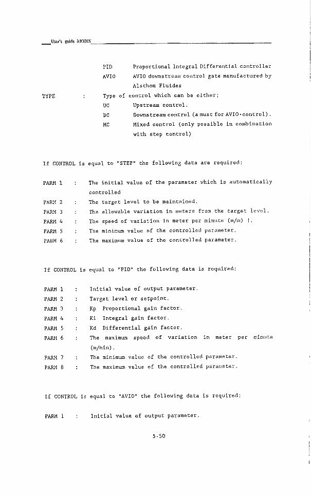
User's giife MODIS_
TYPE
PID Proportional I n t e g r a l D i f f e r e n t i a l c o n t r o l l e r
AVIO AVIO dovmstream c o n t r o l gate manufactured by
Alsthom F l u i d e s
Type of c o n t r o l which can be e i t h e r ;
UC Upstream c o n t r o l .
DC Dovmstream c o n t r o l (a must f o r A V I O - c o n t r o l ) .
MC Mixed c o n t r o l ( o n l y p o s s i b l e i n combination
w i t h step c o n t r o l )
I f CONTROL i s equal to "STEP" the f o l l o w i n g data a re r e q u i r e d :
PARM 1
PARM 2
PARM 3
PARM 4
PARM 5
PARM 6
The i n i t i a l v a l u e of the parameter which i s a u t o m a t i c a l l y
c o n t r o l l e d
The t a r g e t l e v e l to be maintained.
The allowable v a r i a t i o n i n meters from the t a r g e t l e v e l .
The speed of v a r i a t i o n i n meter per minute (m/m) !.
The minimum va l u e of the c o n t r o l l e d parameter.
The maximum value of the c o n t r o l l e d parameter.
I f CONTROL i s equal to "PID" the f o l l o w i n g data i s r e q u i r e d ;
PARM 1
PARM 2
PARM 3
PARM 4
PARM 5
PARM 6
PARM 7
PARM 8
I n i t i a l v a l u e of output parameter.
Target l e v e l or s e t p o i n t .
Kp P r o p o r t i o n a l g a i n f a c t o r .
K i I n t e g r a l gain f a c t o r .
Kd D i f f e r e n t i a l g a i n f a c t o r .
The maximum speed of v a r i a t i o n i n meter per minute
(m/min).
The minimum va l u e of the c o n t r o l l e d parameter.
The maximum va l u e of the c o n t r o l l e d parameter.
I f CONTROL i s equal to "AVIO" the f o l l o w i n g data i s r e q u i r e d :
PARM 1 I n i t i a l v a l u e of output parameter.
5-50
Nïodel defiuiüoQ
Target: l e v e l or setpoint:.
X r a d i a l , r a d i u s of the gate i n cm
Decrement of the c o n t r o l l e r i n cm
damp, c r o s s - s e c t i o n a l a r e a of f l o a t e r opening i n cm2
The minimum v a l u e of the c o n t r o l l e d parameter.
The maximum va l u e of the c o n t r o l l e d parameter.
I f TYPE i s equal to "MC" (only p o s s i b l e i n combination with step-
c o n t r o l l e r ) the f o l l o w i n g data i s r e q u i r e d :
PARM 1
PARM 2
PARM 3
PARM 4
PARM 5
PARM 6
PARM 7
PARM 8
The i n i t i a l v alue of the parameter which i s a u t o m a t i c a l l y
c o n t r o l l e d
The lower upstream t a r g e t l e v e l .
The upper upstream t a r g e t l e v e l .
The downstream t a r g e t l e v e l .
The a l l o w a b l e v a r i a t i o n i n meters from the downstream
t a r g e t l e v e l .
The speed of v a r i a t i o n i n meter per minute (ra/min) !.
The minimum value of the c o n t r o l l e d parameter.
The maximum va l u e of the c o n t r o l l e d parameter.
A l l parameters (except the I n i t i a l v alue of a STEP c o n t r o l l e r ) , can be
given as a constant v a l u e or as a f u n c t i o n of other v a r i a b l e s using the
stand a r d r e f e r e n c e convention a l r e a d y d i s c u s s e d i n paragraph 5.5.1 (Table
5.6.1). The r e f e r e n c e convention c o n s i s t s of four p a r t s .
1) A one c h a r a c t e r code f o r the type of the independent v a r i a b l e . H, T,
U, e t c e t e r a . (Table 5.6.1).
2) A one c h a r a c t e r code f o r the f u n c t i o n type. The f o l l o w i n g f u n c t i o n
types are a v a i l a b l e : T - Tabulated form
F - F o r t r a n d e f i n e d f u n c t i o n
3) A f t e r the two c h a r a c t e r codes s e l e c t e d from the l i s t , the symbol "$"
must be given.
4) F i n a l l y the name of the f u n c t i o n must be given. The name i s l i m i t e d
up to 7 c h a r a c t e r s .
5-51
User's guide MODIS_
T A B L E 5.6.1 Function references for automatic control parameters
PART 1 : Code D e s c r i p t i o n
T - Time
H - Water l e v e l
Z - C r e s t l e v e l
A - Cross s e c t i o n a l Area of opening
U - Upstream head over the s t r u c t u r e
D - D e v i a t i o n from s e t - p o i n t ( a l l o w s f o r m u l t i p l e speed)
0 - Opening height of the gate
Y - R a t i o gate opening height/upstream head
PART 2 : Code D e s c r i p t i o n
T - Tabulated form
F - F o r t r a n f u n c t i o n
A - Automatic c o n t r o l
PART 3 : $ ( d o l l a r s i g n )
PART 4 : Users d e f i n e d name, maximum 7 c h a r a c t e r s
Remark : head i s d e f i n e d as water l e v e l minus c r e s t l e v e l of s i l l .
I f a l l c o n t r o l data have been s p e c i f i e d t h i s input block i s c l o s e d by a
l i n e w i t h the symbol "-" i n the f i r s t column. The input segment i s c l o s e d
by a l i n e c o n t a i n i n g "*END" i n the f i r s t four columns.
An example of the input segment *AULC i s given i n F i g . 5.6.1
5-52

Modd defixiitioo
*AULC AUTOMATIC LOCAL CONTROL
+
+NAME CONTROL TYPE INI VAL TARG L DEAD BAND SPEED MIN MAX
C0NTR2 STEP UC 1.10 10.30 0.02 0.01 0.00 1.50
+
+NAME CONTROL TYPE i n i v a l TARGET L Kp K i Kd SPEED MIN L̂AX
CONTRl PID UC 1.20 10.30 3.5 0.5 1.5 0.10 0.0 1.50
+NAME CONTR TYPE INI TARG X (cm) deer (cm) damp (cm2) rain max
CNTRl AVIO DC 0.28 10.70 28. 1.4 15. 0.0 0.25
*END
Fig. 5.6.1 Example of Input segment *AULC (automatic local control)
5-53

User's guide MODIS
5.6.3 Automatic regional control
Automatic r e g i o n a l c o n t r o l i m p l i e s t h a t two (or thre e ) water l e v e l s
l o c a t e d along the c a n a l , e i t h e r upstream or downstream of the s t r u c t u r e ,
are used to c o n t r o l a s t r u c t u r e . Under the heading:
*AURC - automatic r e g i o n a l c o n t r o l
+NAME CONTROL TYPE PARM 1 PARM 2 PARM 3 PARM 4 PARM 7
The f o l l o w i n g data have to be given:
NAME : Name of the c o n t r o l l e r (maximum 10 c h a r a c t e r s ) .
GRDl : Name of the f i r s t g r i d p o i n t .
GRD2 : Name of the second g r i d p o i n t .
GRD3 : Name of the t h i r d g r i d p o i n t (Only f o r CARDD-control).
TYPE ; Type of c o n t r o l l e r which can be e i t h e r :
I f TYPE i s equal to "BIVAL" the f o l l o w i n g a d d i t i o n a l data w i l l be
r e q u i r e d :
INITVAL
PID P r o p o r t i o n a l I n t e g r a l D i f f e r e n t i a l c o n t r o l l e r
BIVAL BIVAL c o n t r o l system
I n i t i a l v a l u e of parameter which i s a u t o m a t i c a l l y
c o n t r o l l e d .
TARGETL Target l e v e l to be maintained
ALPHA val u e of alpha which determined the l o c a t i o n of the
piv o t p o i n t . X(p) - X ( g r d l ) + (1-alpha) ( X ( g r d 2 ) -
X ( g r d l ) )
QMAX
DEADB
DECR
Maximum d i s c h a r g e of the c a n a l reach a t p i v o t p o i n t
Dead band of the st e p c o n t r o l l e r . Note t h a t the
allowable v a r i a t i o n i s equal to TARGETL ± 1/2 DEADB !
Decrement of the water l e v e l from the t a r g e t l e v e l a t
the p i v o t p o i n t f o r zero d i s c h a r g e .
MIN
SPEED Speed of c o n t r o l parameter i n meter per minute m/m.
Minimum v a l u e of c o n t r o l parameter.
MAX Maximum v a l u e of c o n t r o l parameter.
5-54

Modd definidon
I f CONTROL i s equal to "PID" the f o l l o w i n g data w i l l be r e q u i r e d :
ALPHA : v a l u e of alpha which determined the l o c a t i o n of the
p i v o t p o i n t . X(p) - X ( g r d l ) + (1-alpha) { X ( g r d 2 ) -
X ( g r d l ) )
Kp : Kp P r o p o r t i o n a l gain f a c t o r .
K i : K i I n t e g r a l gain f a c t o r .
Kd : Kd D i f f e r e n t i a l gain f a c t o r .
SPEED : The maximum v a r i a t i o n i n meter per minute m/m.
MIN : The minimum v a l u e of the c o n t r o l l e d parameter.
MAX : The maximum va l u e of the c o n t r o l l e d parameter.
I f CONTROL i s equal to "CARDD" the f o l l o w i n g data, apart from the
a d d i t i o n a l g r i d p o i n t , w i l l be r e q u i r e d :
INTERVAL : The i n t e r v a l (sample p e r i o d ) between which new gate
s e t t i n g s are c a l c u l a t e d .
SPEED : The maximum v a r i a t i o n i n meter per minute (ra/ra).
MIN : The minimum v a l u e of the c o n t r o l l e d parameter.
MAX : The maximum va l u e of the c o n t r o l l e d parameter.
Furthermore, 11 c o n s t a n t s have to be s p e c i f i e d which are f i x e d f o r the
t o t a l CARDD-system. These constants are d e f i n e d i n a new input b l o c k
named *CARDD. A f t e r t h i s s t e e r - k e y , the value of the 11 parameters are
given i n sequence on one input l i n e , see example below.
*CARDD
+ C l C2 C3 C4 C5 C6 C7 C8 C9 CIO C l l
200 60 0.0015 0.01 0.15 1.60 0.03 4.50 0.075 0.005 0.5
A l l parameters ( e x c e p t the i n i t i a l v a l u e of a STEP c o n t r o l l e r ) , can be
given as a c o n s t a n t v a l u e or as a f u n c t i o n of other v a r i a b l e s u s i n g the
sta n d a r d r e f e r e n c e convention a l r e a d y d i s c u s s e d i n paragraph 5.6.1.
I f a l l c o n t r o l data have been s p e c i f i e d t h i s input b l o c k i s c l o s e d by a
l i n e w i t h the symbol "-" i n the f i r s t column.
5-55

L W s guide MODIS
An example of the input segment *AURC i s given i n F i g . 5.6.2
*AURC AUTOMATIC REGIONAL CONTROL
+NAME GRDl GRD2 CONTR INIV TARGETL ALPHA Kp K i Kd SPEED MIN MAX
+
CNTRl G12 G21 PID 0.40 111.580 0.67 -1.5 -0.1 -0.0 1. 0.0 1.30
+
+NAME GRDl GRD2 CONTR INIV TARGETL ALPHA QMAX DEADB DECR SPEED MIN MAX
CNTR2 G22 G31 BIVAL 0.4 111.580 0.67 15.0 0.04 0.0 0.05 0.0 1.30
*END OF ACSDEF
Fig. 5.6.2 Example of input segment *AURC (automatic regional control)
5-56

definidon^
.cfilobaUonWO» l e v e l s Automatic gl ot
5.6.4 ^ any " .̂ ^̂ ,„1 impli-^^ ^ s t r u c t u r e -
r e q u i r e d . ^^^xity of 6 ^
t e s t the apV^^
tob a l c o n t r o l SJ^ED , automatic global ^ ^ ^ E T
CONTROL
_ _ ^ i € i e d . ,_„.̂ tniu
XV,e f o U o v i ^ S
NAME
CONTROL
XARGEIL
Xï^tER^^^
SPEED
1'VAX
. . xo c h a r a c t e r s ) •
t̂ aroe ot v , i c V i c a n b e • c o n t r o l
L i n e a r 4" „Y,ich i - ^
W ° xue of parameter
X n i t l a l v a l u e
^ ^ ^ l e c a l c u l a t e d . . I n u t e Cm/m) •
v a r i a t i o n ' parameter.
^ ^ ' ^ " ^ : l e o f t h e — ^ ; : , V . a m e t e r .
maximum vaX ^̂ ^̂^ _^
^^rmbol
11^ • The maximum vaXu _^ ^.
- ^ ^ ^ ^ , . e . - —
t h l o c ^ i s
Tbe i n P - t named
column. - ^ -
^XocU i s o^os.^
rhe i n P - t named
c o l " " - ^ „ ,t.«l£'"'
" " " " " 0 » »
*GLGR GRD^
,GRD1
5-57

guiite
P l a c e d on '^an be . "
" De p,-„ f a c t „ °£^aer an^ j
3 . ^' « number o f
headed b
f„i, ^ a c h a r a ^ ^
Control ''^ices are
"''Server;
and a ^ ^ ' ^ ^ ^ i
" ^^^^^ - a r z a b i e
> p e r i o d an^ the i-pp ""̂
" '̂ i'-'e l e v e l ^ ' ' ^ " ^ " t )
" '"P"^ v a r i a b l e
• output /
" " - " - - e mode.
i c
5-58
Model definidoQ
The m a t r i c e s to be d e f i n e d a r e :
*PHIH - *
*GAMM - r
*CMAT - C
*KFMA - Kf
*KSMA - Ks
*WMAT - W
*HMAT - H
*KDMA - Kd ( E x t r a m a t r i x )
I f one matr i x i s not used, i t can simply be skipped. The data i n the
mat r i x e s a re j u s t f i g u r e s separated by one or more blank spaces. There
i s no l i m i t a t i o n of the number of matrix element as long as the a r r a y
dimensions ( s p e c i f i e d i n \modis\include\matrix.add) are not exceeded.
The i n p u t segment i s c l o s e d by a l i n e c o n t a i n i n g "*END" i n the f i r s t four
columns.
An example of the input segment *AURC i s given i n F i g . 5.6.4
5-59

L'ser's guide MODIS
5.7 Functions
If no functions are used, this part can be skipped. The input segment Functions consist of three input
blocks
*TTIM - tabulated functions of time
°TGFU - tabulatedgeneral function
• F D F U - fortran defmed functions
The first input block ("ITIM) is reserved for variables of which the values have been defined previously
to be a function of time. The second and third input block is for all other functions. Preferabletabulated
functions should be used, as for fortran functions, the function has to be written, compiled and linked
to the program package, which takes some more time.
5.7.1 Tabulated functions of lime
Under the heading
*TTIM - TABULATED FUNCTIONS OF TIME
Following the i d e n t i f i c a t i o n l i n e the input c o n t i n u e s w i t h a l i n e of the
form:
NAME FUNl FUN2 FUN3 FUN4 FUN5
The f i r s t name should always r e a d "NAME". The names FUNl, FUN2, e t c are
user d e f i n e d names. On one l i n e a maximum of 10 f u n c t i o n s can be given
with v a l u e s f o r the independent v a r i a b l e i n the f i r s t data column and
va l u e s f o r dependent v a r i a b l e s i n s u c c e s s i v e data columns. The input
i d e n t i f i c a t i o n l i n e s f o r f u n c t i o n s can be re p e a t e d any number of times
i n any order to add more f u n c t i o n s to the input f i l e . Obviously t h i s
freedom holds as long as no a r r a y l i m i t s f o r s t o r i n g the data are
exceeded. The f i r s t input s t r i n g (under the header "NAME") i s r e s e r v e d
fo r the f u n c t i o n v a r i a b l e time s p e c i f i e d i n e i t h e r dhms or second
n o t a t i o n .
5-60

Modd defmitioa
<n t a b l e form With on each l i n e
order.
M t h i s i n put block i s closed by a 1 data have been s p e c i f i e d t h i s mp
Xf a l l c o n t r o l data ha ^^^^^ ^^^^^^
U n e w i t h the symbol
• . block *TTIH i s given i n F i g . 5.7.1 An example of the input block
*TTIM
NAKE
+
0:00:00-.00
0-.12:00'.00
01-.00-.00-.00
01-.12-.00-.00
02:00:00:00
02 •.12-. 00; 00
03;00:00:00
03:12:00:00
04:00:00:00
TABULATED FUNCTIONS OF TIME
QUrSTREAM l i ^ Q R ^^"'^
70.
98.
175.
324.
341.
270.
212.
164.
120.
5.20
5.30
2.40
25.50
25.50
22.00
21.00
21.00
21.50
21.50
22.00
25.00
Fig. 5.7.1 o. « P « - ™ " " " " "
of
time)
5-61

Modd deimitioo
As a next input item the v a l u e s a r e g i v e n i n t a b l e form w i t h on each l i n e
the value of the independent v a r i a b l e , f o l l o w e d by the f u n c t i o n v a l u e ( s ) .
The v a l u e s of the independent v a r i a b l e have to be given i n i n c r e a s i n g
order.
I f a l l c o n t r o l data have been s p e c i f i e d t h i s input b l o c k i s c l o s e d by a
l i n e with the symbol "-" i n the f i r s t column.
An example of the input b l o c k *TTIM i s given i n F i g . 5.7.1
*TTIM - TABULATED FUNCTIONS OF TIME
NAME QUPSTREAM LARQR BIDIV
+
0:00:00:00 70. 5.20 25. 50
0:12:00:00 98. 5.30 25, ,50
01:00:00:00 175. 2.40 22, ,00
01:12:00:00 324. _ 21 ,00
02:00:00:00 341. - 21, .00
02:12:00:00 270. - 21 .50
03:00:00:00 212. - 21 .50
03:12:00:00 164. - 22 .00
04:00:00:00 120. 25 .00
Fig. 5.7.1 Example of input block *TTFU (tabulated functions of
time)
5-61

Modtl definidou
An example of the input block *TGFU i s given i n F i g . 5.7.2
*TGFU- GENERAL TABULATED FUNCTIONS
+
NAME CELL2 AREARES
+ H AREA AREA
8.00 0.0E7 5.E7
10.00
12.00
14.00 - 1.E8
Fig. 5.7.2 Example of input block ^TGFV (Tabulated genera
functions)
5-63

L W s guide MODIS_
5.7.3 Fortran defined functions
I n s t e a d of a tab u l a t e d f u n c t i o n , mathematical f u n c t i o n s can sometimes be
used, f o r example to s i m u l a t e the water l e v e l i n a t i d a l r i v e r with a
s i n u s o i d a l water l e v e l f l u c t u a t i o n . I n order to do so, the u s e r can w r i t e
h i s own fu n c t i o n as a F o r t r a n f u n c t i o n and compile and l i n k t h i s
f u n c t i o n .
Under the header
*FDFU - F o r t r a n d e f i n e d f u n c t i o n s
+
+ NAME
The name of the f u n c t i o n i s s p e c i f i e d .
Where
NAME : name of f o r t r a n s t r u c t u r e (max 10 c h a r a c t e r s )
I f a l l names have been s p e c i f i e d t h i s input block i s c l o s e d by a l i n e
w ith the symbol "-" i n the f i r s t column.
The user now has to w r i t e a subprogram i n F o r t r a n f o r the f u n c t i o n . T h i s
i s done by reading the f i l e MODCOMXF.FOR i n an e d i t o r and changing the
subprogram FFUN. The new f u n c t i o n r o u t i n e e.g SIN i s w r i t t e n i n t h i s same
f i l e . Then the program i s saved, compiled and l i n k e d to modcom.exe. (See
a l s o paragraph 5.5.9, F o r t r a n s t r u c t u r e s ) .
5-64
Model defiiudoa
5 . 8 Initial state
I n t r o d u c t i o n
The l a s t input segment of the input f i l e f o r subsystem MODRES i s che
i n i t i a l s t a t e . For the numerical i n t e g r a t i o n of the equations d e s c r i b i n g
the unsteady flow i n an open c a n a l system, an i n i t i a l s t a t e i s needed i n
every g r i d p o i n t . However the u s e r does not need to give i n i t i a l data i n
each g r i d p o i n t .
For each branch i n i t i a l data (water l e v e l and d i s c h a r g e ) have to be given
a t l e a s t at the end g r i d p o i n t s . At g r i d p o i n t s between the given p o i n t s
the system w i l l generate v a l u e s by l i n e a r i n t e r p o l a t i o n or c a l c u l a t e them
from a given f u n c t i o n of x. The system w i l l f i r s t s e t v a l u e s a t the
p o i n t s s p e c i f i e d by the user and then f i l l the gaps by l i n e a r i n t e r
p o l a t i o n or c a l c u l a t i o n from the s p e c i f i e d f u n c t i o n s . T h i s i m p l i e s tha t
input i s not bound to a c e r t a i n sequence. However, i t i s a d v i s e d Co group
the input per branch and separate Chese groups by blank commenC l i n e s .
I f Che i n i c i a l sCate s p e c i f i e d by the u s e r i s very d i f f e r e n t from a
r e a l i s t i c i n i t i a l s t a t e , the program might f a c e so c a l l e d n o n - l i n e a r
i n s t a b i l i t y problems. These i n s t a b i l i t i e s can be avoided by g i v i n g a more
a c c u r a t e d e f i n i t i o n of the i n i t i a l s t a t e . A simple i n i t i a l s t a t e i s to
de f i n e h o r i z o n t a l water l e v e l s w i t h zero d i s c h a r g e s .
Input
The input i d e n t i f i c a t i o n l i n e f o r t h i s item reads as;
*INST DEFINITION OF INITIAL STATE
+ BRANCH GRID POINT DEFINITION OF H DEFINITION OF Q
+ TYPE VALUE/REFERENCE TYPE VALUE/REFERENCE
Data are given i n the form of data columns. Each input l i n e s p e c i f i e s the
i n i t i a l s t a t e a t a u s e r - d e f i n e d g r i d p o i n t .
5-65
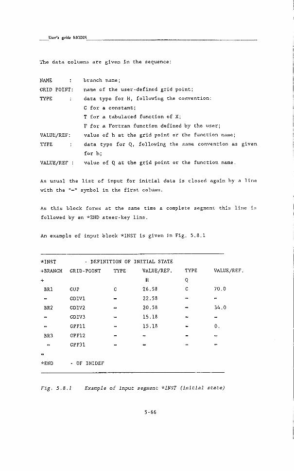
User's guide MOOIS
The data columns are gi v e n i n the sequence:
NAME : branch name;
GRID POINT; name of the u s e r - d e f i n e d g r i d p o i n t ;
TYPE : data type f o r H, f o l l o w i n g the convention:
C f o r a co n s t a n t ;
T f o r a t a b u l a t e d f u n c t i o n of X;
F f o r a F o r t r a n f u n c t i o n defined by the user;
VALUE/REF: v a l u e o f h a t the g r i d point or the f u n c t i o n name;
TYPE : data type f o r Q, f o l l o w i n g the same convention as gi v e n
f o r h;
VALUE/REF : v a l u e of Q a t the g r i d point or the f u n c t i o n name.
As u s u a l the l i s t of input f o r i n i t i a l data i s c l o s e d again by a l i n e
w i t h the "-" symbol i n the f i r s t column.
As t h i s b l o c k forms a t the same time a complete segment t h i s l i n e i s
fol l o w e d by an *END s t e e r - k e y l i n e .
An example of input b l o c k *INST i s given i n F i g . 5.8.1
*INST
+BRANCH
+
BRI
BR2
BR3
DEFINITION OF INITIA L STATE
GRID-POINT
GUP
GDIVl
GDIV2
GDIV3
G P F l l
GPF12
GPF31
TYPE VALUE/REF.
H
26.58
22.58
20.58
15.18
15.18
TYPE
Q
C
VALUE/REF.
70.0
34.0
*END - OF INIDEF
Fig. 5.8.1 Example of Input segment *INST (initial state)
5-66
6 Model computation
6.1 Introduction
The r e a l computations are performed by the computational subsystem c a l l e d
MODCOM (MODel COMputation). This system reads the model d e f i n i t i o n , which
has been processed by MODDEF, from the model data base, and s t a r t s the
simu l a t i o n . The data t o c o n t r o l the simu l a t i o n process have t o be
supplied on an input f i l e named COMIN.DAT. This input f i l e consists of
one segment which i s made up of nine input blocks. These input blocks
are:
*IDEN - run i d e n t i f i c a t i o n ;
*SWIT - run switches;
*PARM - numerical and general physical parameters;
*TIME - time c o n t r o l parameters;
•RSST - system state r e s u l t data f i l e ;
*RTIF - r e s u l t time f u n c t i o n f i l e ;
«ROUT - route d e f i n i t i o n s through net
«BASF - r e s u l t base functions;
*RPLF - r e s u l t place functions.
Each input block i s described i n d e t a i l i n the f o l l o w i n g of t h i s chapter.
6-1

User's guide MODIS_
6 .2 R u n control parameters
6.2.1 Run identirication
The f i r s t input block of the input f i l e f o r the model computation i s used
t o i d e n t i f y the input and output f i l e s . Normally the user can leave t h i s
input block unchanged.
The i d e n t i f i c a t i o n block s t a r t s w i t h the steer-key l i n e :
*IDEH - RUN IDENTIFICATION
+
+ DATASET (FILENAMES)
+
< >
INPUT f i l e name \
ECHO f i l e name )- •consistent w i t h
OUTPUT f i l e name /
MODDB f i l e name \
SST FILE f i l e name )- •defined here
PLF FILE f i l e name )
RTF FILE f i l e name /
The codes i n c a p i t a l s have t o be copied e x a c t l y .
The f i l e names are given by the user and should not s t a r t before column
20. Normally standard names are used (see Fig. 6.2.1).
At the end of t h i s input block a l i n e i s given w i t h the character '-' i n
the f i r s t column.
6-2
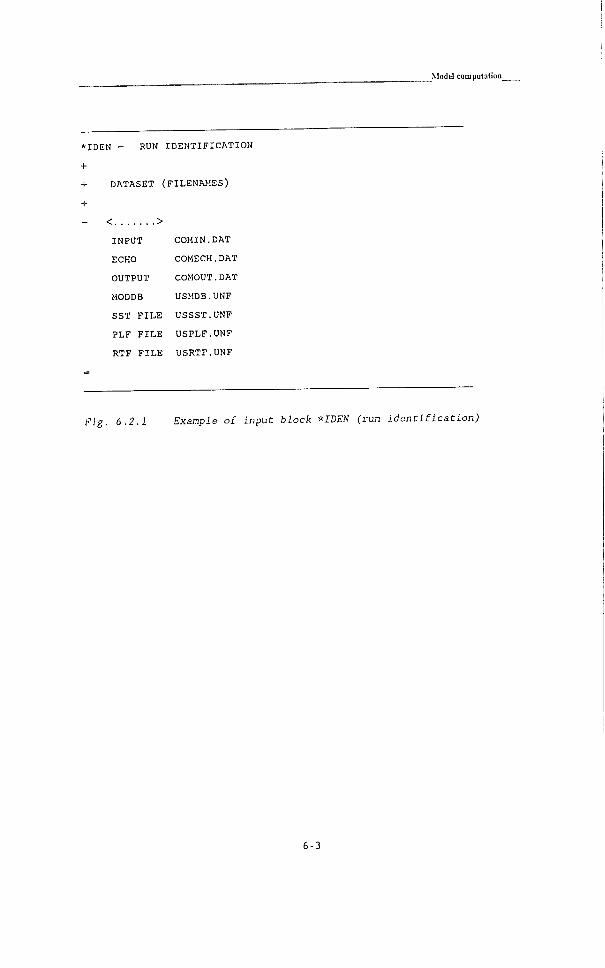
Model computation.
* I D E N
+
+
+
RUN I D E N T I F I C A T I O N
D A T A S E T ( F I L E N A M E S )
< >
I N P U T
ECHO
OUTPUT
MODDB
COMIN.DAT
COMECH.DAT
COMOUT.DAT
USMDB.UNF
S S T F I L E U S S S T . U N F
P L F F I L E U S P L F . U N F
R T F F I L E U S R T F . U N F
Fig. 6.2.1 Example of input block *IDEN (run Identification)
6-3

User's guide MODIS
6.2.2 Switches
The switch parameters a c t i v a t e or deactivate data t r a n s f e r , c r e a t i o n of
new f i l e s , debug f a c i l i t i e s and the p r i n t i n g of t h e i r r e s u l t i n g output.
These switches have t o be given i n a s p e c i f i c sequence t o i n d i c a t e the
names (these appear i n a l i s t on a comment l i n e ) . On the input l i n e below
the comment l i n e , the f o l l o w i n g characters can be given:
Y t o a c t i v a t e the switch (abbreviation of YES);
N t o deactivate the switch (abbreviation of KO).
t t o set the d e f a u l t
On each l i n e 7 switches are read. Some p o s i t i o n s have no meaning y e t , as
indicated by the heading 'FREE'. Here the d e f a u l t character 't' has t o
be given.
The switches w i t h t h e i r meaning are given below i n the sequence i n which
they appear i n the input.
l i n e 1
TEST some general t e s t output
TESTC t e s t output computational algorithm
TESTS t e s t output s t r u c t u r e s
TESTO t o switch out the computational r o u t i n e COMSYS and
ac t i v a t e dummy computational r o u t i n e DUMCOM
DEBUG log f i l e f o r r e s u l t data base actions
LOCONTR w r i t i n g the computed l o c a l c o n t r o l output signals t o
output f i l e (comout.dat).
RECONTR w r i t i n g the computed regio n a l c o n t r o l output signals t o
output f i l e (comout.dat), but only i f LOCONTR - N.
Remark on LOCONTR and RECONTR:
Only one of the switches LOCONTR or RECONTR should be 'Y', and the other
switch should be 'N'.
6-4
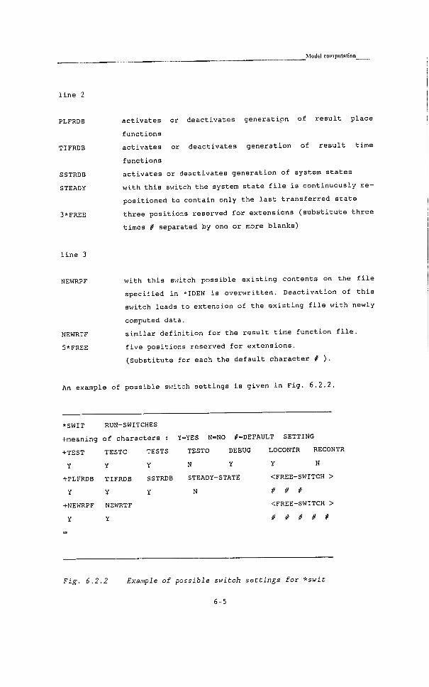
Model computatioa^
l i n e 2
PLFRDB
TIFRDB
SSTRDB
STEADY
3*FREE
activates or deactivates generation of r e s u l t place
functions
a c t i v a t e s or deactivates generation of r e s u l t time
functions
activates or deactivates generation of system states
w i t h t h i s switch the system st a t e f i l e i s continuously r e
positioned to contain only the l a s t t r a n s f e r r e d s t a t e
three positions reserved f o r extensions ( s u b s t i t u t e three
times # separated by ona or more blanks)
l i n e 3
NEWRPF
NEWRTF
5*FREE
w i t h t h i s switch possible e x i s t i n g contents on the f i l e
s p e c i f i e d i n *IDEN i s o v e r w r i t t e n . Deactivation of t h i s
switch leads to extension of the e x i s t i n g f i l e w i t h newly
computed data.
s i m i l a r d e f i n i t i o n f o r the r e s u l t time f u n c t i o n f i l e ,
f i v e positions reserved f o r extensions.
(Substitute for each the d e f a u l t character # ) .
An example of possible switch s e t t i n g s i s given i n Fig. 6.2.2.
*SWIT RUN-SWITCHES
+raeaning o f characters : Y-YES N-NO ^-DEFAULT SETTING
+TEST TESTC TESTS
Y Y Y
+PLFRDB TIFRDB SSTRDB
Y Y Y
+NEWRPF NEWRTF
Y Y
TESTO DEBUG
N Y
STEADY-STATE
N
LOCONTR RECONTR
Y N
<FREE-SWITCH >
i f f
<FREE-SWITCH >
# # # # #
Fig. 6.2.2 Example of possible switch settings for *swit
6-5
_Uscr's guide MODIS_
6.3 Computational parameters
The computational parameters are given i n the input block *PARM
i d e n t i f i e d by:
"FARM - NUMERICAL AND PHYSICAL PARAMETERS
+ PSI THETA ITERM G
+ EPSOFL EPSUFL EPSHFL EPSDH
Were:
PSI
THETA
ITERM
i s the weighting c o e f f i c i e n t f o r the d i s c r e t i z a t i o n s i n x.
Usually a value of 0.5 i s given;
i s the weighting c o e f f i c i e n t f o r the d i s c r e t i z a t i o n s i n
time. For accurate computations a fac t o r of 0.55 i s given.
For steady state computations i t i s advantageous t o take
a f a c t o r close t o 1, i n order t o damp undesired
osculations and to converge q u i c k l y t o the steady s t a t e ,
i s the number of i t e r a t i o n steps w i t h i n one time step. As
a r u l e i t does not make sense t o take a value d i f f e r e n t
from 2.
i s the acceleration due to g r a v i t y . A value of 9.82
u s u a l l y i s accurate enough.
The second l i n e of computational parameters concern some numerical t e s t
values used during the evaluation of s t r u c t u r e functions. (When t h i s
second i n p u t l i n e i s skipped the d e f a u l t values given between brackets
are used).
EPSOFL
EPSUFL
EPSHFL
EPSDH
Test value f o r dh whether l i n e a r i z a t i o n i s required f o r
overflow s t r u c t u r e s . Usual value i s 0.01
Test value for l i n e a r i z a t i o n f o r underflow s t r u c t u r e s .
Usual value i s 0.01
Test value f o r l i n e a r i z a t i o n f o r head loss s t r u c t u r e s .
Usual value i s 0.01
Increment value f o r water l e v e l used during numerical
d i f f e r e n t i a t i o n of s t r u c t u r e s . Usual value i s 0.01
6-6

Model computation
The input block i s closed by a l i n e containing the symbol "-" i n the
f i r s t column. An example of input block *PARM i s given i n Fig. 6.3.1
*PARM - NUMERICAL AND PHYSICAL PARAMETERS
+
+ PSI THETA ITERM G
0.5 0.55 2 9.82
+ EPSOFL EPSUFL EPSHFL EPSDH
0.01 0.01 0.01 0.01
Fig. 6.3.1 Example of input block *PAR}i (compucaclonal parameCers)
6-7
User's guide MODIS
6.4 Time control parameters
I n the input block f o r time c o n t r o l parameters values have t o be given
t o c o n t r o l the s t a r t and the end time f o r the computations. Besides the
time step and what system s t a t e i s used t o ( r e ) s t a r t the system f i l e have
t o be s p e c i f i e d . Data are given under the header:
*TIME - TIME CONTROL PARAMETERS
+
+ BEGIN-TIME END-TIME TIME-STEP SST-TIME
Where:
BEGIN TIME i s the s t a r t i n g time of the si m u l a t i o n . Like many other
time values time i s given as e i t h e r i n seconds or a time
s t r i n g i n dhms - no t a t i o n i . e . D:H:M:S, w i t h :
D the number of days (1,2 or 3 d i g i t s ) ;
H the number of hours (2 d i g i t s ) ;
M the number of minutes (2 d i g i t s ) ;
S the number of seconds (2 d i g i t s ) .
END TIME i s the end time of the simu l a t i o n period given i n time
s t r i n g format as described above or i n seconds. Simulation
i s terminated as soon as t h i s moment i s reached.
TIME STEP s p e c i f i e s the time step t o be used by the system.
The f o l l o w i n g options are a v a i l a b l e :
- a constant time step given as a time s t r i n g i n dhms
n o t a t i o n ;
the time step i n seconds (upto two d i g i t s behind the
p o i n t ) .
- a time step given as a tab u l a t e d f u n c t i o n of time. The
s p e c i f i c a t i o n reads T$<name>. The t a b l e i s supposed t o
be s p e c i f i e d i n input segment FUNCTION of subsystem
MODDEF.
- a time step given by a Fortran defined f u n c t i o n of
time. I n t h i s case the s p e c i f i c a t i o n reads FS<name>.
The f u n c t i o n <name> has t o be c a l l e d and defined i n
the i n t e r f a c e r o u t i n e FFUN.
6-8
Model compuLaüoo
SST-TIME specifies a s t r i n g informing the system how to read the
i n i t i a l state from the system s t a t e f i l e . Possible options
are:
INIDEF the system w i l l read the system state from the
SST-flie, which was defined i n INIDEF (i n p u t
segment of MODDEF);
PERM the system w i l l t r y t o read an i n i t i a l s t a t e f o r
the SST f i l e which was previously w r i t t e n by
system MODCOM during a steady state run w i t h the
steady s t a t e switch on Y(es). Beware t h a t the
system generated steady s t a t e w i l l be destroyed
i f MODDEF i s run w i t h the INIDEF-switch on Y. So
to avoid t h i s o v e r w r i t t i n g of the system
generated steady s t a t e , the INIDEF-switch should
be set on N, a f t e r a steady state has been made.
BEGIN the system w i l l read the system state from the
SST-flie w i t h the l a s t time l e v e l <- BEGIN-TIME.
Some a d d i t i o n a l explanation has t o be given on the time step d e f i n i t i o n
i n general. During input processing the system generates moments i n time
where during the simulation the process i s forced t o a r r i v e at a
computational time l e v e l . This i s used f o r instance, t o generate r e s u l t
place functions at a s p e c i f i c moment i n time. Due t o t h i s algorithm the
time step r e a l l y used can be somewhat smaller then the one s p e c i f i e d by
the user. The time step a c t u a l l y used i s shown i n the system log on the
echo f i l e .
An example of input block *TIME i s depicted i n Fig. 6.4.1
*TIME TIME CONTROL PARAMETERS
+BEGIN-TIME END-TIME TIME-STEP SST-USAGE
00:00:00:00 01:03:00:00 T5DELTA-T INIDEF
Fig. 6.4.1 Example of input block *TIHE (run time specification)
6-9
User's guide MODIS_
6.5 Output to the system state file
Time i n t e r v a l s have t o be s p e c i f i e d i n order t o w r i t e r e s u l t s of the
computations t o the System State Result Data f i l e ( S S T - f l i e ) . The system
state r e s u l t data f i l e contains a complete d e s c r i p t i o n s p e c i f i e d i n h and
Q of the system at a c e r t a i n moment i n time. This system s t a t e can be
used l a t e r t o r e s t a r t a computation. The parameters t o c o n t r o l the system
state f i l e actions have t o be given i n the input block headed by the
i d e n t i f i c a t i o n l i n e :
*RSST SYSTEM STATE RESULT DATA FILE
+
+ BEGIN END INTERVAL
Where
BEGIN a time value a f t e r which during the simulation i t i s
checked f o r every time step whether the system has t o be
stored or not. Possible s p e c i f i c a t i o n s are:
B Checking s t a r t s immediately at the beginning of
the simulation. This i s also the d e f a u l t b u i l t - i n
value;
<time> a time s t r i n g i n dhms n o t a t i o n , or i n seconds.
END a time value a f t e r which checking can be stopped and no
data i s stored i n the f i l e . Possible s p e c i f i c a t i o n s are:
E Checking continues u n t i l the end of the
simulation. This i s also the de f a u l t b u i l t - i n
value;
<time> a time s t r i n g i n dhms n o t a t i o n or i n seconds.
INTERVAL For t h i s time i n t e r v a l the f o l l o w i n g options are defined:
N The corresponding f i l e f a c i l i t y i s not used. I n
f a c t i t i n a c t i v a t e s the input block;
<no.>* a f i l e a c t ion i s performed w i t h an i n t e r v a l of
<no.> time steps (e.g. 1 0 * ) ;
<tirae> a time s t r i n g i n dhms-notation, g i v i n g a constant
i n t e r v a l . I t i s also possible t o specify t h i s as
CS<time> time i s given i n seconds;
6-10
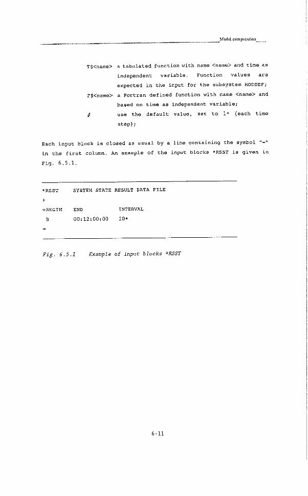
Nfodel computatioa_
TS<name> a tabulated f u n c t i o n w i t h name <name> and time as
independent v a r i a b l e . Function values are
expected i n the input f o r the subsystem MODDEF;
F$<name> a Fortran defined function w i t h name <name> and
based on time as independent v a r i a b l e ;
# use the d e f a u l t value, set t o 1* (each time
step);
Each input block i s closed as usual by a l i n e containing the symbol "="
i n the f i r s t column. An example of the input blocks *RSST i a given i n
Fig. 6.5.1.
*RSST SYSTEM STATE RESULT DATA FILE
+
+BEGIN END INTERVAL
B 00:12:00:00 20*
Fig. 6.5.1 Example of input blocks *RSST
6-11

User's guide MODIS
6.6 Output as a function of time
I n t h i s input block i t i s defined how c e r t a i n flow and geometrical
va r i a b l e s computed by the model (normally h and Q) are w r i t t e n t o a f i l e
as a f u n c t i o n of time at selected user-defined g r i d - p o i n t s .
The input block i s headed by :
*RTIF - SPECIFICATION RESULT TIME FUNCTION FILE
+ BEGIN END INTERVAL
+ TITLE GRID-POINT VAR-SPEC FUNCTION-TEXT
Where
BEGIN a time value a f t e r which during the sim u l a t i o n i t i s
checked f o r every time step whether data has t o be stored
or not. Possible s p e c i f i c a t i o n s are:
B Checking s t a r t s immediately at the beginning of
the s i m u l a t i o n . This i s also the d e f a u l t b u i l t - i n
value;
<time> a time s t r i n g i n dhms n o t a t i o n , or i n seconds.
END a time value a f t e r which checking can be stopped and no
data i s stored on the f i l e . Possible s p e c i f i c a t i o n s are:
E Checking continues u n t i l the end of the
simulation. This i s also the d e f a u l t b u i l t - i n
value;
<time> a time s t r i n g i n dhms n o t a t i o n , or i n seconds.
INTERVAL For t h i s time i n t e r v a l the f o l l o w i n g options are defined:
N The corresponding f i l e f a c i l i t y i s not used. I n
fa c t i t i n a c t i v a t e s the input block;
<no.>* a f i l e a c t i o n i s performed w i t h an i n t e r v a l of
<no.> time steps (e.g. 1 0 * ) ;
<time> a time s t r i n g i n dhms-notation, g i v i n g a constant
i n t e r v a l . I t i s also possible t o specify t h i s as
C$<time>: time i n seconds;
T$<name>: a tab u l a t e d f u n c t i o n w i t h name <name> and
time as independent v a r i a b l e . Function
6-12
Nlodd computiition^
values are expected i n the input f o r the
subsystem MODDEF;
F$<name>: a Fortran defined f u n c t i o n w i t h name <name>
and based on time as independent v a r i a b l e ;
# : use the d e f a u l t value, set t o 1* (- each
time s t e p ) ;
The r e s t of a l l «RTIF date l i n e s contain data items which define one
r e s u l t f u n c t i o n per l i n e . The s p e c i f i c a t i o n of functions i s given on
successive input l i n e s where the f o l l o w i n g input i s expected:
TITLE a f u n c t i o n t i t l e of maximum 10 characters. This f u n c t i o n
t i t l e w i l l be used l a t e r f o r a l l output presentations.
GRID POINT the name of the user-defined g r i d p o i n t where the r e s u l t
f u n c t i o n should be r e t r i e v e d .
VAR-SPEC a s p e c i f i c a t i o n of the v a r i a b l e according t o the syntax
described on the next page. The most common d e f i n i t i o n s
are HN and QN which r e t r i e v e the water l e v e l and discharge
r e s p e c t i v e l y at the end of the time step.
FUNCT.TEXT a free t e x t of maximum 40 characters. This can be used t o
give a b r i e f d e s c r i p t i o n of the f u n c t i o n . The t e x t w i l l be
reproduced i n the f u n c t i o n summary l a t e r on i n the output.
The input block i s closed by a l i n e containing the symbol "-" i n the
f i r s t column.
Variable specification
The r e s u l t s which the user wants produced on output i n the form of time
or place functions can be of very d i f f e r e n t nature. Therefore, the option
has been b u i l t - i n t o address many variables through a name s t r i n g given
i n the input. Standard s t r i n g s are:
HO water l e v e l at the beginning of the a c t u a l time step;
HN water l e v e l at the end of the ac t u a l time step;
HM the average of HO and H*; w i t h H» the water l e v e l computed
i n the one but l a s t i t e r a t i o n step;
QO, QN, QM s i m i l a r d e f i n i t i o n s f o r the discharge;
6-13

User's guide iMODIS_
A the wetted area of the cross-section
BF the flow width of the cross-section;
BS the storage width;
ESQ the Boussinesq value used;
DM the water depth
Z the bottom l e v e l
RA the h y d r a u l i c radius;
RC the resistance c o e f f i c i e n t ;
FRICM the t o t a l r esistance;
FROUDS the r e s u l t i n g Froude number.
A l l the water l e v e l dependent c o e f f i c i e n t s have been computed j u s t before
the l a s t i t e r a t i o n step, based on HM. Besides the standard r e s u l t values,
i t i s also possible t o compute any r e s u l t values by s p e c i f i c a t i o n through
the general f u n c t i o n system. As independent va r i a b l e used i n the f u n c t i o n
c a l l the g r i d p o i n t number j i s used. The options are:
TS<name> r e f e r r i n g t o a tabulated f u n c t i o n <narae>.
F$<name> r e f e r r i n g t o a Fortran defined f u n c t i o n <name>.
The l a s t option can be q u i t e u s e f u l i n special cases.
Note
A f u n c t i o n named TIME containi n g the time base i s generated a u t o m a t i c a l l y
when r e s u l t time functions are transformed i n t o GRF format by subsystem
RDBUTL.
6-14

Model computatioa^
An example of the input block *RTIF i s given i n Fig. 6.6.1
* R T I F CONTROL P A R A M ETERS FOR R E S U L T - T I M E F U N C T I O N F I L E
+
END I N T E R V A L
E t
+ B E G I N
B
+CODE
H-Gll
H - G 1 2
H - G 2 1
H - G 2 2
H-G31
H-G32
G R I D P O I N T F U N . S P E C F U N C T I O N T E X T (40 C H A R A C T E R S )
G i l HN head of the canal
G l 2 HN
G 2 1 HN
G 2 2 HN
G31 HN
G32 HN
Fig. 6.6.1 Example of inpuC block *RIIF (result time function file)
6-15

User's guide MODIS
6.7 Output as a function of place
Instead of output r e s u l t s as a f u n c t i o n of time, i t i s also p o s s i b l e t o
define output as a fu n c t i o n of place. I f t h i s i s not desired, t h i s
paragraph can be skipped. (Remember t o close the input segment w i t h *END)
I f output as a func t i o n of place i s desired three input blocks have t o
be used i n sequence.
At f i r s t i t i s needed t o define so c a l l e d "routes". A route i s a
path defined by a sequence of nodes along which output can be
produced.
- Thereafter "base r e s u l t " f unctions need t o be sp e c i f i e d which d e f i n e
an axis along a route, e.g. x-coordinated, names of g r i d p o i n t s .
F i n a l l y the variables which are given along the routes as a f u n c t i o n
of the specified axis, are defined.
6 .7 .1 De f i n i t i on of routes
Under the heading:
*ROUT
+
+ ROUTE NODES
+
The f o l l o w i n g data are required:
ROUTE user defined name of a route, f o l l o w i n g the standard name
convention.
NODES name of node, already defined i n the input f i l e of the
model d e f i n i t i o n (see previous chapter)
The input block i s closed by a l i n e containing the symbol "-" i n the
f i r s t column. An example of input block *ROUT i s depicted i n Fig. 6 . 7 . 1 .
6 - 1 6
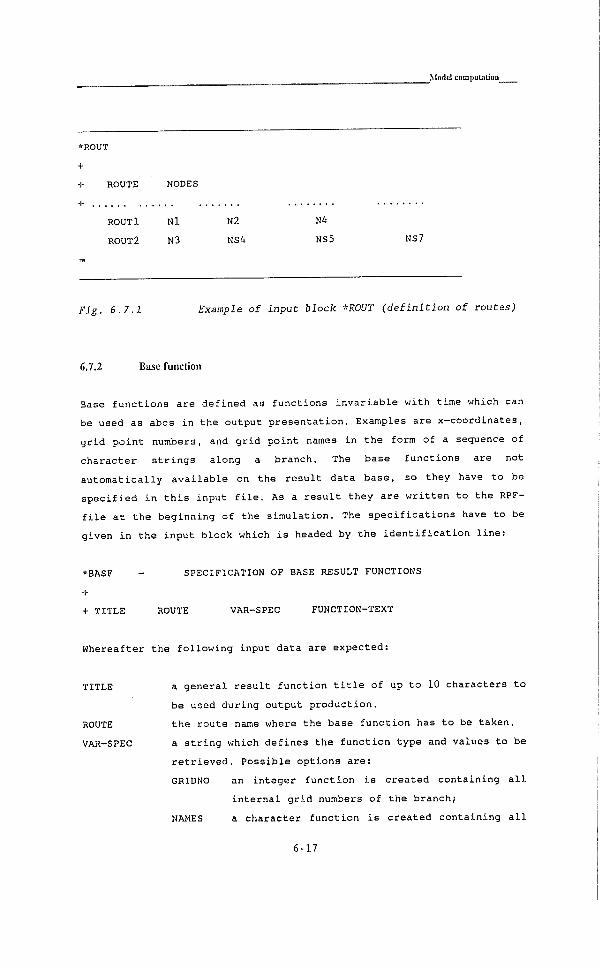
Modd computation
*ROUT
+
+ ROUTE
+
ROUTl
ROUT 2
NODES
Nl
N3
N2
NS4
N4
NS5 NS7
Fig. 6.7.1 Example of input block *ROUT (definition of routes)
6.7.2 Base f u n c t i o n
Base fun c t i o n s are defined as functions i n v a r i a b l e w i t h time which can
be used as abcs i n the output presentation. Examples are x-coordinates,
g r i d p o i n t numbers, and g r i d p o int names i n the form of a sequence of
character s t r i n g s along a branch. The base functions are not
automa t i c a l l y a v a i l a b l e on the r e s u l t data base, so they have t o be
sp e c i f i e d i n t h i s input f i l e . As a r e s u l t they are w r i t t e n t o the RPF-
f i l e a t the beginning of the simulation. The s p e c i f i c a t i o n s have t o be
given i n the input block which i s headed by the i d e n t i f i c a t i o n l i n e :
«BASF
+
+ TITLE
SPECIFICATION OF BASE RESULT FUNCTIONS
ROUTE VAR-SPEC FUNCTION-TEXT
Whereafter the f o l l o w i n g input data are expected:
TITLE
ROUTE
VAR-SPEC
a general r e s u l t f u n c t i o n t i t l e of up t o 10 characters t o
be used during output production.
the route name where the base f u n c t i o n has t o be taken,
a s t r i n g which defines the f u n c t i o n type and values t o be
r e t r i e v e d . Possible options are:
GRIDNO an integer f u n c t i o n i s created containing a l l
i n t e r n a l g r i d numbers of the branch;
NAMES a character f u n c t i o n i s created containing a l l
6-17

User's guide MODIS
g r i d p o i n t names of the branch;
X a r e a l f u n c t i o n i s created containing a l l g r i d
p o i n t coordinates;
T$<name> a reference t o a tabulated function.
F$<name> a Fortran defined f u n c t i o n reference. ( I n the
f o r t r a n f u n c t i o n , the g r i d point numbers J are
used as the independent variables, see paragraph
User-defined Fortran Routines.)
FUNCT-TEXT a free d e s c r i p t i v e t e x t of maximum 40 characters.
The input block i s closed b y a l i n e containing the symbol "-" i n the
f i r s t column. An example of input block *BASF i s depicted i n Fig. 6.7.2.
*BASF CONTROL PARAMETERS BASE-RESULT FUNCTIONS
+ CODE ROUTE FUN.SPEC FUNCTION TEXT (40 CHARACTERS)
+
N-ROUTEl R5R0UT1 NAMES ROUTEl: N3-1, N3, N4, N4-1
N-R0UTE2 R$R0UT2 - R0UTE2: N3-1, N3, N2, N2-1
X-ROUTEl RSROUTl X ROUTEl: N3-1, N3, N4, N4-1
X-R0UTE2 RSR0UT2 - R0UTE2: N3-1, N3, N2, N2-1
Fig. 6.7.2 Example of Input block *BASF (Base result functions)
6.7.3 ResuU Place function
The r e s u l t place f u n c t i o n s p e c i f i c a t i o n s have t o be given i n a *RPLF
block. These functions are defined as a series of model r e s u l t values at
a c e r t a i n moment i n time at a l l g r i d points along a branch.
The block heading has t o be given as:
*RPLF - SPECIFICATION OF RESULT PLACE FUNCTIONS
+ RESET-FUNCTION
+ TITLE BRANCH VAR-SPEC TIME FUNCTION-TEXT
6-18
Model cooiputatioa
The f i r s t input i s r e l a t e d t o possible actions on the (possible) e x i s t i n g
r e s u l t place function f i l e . Where the r e s t a r t f a c i l i t y i s used i t may be
necessary t o remove part of the e x i s t i n g r e s u l t place f u n c t i o n f i l e s and
ov e r w r i t e them w i t h newly computed f u n c t i o n s . I f the item on the f i r s t
i n p u t l i n e i s set t o <name> the system w i l l remove a l l the functions from
the s p e c i f i e d f u n c t i o n name onward before w r i t i n g new r e s u l t s t o t h i s
f i l e .
The f o l l o w i n g input data should be given on the subsequent l i n e :
RESET-FUNCTION: <name> name of the f u n c t i o n from where on a l l
functions have t o be removed from the f i l e .
N i f t h i s i s not necessary or i f the f i l e i s
s t i l l empty;
and where on subsequent l i n e s the f o l l o w i n g i n f o r m a t i o n i s given:
TITLE a function t i t l e of up t o 10 characters;
BRANCH the name of the branch where the r e s u l t place f u n c t i o n
i s generated;
VAR-SPEC s p e c i f i c a t i o n of a s t r i n g i n d i c a t i n g the v a r i a b l e name
as described i n the previous paragraph e.g. HN t o
r e t r i e v e the water l e v e l s a t the end of the time step;
TIME an i n d i c a t i o n of the time where the r e s u l t place
fu n c t i o n should be produced. Options are:
B at the beginning of the computation;
E at the end of the computations.
<time> at the time s p e c i f i e d by the time s t r i n g i n
the usual dhms-notation.
FUNCTION-TEXT a t e x t of up to 40 characters which i s used as a
comment presented on output of the fun c t i o n s .
Beware t h a t i f the time i s spe c i f i e d i n dhms n o t a t i o n t h i s , w i l l e f f e c t
the s e l e c t i o n of time steps during the computations, as the system w i l l
arrange a computational time l e v e l at ex a c t l y t h i s time. I n the
computation of the required time step the previous defined time step w i l l
never be exceeded, however.
6-19

L'ser's guide MODIS
The l i s t of functions i s terminated w i t h the usual l i n e i n d i c a t i n g the
end of the block ('-' character i n f i r s t column). As t h i s input block i s
the l a s t i n put block of the input segment the segment i s closed by a l i n e
c o n t a i n i n g the s t r i n g *END i n the f i r s t columns. An example of the input
block RPLF i s given i n Fig. 6 . 7 . 3 .
•RPLF CONTROL PARAMETERS RESULT PLACE FUNCTION
+
+ RESET FUNCTION
N
+ CODE BRANCH FUN.SPEC TIME MOMENT FREE-TEXT
+
H-RTl-1 RSROUTl HN 0 0 0 : 0 4 : 0 0 : 00 H-ROUTl: 04: 0 0 : 0 0
H-RT2-1 R$R0UT2 - - H - R 0 U T 2 : 0 4 : 0 0 :00
Q - R T l - 1 RSROUTl QN - Q-ROUTl: 0 4 : 0 0 : 0 0
Q-RT2-1 R$R0UT2 - _ Q - R O U T 2 : 0 4 : 0 0 :00
H-RTl-2 R$ROUTl HN 0 0 0:04:30: 00 H-ROUTl: 0 4 : 3 0 : 0 0
H-RT2-2 RSR0UT2 - - H-R0UT2: 0 4 : 3 0 : 0 0
e - R T l - 2 R5R0UT1 QN - Q-ROUTl: 04; :30 : 0 0
Q-RTl-2 RSR0ÜT2 - - Q-R0UT2: 041 ; 3 0:00
H-RTl-3 RSROUTl HN 0 0 0:05 : 0 0 1 ;00 H-ROUTl: 05! i 0 0:00
Q-RTl-3 RSROUTl QN Q-ROUTl: 05; 100:00
Q-RT2-3 RSR0UT2 - - Q - R 0 U T 2 : 05; ;00:00
H-RTl-4 R$ROUTl HN 0 0 0:05:30: : 0 0 H-ROUTl: 05; !30:00
H-RT2-4 R$R0UT2 _ - H-R0UT2: 0 5 :30 : 0 0
C - R T l - 4 R$ROUTl QN _ Q-ROUTl: 0 5 :30:00
0 -RT2-4 R$R0UT2 _ - Q-R0UT2: 0 5 : 3 0:00
H-RTl-5 RSROUTl HN 0 0 0 : 1 1 : 0 0 :00 H-ROUTl: 11 : 0 0:00
H-RT2-5 R$R0UT2 - _ H - R 0 U T 2 : 11 : 0 0 : 0 0
Q - R T l - S R$ROUTl QN - Q-ROUTl: 11 :00:00
Q-RT2-5 R5ROUT2 _ Q-R0UT2: 11 :00:00
•END
Fig. 6.7.3 Example of input block *RPLF (result place function)
6-20
Result data base
7.1 Introduction
I n a Result Data Base, the r e s u l t s of the computations performed by
subsystem MODEL COMPUTATION are stored. The r e s u l t s can be presented i n
d i f f e r e n t ways such as tables, graphs and performance parameters (see
f o l l o w i n g chapters). However, the r e s u l t time functions i n the r e s u l t
data base are not i n a format d i r e c t l y accessible by the model r e s u l t s
subprograms (MODRES and .MODPLT). The reason i s t h a t during the
computations the r e s u l t time functions are stored s e q u e n t i a l l y so tha t
f o r each time step the time value i s followed by r e s u l t s at d i f f e r e n t
g r i d p o i n t s . Before these data can be f u r t h e r processed the sequence has
to be transformed, t o give values at the d i f f e r e n t p o i n t s as time
sequences. This transformation i n t o a so cal l e d GRF-file format i s
performed by the subsystem Result Data Base U t i l i t y (RDBUTL).
Another fu n c t i o n of the RDBUTL subsystem i s t o i n v e s t i g a t e the
contents of a r e s u l t data base. The type of information given depends on
the f i l e which i s inv e s t i g a t e d .
The input t o the subsystem RDBUTL i s given i n an input f i l e named
UTLIN.DAT and has been organised i n one segment of three blocks:
«FILS g i v i n g information on f i l e names and s e t t i n g switches f o r se
l e c t i n g the actions w i t h the sybsystem;
«TRAFO transforming r e s u l t time functions to the format required f o r
use i n MODRES;
*CONT g i v i n g information on the contents of the r e s u l t data base
f i l e s (SST-file, RTF-file and the f i v e GRF-files).
I n the f o l l o w i n g of t h i s chapter each input block w i l l be discussed i n
d e t a i l .
7-1

User's guide MODIS
Tip I n most cases the content of the input f i l e UTLIN.DAT i s not
a l t e r e d . I n th a t case one can copy an already e x i s t i n g input f i l e named
UTLIN.DAT from a previous p r o j e c t t o i t s working d i r e c t o r y and run RESULT
DBASE.
7-2
ResuJt database
7.2 Identification of files
The f i r s t input block i s i d e n t i f i e d by the l i n e :
'FILS SPECIFICATION OF FILES USED
On successive l i n e s names have t o be given f o r the f i l e s used i n t h i s
subsystem. The form i s :
INPUT
ECHO
OUTPUT
."col no 2 " c o l no
f i l e name )
f i i a name )
f i l e name )
20
consistent w i t h job c o n t r o l
RDB-SST
RDB-RTF
GR-FI L E l
GR-FILE2
GR-FILE3
GR-FILE4
f i l e name )
f i l e name )
f i l e name )
f i l e name )
f i l e name )
f i l e name )
defined here
Remark :
- The codes shown i n c a p i t a l s have t o be copied e x a c t l y .
The f i l e names s p e c i f i e d by the user should not s t a r t before column
20.
The input, echo and output f i l e , again, are f i x e d i n the system and can
only be modified by system dependent job c o n t r o l . The other f i l e s are
assigned dynamically by the program. A l l f i l e s have t o e x i s t already, i f
used, except the GRF-file where the transformed r e s u l t time f u n c t i o n s are
stored. I f a f i l e i s not used by the system, one can spec i f y N f o r the
f i l e names. No assignment w i l l be performed then.
The l a s t data l i n e , of t h i s input block i s headed by the comment l i n e :
TRAFO ACTION CONT ACTION
In the block, the characters Y and N below the keywords, i n d i c a t e whether
7-3
_User's guide MODIS
the f o l l o w i n g actions have t o be performed or not:
TRAFO ACTION transformation of r e s u l t time functions t o GRF format;
CONT ACTION i n v e s t i g a t e the contents of the r e s u l t data base.
I f one of these switches has been set t o N (No) a possible input f o r t h i s
s p e c i f i c a c t i o n , given under the f o l l o w i n g input blocks («TRAFO and or
«CONT) w i l l be neglected. As usual the block i s closed w i t h a l i n e
containing '-' as a f i r s t character. An example of input block «FILS i s
depicted i n Fig. 7.2.1.
«FILS SPECIFICATION OF USED DATASETS
+
INPUT UTLIN.DAT
ECHO UTLECH.DAT
OUTPUT UTLOUT.DAT
RDB-SST USSST.UNF
RDB-RTF USRTF.UNF
RDB-FILES IN GENERAL RESULTFUNCTION FORMAT
GR-FILEl USPLF.UNF
GR-FILE2 N
GR-FILE3 N
GR-FILE4 N
GR-FILE5 USTIF.UNF
SELECT SWITCHES FOR UTL-ACTIONS
TRAFO-ACTION CONT-ACTION
Y Y
Fig. 7.2.1 Example of InpuC block *FILS (IdenCification of files)
7-4
Result database
7.3 Transformation of time function
The second input block i a headed by the i d e n t i f i c a t i o n l i n e :
"TRAFO - SPECIFICATION OF RESULT DATA BASE TRANSFORMATION
+ T-BEGIN T-END (OF RTF-FILE)
Where:
T-BEGIN
T-END
sp e c i f i e s the s t a r t i n g time f o r the transformation of
r e s u l t time functions. Options are:
-DHMS time s t r i n g i n dhms-notation;
-B t o in d i c a t e t h a t t r a n s f o r m a t i o n s t a r t s at the
beginning of the fu n c t i o n s ,
s p e c i f i e s the end time f o r the transformation of r e s u l t
time functions w i t h the options:
-DHMS time s t r i n g i n dhms n o t a t i o n ;
-E to ind i c a t e the end of the functions.
Remark : normally the characters B and E are used.
On the next l i n e , headed by the comment:
FUNCTIONS TO BE TRANSFORMED
a l i s t of f u n c t i o n names i s given.
Each name i s given on a separate l i n e . Also one l i n e w i t h code ALFUN can
be given t o i n d i c a t e t h a t the complete RTF-file has t o be transformed.
The input block i s closed by a l i n e containing the t e r m i n a t i o n symbol '-'
as a f i r s t character. An example of t h i s input block i s given i n Fig.
7.3.1.
7-5
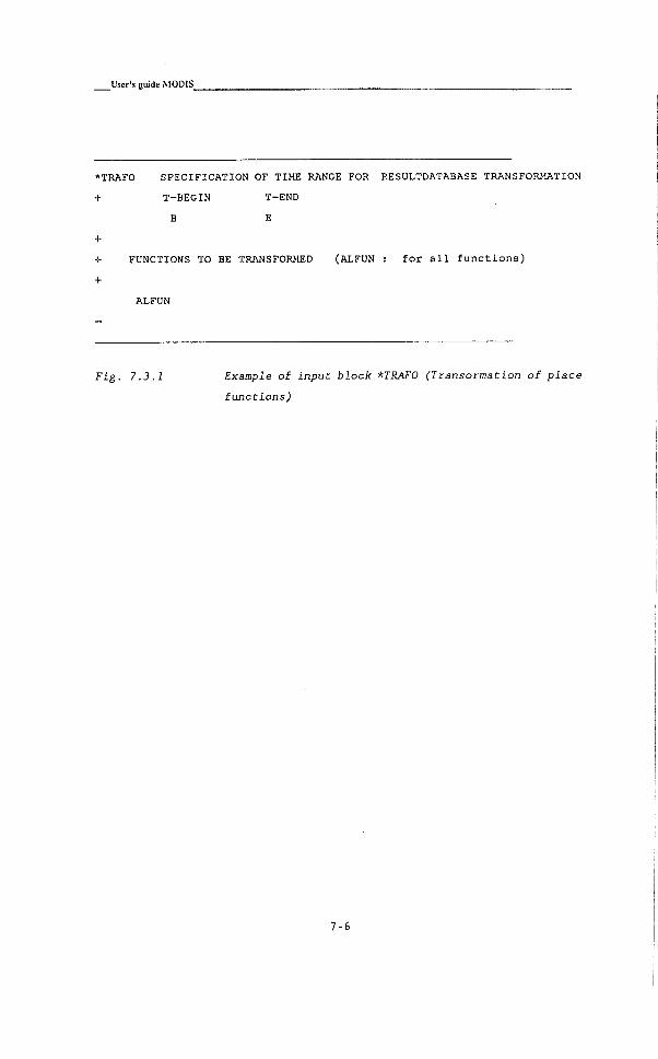
User's guide MODIS_
*TRAFO SPECIFICATION OF TIME RANGE FOR RESULTDATABASE TRANSFORMATION
+ T-BEGIN T-END
B E
+
+ FUNCTIONS TO BE TRANSFORMED (ALFUN : f o r a l l f u n c t i o n s )
+
ALFUN
Fig. 7.3.1 Example of input block *TRAFO (Transormation of place
functions)
7-6

Result database
7.4 Investigation of content
The t h i r d input block, contains switches i n the usual way, f o r
i n v e s t i g a t i n g the contents of the SST and RTF f i l e and the f i v e GRF
f i l e s . The input block i s i d e n t i f i e d by:
•CONT - INVESTIGATE CONTENTS OF RESULT DATA BASE
+ TIME FUNCTIONS
+ SST RTF
Where f o r each f i l e the character Y (yes) or N (no) can be given
i n d i c a t i n g wheter or not to check the contents of the s p e c i f i c f i l e .
The input block i s followed by the f o l l o w i n g comment l i n e s :
+ PLACE-FUNCTIONS
+ GRF-1 GRF-2 GRF-3 GRF-4 GRF-5
Again, f o r each GRF-# f i l e the character Y (yes) or N (no) can be given
i n d i c a t i n g wheter or not to check the content of the s p e c i f i c f i l e . The
input segment i s closed by a l i n e containing the character s t r i n g
•END i n the f i r s t columns. An example of the input block «CONT i s shown
i n Fig. 7.4.1
•CONT INVESTIGATE CONTENTS OF RESULT-DATABASE
+ TIME FUNCTIONS
+ SST RTF
Y Y
+ PLACE-FUNCTIONS
+ GRF-1 GRF-2 GRF-3 GRF-4 GRF-5
Y N N N Y
•END
Fig. 7.4.1 Example of input block *CONT (content check)
7-7


8 Model results, tables
8.1 Introduction
A s e l e c t i v e access to the computed r e s u l t s can be made w i t h the help of
subsystem MODRES. I n t h i s way only the r e s u l t s which are of d i r e c t
i n t e r e s t to the user are p r i n t e d or shown on the s c r e e n . A f i r s t
s e l e c t i o n i s made by the u s e r i n the subsystem MODCOM. There i t i s
s p e c i f i e d which computed r e s u l t s and other data are to be w r i t t e n to the
r e s u l t data base, e i t h e r i n the form of f u n c t i o n s of time or as f u n c t i o n s
of p l a c e . I n t h i s subsystem (MODRES) a f u r t h e r s e l e c t i o n i s made and the
form i s s p e c i f i e d i n which the f u n c t i o n s are to be produced on p r i n t
output.
The u s e r can s e l e c t f o r each s e t of f u n c t i o n s the page format by g i v i n g
the number of c h a r a c t e r s per l i n e and the number of l i n e s per page. I n
t h i s way the output can be t a i l o r e d to any output medium.
For each f u n c t i o n some general i n f o r m a t i o n can be given, such as v a r i a b l e
u n i t s , e t c . as w e l l as the format i n which the data are to be p r i n t e d .
Functions are p r i n t e d i n v e r t i c a l columns of u s e r - s p e c i f i e d width. The
number of f u n c t i o n s that can be p r i n t e d i n p a r a l l e l i s c a l c u l a t e d from
the page width and the number of c h a r a c t e r s needed f o r each i n d i v i d u a l
f u n c t i o n . For each s e t of f u n c t i o n s p r i n t e d a c c e s s can be made to 5
d i f f e r e n t G R F - f i l e s ( g e n e r a l r e s u l t f i l e s , which are the f i l e s with
f u n c t i o n s arranged i n the format r e q u i r e d f o r subsystem MODRES or
MODPLT).
Th i s enables the user to compare i n one p r i n t o u t , f o r example, measured
r e s u l t s w i t h r e s u l t s from computations. One f u n c t i o n can be p r i n t e d
s e v e r a l times. T h i s i s p a r t i c u l a r l y u s e f u l when i n the f i r s t column, f o r
example, time, x, g r i d point numbers or g r i d p o i n t names are d i s p l a y e d ,
a g a i n s t which the r e s u l t f u n c t i o n v a l u e s are s e t i n the subsequent
columns.
8-1

User's guide MODIS
Except f o r time, these v a l u e s are not a u t o m a t i c a l l y a v a i l a b l e on the GRF-
f i l e s . They have to be produced i n MODCOM i n the same way as, f o r
example, water l e v e l s and d i s c h a r g e s are produced (see par. 8.9).
Some t y p i c a l forms of output t h a t can be designed with MODRES a r e :
p r i n t i n g the r e s u l t s a t d i f f e r e n t g r i d p o i n t s as a f u n c t i o n of time;
comparing a t one g r i d p o i n t the measured r e s u l t s w i t h the r e s u l t s of
d i f f e r e n t c a l i b r a t i o n runs;
p r i n t i n g water l e v e l s a t d i f f e r e n t points along a branch a g a i n s t the
g r i d p o i n t names;
producing f o r each branch a ta b l e of g r i d point names w i t h x - v a l u e s
and g r i d p o i n t numbers.
Producing f o r each g r i d p o i n t operation performance parameters.
These parameters a re the d e l i v e r y performance r a t i o and the
op e r a t i o n e f f i c i e n c y . The d e l i v e r y performance r a t i o e x p r e s s e s to
which extend the a c t u a l water d e l i v e r y has met the intended water
d e l i v e r y during a c e r t a i n p e r i o d of time. The o p e r a t i o n e f f i c i e n c y
s p e c i f i e s which p a r t of the a c t u a l supply has been given
e f f e c t i v e l y .
The same k i n d of f u n c t i o n s can be represented on g r a p h i c a l output by
means of sub-system MODPLT which produces graphs and p l o t s .
Place f u n c t i o n s are produced per route. I n the output i t i s p o s s i b l e to
concatenate 5 d i f f e r e n t f u n c t i o n s . T h i s enables the user to p r i n t r e s u l t s
of up to f i v e routes i n sequence i n one ta b l e .
The input of subsystem MODRES, i s given i n the input f i l e named
RESIN.DAT. T h i s f i l e has been organized i n one segment of three b l o c k s :
•*PRI - g i v i n g names of f i l e s to be used and paper format
s p e c i f i c a t i o n ;
* B L K - g i v i n g the s p e c i f i c a t i o n s of each s e t of f u n c t i o n s to be
p r i n t e d .
*OPP - g i v i n g the s p e c i f i c a t i o n s of g r i d p o i n t s of which Operation
Performance Parameters have to be determined.
8-2
Model results, tables.
The blncVt-q "BLK and -"OPP can be r e p e a t e d an u n l i m i t e d number o f tinges o r
simply skipped i f not used.
8-3
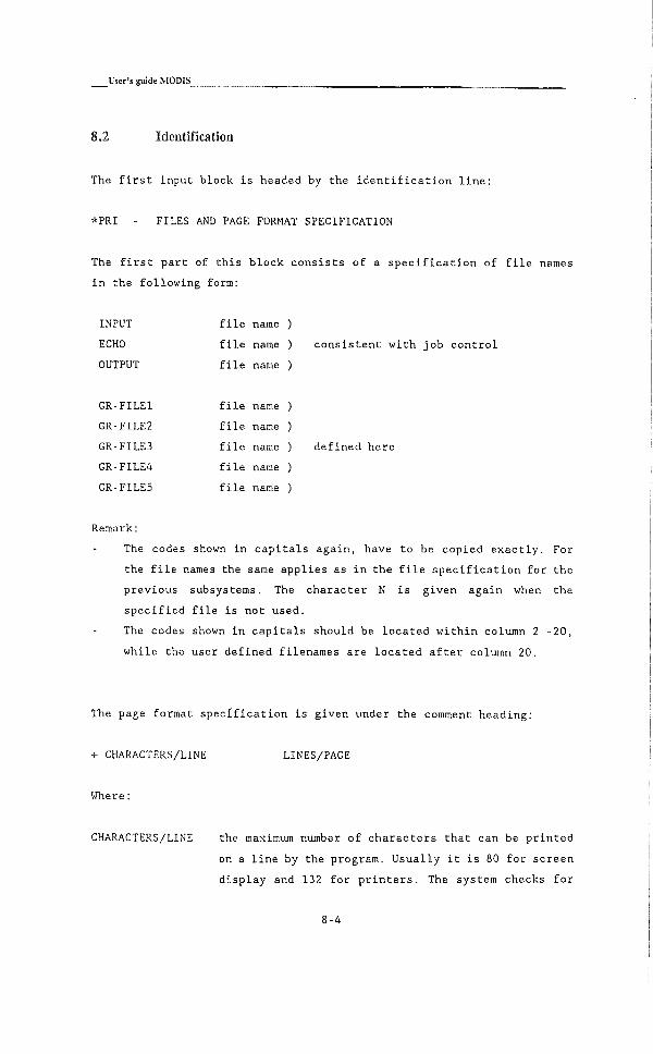
L'ser's guide MODIS
8.2 Identification
The f i r s t input block i s headed by the i d e n t i f i c a t i o n l i n e :
*PRI - FI L E S AND PAGE FORMAT SPECIFICATION
The f i r s t p a r t of t h i s b l o c k c o n s i s t s of a s p e c i f i c a t i o n of f i l e names
i n the f o l l o w i n g form:
INPUT f i l e name )
ECHO f i l e name ) c o n s i s t e n t with j ob c o n t r o l
OUTPUT f i l e name )
GR - F I L E l f i l e name )
GR-FILE2 f i l e name )
GR-FILE3 f i l e name ) def i n e d here
GR-FILE4 f i l e name )
GR-FILE5 f i l e name )
Remark:
The codes shown i n c a p i t a l s again, have to be copied e x a c t l y . For
the f i l e names the same a p p l i e s as i n the f i l e s p e c i f i c a t i o n f o r the
previous subsystems. The c h a r a c t e r N i s given again when the
s p e c i f i e d f i l e i s not used.
The codes shown i n c a p i t a l s should be l o c a t e d w i t h i n column 2 -20,
wh i l e the user d e f i n e d filenames are l o c a t e d a f t e r column 20.
The page format s p e c i f i c a t i o n i s given under the comment heading:
+ CHARACTERS/LINE LINES/PAGE
Where:
CHARACTERS/LINE the maximum number of c h a r a c t e r s t h a t can be p r i n t e d
on a l i n e by the program. U s u a l l y i t i s 80 f o r s c r e e n
d i s p l a y and 132 for p r i n t e r s . The system checks f o r
8-4
Model results, tables
each s e t o f f u n c t i o n s t h e r e q u i r e d nuraber o f
c h a r a c t e r s by adding up, for each f u n c t i o n , the
maximum of p r i n t i n g format and f u n c t i o n t i t l e . When
the c a l c u l a t e d v a l u e exceeds the one s p e c i f i e d , an
e r r o r message w i l l be produced;
LINES/PAGE the maximum number of l i n e s per pag e , u s u a l l y 60 or 64.
The system w i l l a u t o m a t i c a l l y s k i p to the next page as
soon as t h i s number of l i n e s has been p r i n t e d .
The l a s t data of t h i s i nput block are given under the comment l i n e
+ SUMMARY OUTPUT ONLY ? (Y/N)
where e i t h e r Y ( e s ) or N(o) can be given.
When Y i s s p e c i f i e d , only summary output i s given, c o n s i s t i n g of a t i t l e
page and a f u n c t i o n summary of a l l the f u n c t i o n s of the s e t , c o n t a i n i n g
the f o l l o w i n g c h a r a c t e r i s t i c s per f u n c t i o n :
- f u n c t i o n column number;
- f u n c t i o n t i t l e ;
- f u n c t i o n t e x t of 40 c h a r a c t e r s ;
- the s p e c i f i e d u n i t (e.g. m3/s);
- the maximum and minimum v a l u e s of the f u n c t i o n ;
- the number of elements i n the f u n c t i o n ;
When N i s given a l s o the f u n c t i o n t a b l e s are p r i n t e d , where each f u n c t i o n
s p e c i f i e d i s presented i n a column, headed by the f u n c t i o n t i t l e .
The input f o r block *PRI i s terminated again by g i v i n g the c h a r a c t e r
i n the f i r s t column of a c l o s i n g l i n e .
An example of input block *PRI i s given i n F i g . 8.2.1.
8-5

User's guide MODIS
*PRI
+
SPECIFICATION OF FILES AND PAPER-FORMAT
USED DATA SETS
INPUT
ECHO
OUTPUT
G R - F I L E l
GR-FILE2
GR-FILE3
GR-FILE4
GR-FILES
RESIN.DAT
RESECH.DAT
RESOUT.DAT
USPLF.UNF
N
N
N
USTIF.UNF
CHARACTERS/LINE LINES/PAGE
132 60
SUMMARY OUTPUT ONLY (Y/N)
N
Fig. 8.2.1 Example of input block *PRI (Identification of files and
print format)
8-6

Model results, tables
8.3 Spccincalioii of labulalcd output
Input i s continued by g i v i n g one or more s p e c i f i c a t i o n s f o r s e t s of
f u n c t i o n s to be p r i n t e d , each preceded by the i d e n t i f i c a t i o n l i n e :
*BLK - SPECIFICATION OF AN OUTPUT SET
+
+ BLOCK-TITLE
a s t r i n g of 40 c h a r a c t e r s can be given d e s c r i b i n g a g e n e r a l
c h a r a c t e r i s t i c of the s e t of f u n c t i o n s . T h i s t i t l e w i l l be reproduced on
the output f i l e .
F u n c t i o n s p e c i f i c a t i o n s are given f o l l o w i n g the comment l i n e :
+ COLNO GR-FILE FORMAT UNITS F F F F F
Vhere:
COLNO The s e q u e n t i a l column number where the r e s u l t s w i l l be
p r i n t e d . U s u a l l y they a re i n sequence of the data l i n e s ,
though t h i s i s not n e c e s s a r y .
GRF-FILE The GRF f i l e number where the f u n c t i o n should be read
from. The number can va r y from 1 to 5, assuming t h a t the
corresponding f i l e has been as s i g n e d i n the *PRI-block.
FORMAT The format to be used during p r i n t i n g of the r e s u l t
v a l u e s . T h i s i s given i n standard FORTRAN n o t a t i o n . The
format depends on the f u n c t i o n type. U s u a l l y the d e f a u l t
value can be s p e c i f i e d . The system then assumes as formats
A, 14 or F8.2 r e s p e c t i v e l y f o r the v a r i a b l e types
c h a r a c t e r , i n t e g e r and r e a l .
UNITS A c h a r a c t e r s t r i n g can be given here r e p r e s e n t i n g the
u n i t s of the v a l u e s , e.g. ra^/s.
F Up to 5 f u n c t i o n t i t l e s can be given f o r each column.
During p r i n t i n g they w i l l be concatenated and p r e s e n t e d as
one s i n g l e f u n c t i o n column. I n t h i s way i t i s p o s s i b l e to
8-7

User's guide M0D1S_
s p e c i f y s e v e r a l p l a c e f u n c t i o n s i n d i f f e r e n t branches as
a route through the channel network.
I f d u ring p r o c e s s i n g the *BLK-input block, a f a t a l e r r o r i s encountered
output p r o d u c t i o n s t o p s , a l s o f o r the b l o c k f o l l o w i n g tha t s p e c i f i c i n put
b l o c k . Each b l o c k i s terminated again w i t h a c l o s i n g l i n e w i t h the "-"
symbol i n the f i r s t column. An example of input b l o c k *BLK i s given i n
F i g . 8.3.1.
*BLK SPECIFICATION OF PRINT OUTPUT SET
+
+ BLOCK T I T L E
WATER LEVELS
+
+
+COLNO GR-FILE FORMAT UNITS FUNCTION FUNCTION FUNCTION FUNCTION
1 5 // D;H:M:S TIME
2 - # ...M.. H-GIO
3 - // - H-Gll
4 - // - H-G12
5 - # - H-G13
6 - # - H-G14
7 - # - H-G15
8 - # - H-G16
9 - i? - H-G17
10 - # - H-G18
Fig. 8.3.1 Example of Input block *BLK
Model results, tables.
8.4 Operation performance parameters
Input can be continued by g i v i n g one or more s p e c i f i c a t i o n s of the g r i d
p o i n t s of which O p e r a t i o n Performance Parameters have to be c a l c u l a t e d .
Not only the o p e r a t i o n performance parameters a t the i n d i v i d u a l g r i d p o i n t
can be c a l c u l a t e d , but a l s o o p e r a t i o n performance parameters of the t o t a l
system can be c a l c u l a t e d .
" S ing le o f f t akes
For the e v a l u a t i o n of the si m u l a t e d water d i s t r i b u t i o n to an i n d i v i d u a l
o f f t a k e , two o p e r a t i o n performance parameters are defined. The f i r s t one
i s c a l l e d the D e l i v e r y Performance R a t i o (DPR) and s p e c i f i e s the ext e n t
to which an o f f t a k e r e c e i v e s i t s intended supply. The second one i s
c a l l e d the o p e r a t i o n e f f i c i e n c y (e^,) and s p e c i f i e s the amount of water
l o s t by i n a p p r o p r i a t e a l l o c a t i o n of the water to an o f f t a k e . I n formulae
these parameters read:
DPR - - 1 • 1 0 0 % 8.1
- _ 1 o 100%
Where:
DPR - D e l i v e r y performance r a t i o (-)
- Operation e f f i c i e n c y (-)
- Volume e f f e c t i v e l y d e l i v e r e d (m^)
VJ - Volume intended to be d e l i v e r e d (m^)
Vg - Volume a c t u a l l y d e l i v e r e d (m'')
As can be r e a d from the presented formulae, three volumes of water are
d i s t i n g u i s h e d : An intended volume to be s u p p l i e d , an a c t u a l volume
s u p p l i e d , and an e f f e c t i v e volume s u p p l i e d .
• C o m p l e t e system
To e v a l u a t e the o p e r a t i o n a l performance of a c a n a l system i n c l u d i n g a l l
i t s o f f t a k e s , o v e r a l l performance parameters are needed. The o v e r a l l
D e l i v e r y Performance R a t i o i s c a l c u l a t e d by a weighed average of the DPR
of the i n d i v i d u a l o f f t a k e s and reads:
8 - 9
L'ser's guide MODIS
DPR^^ 8.3
EV,. E ^ M
Where DPR^^arall -̂̂ the o v e r a l l D e l i v e r y Performance R a t i o , „ i s the
e f f e c t i v e volume r e c e i v e d by o f f t a k e n (m') , „ i s the intended volume
to be r e c e i v e d by o f f t a k e n (m^) , and p i s the number of o f f t a k e s
involved.
The o v e r a l l operation e f f i c i e n c y i n c o r p o r a t e s the o p e r a t i o n a l l o s s e s of
the i n d i v i d u a l o f f t a k e s , the l o s s e s due to f i l l i n g up the c a n a l to i t s
o p e r a t i o n a l l e v e l , and the leakage l o s s e s and or s p i l l l o s s e s i f these
occur. I n formula i t reads,
E / , . 8.4
Where eo^overail I s the o v e r a l l o p e r a t i o n e f f i c i e n c y , ^ ^ t ^ j i s the a c t u a l
intake volume a t the head of the main c a n a l (m^) , V, „ i s the e f f e c t i v e
volume r e c e i v e d by o f f t a k e n (m^) , and p i s the nuraber of o f f t a k e s
involved.
The o v e r a l l d e l i v e r y performance r a t i o becomes equal to the o v e r a l l
o p eration e f f i c i e n c y i f the sum of intended volumes i s equal to the
volume taken i n . I n t h a t case the o v e r a l l performance of the c a n a l system
can be c h a r a c t e r i z e d by one s i n g l e f i g u r e .
• Seepage losses
Although seepage l o s s e s w i l l always occur i n t h i s study no s p e c i a l
a t t e n t i o n has been p a i d to i t . Nonetheless i t i s v e r y w e l l p o s s i b l e to
in c o r p o r a t e seepage l o s s e s i n the model by e x t r a c t i n g c e r t a i n amounts of
water a t c e r t a i n l o c a t i o n s . The l o s s e s due to seepage can be accounted
fo r by the o v e r a l l o peration e f f i c i e n c y only.
For a more d e t a i l e d d i s c u s s i o n of the o p e r a t i o n performance parameters,
r e f e r e n c e i s made to chapter 11.
8-10

Model results, tables.
I n p u t
The i d e n t i f i c a t i o n l i n e i s read:
*OPP
+ Block T i t l e
A name of the output b l o c k can be s p e c i f i e d up to 40 c h a r a c t e r s long.
T h i s name i s copied to the header of the output f i l e .
F u n c t i o n s p e c i f i c a t i o n s a re given f o l l o w i n g the comment l i n e :
+ LINNO G R - f i l e Name Tbegin Tend Qtarget Qmax Qrain
Where
LINNO
GR-FILE
NAME
TBEGIN
TEND
QTARGET
Li n e number u s u a l l y s t a r t i n g a t 1 .
The G R - f i l e number where the f u n c t i o n should be read from.
U s u a l l y number 5 i s chosen, as i n t h i s f i l e water l e v e l s
and d i s c h a r g e s are s t o r e d .
Name of g r i d p o i n t of which the OPP must be c a l c u l a t e d .
The s p e c i f i e d name of the g r i d p o i n t must a l r e a d y be
defi n e d i n COMIN.DAT, otherwise no data have been s t o r e d
of t h a t g r i d p o i n t .
S t a r t i n g time of determination of the OPP. TBEGIN must be
given as a time s t r i n g i n d:h:m:s n o t a t i o n . When a "B" i s
given the c a l c u l a t i o n of the OPP s t a r t s with the f i r s t
time s p e c i f i e d i n subsystem MODCOM. When a "-" c h a r a c t e r
i s given the Btime i s s e t equal to Btime of the above
input l i n e .
End time i s the time s p e c i f y i n g the end of the c a l c u l a t i o n
of the OPP. S i m i l a r with TBEGIN, TEND must be given e i t h e r
i n d:h:m:s n o t a t i o n or with the c h a r a c t e r E. When "E" i s
given TEND i s equal to the l a s t time of the G R - F i l e . When
a "-" c h a r a c t e r i s given Tend i s s e t equal to Tend of the
previous input l i n e .
Qtarget i s the t a r g e t or intended v a l u e o f the d i s c h a r g e .
The model compares the a c t u a l d e l i v e r e d d i s c h a r g e w i t h the
8-11

User's guide MODIS
intended d i s c h a r g e to c a l c u l a t e the o p e r a t i o n performance
parameters.
Qtmax Maximum a c c e p t a b l e flow r a t e . Qtmax can be given e i t h e r as
a f i g u r e or as a percentage of the o f f s e t of the t a r g e t
d i s c h a r g e . I n the l a t t e r case the percentage s i g n "%" must
be p l a c e d d i r e c t l y a f t e r the d i g i t s . So, i f 25% i s
s p e c i f i e d , the maximum allowable discharge i s equal to;
Qtarget + 25% of Q t a r g e t . I f the a c t u a l d i s c h a r g e exceeds
the maximum di s c h a r g e the d i f f e r e n c e between the a c t u a l
and maximum a c c e p t a b l e discharge i s c o n s i d e r e d as a l o s s .
Qtmin Minimum a c c e p t a b l e d i s c h a r g e . The same n o t a t i o n s can be
used as f o r Qtmax, e i t h e r a percentage or a number. So, i f
25% i s s p e c i f i e d , the minimum allowable d i s c h a r g e i s equal
to; Qtarget - 25% of Qtarget. I f the a c t u a l d e l i v e r e d
d i s c h a r g e drops below the minimum disc h a r g e the a c t u a l
d e l i v e r e d d i s c h a r g e w i l l be considered to be a d i s c h a r g e
l o s s .
Total performance
I t i s a l s o p o s s i b l e to e v a l u a t e the t o t a l performance of the c a n a l
system. I n t h a t case, the i n d i v i d u a l o f f t a k e s have to be s p e c i f i e d f i r s t
i n the i n p u t block OPP. The l a s t l i n e of the input block *OPP should then
read:
+ LINNO G R - f i l e Name Tbegin Tend T o t a l
Where LINNO, G R - f i l e , Name, Tbegin and Tend remain the same.
Under T o t a l the word TOTAL should be given.
The Name to be s p e c i f i e d i s the name of the g r i d - p o i n t where the
d i s c h a r g e i s taken i n . T h i s g r i d - p o i n t i s used to c a l c u l a t e the V^^i^t^e
of Eq. ( 8 . 4 ) . A l l the proceeding points are i n c o r p o r a t e d i n the
computation of the o v e r a l l performance.
The input b l o c k i s c l o s e d as u s u a l by a l i n e c o n t a i n i n g the "-" c h a r a c t e r
8-12
Modd results, tables_
i n the f i r s t column.
An example of the input b l o c k "*OPP" i s given i n F i g . 8.4.1.
*OPP
+ Block T i t l e
Operation Performance R a t i o ' s
+ LINNO G R - f i l e Name Tbegin Tend Qtarg e t Qtmax Qtmin
1 5 Q-Gll B 00:10:00:00 1.5 2.0 40%
2 - Q-G12 B - 1.5 25%
3 „ Q.G15 B - 1.5 1.95 0.75
4 _ Q-GIO B - TOTAL
*END
Fig. 8.4.1 Example of input format of block *OFP (operation
performance parameters)
8-13

L'ser's guide MODIS
8.5 Maxlmun mean and minimum values
Input can be continued by g i v i n g one or more s p e c i f i c a t i o n s o f the g r i d
p o i n t s a t which other o p e r a t i o n a l performance parameters have to be
c a l c u l a t e d than the DPR and eo. These other parameters were o r i g i n a l l y
used to e v a l u a t e water l e v e l s r a t h e r than d i s c h a r g e s but d i s c h a r g e s can
be e v a l u a t e d as w e l l . The parameters which are c a l c u l a t e d are the
maximum, minimum and mean v a l u e s during a c e r t a i n p e r i o d of time.
Furthermore, the percentage of time during which a minimum l e v e l has been
exceeded, and the percentage of time during which a maximum l e v e l has
been exceeded can be presented.
The i d e n t i f i c a t i o n l i n e i s read:
*MMM
+ Block T i t l e
A name of the output block can be s p e c i f i e d up to 40 c h a r a c t e r s long.
T h i s name i s copied to the header of the output f i l e .
F u n c t i o n s p e c i f i c a t i o n s are given f o l l o w i n g the comment l i n e :
+ LINNO G R - f i l e Name Tbegin Tend Htarget Hmax Hmin
I n p u t
Where
LINNO Li n e number u s u a l l y s t a r t i n g a t 1.
GR-FILE The G R - f i l e number where the f u n c t i o n should be read from.
U s u a l l y number 5 i s chosen, as i n t h i s f i l e water l e v e l s
and discharges are s t o r e d .
NAME Name of g r i d p o i n t of which the OPP must be c a l c u l a t e d .
The s p e c i f i e d name of the g r i d p o i n t must a l r e a d y be
defined i n COMIN.DAT, otherwise no data have been s t o r e d
of t h a t g r i d p o i n t .
TBEGIN S t a r t i n g time of dete r m i n a t i o n of the OPP. TBEGIN must be
8-14

Model results, tables.
g i v e n as a time s t r i n g i n d;h:m:s n o t a t i o n . Vhen a "B" i s
g i v e n the c a l c u l a t i o n of the OPP s t a r t s with the f i r s t
time s p e c i f i e d i n subsystem MODCOM. When a c h a r a c t e r
i s g i ven the Btime i s s e t equal to Btime of the above
i n p u t l i n e .
TEND End time i s the time s p e c i f y i n g the end of the c a l c u l a t i o n
of the OPP. S i m i l a r w i t h TBEGIN, TEND must be given e i t h e r
i n d:h:m:s n o t a t i o n or w i t h the c h a r a c t e r E. When "E" i s
given TEND i s equal to the l a s t time of the G R - F i l e . When
a "-" c h a r a c t e r i s given Tend i s s e t equal to Tend of the
pre v i o u s input l i n e .
HTARGET Htarget i s the t a r g e t or intended v a l u e of the di s c h a r g e .
The model only c o p i e s t h i s t a r g e t l e v e l to the output f i l e
i n order to f a c i l i t a t e easy comparison w i t h the mean
v a l u e .
Htmax Maximum a c c e p t a b l e water l e v e l . The t o t a l time during
which the a c t u a l l e v e l exceeds the maximum l e v e l i s
monitored. I n the output f i l e t h i s time d i v i d e d by the
s p e c i f i e d p e r i o d of time i s presented as a percentage
Htmin Minimum ac c e p t a b l e water l e v e l . I f the a c t u a l water l e v e l
drops below the minimum water l e v e l , the time of
exceedings i s monitored. I n the output f i l e , again t h i s
time i s presented as a percentage of the t o t a l time
c o n s i d e r e d .
The input block i s c l o s e d as u s u a l by a l i n e c o n t a i n i n g the "-" c h a r a c t e r
i n the f i r s t column. An example of the input b l o c k "*MMM" i s given i n
F i g . 8.5.1.
8-15
User's guide MODIS
*MMM
+ Block T i t l e
Maximum Minimum and mean v a l u e s
+ LINNO G R - f i l e Name Tbegin Tend
1 5 H-Gll B 00:10:00:00
2 - H-G12 B
3 - H-G15 B
*END
Fig. 8.5.1 Example of Input format of block *HHM (maximum minimum and
mean values) .
The complete input l i s t f o r sub-system MODRES i s terminated by an empty
l i n e c o n t a i n i n g "*END" i n the f i r s t columns.
Htarget Hmax Hmin
15.30 15.00 15.60
14.25 13.95 15.00
13.46 13.23 13.75
8-16

9 Model results, plots
9.1 Introduction
I t i s p o s s i b l e to present the r e s u l t s of a s i m u l a t i o n i n a graph or p l o t .
T h i s g r a p h i c a l subsystem i s c a l l e d HODPLT (MODel PLoTs). The input of
subsystem MODPLT i s s p e c i f i e d i n input f i l e which i s named PLTIN.DAT. The
input f i l e has been organized i n one segment of f i v e b l o c k s :
*PL0T s p e c i f i e s the f i l e names and p l o t t e r device to be used;
•"SIZE s p e c i f i e s the paper s i z e or format of the paper;
••̂ TEXT s p e c i f i e s some general t e x t to be p l o t t e d on the drawing;
•-•'AXES s p e c i f i e s the axes to be drawn, and the s c a l e s to be used;
•-LINS s p e c i f i e s che fu n c t i o n s Co be rep r e s e n t e d by a l i n e and the
l i n e code to be used;
The b l o c k s have Co be repeated i n the sequence as above f o r each new
drawing. T h i s can be done an u n l i m i t e d number of times.
9-1

User's guide MODIS
9.2 Identification
The f i r s C i n put block i s headed by the i d e n t i f i c a t i o n l i n e :
*PLOT - F I L E S AND OUTPUT SPECIFICATION
The f i r s t p a r t of t h i s b lock c o n s i s t s of a s p e c i f i c a t i o n of f i l e names
i n the f o l l o w i n g form:
INPUT
ECHO
OUTPUT
f i l e name \
f i l e name > c o n s i s t e n t with j ob c o n t r o l
f i l e name /
G R - F I L E l
GR-FILE2
GR-FILE3
GR-FILE4
GR-FILE5
f i l e name \
f i l e name |
f i l e name > defined here
f i l e name |
f i l e name /
"c o l no >- 2 : o l no >- 20
The codes shown i n c a p i t a l s have to be copied again e x a c t l y . For the f i l e
names the same a p p l i e s as i n the f i l e s p e c i f i c a t i o n f o r the prev i o u s sub
systems. The c h a r a c t e r N i s given again when the s p e c i f i e d f i l e i s not
used.
T h e r e a f t e r , the p l o t t e r device to be used i s given under the comment
heading:
PLOTTER DEVICE
9-2

Model results, plots
At present the a v a i l a b l e p l o t t e r d e v i c e s are l i s t e d :
CALCOMP
HP7475A
HERCULES
CCA
VGA
EGA
The l a s t four d e v i c e s are producing a colour graph on your s c r e e n . Of
course the p l o t t e r device should be chosen i n accordance w i t h your
g r a p h i c a l c a r t e.g He r c u l e s , VGA.
F i n a l l y , the t e x t font have to be s p e c i f i e d , under the heading:
+ TEXT FONT
The two p o s s i b l e t e x t f o n t s a r e :
- DRAFT
- FINAL
The input block i s c l o s e d a g a i n by g i v i n g the c h a r a c t e r i n the f i r s t
coluinn of a c l o s i n g l i n e .
9-3

User's guide MODIS
An example of the Input block *PLOT i s given i n F i g . 9.2.1
*PLOT - SPECIFICATION OF F I L E S AND PAPER-FORMAT
+ USED DATA SETS
INPUT PLTIN.DAT
ECHO PLTECH.DAT
OUTPUT PLTOUT.DAT
GR - F I L E l USPLF.UNF
GR-FILE2 N
GR-FILE3 N
GR-FILE4 N
GR-FILE5 USTIF.UNF
+ PLOTTER DEVICE
CALCOMP
VGA
EGA
+
+ TEXT FONT
FINAL
Fig. 9.2.1 Example of input block *PLOT
9-4

Mddtl results, plots
9.3 Specification of plot size
Input has to be continued by the a c t u a l s p e c i f i c a t i o n of a drawing. The
f i r s t i n p ut block of such a s p e c i f i c a t i o n i s * S I Z E w i t h i d e n t i f i c a t i o n
l i n e :
* SIZE - SPECIFICATION OF PLOT SIZE
The f i r s t i n p ut l i n e i s preceded by the comment l i n e :
+ PLOT SI Z E WIDTH HEIGHT
Where:
PLOT SIZE: s p e c i f i e s the paper format. U s u a l l y a standard s i z e
a c c o r d i n g to the A-norm w i l l be used (e.g. A4 or A 3 ) . One
can a l s o s e l e c t a number of times a c e r t a i n standard
format. For i n s t a n c e 3A4 s p e c i f i e s a paper format with
the h e i g h t of an A4 sheet and the width of 3 times an A4
s h e e t . A non-standard format can be s p e c i f i e d by U. I n
t h i s case the next data items on the l i n e w i l l be read, to
s p e c i f y the paper s i z e . The d e f a u l t v a l u e i s : A 4 .
WIDTH: s p e c i f i e s the width of the paper i n c e n t i m e t r e s i n case of
a non-standard paper s i z e . The d e f a u l t v a l u e i s : 21.0 (A4
w i d t h ) .
HEIGHT: s p e c i f i e s the h e i g h t of the paper i n c e n t i m e t r e s i n case
of a non-standard paper s i z e . The d e f a u l t v a l u e i s 29.7.
( A 4 h e i g h t ) .
The input b l o c k i s terminated again by g i v i n g the c h a r a c t e r i n the
f i r s t column of a c l o s i n g l i n e .
9-5

L'ser's guide MODIS
An example of the input b l o c k * S I Z E i s given i n F i g . 9.3.1
* S I Z E - PLOT SIZE
+
+ PLOT SIZE WIDTH HEIGHT
A3 #
A4 it U 29.7 21.0
Fig. 9.3.1 Example of inpuC block *PLOT
9-6
.Model results, plots
9.4 Specification of plot text
Input i s continued by input block *TEXT to s p e c i f y some g e n e r a l t e x t to
be p l o t t e d . The input s t a r t s with the i d e n t i f i c a t i o n l i n e
*TEXT - PLOT TEXT
+ HEIGHT XCO YCO TEXT
Where:
HEIGHT S p e c i f i e s the height of the c h a r a c t e r s when p l o t t e d . There
i s a d e f a u l t for each s t r i n g number.
XCO S p e c i f i e s the x-coordinate of the t e x t when p l o t t e d . There
i s a d e f a u l t value f o r each s t r i n g number.
YCO S p e c i f i e s the y-coordinate of the t e x t when p l o t t e d . There
i s a d e f a u l t value f o r each s t r i n g number.
TEXT S p e c i f i e s the text to be p l o t t e d . At maximum 10 t e x t
s t r i n g s can be s p e c i f i e d to be p l o t t e d on che drawing.
I f f o r a l l p o s i t i o n v a l u e s (XCO and YCO) d e f a u l t v a l u e s are used the 10
t e x t s t r i n g s are p o s i t i o n e d as i n F i g u r e 9.4.1. The sequence number i s
based on the sequence i n the input form. One can change t h i s sequence
however by us i n g the s p e c i f i c a t i o n POS<no> i n s t e a d of (XCO,YCO). I f the
p o s i t i o n i s s p e c i f i e d for in s t a n c e by P0S4 the d e f a u l t p o s i t i o n v a l u e s
are used f o r s t r i n g 4, independent of the sequence number i n the input
form.
The d e f a u l t v a l u e s f o r HEIGHT for the v a r i o u s s t r i n g s a r e :
s t r i n g no 1 2 3 4 5 6 7 8 9 10
h e i g h t i n cra 0.4 0.3 0.3 0.3 0.3 0.3 0.3 0.3 0.5 0.4
The i n p u t block *TEXT i s terminated again by g i v i n g the c h a r a c t e r '=' i n
the f i r s t column of a c l o s i n g l i n e .
9-7
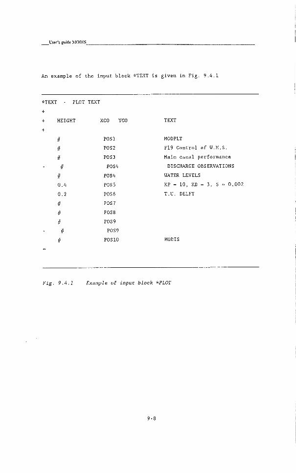
User's guide MODIS
An example of the input block *TEXT i s given i n F i g . 9.4.1
*TEXT
+
+
+
PLOT TEXT
HEIGHT
ë it it
it 0.4
0.2
it
XCO
POSl
POS 2
P0S3
P0S4
P0S4
POS 5
P0S6
P0S7
POS 8
P0S9
POS 9
POSIO
YCO TEXT
MODPLT
F19 Control of W.M.S.
Main c a n a l performance
DISCHARGE OBSERVATIONS
WATER LEVELS
KP - 10, KD - 3, S - 0.002
T.U. DELFT
MODIS
Fig. 9.4.1 Example of input block *PLOT
9-8

Model results, plots
9.5 Definition of axes
The nexc inpuC block of the form i s used Co define the axes and the s c a l e
used i n the drawing. The block i s s t a r t e d w i t h the i d e n t i f i c a t i o n l i n e :
*AXES - SPECIFICATION OF AXES
+
+ NR. START END LEN CRD PLACE TEXT
Where:
NR S p e c i f i e s the a x i s number. T h i s number i s used l a t e r on i n
input block *LINS to s p e c i f y what a x i s and s c a l e have to
be used to draw a c e r t a i n f u n c t i o n . Number 1 i s used to
d e f i n e the X - a x i s .
START Defines the o f f s e t v a l u e a t the beginning of the axes.
END Defines Che end v a l u e a t the end of the axes.
LEN Defines the l e n g t h of the axes on the paper i n cra. Thus
the s c a l e i s d e f i n e d by (END-START)/LEN.
GRD S p e c i f i e s whether a g r i d has Co be plocced or noc. I f 'Y' ,
u s u a l l y a v e r c i c a l g r i d i s drawn. I f iC i s used f o r che X-
axes a h o r i z o n c a l g r i d i s drawn. Defaulc value i s 'N'.
PLACE Defines Che p l a c e where Che axes have Co be ploCCed. Pos
s i b l e v a l u e s are 'L' or 'R'. For che X - a x i s Chis s p e c i
f i c a t i o n does not have a meaning, but a value has to be
given (e.g. XX). I f 'L' i s s p e c i f i e d , the a x i s i s p o s i
t i o n ed a t the l e f t end of the X - a x i s . I f 'R' i s s p e c i f i e d
the a x i s i s p o s i t i o n e d a t the r i g h t end. I t i s p o s s i b l e to
s p e c i f y 'L' or 'R' more then once. I n t h i s case the axes
are drawn next to each other. D e f a u l t v a l u e i s 'L'
TEXT Defines the CexC to be ploCCed. The d e f a u l c texC i s blank.
As u s u a l che inpuC block i s cerminaCed by a l i n e wich a '-' as the
c o n t r o l c h a r a c t e r .
9-9

L'ser's guide MODIS
An example of the input block * S I Z E i s given i n F i g . 9.5.1
*AXES
+
+
+ NR.
+
1
- 2
2
SPECIFICATION OF AXES
AXIS NR 1 I S THE X-AXIS
START END
00:00:00:00 00:09:00:00
0.0 25.0
109.0 111.0
LEN GRD PLACE TEXT
N - SIMULATION TIME
N L DISCHARGE IN M3/S
N L WATER LEVEL IN M
Fig 9.5.1 Example of input: block *PLOT
9-10

Model results, plots_
9.6 Function specification
Input i s continued by the l a s t input b l o c k needed to d e f i n e one drawing.
T h i s input b l o c k s t a r t s with the i d e n t i f i c a t i o n l i n e ;
*LINS - SPECIFICATION OF FUNCTIONS TO BE DRAWN
+
+ NUMBER GR CODE UNIT FUNCTIONS ( MAX. 5) + AXIS F I L E
Where;
NO. AXIS
GR-FILE
CODE
UNIT
FUNCTION
I s the a x i s number from input b l o c k *AXES to be used when
drawing the f u n c t i o n
I s the G R - f i l e number corresponding to input block *PLOT
from which the f u n c t i o n has to be r e t r i e v e d .
Defines the l i n e code to be used to r e p r e s e n t the funct
ion. P o s s i b l e v a l u e s are $1 to $2A corresponding to 24
d i f f e r e n t l i n e f o n t s . B e s i d e s t h a t , the user can define
i t s own l i n e font by s p e c i f y i n g two a r b i t r a r y c h a r a c t e r s .
T h i s w i l l generate a l i n e font of a continuous l i n e , con
t a i n i n g those two c h a r a c t e r s p e r i o d i c a l l y .
Defines a u n i t s t r i n g used i n the p l o t legend
Here the f u n c t i o n codes have to be g i v e n to be p l o t t e d .
More than one f u n c t i o n can be given, i f i t i s done f o r the
whole block. Then the f u n c t i o n s are concatenated.
The input block i s c l o s e d by a l i n e c o n t a i n i n g the symbol "-" i n the
f i r s t column. The complete input l i s t f o r sub-system MODPLT i s terminated
a g a i n by the l i n e c o n t a i n i n g the c h a r a c t e r s t r i n g "*END" i n the f i r s t
columns.
9-11

_User's guide M0D1S_
An example of the input block *LINS i s given i n F i g . 9.6.1
*LINS - SPECIFICATION OF LINES IN DRAWING
+
+ NUMBER GR CODE UNIT FUNCTIONS (MAX. 5)
+ AXIS F I L E
1 5 XX D:M:H:Y TIME
2 - 11 ..M... H-GM02.1
2 - 12 ..M... H-GM03.1
2 - 13 ..M... H-GM04.1
*END OF PLTDEF
Fig 9.6.1 Example of Input block *PLOT
9-12
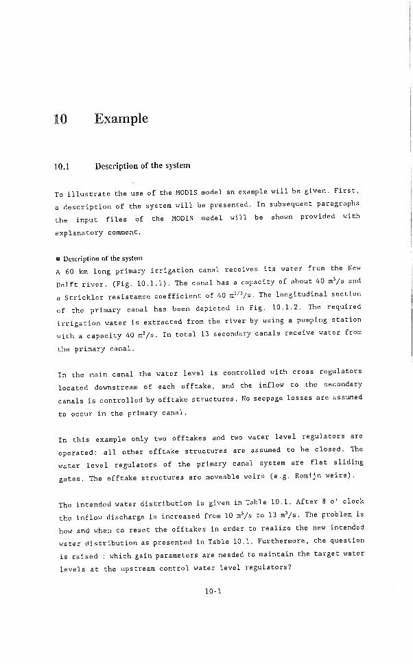
10 Example
10.1 Description of the system
To i l l u s t r a t e the use of the MODIS model an example w i l l be given. F i r s t ,
a d e s c r i p t i o n of the system w i l l be presented. I n subsequent paragraphs
the input f i l e s of the MODIS model w i l l be shown provided with
e x p l a n a t o r y comment.
• Description of the system
A 60 km long primary i r r i g a t i o n c a n a l r e c e i v e s i t s water from the New
D e l f t r i v e r . ( F i g . 10.1.1). The c a n a l has a c a p a c i t y of about 40 raVs and
a S t r i c k l e r r e s i s t a n c e c o e f f i c i e n t of 40 ra'^Vs• The l o n g i t u d i n a l s e c t i o n
of the primary c a n a l has been dep i c t e d i n F i g . 10.1.2. The r e q u i r e d
i r r i g a t i o n water i s e x t r a c t e d from the r i v e r by using a pumping s t a t i o n
w i t h a c a p a c i t y 40 raVs. I n t o t a l 13 secondary c a n a l s r e c e i v e water from
the primary c a n a l .
I n the main c a n a l the water l e v e l i s c o n t r o l l e d w i t h c r o s s r e g u l a t o r s
l o c a t e d downstream of each o f f t a k e , and the in f l o w to the secondary
c a n a l s i s c o n t r o l l e d by o f f t a k e s t r u c t u r e s . No seepage l o s s e s a re assumed
to occur i n the primary c a n a l .
I n t h i s example only two o f f t a k e s and two water l e v e l r e g u l a t o r s are
operated; a l l other o f f t a k e s t r u c t u r e s are assumed to be c l o s e d . The
water l e v e l r e g u l a t o r s of the primary canal system are f l a t s l i d i n g
g a t e s . The o f f t a k e s t r u c t u r e s are moveable weir s (e.g. Romijn w e i r s ) .
The intended water d i s t r i b u t i o n i s given i n Table 10.1. A f t e r 8 o' c l o c k
the i n f l o w d i s c h a r g e i s i n c r e a s e d from 10 mVs Co 13 raVs . The problem i s
how and when to r e s e t the o f f t a k e s i n order to r e a l i z e the new intended
water d i s t r i b u t i o n as presented i n Table 10.1. Furthermore, the question
i s r a i s e d ; which gain parameters are needed to maintain the t a r g e t water
l e v e l s a t the upstream c o n t r o l water l e v e l r e g u l a t o r s ?
10-1
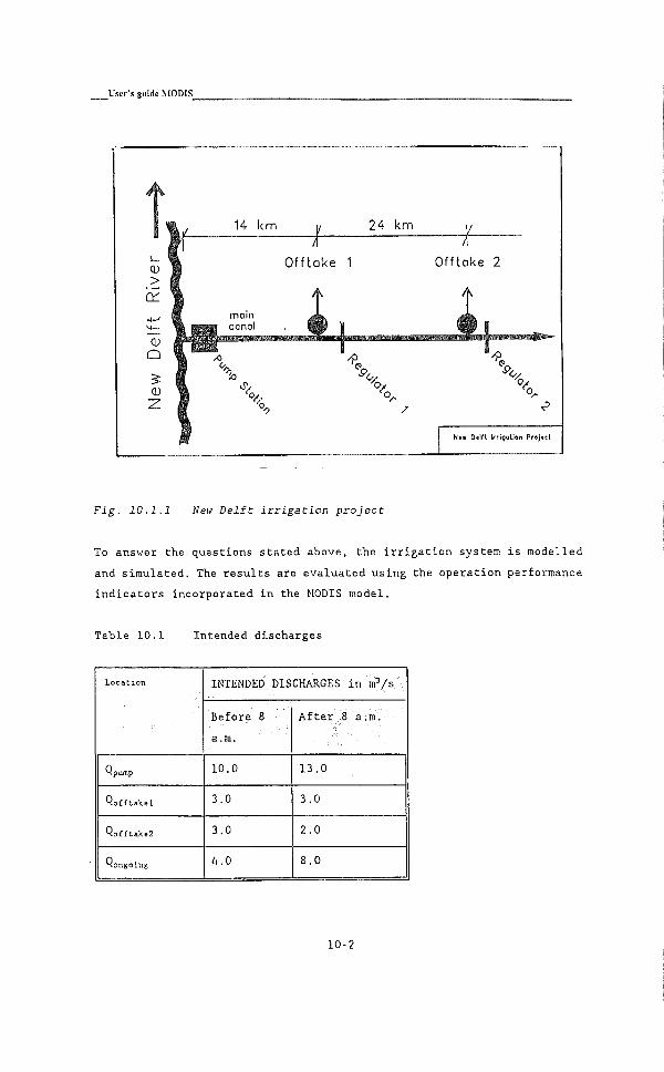
User's guide MODIS
Fig. 10.1.1 New Delft irrigation project
To answer the questions s t a t e d above, the i r r i g a t i o n system i s modelled
and s i m u l a t e d . The r e s u l t s are e v a l u a t e d u s i n g the ope r a t i o n performance
i n d i c a t o r s incorporated i n the MODIS model.
Table 10.1 Intended d i s c h a r g e s
Location INTENDED DISCHARGES i n rs?/s Location
Before 8
a.m..
A f t e r 8 a;ra.
Qpump 10.0 13.0
Qo££takBl 3.0 3.0
Qo£ft.a;<B2 3.0 2.0
Qongoing 4.0 8.0
10-2
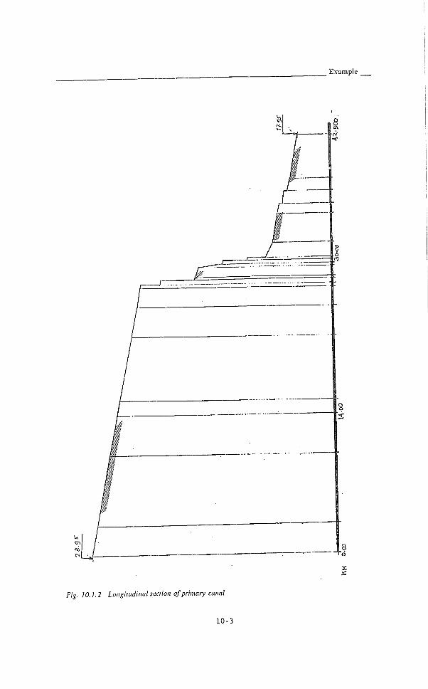
Exam
Fis- 10.1-2 Loiisiiudinal seaion of primary cannl
10-3

User's guide MODIS
10.2 Model Dermition
The input f i l e DEFIN.DAT of the model i s shown on the f o l l o w i n g pages.
Some a d d i t i o n a l comment on the input f i l e w i l l be l i s t e d . The remarks are
grouped by the input segments. ( A l s o r e f e r chapter 5 ) .
IDEN The data s p e c i f i e d i n Chis input segment can u s u a l l y be copied
from another e x i s t i n g input f i l e . With r e s p e c t to the s w i t c h e s
i t should be noted t h a t DEFINI which i s now on Y ( e s ) , have to
be put on "N" i f one wants to s t a r t the computation from a
p r e v i o u s computed steady s t a t e . The f i r s t time a computation i s
made, t h i s s w i t c h e s should be put on Y.
GRDDEF The s c h e m a t i s a t i o n of the system i s shown i n F i g . 10.2.1. The
a p p l i e d boundary c o n d i t i o n s a r e :
QT ( D i s c h a r g e t a b u l a t e d as a f u n c t i o n of time) w i t h the Table
name QINFLOW f o r the f i r s t node.
JW ( J u n c t i o n of water l e v e l s ) f o r the i n t e r n a l nodes
HC (Water l e v e l c o n s t a n t ) f o r the boundary notes. The water
l e v e l s are s p e c i f i e d lower than the s i l l l e v e l s of the
s t r u c t u r e s so t h a t f r e e flow through the s t r u c t u r e s o c c u r s .
S i x t r a p e z o i d a l c r o s s - s e c t i o n s have been defined.
G r i d p o i n t s have been d e f i n e d a t the beginning and end of each
branch, and/or upstream and downstream of each s t r u c t u r e . The
r e f e r e n c e l e v e l r e f e r s to the bottom l e v e l of the c a n a l .
ADDDEF 11 o r i f i c e have been d e f i n e d , they are f u n c t i o n i n g as water
l e v e l r e g u l a t o r s . The F - c o e f f i c i e n t of each o r i f i c e equals one
which i m p l i e s t h a t submerged flow i s assumed i f the downstream
l e v e l exceeds the gate opening h e i g h t . Only the PX p o s i t i v e
d i r e c t i o n has been d e f i n e d . R e v e r s a l flow w i l l be equal to
zero.
Two r e g u l a t o r s have been automated. For those r e g u l a t o r s the
gate opening h e i g h t has been g i v e n as a f u n c t i o n of LA ( L o c a l
Automatic) c o n t r o l , i n s t e a d of a f i x e d value. The name of the
c o n t r o l l e r s t h a t are used are CNTR3 and CNTRIO.
The o f f t a k e s t r u c t u r e s are w e i r s whereby the s i l l l e v e l i s
v a r i e d as a Tabulated f u n c t i o n of Time ( T T ) . The drowned flow
r e d u c t i o n c o e f f i c i e n t i s a T a b u l a t e d f u n c t i o n of the r a t i o
10-4
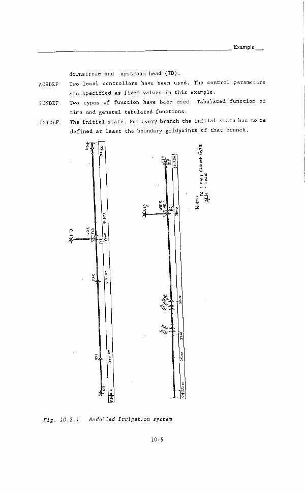
E x a m p l e
ACSDEF
FUNDEF
INIDEF
downstream and upstream head (TD).
Two l o c a l c o n t r o l l e r s have been used. The c o n t r o l parameters
are s p e c i f i e d as f i x e d v a l u e s i n t h i s example.
Two types of f u n c t i o n have been used: Tabulated f u n c t i o n of
time and g e n e r a l t a b u l a t e d f u n c t i o n s .
The i n i t i a l s t a t e . For every branch the i n i t i a l s t a t e has to be
d e f i n e d a t l e a s t the boundary g r i d p o i n t s of t h a t branch.
ore
.1
5- o
Fig. 10.2.1 Modelled Irrigation system
10-5

_User's guide MODIS_
Input file D E F I N . D A T
RUN-IDENTIFICATION
RUN-DESCRIPTION («0 CHARS.); Hew D e l f t i r r i g a t i o n p r o j e c t
<.. .>
RUNCOOE : March 1991
EXECUTED BY
DATASET (FILEHAHES)
INPUT DEFIN.DAT <JCL-HOOIFY)
ECHO DEFECH.DAT "
OUTPUT DEfOUT.DAT "
HODEIDB USMDB.UNF
SST-FILE USSST.UNF
•SUIT RUN-SWlTCHES
Y-YES N-NO ((-DEFAULT SETTING
+ NEUHODDB WRMODDB DEFALL
Y Y N
+ DEFNET DEFGRD
Y Y
+ OUTNET OUTGRD
Y Y
DEFFUN DEFINI
OUTFUN OUTINI
Y Y
OUTALL 0E8UCOUT FREE
N N #
DEFLAT
Y
OUTLAT
Y
FREE
#
DEFSTRUC DEFACS
Y Y
OUTSTRUC FREE
Y It
•END o f IDNDEF
•NODE D e f i n i t i o n s o f nodes
+NAHE TYPE CONNECTED BRANCHES Boundary Condi t i o n
v a l u e / r e f e r e n c e
NO QT BPl QINFLOW
N l JW BPl BS3 BP2
NS3 HC BS3 28.0
N2 JW BP2 BS9 BP3
NS9 HC BS9 19.0
N3 HC BP3 18.40
10-6

BRAM D e f i n i t i o n o f branches
HAHE BEGIN-NOOE END-NODE
BPl NO N l
BS3 N l NS3
BP2 N l N2
BS9 N2 NS9
BP3 N2 N3
END
TRAP T r a p e z o i d a l c r o s s - s e c t i o n s
+ NAME REFNCE BUESNQ Res
+ c o e f f
CO 0.0 1. 0 «O
C l 0.0 1, ,0 «0
C2 0.0 1 ,0 «0
C3 0.0 I .0 «0
C« 0.0 1 .0 «0
C5 0.0 1 .0 40
•GRID DEFINITION OF GRIDPOINTS
+ GRIDPOINT CROSS-SEC BRANCHE
name name name
GO CO BPl
Gl - -
GIR C l
G2 -
G2R C2
G3L . G3 C3 BP2
G3R C3 BP2
G4 C3 BP2
G4R C4
GS - -
G5R - -
G6 - -
G6R - -
G7 - -
G7R - -
G8 - •
G6R - -
G9 -
G9R -
GIOL -
GIO C4 BP3
GIOR BP3
G i l - BP3
G12
X-BEGIH X-ENO DX-HAX
0.0 140OO, ,0 1000.0
0.0 100, ,0 100.0
14000.0 38000 .0 1000.0
0.0 100 .0 100.0
38000.0 42500 .0 1000.0
BOTWIDTH SIOESLOPE Hmax
12.0 2.0 3.98
10.8 2.0
10.4 2.0
9.6 2.0
7.8 2.0
7.2 2.0
X-COORDINATE REF. LEVEL
t h e branch SI u n i t
0, 0 28.95
2995, ,0 28.65
3000, ,0 -
9995 ,0 27.95
10000, ,0 -
14000 ,0 27.55
14000, ,0 -
14005 ,0 -
21995 .0 26.75
22000 .0 -
27295 .0 26.22
27300 .0 25.15
27595 .0 25.12
27600 .0 23.40
29295 .0 23.10
29300 .0 21.90
29595 .0 21.65
29600 .0 20,65
29995 .0 20.55
30000 .0 19.64
38000 .0 18.40
38000 .0 18.40
38005 ,0 „
42495 .0 17.95
42500 ,0 16,95
10-7

User's guide MODIS_
GS3 C5 BS3 0.0 27.55
0S3E = - 100.0 27.50
GS9 C5 BS9 0.0 18.40
GS9E - - 100.0 18.35
'END OF GRDOEF
*0R1F
+ NAHE BRANCH X-COORD DIR F Ce u B z Y
FSl BPl 2998. 0 PX 1.0 1.0 0.63 10 28.65 0.30
FS2 BPl 9998. 0 - - - - = 27.95 0.55
FS3 BP2 14002. 0 - - - •= - 27.55 LA$CNTR3
fS4 BP2 21998. 0 - - - = 6 26.75 0.90
FS5 BP2 27298. 0 - 26.22 0.50
FS6 BP2 27598. 0 - - - - 25.12 0.53
FS7 29298. 0 - - 23.10 0.53
FS8 = 29598. 0 - - - - 21.85 0.53
FS9 = 29998. 0 - - = = 20.55 0.55
FSIO BP3 38002. 0 _ - - 5 18.40 LASCNTRIO
F S l l BP3 42498. 0 •= - = 17.95 0.50
*WEIR
+ NAHE BRANCH X-COORD DIR F Ce u B 2
WS3 BS3 5. 0 PX OTSFREO 1.0 1.5 12.0 TTSOFFl
WS9 BS9 5. 0 PX = 1.5 12.0 TT$0FF2
"END o f ADODEF
*AULC AUTOMATIC LOCAL CONTROL
+
+ NAHE CONTROL TYPE I n i v a l TARGET Kp Ki Kd SPEED HIN MAX
CNTR3 PID UC 0.23 30.15 -3.0 -1.8 0.5 0.5 0.0 2.0
CNTRIO PID UC 0.34 20.17 -3.0 -1.8 0.5 1.5 0.0 2.0
*END o f a u t o m a t i c c o n t r o l l e r s
*TTIM TABULATED FUNCTIONS OF TIME
+
NAHE OINFLOW OFFl 0FF2
+
00:00:00:00 10.0 29.872 19.892
00:07:59:00 - = =
00:08:00:00 13.0 29.872 19.97
05:00:00:00 = = •
10-8

Example
•TGFU
+
NAHE FRED
+ ( h 2 - z ) / ( h l - z ) Drowned f l o w
+ r e d u c t i o n f a c t o r
0.000 1.00
0.667 1.00
0.800 0,75
0.900 0.55
1.000 0.00
10.0 0.00
«EHD of fUHDEF
INSI D e f i n i t i o n o f i n i t i a I s t a t e o f c a n a l s y s tem
BRANCH G r i d P o i n t TYPE VAL/REF TYPE VAL/
H Q
BPl GO C 31.93 C 0,0
Gl - - -
GIR - 30.67 - -
G2 - = -
G2R - 30.15 - •
- G3L - - -
BS3 GS3 - - -
GS3E - -
BP2 G3 - - - -
- G3R - 29.55 - -
- - - -
C R - 28. 18 -
G5 - - - -
G5R - 27,08 - -
G6 - - - -
G6R - 25,06 - -
G7 - - - •
G7R - 23.81 - -
Ge - - - •
G8R - 22.51 - -
• G9 - - - -
G9R - 20.19 -
GIOL - - - -
BP3 GIO - - - -
BP3 GIOR - - -
. G12 - - - -
BS9 GS9 - - - -
GS9E 19.40 -
•END OF INIDEF
10-9

L'ser's guide MODIS
10.3 Model computation
Ths input f i l e COMIN.DAT of the subprogram MODCOM i s shown on the
f o l l o w i n g pages. For more information about the input data reference i s
made t o chapter 6.
Only one remark i s made about the input block *TIME. I n the f i r s t
computation, the SST (System State Time) f i l e should be on INIDEF which
implies t h a t the i n i t i a l state defined i n DEFIN.DAT i s read and used as
the i n i t i a l s t a t e .
I f the Steady s t a t e switch of input block *SWIT has been put on Y(es) a
new i n i t i a l s t a t e has been generated by the model and the SST could be
set on PERM (permanent stat e ) f o r the next computations. To save the
i n i t i a l s t a t e generated by the model the STEADÏ STATE switch should be
put on N(o) and i n the input f i l e DEFIN.DAT the DEFINI switch should be
put on N(o). I f t h i s i s not done the model w i l l c o n t i n u a l l y r e - w r i t e a
new i n i t i a l s t a t e or overwrite the model generated i n i t i a l by the user
defined i n i t i a l s t a t e .
Input file C O M I N . D A T
•IDEN RUN IDENTIFICATION
< . . . >
RUNCODE NEW DELFT
+
< , >
INPUT COMIN.DAT (FIXED)
ECHO COHECH.DAT
OUTPUT COMOUT.DAT
MODDB USMDB.UNF
SST-FILE USSST.UNF
PLF-FILE USPLF.UNF
RTF-FILE USRTF.UNF
10-10
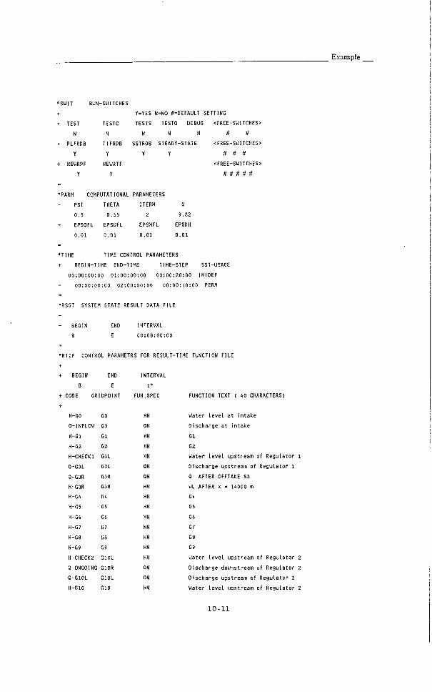
TEST
H
PLFRDB
Y
NEWRPF
Y
RUN-SWITCHES
TESTC
N
TIFRDB
Y
NEWRTF
Y
Y-YES N-HO ^-DEFAULT SETTING
TESTS TESTO DEBUG <FREE-SWITCHES>
H H N tl H
SSTRDB STEADY-STATE <FREE-SWITCHES>
Y Y H It tt
<FREE-SWITCHES>
II tl tl tt It
•PARH COMPUTATIONAL PARAMETERS
+ PSI THETA ITERH G
0.5 0.55 2 9.82
+ EPSOFL EPSUFL EPSHFL EPSDH
0.01 0.01 0.01 0.01
*TIHE TIME CONTROL PARAMETERS
+ BEGIN-TIME END-TIME TIME-STEP SST-USAGE
00:00:00:00 01:00:00:00 00:00:20:00 INIDEF
00:00:00:00 02:00:00:00 00:00:10:00 PERM
•RSST SYSTEM STATE RESULT DATA FILE
+
t BEGIN END INTERVAL
B E 00:08:00:00
•RTIF CONTROL PARAMETRS FOR RESULT-TIME FUNCTION FILE
+ BEGIN END INTERVAL
B E I *
+ CODE GRIDPOINT FUN.SPEC FUNCTION TEXT ( 40 CHARACTERS)
H-GO
Q-INFLOW
H-Gl
H-G2
H-CHECKl
Q-G3L
0-G3R
H-G3R
H-G4
H-G5
H-G6
H-G7
H-G8
H-G9
H-CHECK2
Q-ONGOING
Q-GIOL
H-GIO
G O
GO
Gl
G2
G3L
G3L
G3R
G3R
04
G5
G6
G7
G8
G9
GIOL
GIOR
GIOL
GIO
HN
QN
HN
HN
HN
QN
QN
HN
HN
HN
HN
HN
HN
HN
HN
QH
QN
HN
Water l e v e l a t i n t a k e
D i s c h a r g e a t i n t a k e
G l
G2
Water l e v e l u p s t r e a m of R e g u l a t o r 1
D i s c h a r g e upstream o f R e g u l a t o r 1
Q AFTER OFFTAKE S3
WL AFTER X - 14000 m
G4
G5
G6
G7
G8
G9
Water l e v e l u p s t r e a m of R e g u l a t o r 2
D i s c h a r g e downstream of R e g u l a t o r 2
D i s c h a r g e u p s t r e a m of R e g u l a t o r 2
Water l e v e l u p s t r e a m o f R e g u l a t o r 2
10-11
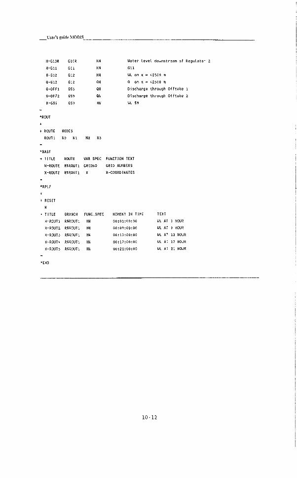
User's guide MODIS
H-GIOR
H-GU
H-G12
Q-G12
Q-OFFl
a-0FF2
H-GS9
GIOR
G U
G12
G12
GS3
GS9
GS9
HN
HN
HN
ON
QN
QN
HN
Water l e v e l downstream o f R e g u l a t o r 2
O i l
WL on X - «2500 m
Q on X • «2500 m
D i s c h a r g e t h r o u g h O f f t a l t e 1
D i s c h a r g e t h r o u g h O f f t a k e 2
WL S9
+ ROUTE NODES
ROUTl NO Nl N2 N3
"BASF
+ TITLE ROUTE VAR SPEC FUNCTION TEXT
N-ROUTE RSROUTl ORIDNO GRID NUMBERS
X-ROUTE RSROUTl X X-COORDINATES
+ RESET
N
+ TITLE BRANCH
H-ROUTl RJROUIl
H-R0UT2 RSROUTl
H-R0UT3 RSROUTl
H-ROUH RSROUTl
H-R0UT5 RSROUTl
FUNC.SPEC
HN
HN
HN
HN
HN
MOMENT IN TIME
00:01:00:00
00:09:00:00
00:13:00:00
00:17:00:00
00:21:00:00
TEXT
WL AT 1 HOUR
WL AT 9 HOUR
WL AT 13 HOUR
WL AT 17 HOUR
WL AT 21 HOUR
10-12
10.4 Result Data Base
The input data f i l e UTLIN.DAT of the subprogram RDBUTL i s shown below.
For more in f o r m a t i o n reference i s made to chapter 7.
Input file U T L I N . D A T
"FILS SPECIFICATION OF USED DATA SETS
INPUT UTLIN.DAT
ECHO UTLECH.OAT
OUTPUT UTLOUT.DAT
RDB-SST USSST.UNF
RDB-RTF USRTF.UNF
ROB-FILES IN GENERAL RESULT FUNCTION FORMAT
GR-FILEl USPLF.UNF
GR-FILE2 N
GR-F1LE3 N
GR-FlLEi, N
GR-F1LE5 USTIF.UNF
SELECT SWITCHES FOR UTL-ACTIONS
TRAFO-ACTION CONT-ACTION
Y Y
•TRAFO SPECIFICATION OF TIME RANGE FOR RESULT DATA BASE TRANSFORMATION
+ T-BEGIN T-END
B E
+
+ FUNCTIONS TO BE TRANSFORMED (OR ALFUN FOR ALL FUNCTIONS)
•CONT INVESTIGATE CONTENTS OF RESULT-OATABASE
+ TIME FUNCTIONS
+ SST RTF
'Y Y
+ PLACE-FUNCTIONS
t GRF-1 GRF-2 GRF-3 GRF-i, GRf-5
Y N N N Y
10-13

L'ser's guide MODIS
10.5 Model Results Tables
The r e s u l t s of the simulations can be presented i n various ways. Here the
input f i l e RESIN.DAT has been presented i n which each method of
presentation i s used. I n p r a c t i c e , not a l l of them are used
simultaneously.
I n p u t f i l e R E S I N . D A T
- ? R \ SPECIFICATION OF FILES ANO PAPER-FORMAT
+ USED DATA SETS
INPUT RESIN.DAT
ECHO RESECH.DAT
OUTPUT RESOUT.DAT
GR-FILEl USPLF.UNF
GR-FILE2 N
GR-FILE3 H
GR-FILE4 H
CR-FILE5 USTIF.UNF
+
+ CHARACTERS/LINE LINES/PAGE
132 60
+
+ SUMMARY OUTPUT ONLY (Y/H)
N
•BLK SPECIFICATION OF PRINT OUTPUT SET
+
+ BLOCK TITLE
Q O f f t a k e s & R e g u l a t o r s
+
+COLNO GR-FILE FORMAT UNITS FUNCTION FUNCTION FUNCTION FUNCTION
1 5 D:H:H:S TIME
2 # ...H3/S 0-INFLOU
3 It ...meter H-CHECKl
« It ..,H3/S 0-OFFl
5 H ...meter H-CHECK2
6 H ...H3/S H-GIOR
6 # ...H3/S 0-0FF2
7 # ...H3/S 0-ONGOING
10-14
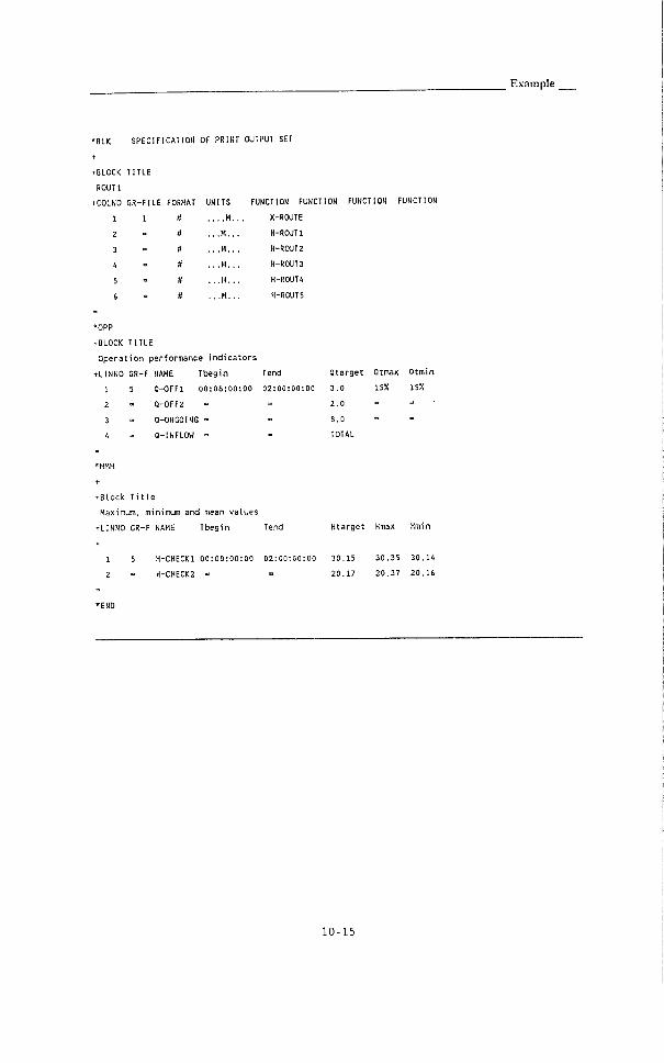
*BU SPECIFICATIOII OF PRINT OUTPUT SET
tBLOC< TITLE
ROUTl
+COLN0 GR-FILE FORMAT UNITS FUNCTION FUNCTION FUNCTION FUNCTION
1 1 11 H. . . X-ROUTE
2 ti . ..H,.. H-ROUTl
3 n ...H... H-R0UT2
1. tt ...H... H-R0UT3
5 tl ...H... H-R0UT4
6 ft ...H... H-R0UT5
•OPP
tBLOCK TITLE
O p e r a t i o n perfor^^ance i n d i c a t o r s
+LINNO GR-F NAHE T b e g i n Tend Q t a r g e t
1 5 Q-OFFl 00:08:00:00 02:00:00:00 3.0
2 - Q-0FF2 - - 2.0
3 - Q-ONGOING - - 8.0
4 - 0-INFLOU - - TOTAL
Qtmax
15%
Q t m i n
ISX
•rBlock T i t l e
M a x i m a , minimun and mean v a l u e s
•tLINNO GR-F NAME Tb e g i n Tend H t a r g e t Hmax
H-CHECKl 00:00:00:00 02:00:00:00
H-CHECK2 -
30.15
20.17
30.35 30.14
20.37 20.16
10-15

L'ser's guide MODIS
A f t e r running the subprogram MODRES, the output f i l e RESOUT.DAT w i l l look
as f o l l o w s .
Output file R E S O U T . D A T
05 APR 91 09:09:35 - 1-
TITLE : USED DATASETS
5 : 4 5
FUNCTION SUMMARY
COL NAHE FUNCTION DESCRIPTION TYP HIN.VALUE MAX.VALUE MEAN VAL. LEN
1 TIME TIME FUNCTION C ,00 .00 00 72
2 0-INFLOW D i s c h a r g e a t i n t a k e R 10, .00 13 ,00 12, 04 72
3 H-CHECKl Water t e v e l u p s t r e a m of R e g u l a t o r 1 R 30 , 13 30 , 19 30, 15 72
4 Q-OFFl D i s c h a r g e t h r o u g h O f f t a k e 1 R -, ,23 3 ,64 2, 97 72
5 H-CHECK2 Water l e v e l u p s t r e a m of R e g u l a t o r 2 R 20, ,09 20 ,25 20, 17 72
( Q-0FF2 D i s c h a r g e t h r o u g h O f f t a k e 2 R 1 , 57 4 ,37 2 .22 72
7 Q-ONGOING D i s c h a r g e downstream o f R e g u l a t o r 2 R ,00 7 .87 6 ,34 72
05 APR 91 09:09:35 - 2-
Q O f f t a k e s S R e g u l a t o r s
TIME Q-INFLOW H-CHECKl Q-OFFl H-CHECI<2 Q-0FF2 0-ONGOING
0:H:M:S ...H3/S ...meter ...H3/S ...meter ...H3/S ...H3/S
000 lOO ;20 ;00 10 .00 30, 14 -, ,23 20, 09 2. 15 ,01
000 ;00; ;40 :00 10 .00 30, 19 3, .64 20. 12 2. 25 ,00
000 ;01; ;00 ;00 10 ,00 30, 18 3 ,47 20, 09 1, 75 .77
000 ;01; ;20 ;oo 10 ,00 30. 13 2 ,63 20, 13 2, 40 .00
000 ;01; ;40 ;00 10 ,00 30, 16 3 ,15 20, 22 3, 80 .45
000 :02; ;00 ;00 10 .00 30, 14 2 ,86 20, ,25 4, 37 3.91
000 ;02; ;20 ;00 10 ,00 30, 14 2 .78 20, ,21 3, ,69 6.09
000; ;02; ;40 :oo 10 ,00 30, 16 3 , 19 20, 18 3, 15 5.87
000; ;03; ;00; :00 10 ,00 30, 14 2, ,81 20, 21 3, 70 5.41
000; ;03; ;20 ;00 10 .00 30. 15 3, ,00 20, 20 3, 43 6.45
000; ;03; ;40; ;00 10 ,00 30, 15 3 ,00 20, 18 3, 09 6.45
000; ;04; ;00; ;00 10, .00 30, 14 2 ,89 20, 20 3 ,52 6.22
000; ;04; 20; ;00 10 ,00 30, 15 3 ,04 20 17 3 ,07 6.82
000; ;04; 40; ;00 10, ,00 30, 15 2 ,95 20, ,16 3 ,24 6.50
10-16
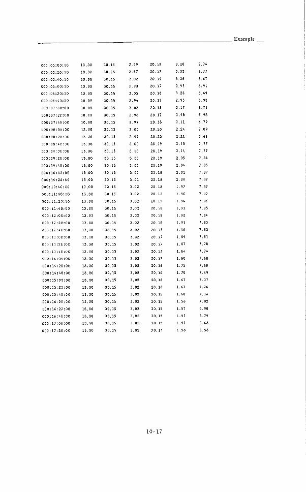
Example
000:05: 00: 00 10. 00 30. 15 2. 99 20.18 3. 20 6. 74
000:05: 20; 00 10. 00 30. 15 2. 97 20. 17 3. 03 6. 77
000:05: 40: 00 10. 00 30. 15 3. 02 20. 19 3, 26 6. 67
000:06: 0 0 : 00 10. 00 30. 15 2. 93 20. 17 2. 95 6. 91
000:06: 20: 00 10. 00 30. 15 3. 05 20. 18 3, 23 6. 69
000:06: 40:00 10. 00 30. 15 2. 94 20. 17 2. 95 6. 93
000:07: 00: 00 10.00 30. 15 3. 02 20. 18 3. 17 6. 75
000:07:20:00 10. 00 30. 15 2. 98 20. 17 2. 98 6. 92
000:07:40:00 10.00 30. 15 2. 99 20. 18 3. U 6. 79
000:08:00:00 13. 00 30. 15 3 . 00 20. 20 2. 24 7. 09
000:08:20:00 13. 00 30. 15 2. 99 20. 20 2. 21 7. 66
000:08: 40: 00 13. 00 30. 15 3, 00 20. 19 2. 10 7. 77
000:09: 00: 00 13. 00 30. 15 3, 00 20. 19 2. 11 7, 77
000:09: 20: 00 13. 00 30.15 3, 00 20. 19 2, 05 7, 84
000:09: 40:00 13. 00 30. 15 3, ,01 20. 19 2, 04 7, 85
0 0 0 :10; 00; 00 13, ,00 30, 15 3, .01 20. 18 2, ,01 7, ,87
000:10; ;20; ;00 13.00 30, , 15 3 ,01 20, 18 2, ,00 7 ,87
000:10; ;40; ;00 13 ,00 30, , 15 3 ,02 20, 18 1 ,97 7 ,87
000:11 ;00 :00 13 .00 30 , 15 3 ,02 20, , 18 1 ,96 7 ,87
0 0 0 :11 :20 :oo 13.00 30 ,15 3 .02 20, , 18 1 ,94 7 ,86
000:11:40 :00 13 .00 30 , 15 3 .02 20 , 18 1 .93 7 ,85
0 0 0 :12 :oo :0O 13.00 30 . 15 3 .02 20 , 18 1 .92 7 ,84
000:12 :20 : 00 13 .00 30 . 15 3 .02 20 , 18 1 .91 7 .83
000:12 :40 :00 13 .00 30 . 15 3 .02 20 ,17 1 .90 7 .82
0 0 0 :13 :00 :00 13 .00 30 . 15 3 .02 20 , 17 1 . 89 7 .81
0 0 0 ;13 :20 :oo 13 .00 30 . 15 3 .02 20 , 17 1 .87 7 .78
000:13 :40 :00 13 .00 30 , 15 3 .02 20 . 17 1 .84 7 .74
ooo: 14 :00 :00 13 .00 30 , 15 3 .02 20 , 17 1 .80 7 .68
000:14 :20 :00 13 .00 30 . 15 3 .02 20 .16 1 .75 7 .60
ooo:14:40 :oo 13 .00 30 .15 3 .02 20 . 16 1 .70 7 .49
000:15 :00 :00 13 .00 30 . 15 3 .02 20 .16 1 .67 7 .37
000:15 :20 :00 13 .00 30 .15 3 .02 20 , 16 1 .63 7 .26
000:15 ;40 :00 13 .00 30 .15 3 .02 20 , 15 1 .60 7 . 14
000:16 :oo :00 13 .00 30 .15 3 .02 20 . 15 1 .58 7 .02
000:16 :20:00 13 .00 30 .15 3 .02 20 . 15 1 .57 6 .90
ooo:16 :40 :oo 13 .00 30 .15 3 .02 20 . 15 1 .57 6 .79
000:17 :00 :oo 13 .00 30 . 15 3 .02 20 . 15 1 .57 6 .68
000:17 :20 :oo 13 .00 30 . 15 3 .02 20 .15 1 .58 6 . 58
10-17

L'ser's guide M0I)1S_
05 APR 91 09:09:35 - 3-
Q O f f t a k e s & R e g u l a t o r s
TIME O-INFLOW H-CHECICl 0-OFFl H-CHECK2 OH3FF2 Q-ONGOING
0:H:H:S ...H3/S ...meter ...H3/S ...meter ...H3/S ...H3/S
ooo: 17:40:00 13. 00 30. 15 3.02 20. 15 1. 59 6. 49
000:18:00:00 13. 00 30. 15 3.02 20. 15 1. 62 6. 42
000:18:20:00 13. 00 30. 15 3.02 20. U 1. 63 6 , 36
000:18:40:00 13. 00 30. 15 3.02 20. 16 1 , 64 6, 29
000:19:00:00 13. 00 30. 15 3.02 20. 16 1. 65 6, 21
ooo:19:20:00 13, ,00 30. 15 3.02 20. 16 1, 69 6 , 16
000:19:40:00 13, ,00 30. 15 3.02 20. 16 1, 71 6 , 14
000:20:00:00 13 ,00 30. 15 3.02 20. 16 1, ,72 6 , 12
000:20:20:00 13 ,00 30. 15 3.02 20. 16 1, ,72 6 ,09
000:20:40:00 13 ,00 30, , 15 3.02 20, 16 1 ,73 6 ,04
000:21:00:00 13 ,00 30 , 15 3.02 20, 16 1 ,76 6 ,00
000:21:20:00 13 .00 30 ,15 3.02 20, 16 1 ,76 6 ,00
000:21:40:00 13 .00 30 , 15 3.02 20, ,17 1 ,77 5 .98
000:22:00:00 13 .00 30 ,15 3.02 20, , 17 1 ,79 5 .96
000:22:20:00 13 .00 30 , 15 3.02 20, , 17 1 ,79 5 .99
000:22:40:00 13 .00 30 . 15 3.02 20 , 17 1 ,81 5 .97
000:23:00:00 13 .00 30 .15 3.02 20 ,17 1 .81 5 .99
000:23:20:00 13 .00 30 . 15 3.02 20 . 17 1 .81 5 .99
000:23:40:00 13 .00 30 . 15 3.02 20 , 17 1 .83 6 .00
001:00:00:00 13 .00 30 .15 3.02 20 .17 1 .83 6 .03
05 APR 91 09:09:36 - 4-
FUNCTION SUMMARY
USED DATASETS
TYP MIN.VALUE HAX.VALUE MEAN VAL. LEN
.00 42500.00 22553,83 60
8.40 31.98 26.33 60
8.40 32.30 26.25 60
8.40 32.69 26.21 60
6.40 32.93 26.18 60
8.40 33.10 26.19 60
FUNCTION DESCRIPTION
1 X-ROUTE
2 H-ROUTl
3 H-R0UT2
4 H-R0UT3
5 H-R0UT4
6 H-R0UT5
ATES
00:00
00:00
00:00
00:00
00:00
WL AT 1 HOUR
WL AT 9 HOUR
WL AT 13 HOUR
WL AT 17 HOUR
WL AT 21 HOUR
10-18
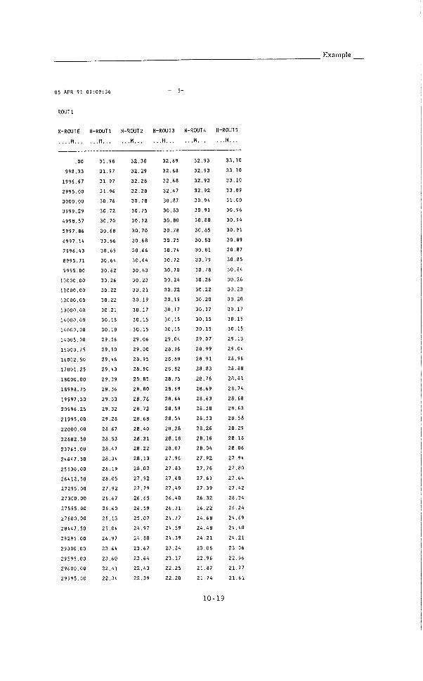
E x a m p l e
OS APR 91 09:09:36 - 5-
ROUTl
X-ROUTE H-ROUTl H-R0UT2 H-R0UT3 H-R0UT4 H-R0UT5
H . .H. . ..H... . .H. . . .H. .
00 3 1 . 98 32. 30 32.69 32. 93 33. 10
998. 33 3 1 . 97 32.29 32.68 32.93 33. 10
1996. 67 3 1 . 97 32.28 32.68 32. 93 33. 10
2995. 00 3 1 . 96 32.28 32.67 32. 92 33. 09
3000. 00 30. 76 30. 78 30.87 30. 94 3 1 . 00
3999. 29 30. 72 30. 75 30.83 30. 91 30. 96
4998. 57 30. 70 30. 72 30.80 30. 88 30. 94
5997. 86 30.68 30. 70 30.78 30. 85 30. 91
6997. 14 30. 66 30. 68 30.75 30. 83 30. 89
7996.43 30. 65 30. 66 30.74 30. 81 30. 87
8995. 71 30. 64 30. 64 30.72 30. 79 30. 85
9995, 00 30, 62 30. 63 30.70 30. 78 30, 84
10000, ,00 30, 26 30. 23 30.24 30. 26 30. 26
11000.00 30 ,22 30. 21 30.22 30, 22 30, 23
12000 ,00 30 ,22 30, 19 30.19 30, ,20 30, ,20
13000 ,00 30 ,21 30. 17 30.17 30, , 17 30 , 17
14000 ,00 30 , 18 30, , 15 30.15 30.15 30 , 15
14000 ,00 30 .18 30 .15 30.15 30 , 15 30 , 15
14005 ,00 29 .56 29 .06 29.04 29 ,07 29 ,13
15003 .75 29 .50 29 .00 28.96 28 .99 29 .04
16002 .50 29 .46 28 .95 28.89 28 .91 26 .96
17001 .25 29 .43 28 .90 28.82 28 .83 28 .88
18000 .00 29 .39 28 .85 28.75 28 .76 28 .81
18998 .75 29 .36 28 .80 28.69 28.69 28 .74
19997 .50 29 .33 28 .76 28.64 28.63 28 .68
20996 .25 29 ,32 28 .72 28.59 28 .58 28 .63
21995 .00 29 ,28 28 .68 28.54 28 .53 28 .58
22000 .00 28 .67 28 .40 28.28 28 .26 28 .29
22882 . 50 28 .53 28 .31 28.18 28 . 16 28 . 18
23765 .00 28.47 26 .22 28.07 28 .04 28 .06
24647 .50 28 .34 28.13 27.96 27 .92 27 .94
25530 .00 28 . 19 28 .02 27,83 27 .78 27 .80
26412.50 28 .05 27 .92 27,68 27 .61 27 .64
27295 .00 27 .92 27 .79 27,49 27 .39 27 .42
27300 .00 26.67 26 .65 26.40 26 .32 26 .34
27595 .00 26 .60 26 . 59 26.31 26 .22 26 .24
27600 .00 25 . 13 25 .07 24.77 24 .68 24 .69
28447 .50 25 ,04 24 .97 24 .59 24 .48 24 .48
29295 .00 24 ,97 24 .88 24 .39 24 .21 24 .21
29300 .00 23 ,64 23 .67 23.24 23 .06 23 .06
29595 .00 23 ,60 23 .64 23.17 22 .96 22 ,96
29600 .00 22 .41 22 .43 22.25 21 .87 21 ,77
29995 .00 22 .34 22 .39 22,20 21 .74 21 ,61
10- 19
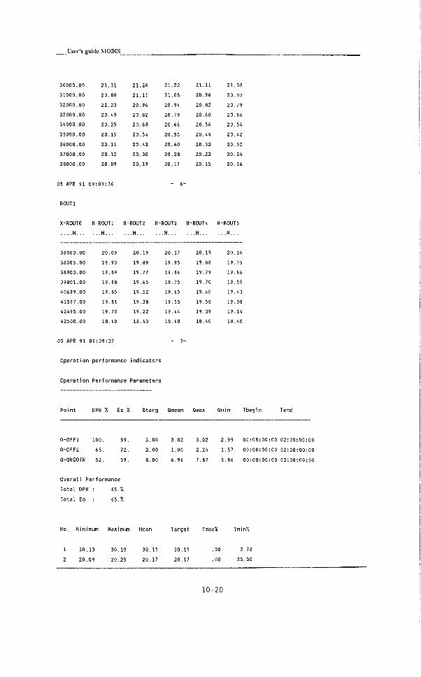
User's guide MODIS
30000. 00 21.31 21 , ,26 21.22 2 1 . 11 21.08
31000. 00 20.88 21, .11 21.08 20. 96 20.93
32000. 00 21.03 20, ,96 20.94 20. 82 20.79
33000. 00 20.49 20 ,82 20.79 20. 68 20.66
34000. 00 20.25 20, ,68 20.66 20. 56 20.54
35000. 00 20.15 20, ,54 20.53 20. 44 20.42
36000. 00 20.11 20, ,42 20.40 20. 33 20.32
37000, 00 20.12 20, .30 20.28 20. 23 20.24
38000, 00 20.09 20, ,19 20.17 20. 15 20. 16
05 APR 91 09:09:36 - 6-
ROUTl
X-ROUTE H-ROUTl H-R0UT2 H-R0UT3 H--ROUT 4 H-R0UT5
H . . .H .H. .H , .H. . ...H...
38000 .00 20.09 20 , 19 20.17 20. 15 20.16
38005.00 19.90 19 ,89 19.95 19. 88 19.75
38903 .00 19,89 19 ,77 19.86 19. 79 19.66
39801 .00 19,88 19 ,65 19.75 19. 70 19.55
40699 .00 19.85 19 ,52 19.65 19. 60 19.43
41597 .00 19.81 19 .38 19.55 19. 50 19.30
42495 .00 19.75 19 .22 19.44 19. 39 19. 14
42500 .00 18.40 18 .40 18.40 18. 40 18.40
05 APR 91 09:09:37 - 7-
O p e r a t i o n p e r f o r m a n c e i n d i c a t o r s
O p e r a t i o n Performance Parameters
P o i n t DPR % Eo !< O t a r g Qmean Qmax Qmin
Q-OFFl 100. 99. 3.00 3.02 3 ,02 2 ,99 00:08: iOO; ;00 02:00:00; ;00
Q-0FF2 65. 72. 2.00 1.80 2 ,24 1 ,57 00:08; ;00; ;00 02:00:00; ;00
Q-ONGOIN 52. 59. 8.00 6.96 7, ,87 5 ,96 00:08; ;00; :00 02:00:00; ;00
O v e r a l l P erformance
T o t a l DPR : 65.x
T o t a l Eo : 65.%
No. Minimum Maximun Mean T a r g e t Tmax% TminX
1 30.13 30.19 30.15 30.15 .00 2,73
2 20.09 20.25 20. 17 20.17 .00 25,00
10-20

E x a m p l e
10.6 Model results, Plots
The input f i l e PLTIN.DAT of subprogram MODPLT has been depicted below.
Both l o n g i t u d i n a l sections can be p l o t t e d , and, a f t e r removing the "-"
characters i n the f i r s t column, water l e v e l and discharge v a r i a t i o n as
a f u n c t i o n of time can be p l o t t e d .
Input file P L T I N . D A T
•PLOT - SPECIFICATION OF FILES AHD PAPER-FORMAT
+ USED DATASETS
INPUT PLTIN.DAT
ECHO PLTECH.OAT
OUTPUT PLTOUT.DAT
GR-FILEl USPLF.UNF
GR-FILE2 N
GR-FILE3 N
GR-FILE4 N
GR-FILE5 USTIF.UNF
+
1-PLOTTER DEVICE
VGA
- CGA
+
+TEXT FONT
- DRAFT
FINAL
•SIZE - PLOT SIZE
+
+ PLOT SIZE WIDTH HEIGHT
A3 # #
10-21

User's guide MODIS
•TEXT - PLOT TEXT
+
+ HEIGTH XCO YCO TEXT
+
il POSl H 0 D I S
II P0S2 New O e l f t I r r i g a t i o n
a P0S3 CANAL PERFORMANCE
# POS« D i s c h a r g e
0.4 P0S5 C i v i l E n g i n e e r i n g Dept
0.2 P0S6 T.U. DELFT
H P0S7
II P0S8
U P0S9
li POSIO
•AXES - SPECIFICATION OF AXES
+ AXIS NR 1 IS THE X-AXIS
NR. START END LEN GRD PLACE TEXT
1 00: :00:00:00 01:00:00:00 U N - T ime
1 0, ,0 42500 H N - D i s t a n c e
2 0, .0 13,1 It N L D i s c h a r g e
3 18, ,0 33,0 It N R Water l e v e l
•LINS - SPECIFICATION OF LINES IN DRAWING
+
+ NUMBER GR CODE UNIT FUNCTIONS (HAX. 5)
+ AXIS FILE
1 5 XX D:H:H:Y TIME
1 1 XX ..M.... X-ROUTE
3 - $1 ..H.... H-ROUTl
3 - SI . .H H-R0UT2
2 5 Si ..H3/S. 0-OFFl
2 - $2 ..H3/S. Q-0FF2
2 - 13 ..H3/S. 0-ONGOING
2 14 ..H3/S. 0-INFLOW
3 15 ..H... H-CHECK2
•END OF PLTDEF
10-22

E x a m p l e
10.7 Concluding remarks
The input f i l e s presented i n t h i s chapter can also be found on a d i s k e t t e
l a b e l l e d "DEMO.MOD". A f t e r a back up of t h i s d i s k e t t e has been made, one
can play w i t h the model, and see how the system reacts on v a r i a t i o n s i n
operation s t r a t e g y , gain f a c t o r s of the automatic upstream c o n t r o l l e r s ,
and/or other types of o f f t a k e s t r u c t u r e s .
10-23

L'ser's guide MODIS

11 Mathematical background
11.1 Canal flow
11.1.1 de Sa in t Venan t equations
I n MODIS program package, the unsteady flov; i n open c a n a l systems i s
computed on the b a s i s of two p a r t i a l d i f f e r e n t i a l equations of f i r s t
order. These "de S a i n t Venant equations" read:
. ± ( b 9 1 ) . gA^ . g " ' Q t ? L 0 11.2
TE dx^^ A' ^ ol- AR'''^
With:
A - c r o s s s e c t i o n a l a r e a m
Q - di s c h a r g e m^/s
R = h y d r a u l i c radius m
b, = c r o s s s e c t i o n a l storage width m
h = water l e v e l m
n - Mannings r e s i s t a n c e c o e f f i c i e n t s/m^'^
- l a t e r a l inflow m^/s q
fl - Boussinesq c o e f f i c i e n t
a c c e l e r a t i o n due to g r a v i t y m/s^ g
X - d i s t a n c e a l o n g c a n a l a x i s m
t - time • s
Equation (11.1) r e p r e s e n t s c o n t i n u i t y of volume which equals c o n t i n u i t y
of mass when the d e n s i t y of water i s assumed to be co n s t a n t ( f l u i d i s
w e l l mixed). The second equation (11.2) r e p r e s e n t s c o n t i n u i t y of
momentum, which can be i n t e r p r e t e d as dynamic e q u i l i b r i u m of f o r c e s
i n c l u d i n g a c c e l e r a t i o n f o r c e s .
11-1
User's guide MODIS
11.1.2 A s s u m p t i o n s u n d e r l y i n g the de saint venant equat ions
The assumptions u n d e r l y i n g the De Saint Venant Equations can be found by
rev i e w i n g the d e r i v a t i o n of the equations. I based on the law of mass and
momentum c o n s e r v a t i o n , i s presented. The main s i m p l i f i c a t i o n s u n d e r l y i n g
the De S a i n t Venant Equations are l i s t e d :
1 ) The v e l o c i t i e s p e r p e n d i c u l a r to the d i r e c t i o n of flow are n e g l i g i b l e
(and thus the a c c e l e r a t i o n s a l s o ) as compared to the v e l o c i t y i n the
d i r e c t i o n of flow. T h i s i m p l i e s that the slope of the water l e v e l
p e r p e n d i c u l a r to the d i r e c t i o n of flow i s assumed to be h o r i z o n t a l .
2) A n e g l i g i b l e c u r v a t u r e of the water s u r f a c e i m p l i e s a h y d r o s t a t i c
p r e s s u r e d i s t r i b u t i o n perpendicular to the flow d i r e c c i o n (or bed
sl o p e ) .
3) F r i c t i o n l o s s e s i n unsteady flow are not s i g n i f i c a n t l y d i f f e r e n t
from those i n steady flow and therefore the same r e s i s t a n c e formulae
may be a p p l i e d .
4) D e n s i t y of the f l u i d i s assumed to be constant.
5) The d e r i v a t i v e s of the c o e f f i c i e n t of Boussinesq B, e x p r e s s i n g the
non-uniformity of the v e l o c i t y d i s t r i b u t i o n a c r o s s the wetted area,
are assumed to be constant.
6) The bed s l o p e s i s assumed to be s m a l l . So t h a t c o s ( s ) - 1 and
s i n ( s ) - s
7) L a t e r a l i n f l o w i s assumed to be perpendicular to the c a n a l a x i s and
t h e r e f o r e not c o n t r i b u t i n g to the momentum equation
8) Wind f o r c e s a re not incorporated. To i n c o r p o r a t e wind f o r c e s the
term b.w^ . 7.(p - <fi) should be added to the l e f t hand s i d e of equation
( 1 1 . 2 ) . (w •= wind v e l o c i t y , b - cross - s e c t i o n a l flow width, 7 - wind
c o n v e r s i o n c o e f f i c i e n t , p - wind d i r e c t i o n i n degrees, (p - d i r e c t i o n
of c a n a l a x i s i n degrees, measured clockwise from the north.
11-2
M a t h e m a t i c a l B a c k g r o u n d
1 1 . 2 Structures
11.2.1 Introduction
A vast; number of standard s t r u c t u r e s a re included i n MODIS, each w i t h i t s
own c h a r a c t e r i s t i c s t a g e - d i s c h a r g e curve. The stage d i s c h a r g e curve of
a s t r u c t u r e s p e c i f i e s the d i s c h a r g e through a s t r u c t u r e as a f u n c t i o n of
the upstream and downstream water l e v e l s . I t i s more c o r r e c t to use the
energy l e v e l s i n s t e a d of the water l e v e l s but, the d i f f e r e n c e between the
energy head and water l e v e l head i s u s u a l l y small as a r e s u l t of the low
v e l o c i t i e s i n c a n a l s . Besides water l e v e l s are more easy to measure. As
a r e s u l t water l e v e l s are used and a c o r r e c t i o n c o e f f i c i e n t i s i n t r o d u c e d
to c o r r e c t the ( s m a l l ) e r r o r of not t a k i n g the energy l e v e l s .
The l o c a t i o n of the water l e v e l s are important for the stage d i s c h a r g e
c u r v e s , as the water l e v e l s v a r y e s p e c i a l l y i n the neighbourhood of
s t r u c t u r e . This l o c a l v a r i a t i o n c l o s e to the s t r u c t u r e s i s a r e s u l t of
che a c c e l e r a t i o n and r e t a r d a t i o n of the flow.
I n MODIS computer package, the water l e v e l s are taken a t some d i s t a n c e
from the s t r u c t u r e , although the computational g r i d p o i n t s might be
l o c a t e d c l o s e to the s t r u c t u r e .
11-3
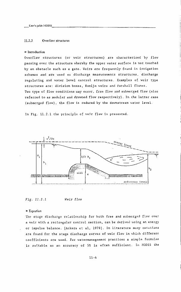
L'ser's guide M O D I S
11.2.2 O v e r n o w s t ruc tu res
• I n t r o d u c t i o n
Overflow s t r u c t u r e s ( o r weir s t r u c t u r e s ) are c h a r a c t e r i z e d by flow
p a s s i n g over the s t r u c t u r e whereby the upper water s u r f a c e i s not touched
by an o b s t a c l e such as a gate. Weirs a re f r e q u e n t l y found i n i r r i g a t i o n
schemes and are used as di s c h a r g e measurements s t r u c t u r e s , discharge
r e g u l a t i n g and water l e v e l c o n t r o l s t r u c t u r e s . Examples of weir type
s t r u c t u r e s a r e: d i v i s i o n boxes, Romijn w e i r s and P a r s h a l l flumes.
Two type of flow c o n d i t i o n s may occur, f r e e flow and submerged flow ( a l s o
r e f e r r e d to as modular and drowned flow r e s p e c t i v e l y ) . I n the l a t t e r case
(submerged f l o w ) , the flow i s reduced by the downstream water l e v e l .
I n F i g . 11.2.1 the p r i n c i p l e of weir flow i s presented.
r e f e r e n c e l e v e l
Fig. 11.2.1 Weir flow
" E q u a t i o n
The stage d i s c h a r g e r e l a t i o n s h i p f o r both f r e e and submerged flow over
a weir w i t h a r e c t a n g u l a r c o n t r o l s e c t i o n , can be d e r i v e d u s i n g an energy
or impulse b a l a n c e . [Ackers e t a l , 1978]. I n l i t e r a t u r e many notations
are found f o r the stage d i s c h a r g e curves of weir flow i n which d i f f e r e n t
c o e f f i c i e n t s are used. For watermanagement p r a c t i c e s a simple formulae
i s s u i t a b l e as an accuracy of 5% i s o f t e n s u f f i c i e n t . I n MODIS the
11-4

M a l h e m a t i c a l B a c k g r o u n d
n o t a t i o n a p p l i e d by Bos [Bos, 1976] i s used as t h i s n o t a t i o n i s g e n e r a l l y
accepted and f r e q u e n t l y used i n i r r i g a t i o n p r a c t i c e s .
The stage d i s c h a r g e r e l a t i o n s h i p reads:
c, - e f f e c t i v e d i s c h a r g e c o e f f i c i e n t
f - drowned flow r e d u c t i o n f a c t o r
h - upstream water l e v e l head m
b - width of the weir ™
z - c r e s t l e v e l of weir ™
u - exponent, normally 1.5
g _ a c c e l e r a t i o n due to g r a v i t y ni/s^
I n Equation (11-3) the upstream water l e v e l h i s used i n s t e a d of the
energy l e v e l head H. The e r r o r i n t r o d u c e d by n e g l e c t i n g the v e l o c i t y head
i n the approach c a n a l , i s c o r r e c t e d by the f a c t o r c„ which i n turn i s
i n c o r p o r a t e d i n the o v e r a l l c o r r e c t i o n f a c t o r c,. I n the.above n o t a t i o n
only d i m e n s i o n l e s s c o e f f i c i e n t s have been used.
The C g - c o e f f i c i e n t and the f a c t o r f are g e n e r a l l y determined e m p i r i c a l l y
and depend on f a c t o r s such as: the r a t e of submergence, the shape of the
s i l l c r e s t and the r a t i o h/d, where h i s the upstream head and d i s the
length of the s i l l c r e s t i n the d i r e c t i o n of flow.
The v a l u e of the power c o e f f i c i e n t u depends on the shape of the c o n t r o l
s e c t i o n . For r e c t a n g u l a r c o n t r o l s e c t i o n s u i s about 1.5 w h i l e f o r
t r i a n g u l a r c o n t r o l s e c t i o n s u = 2.5.
• Func t ions
The Cj and f c o e f f i c i e n t s can be given as a ( t a b u l a t e d ) f u n c t i o n . For
example, the c o r r e c t i o n c o e f f i c i e n t c^ can be g i v e n as a f u n c t i o n of the
upstream water l e v e l head and the drowned flow r e d u c t i o n f a c t o r f can be
given as a f u n c t i o n of ( h 2 - z ) / ( h l - z ) . ( F i g . 11.2.2).
11 .3
Where,
Q - d i s c h a r g e raVs
11-5
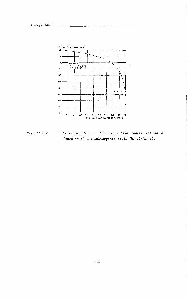
User's guide MODIS^
SUBV£KG£NCE RATO Hj /H ,
I i
1
. V. J.vd. CCRD IQJl
•
Hj/H, : ' / ! I
1 1
! i !
11.2.2 Value of drowned flow reducdon factor (f) as
function of the submergence ratio (h2-z)/(hl-z) .
11-6

M a t h e m a t i c a l B a c k g r o u n d
11.2.3 Orillce Structures
• Introduction
O r i f i c e flow i s c h a r a c t e r i z e d by flow p a s s i n g under gates whereby the
upper water s u r f a c e touches the gate and r e s i s t a n c e i s n e g l i g i b l e .
O r i f i c e s t r u c t u r e s are f r e q u e n t l y found i n i r r i g a t i o n schemes and are
used as d i s c h a r g e r e g u l a t i n g and measurements s t r u c t u r e s and as water
l e v e l c o n t r o l s t r u c t u r e s .
The flow through an o r i f i c e can be e i t h e r f r e e or submerged (modular or
drowned). I n the l a t t e r case (submerged flow) the downstream water l e v e l
e f f e c t s the d i s c h a r g e through the o r i f i c e opening and the v e l o c i t y i s
l e s s than the c r i t i c a l v e l o c i t y . I n F i g . 11.2.3 The c h a r a c t e r i s t i c of
o r i f i c e flow i s depicted.
r e f e r e n c e l e v e l
Fig. 11.2.3 Orifice flow
• E q u a t i o n s
The e q u a t i o n f o r both free and submerged o r i f i c e flow with a r e c t a n g u l a r
c o n t r o l s e c t i o n reads:
. 11.4 Q - c^iibyjlgkh
11-7
L'ser's % luide M O D I S
Where,
Q _ discharge mVs
c, - e f f e c t i v e d i s c h a r g e c o e f f i c i e n t -
opening c o n t r a c t i o n c o e f f i c i e n t (0.63) -
b width of c o n t r o l s e c t i o n m
y opening h e i g h t of gate m
dh - head d i f f e r e n c e . m
g a c c e l e r a t i o n of g r a v i t y m/s^
I f the downstream water l e v e l does not e f f e c t the d i s c h a r g e (modular
flow) the head d i f f e r e n c e (dh) becomes:
i h - h 1 - (z^ fiy) . 5
Where,
z - s i l l l e v e l m
fi opening c o n t r a c t i o n c o e f f i c i e n t -
y gate opening height. m
I f the flow i s submerged, the head d i f f e r e n c e (dh) i s equal to
i h - h 1 - ^2 .6
Where h^ and hz are the upstream and downstream water l e v e l s r e s p e c t i v e l y .
• Free and submerged flow
The boundary between f r e e and submerged o r i f i c e flow can i n some c a s e s
be determined t h e o r e t i c a l l y but i s u s u a l l y determined e m p i r i c a l l y . T h i s
boundary i s a f u n c t i o n of the c o n t r a c t i o n c o e f f i c i e n t fi and the r a t i o ' s
( h i - z ) / y and ( h 2 - z ) / y .
I n the computer model MODIS, a f a c t o r f i s introduced to check which flow
c o n d i t i o n i s a p p l i c a b l e f o r a given upstream and downstream water l e v e l
and gate opening hei g h t . The model computes at every time step the a c t u a l
v a l u e of y / ( h 2 - z ) .
When the a c t u a l value of y / ( h 2 - z ) i s lower than the s p e c i f i e d v a l u e of f,
the flow i s assumed to be submerged. When the flow i s always f r e e f
11-8

M a l h e m a t i c a l B a c k g r o u n d
should be taken equal to zero. When on the other hand the flow i s always
submerged f should be taken equal to u n i t y .
• W e i r f l o w
When the downstream water l e v e l i s below the gate opening height and the
upstream head becomes l e s s than 1.5 times the gate opening h e i g h t , the
s t r u c t u r e w i l l a c t as a weir with a c, c o e f f i c i e n t of 1.0. Submerged w e i r
flow i s assumed when the downstream head i s more than 2/3 of the upstream
head. I n a l l other c a s e s , f r e e weir flow i s assumed. The equation f o r
submerged w e i r flow reads:
Q - 5 ( h 2 - z ) y 2 g ( h i - h 2 )
• Func t i ons
The submerged f a c t o r f can be given as a f u n c t i o n of the r a t i o y / ( h i - z ) .
( F i g . 11.2.4). The e f f e c t i v e discharge c o e f f i c i e n t c, i s u s u a l l y taken as
a c o n s t a n t but can be s p e c i f i e d a l s o as a f u n c t i o n of the r a t i o y / ( h i - z ) .
The c o n t r a c t i o n c o e f f i c i e n t fi depends on the r a t i o of the gate opening
h e i g h t and the upstream water l e v e l head y / ( h i - z ) and can be s p e c i f i e d by
the u s e r e i t h e r as a constant or as a f u n c t i o n of (y/h^-z) (Table 11.2.1)
S U B M E R G E D FUOiV
M O D U L A R F L O W
t
I ^
1
y,e H,
1
HATIO n i y , / w
Fig. 11.2.4 Value of submerged factor f for orifice flow with a
contraction coefficient of 0.611. [Bos, 1976]
11-9
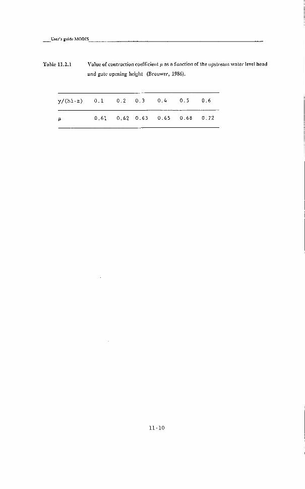
User's guide M O D I S
Table 11.2.1 Value of contraction coefficient ft as a function of the upstream water level head
and 1 jate opening height (Brouwer, 1986).
y / ( h l - z ) 0, ,1 0.2 0.3 0.4 0.5 0.6
M 0 .61 0.62 0.63 0.65 0.68 0.72
11-10

M a l h e m a t i c a l B a c k g r o u n d
11.2.4 P ipe
• I n t r o d u c t i o n
Pipe flow s t r u c t u r e s w i t h a v a r i a b l e c r o s s - s e c t i o n a l opening area are
standard i n c l u d e d i n MODIS. These s t r u c t u r e s a re i n p r i n c i p l e v e r y much
the same as the o r i f i c e flow s t r u c t u r e s . I n s t e a d of a gate opening height
and bottom width of c o n t r o l s e c t i o n , the wet c r o s s - s e c t i o n a l a r e a A i s
given. Example of t h i s type of o r i f i c e s t r u c t u r e s are gates w i t h a r a d i a l
gate opening and c u l v e r t s .
For pipe flow s t r u c t u r e s three flow c o n d i t i o n s are d i s t i n g u i s h e d ;
a e r a t e d f r e e flow, normal f r e e flow and submerged flow. The d i f f e r e n c e
between a e r a t e d and normal f r e e flow i s , t h a t i n the f i r s t case the
outgoing flow j e t i s f u l l y a e r a t e d w h i l e i n the second case (normal f r e e
flow) only the upper s u r f a c e of the outgoing flow i s a e r a t e d . As a r e s u l t
no h y d r o s t a t i c pressure can be assumed for f u l l y a e r a t e d flow, r e s u l t i n g
i n a somewhat d i f f e r e n t stage d i s c h a r g e curve.
The c h a r a c t e r i s t i c s of the three flow c o n d i t i o n s are pre s e n t e d i n F i g .
11.2.5 a, b and c.
• E q u a t i o n
The b a s i c equation for pipe flow reads:
Q . _ i _ A'JlgAh 11-8
Where,
Q - disc h a r g e mVs
- t o t a l l o s s c o e f f i c i e n t , c o n s i s t i n g of entrance, f r i c t i o n and
e x i t l o s s e s
A - c r o s s - s e c t i o n a l area of gate opening
dh = head d i f f e r e n c e .
^2
The head d i f f e r e n c e (dh) depends on the flow c o n d i t i o n . Three flow
c o n d i t i o n s are d i s t i n g u i s h e d :
11-11

a) free aerated flow
b) free flow
g|S__WOryy l e v e l
; i l i i i | i i . i i i . i i i : i i ;Mii ; , i : ; jw: i i l ; ; i : i i i l i iHi l i i i i i iuai i l i i laiiiiiiiuiiujiiiliBffiiiliaiiiiiiiiïisüiaiWllïïltllüil
r e f e r e n c e l e v e l
F i g . 11.2.5
c) submerged flow
Different flow conditions for pipe flow
11-12
M a l h e m a t i c a l B a c k g r o u n d
• A e r a t e d f l o w
I f the downstream water l e v e l i s below the bottom l e v e l of the opening,
the flow i s f u l l y a e r a t e d and dh becomes:
i h - hi - ( ^ t -'ibottom)
Where h^ i s the upstream water l e v e l , ht i s the top of opening and hbott=ro
i s the bottom l e v e l of the pipe.
B M o d u l a r How
I f the downstream water i s above the
the top of opening dh becomes:
i h - h^ - h.̂
bottom l e v e l of opening and below
11.10
• S u b m e r g e d f l o w
I f the downstream water l e v e l i s above the top l e v e l of opening, the flow
i s submerged and dh becomes:
Where i s the downstream water l e v e l .
• P a r t l y f i l l ed p ipe ( low
When the downstream water l e v e l i s below the top of opening of the pipe,
the pipe can be p a r t l y f i l l e d , depending on the upstream water l e v e l .
When the upstream water l e v e l i s above a c r i t i c a l l e v e l , the pipe i s
assumed to be completely f i l l e d . The c r i t i c a l l e v e l i s equal to :
''critical " bottom * (^T ~''bottom )
Whereby the f a c t o r f i s s p e c i f i e d by the user. Normally f v a r i e s between
1.5 and 1.2, the l a t t e r f o r longer pipe lengths.
I f the upstream water l e v e l i s below the c r i t i c a l l e v e l the pipe i s
p a r t l y f i l l e d and the weir flow equation i s a p p l i e d . The flow can be
e i t h e r f r e e or submerged depending on the r a t i o of the upstream and
downstream head. When the downstream head i s l e s s than 2/3 of the
upstream head, f r e e weir flow i s assumed:
11-13
L'ser's guide M O D I S
" t "bottom
I f the downstream head i s g r e a t e r than the upstream head, drowned weir
flow i s assumed:
Q-JT^ (''Z-''bottom) 11-1^ " t " "bottom
• T h e loss coef f ic ient
The l o s s c o e f f i c i e n t c, c o n s i s t of :
-entrance l o s s c o e f f i c i e n t :
c . ( 1 - 1 ) 2 11.15
^entrance V—
- r e s i s t a n c e l o s s c o e f f i c i e n t :
. 2 g i 11.16 '-resistance j ^ J ^ 4 / J
- e x i t l o s s c o e f f i c i e n t ( 1 . 0 ) :
11.17
Where, D - diameter of pipe, k - S t r i c k l e r r e s i s t a n c e c o e f f i c i e n t and L
- l e n g t h of pipe.
• Func t ions
The user can s p e c i f y the e f f e c t i v e d i s c h a r g e c o e f f i c i e n t c^ and the
c o n t r a c t i o n c o e f f i c i e n t n e i t h e r as c o n s t a n t s or as a f u n c t i o n e.g. of
the upstream water l e v e l . The p h y s i c a l p r o p e r t i e s of o r i f i c e s t r u c t u r e
the the s i l l l e v e l Z j , and the l e v e l of top of opening Z 2 must be
s p e c i f i e d as constants.
11-14
MalhematicalBackground
11.2.5 Headloss structures
I n c a n a l syst;ems a l l k i n d of head l o s s s t r u c t u r e s , such as b r i d g e s and
in v e r t e d syphons, are f r e q u e n t l y found. These s t r u c t u r e s c r e a t e head l o s s
due to the r e t a r d a t i o n of the a c c e l e r a t e d flow and p o s s i b l y due to the
r e s i s t a n c e of the flow p a s s i n g through these s t r u c t u r e s . I n MODIS these
types of s t r u c t u r e s can be modelled as head l o s s s t r u c t u r e s .
The head l o s s due to abrupt p r o f i l e changes can be computed u s i n g the
formulae:
i h ™ c ^1
11.18
Where Q i s the di s c h a r g e and A i s the ( c o n t r a c t e d ) wet c r o s s - s e c t i o n a l
area. The v e l o c i t y downstream V 2 i s assumed to be n e g l i g i b l e as compared
to the v e l o c i t y V i . The user MODIS can s p e c i f y the c o e f f i c i e n t c and the
wet c r o s s s e c t i o n a l area A e i t h e r as constants or as a f u n c t i o n of other
parameters.
I n a d d i t i o n to head as a r e s u l t of s t r u c t u r e s head l o s s might a l s o occur
as a r e s u l t of a sudden i n c r e a s e of the c r o s s - s e c t i o n a l area. I n that
case the head i s computed as:
11.19 , ^ ( V i - V 2 ) = tih - c „
Where,
dh - head l o s s "
c - l o s s c o e f f i c i e n t
V l - flow v e l o c i t y a t the vena c o n t r a c t a m/s
V 2 - flow v e l o c i t y downstream ni/s
The flow v e l o c i t y v^ i s the v e l o c i t y at the vena c o n t r a c t a and equal to
V l - Q/A. I f the term ( V 1 - V 2 ) becomes ne g a t i v e , the head l o s s i s s e t to
zero, as no head l o s s occur when the flow i s a c c e l e r a t i n g .
A
11 c o e f f i c i e n t s c and A can be given as co n s t a n t s but a l s o as a f u n c t i o n
of time or any other f u n c t i o n r e f e r e n c e parameter.
11-15

L'ser's guide M O D I S
11.2.6 Neyrtec distributors
• Introduction
The French company ALSTHOM has developed a l i n e of simple equipments f o r
automatic water l e v e l and di s c h a r g e c o n t r o l . E s p e c i a l l y the Neyrtec
(former N e y r p i c ) modules or b a f f l e d i s t r i b u t o r s are popular i n i r r i g a t i o n
p r a c t i c e s . These modules m a i n t a i n a n e a r l y constant d i s c h a r g e
i r r e s p e c t i v e of s u b s t a n t i a l upstream and downstream water l e v e l
f l u c t u a t i o n s w i t h i n a s p e c i f i c range. The stage discharge r e l a t i o n s h i p s
of a l l the Neyrtec modules have been in c o r p o r a t e d as standard s t r u c t u r e s
i n MODIS. The c h a r a c t e r i s t i c of a Neyrtec module i s given i n F i g .
11.2.6.
cnorrjY l e v e l
r n f o r e i i c u I r v n l
Fig. 11.2.6 Neyrtec distributor
• Equation
The stage d i s c h a r g e r e l a t i o n s h i p of the Neyrtec modules are u s u a l l y given
i n graphs and t a b l e s . I n the model MODIS, these t a b l e s are a l s o used. For
a c e r t a i n water l e v e l , the corresponding discharge i s c a l c u l a t e d by means
of i n t e r p o l a t i o n . When the water l e v e l drops below the s i l l , the
di s c h a r g e i s s e t to zero. When the water l e v e l exceeds the maximum
a l l o w a b l e water l e v e l , a maximum d i s c h a r g e i s s e t . I n r e a l i t y too high
water l e v e l s w i l l cause overtopping of the modules.
The u s e r has to s p e c i f y the s i l l l e v e l of the module and the le n g t h of
the module. I n s t e a d of u s i n g the r e a l l ength i t i s advised to use the
11-16

M a t h e m a l i c a l B a c k y r o u n d
e f f e c t i v e l ength of the modules. Example, a r e a l l e n g t h of 0.32 m (Type
:X1) has an e f f e c t i v e l e n g t h of 0.30 ra as the nominal d i s c h a r g e i s 0.30
ra * 100 1/s/m - 30 1/s.
I n Table 5.5.2 the d i f f e r e n t modules and t h e i r c a p a c i t i e s have been
l i s t e d . The Roman numbers (X, L e t c e t e r a ) i n d i c a t e the c a p a c i t y i n l i t r e
per second per decimeter length. The A r a b i c numbers (1 or 2) i n d i c a t e the
amount of B a f f l e s . With two b a f f l e s the a l l o w a b l e range of the water
l e v e l v a r i a t i o n i s h i g h e r .
• Func t i ons
Both s t r u c t u r e parameters of the n e y r t e c d i s t r i b u t o r s can be g i v e n e i t h e r
as a c o n s t a n t v a l u e s or as a f u n c t i o n of other v a r i a b l e s such as time.
By v a r y i n g the width of the d i s t r i b u t o r , opening and c l o s i n g of modules
can be simulated, (see next paragraph)
11-17
L'ser's guide M O D I S
11.3 Structure operation
11.3 .1 I n t r o d u c t i o n
To f a c i l i t a t e o p e r a t i o n of s t r u c t u r e s , some s t r u c t u r e parameters such as
opening h e i g h t , s i l l l e v e l and width of c o n t r o l s e c t i o n should be
v a r i a b l e during a s i m u l a t i o n run. I n model MODIS two types of o p e r a t i o n
are o f f e r e d ;
Operation as a f u n c t i o n of time.
Operation as a f u n c t i o n of a dependent v a r i a b l e such as the water
l e v e l .
The f i r s t one i s an open loop c o n t r o l system and the l a t t e r i s a c l o s e d
loop c o n t r o l system.
• O p e n loop con t ro l
I n an open loop c o n t r o l system the o p e r a t i o n i s predefined as a f u n c t i o n
of time and the a c t u a l s t a t e of the system i s not c o n s i d e r e d . With t h i s
f a c i l i t y time scheduled c o n t r o l can be simulated such as i n manual
c o n t r o l l e d systems.
• C losed loop con t ro l
I n a c l o s e d loop c o n t r o l system, c o n t r o l i s based on the a c t u a l s t a t e of
the system. T h i s i m p l i e s that the a c t u a l s t a t e of the system, f o r example
a water i s being read by the c o n t r o l l e r . The c o n t r o l l e r transforms the
input s i g n a l i n t o an output s i g n a l . The t r a n s f o r m a t i o n f u n c t i o n can be
a f i x e d r e l a t i o n s h i p between input and output s i g n a l . T h i s i s c a l l e d
simple c l o s e d loop c o n t r o l . The t r a n s f o r m a t i o n f u n c t i o n can a l s o be a
more compl i c a t e d f u n c t i o n such as a P I D - c o n t r o l l e r . I n t h a t case one
speaks of advanced c l o s e d loop c o n t r o l .
11.3.2 Open loop cont ro l
Open loop c o n t r o l of an i r r i g a t i o n system can be simulated by s p e c i f y i n g
the v a l u e of a s t r u c t u r e parameter as a f u n c t i o n of time. The model
11-18
M a t h e m a t i c a l B a c k g r o u n d
checks during s i m u l a t i o n f o r each new time l e v e l the value of che
s t r u c t u r e parameters and a d j u s t them.
11.3.3 Closed l oop c o n t r o l
B S imp le closed loop c o n t r o l
Simple c l o s e d loop c o n t r o l i s s i m u l a t e d by s p e c i f y i n g the va l u e of a
s t r u c t u r e parameter as a f u n c t i o n of a model v a r i a b l e . This can be a
t a b u l a t e d f u n c t i o n or a f o r t r a n d e f i n e d f u n c t i o n . Examples of model
v a r i a b l e s a r e upstream water l e v e l , upstream head, downstream head.
(Table 5.5.1)
• A d v a n c e d closed loop con t ro l
Two types of advanced c l o s e d loop c o n t r o l l e r s a re a t present implemented
i n MODIS. These a r e :
a so c a l l e d s t e p - c o n t r o l l e r and
a P I D - c o n t r o l l e r .
11.3.4 Step c o n t r o l l e r
I n the step c o n t r o l l e r the c o n t r o l v a r i a b l e (water l e v e l ) i s kept w i t h i n
a s p e c i f i e d a l l o w a b l e range of v a r i a t i o n . I n s i d e t h i s range no a c t i o n i s
taken. When the c o n t r o l v a r i a b l e (e.g. water l e v e l ) i s outside Chis range
Che s t r u c t u r e parameter (e.g. s i l l l e v e l ) i s a d j u s t e d . The r a t e of
adjustment i s c o n s t a n t and s p e c i f i e d by a v e l o c i t y .
The output s i g n a l of a step c o n t r o l l e r i s computed by:
11.20 - Uf̂ * V A C
11-19

User's guide M O D I S
where,
ut - output s i g n a l
zO - constant (parm2)
V - speed of gate movement
et - d e v i a t i o n from s e t - p o i n t (- h - t a r g e t l e v e l )
The s e t po i n t can be v a r i a b l e w i t h Q. I n BIVAL c o n t r o l the formula reads:
Vmax
Where D i s a constant and Qpivot i s the d i s c h a r g e i n the p i v o t p o i n t .
U.3.S FED control
The P r o p o r t i o n a l I n t e g r a l D i f f e r e n t i a l ( P I D ) - c o n t r o l l e r i s more advanced
c o n t r o l mechanism. The c o n t r o l mechanism c o n s i s t s of three p a r t s as i t s
name i n d i c a t e s . Each mechanism w i l l be e x p l a i n e d subsequently.
• Proportional control.
A simple c o n t r o l system i s p r o p o r t i o n a l c o n t r o l a l s o r e f e r r e d to as P-
c o n t r o l (more p r o p e r l y c a l l e d p r o p o r t i o n a l - p o s i t i o n e d c o n t r o l ) . Under
p r o p o r t i o n a l c o n t r o l , the water s u r f a c e v a r i e s from one end of the
p r o p o r t i o n a l band f o r no flow to the other edge of the band f o r maximum
flow. The p o s i t i o n of the r e g u l a t o r i s d e f i n e d by m u l t i p l y i n g the
d e v i a t i o n of the c o n t r o l v a r i a b l e by a g a i n f a c t o r Kp. T h i s i m p l i e s t h a t
the gate opening i s p r o p o r t i o n a l to the d e v i a t i o n of the water l e v e l from
the s e t - p o i n t . The user has to s p e c i f y t h i s g a i n f a c t o r (Kp). I n a d d i t i o n
the s e t point has to be def i n e d and the i n i t i a l gate p o s i t i o n .
The output s i g n a l i s computed by:
11-20

M a t h e m a t i c a l B a c k g r o u n d
Where,
- c o n t r o l l e r output ( s i g n a l f o r r e g u l a t o r )
et, - d e v i a t i o n from s e t p o i n t ( t a r g e t v a l u e - a c t u a l v a l u e )
Kp =• p r o p o r t i o n a l gain f a c t o r
P r o p o r t i o n a l c o n t r o l are commonly found by automatic h y d r a u l i c
r e g u l a t o r s . The gate opening i s p r o p o r t i o n a l to the d e v i a t i o n from the
s e t - p o i n t . The accuracy of a P - c o n t r o l l e r i s s m a l l as d e v i a t i o n s from the
s e t p o i n t can not be avoided. For every new water l e v e l a new e q u i l i b r i u m
p o s i t i o n i s s e t . A small p r o p o r t i o n a l g a i n f a c t o r makes the c o n t r o l l e r
slow, w h i l e a too high f a c t o r causes overcompensation of the r e g u l a t o r
l e a d i n g to i n s t a b i l i t i e s . P r o p o r t i o n a l c o n t r o l i s g e n e r a l l y unacceptable
f o r c o n t r o l l i n g g r a v i t y d e l i v e r i e s because the p r o p o r t i o n a l band r e q u i r e d
to a c h i e v e s t a b l e flow i s too l a r g e . (Zimbelman,1983)
• I n t e g r a l con t ro l l e r
Sometimes a more thoughtful c o n t r o l i s n e c e s s a r y , as i f the c o n t r o l l e r
has a s o r t of memory of d e v i a t i o n s i n the p a s t . The i n t e g r a l c o n t r o l l e r
bases i t s output s i g n a l not only on the present d e v i a t i o n , but a l s o on
the p r e v i o u s d e v i a t i o n s by taken the sum of a l l d e v i a t i o n s up to the
p r e s e n t time. I n t h i s way, e x t r a o r d i n a r y d e v i a t i o n s are damped, but, on
the o t h e r hand, ve r y small d e v i a t i o n s can be undervalued. For example,
i f the a c t u a l water l e v e l has been above the t a r g e t l e v e l f o r a
c o n s i d e r a b l e p e r i o d of time, the sum of d e v i a t i o n s i s l a r g e p o s i t i v e . I f
the t a r g e t l e v e l i s almost reached, the i n t e g r a l c o n t r o l l e d gate does not
s t a b i l i z e , but w i l l s t i l l c l o s e r e l a t i v e l y quick, because of the l a r g e
i n t e g r a l . I n t h i s case, to reach the t a r g e t l e v e l , the water l e v e l needs
to drop below the t a r g e t l e v e l to reduce the i n t e g r a l . T h i s process w i l l
always cause an o s c i l l a t i o n around the t a r g e t l e v e l . I f the K j - f a c t o r i s
not too l a r g e , the o s c i l l a t i o n can damp out. C h a r a c t e r i s t i c f o r the
i n t e g r a l c o n t r o l l e r i s that i t always f o r c e s the process back to i t s s e t -
p o i n t .
The output s i g n a l of the i n t e g r a l c o n t r o l l e r reads:
u ( t ) - Kr t e ( t ) ^ ^ ' ^ i-o
11-21
l'ser's guide M O D I S
Where i s the i n t e g r a l gain f a c t o r .
In HODIS, compacer package, the sum of the deviations is not altered if
the gate is in its maximum or minimum position in order to avoid too
large values of the sum, which will result in a too slow response of the
integral controller.
• D i f f e r e n t i a l c o n t r o l l e r
I n case of sudden v a r i a t i o n s the P l - c o n t r o l l e d process (a c o n t r o l l e r w i t h
a p r o p o r t i o n a l and a i n t e g r a l f a c t o r ) does not s a t i s f y . T h i s can be
e x p l a i n e d as f o l l o w s : i n the i d e a l s i t u a t i o n , the r e g u l a t o r would
immediately respond on the v a r i a t i o n . As s t a t e d before, only the
p r o p o r t i o n a l f a c t o r Kp gives an output s i g n a l based on the p r e s e n t
d e v i a t i o n . The i n t e g r a l f a c t o r Kj has the f e a t u r e of damping
e x t r a o r d i n a r y d e v i a t i o n s according to h i s t o r y , which i s now the case. The
Kp-factor should be r a t h e r l a r g e to be able to respond on the sudden
change. T h i s would a f f e c t the performance of the system over a longer
time, and i n s t a b i l i t y might occur. That i s why the Kp-factor cannot
chosen as l a r g e as needed at t h i s s p e c i f i c s i t u a t i o n .
There i s the need f o r a f a c t o r which comes out at the s p e c i f i c case of
a sudden l a r g e v a r i a t i o n , and which e f f e c t i s n e g l i g i b l e i n more s t a b l e
c i r c u m s t a n c e s . The d i f f e r e n t i a l c o n t r o l l e r s a t i s f i e s t h i s demand wi t h the
f o l l o w i n g output s i g n a l :
u ( t ) - K^-(eit)-e(t-l)) 1
The K D - f a c t o r i s only a p p l i e d i f the expected changes i n water l e v e l need
to be c o r r e c t e d v e r y q u i c k l y . However, i f the s i g n of the K^-factor i s
chosen opposite to the s i g n of the Kp-factor, i t s e r v e s as a r e t a r d a t i o n
of the gate movement. T h i s can be u s e f u l i f very l a r g e sudden d e v i a t i o n s
are not d e s i r e d to be followed immediately by a c o n s i d e r a b l e change of
the gate s e t t i n g .
• P I D - c o n t r o l l e r
The PID ( P r o p o r t i o n a l , I n t e g r a l , D i f f e r e n t i a l ) c o n t r o l l e r combines three
types of c o n t r o l techniques. I f the d e v i a t i o n on time t i s expressed by
e(t), the output s i g n a l i s computed as:
11-22

M a l h e m a t i c a l B a c k g r o u n d
u(t:) -Kp-e(c) i - ^ C i ' J ^ C e ) • (e ( t ) - e( C - 1 ) )
The d e t e r m i n a t i o n of the b e s t v a l u e s of the three parameters of the PID
c o n t r o l l e r i s a process on i t s e l f , which asks f o r a more s y s t e m a t i c a l
approach. To o b t a i n the b e s t v a l u e s , i t should p o s s i b l e to use a program
with c o n t r o l parameter adjustment r u l e s , i n which s i m p l i f i e d Barré de
Saint-Venant equations are used. I t i s a l s o p o s s i b l e to use some r u l e s
d e r i v e d by Z i e g l e r and Nichols (Cool e t a l 1985). ( F i g . 4.3.3). Since
such a program i s not y e t a v a i l a b l e , a d i f f e r e n t approach i s n e c e s s a r y
not to get l o s t i n too much t r i a l - a n d - e r r o r . A proper understanding of
the i n f l u e n c e of each separate f a c t o r i s needed to be able to g a i n good
v a l u e s .
The Kp-factor i s the p r o p o r t i o n a l f a c t o r . T h i s means that the measured
d e v i a t i o n i s p r o p o r t i o n a l l y compensated f o r . Most of the c a s e s , the Kp-
f a c t o r i s g r e a t e r than u n i t y , which means the gate w i l l open more than
the sensed d e v i a t i o n from the t a r g e t l e v e l . T h is f a c t o r p l a y s an
important p a r t i n the gate c o n t r o l , s i n c e i t g i v e s a r e a c t i o n to the gate
as soon as a d e v i a t i o n i s measured.
• S u m m a r i z e d :
Kp: fo r a immediate, p r o p o r t i o n a l d e v i a t i o n r e l a t e d change of the gate;
u s u a l l y the l a r g e s t f a c t o r . The t a r g e t l e v e l w i l l never be obtained,
but the water l e v e l o s c i l l a t e s around i t .
KJ: f o r a memory-based c o n t r o l of the gate, to damp out sudden
v a r i a t i o n s and thus obtain more s t a b i l i t y and a water l e v e l equal to
the t a r g e t l e v e l . T h i s f a c t o r i s commonly s m a l l .
KD: to have a quick response on sudden changes, or opposite a tamed
response on sudden changes, dependant on the s i g n of the f a c t o r . The
f a c t o r i s chosen r e l a t i v e to the expected changes, but normally
s m a l l e r than Kp.
An optimal c o n t r o l l e r has the f o l l o w i n g p r o p e r t i e s ;
- quick response
- s u f f i c i e n t damping to avoid i n s t a b i l i t i e s
- s m a l l s t a t i c d e v i a t i o n
11-23

User's guide M O D I S
I n f a c t these requirements are c o n t r a d i c t o r y . T h e r e f o r e , i t i s needed to
f i n d a compromise between the mention requirements.
Zieg ler N icho ls a d j u s t m e n t ru les
a l l f a c t o r s a re s e t to zero, except the Kp-factor. T h i s f a c t o r i s
chosen minimal, but so that a s t a b l e o s c i l l a t i o n i s j u s t acquired,
T h i s corresponds w i t h the graph below. The used Kp-factor i s c a l l e d
Ky, the u l t i m a t e g a i n .
the p e r i o d of the obtained o s c i l l a t i o n i s c a l l e d the u l t i m a t e period
Tu, and can be measured from the graph.
the v a l u e s of the gain
f a c t o r s can then be derived
as:
induced osciltal
0.S9-K,,
= 1.18. • At
Fig. 4.3.3 Ziegler-Nichols rules 0.074
AC
The v a l u e s thus obtained can serve as a f i r s t e s t i m a t i o n of the input for
the c o n t r o l l e r , and might need to be a d j u s t e d f o r the s p e c i f i c s i t u a t i o n .
11-24

MathematicalBackground
11.3.6 Local and regional control
I n g e n e r a l , t;hree l e v e l s of c o n t r o l a re d i s t i n g u i s h e d ; l o c a l , r e g i o n a l
and g l o b a l c o n t r o l . I n MODIS l o c a l and r e g i o n a l c o n t r o l have been
implemented. When a r e g u l a t o r i s l o c a l c o n t r o l l e d , c o n t r o l c o n s i s t of one
c o n t r o l loop, whereby the sensor i s p l a c e d i n the d i r e c t neighbourhood
of the r e g u l a t o r . Regional c o n t r o l i s an inte r m e d i a t e l e v e l between l o c a l
and g l o b a l c o n t r o l and i s a p p l i e d when measurements other than at the
r e g u l a t o r s i t e , are r e q u i r e d .
• Local
Standard l o c a l automatic c o n t r o l systems i n c l u d e d i n MODIS are upstream
c o n t r o l , downstream c o n t r o l and mixed c o n t r o l . Automatic water l e v e l
c o n t r o l i s only p o s s i b l e f o r the weir and o r i f i c e types of s t r u c t u r e s .
I n case of l o c a l upstream c o n t r o l , the water l e v e l i n the g r i d p o i n t j u s t
upstream of the r e g u l a t o r i s used as the input v a r i a b l e of the
c o n t r o l l e r . I n case of downstream c o n t r o l , the water l e v e l , downstream
of the r e g u l a t o r i s used. For mixed c o n t r o l both l e v e l s are used.
• Regional control
When r e g i o n a l c o n t r o l i s a p p l i e d two water l e v e l s e n s o r s can be pl a c e d
anywhere a t a user d e f i n e d g r i d - p o i n t . The input of the c o n t r o l l e r i s
weighed average of these two water l e v e l s . The weighing c o e f f i c i e n t s are
a f o r the f i r s t g r i d p o i n t and 1-a f o r the second g r i d p o i n t .
11-25
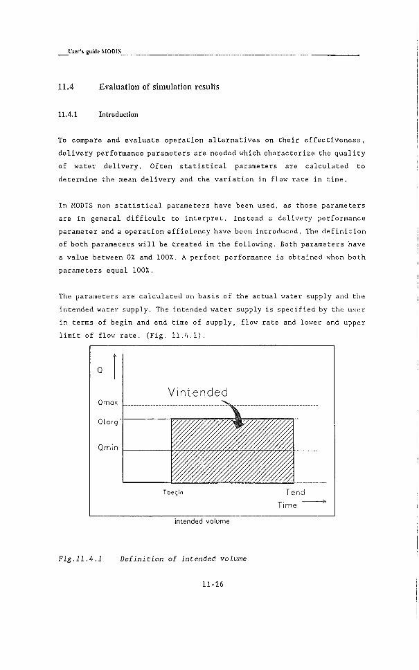
11.4 Evaluation of simulation results
11.4.1 I n t r o d u c t i o n
To compare and e v a l u a t e o p e r a t i o n a l t e r n a t i v e s on t h e i r e f f e c t i v e n e s s ,
d e l i v e r y performance parameters are needed which c h a r a c t e r i z e the q u a l i t y
of water d e l i v e r y . Often s t a t i s t i c a l parameters are c a l c u l a t e d to
determine the mean d e l i v e r y and the v a r i a t i o n i n flow r a t e i n time.
I n HODIS non s t a t i s t i c a l parameters have been used, as those parameters
are i n g e n e r a l d i f f i c u l t to i n t e r p r e t . I n s t e a d a d e l i v e r y performance
parameter and a o p e r a t i o n e f f i c i e n c y have been introduced. The d e f i n i t i o n
of both parameters w i l l be t r e a t e d i n the f o l l o w i n g . Both parameters have
a v a l u e between OX and 100%. A p e r f e c t performance i s obtained when both
parameters equal 100%.
The parameters are c a l c u l a t e d on b a s i s of the a c t u a l water supply and the
intended water supply. The intended water supply i s s p e c i f i e d by the u s e r
i n terms of begin and end time of supply, flow rate and lower and upper
l i m i t of flow r a t e . ( F i g . 11.4.1).
Q
V i n t e n c d e d Omox
Q t o r g
Qmin
T b e g i n T e n d
T ime
I n t e n d e d v o l u m e
Fig.11 A.l Definition of intended volume
11-26

M a t h e m a t i c a l B a c k g r o u n d
By d e f i n i n g the intended flow r a t e and dur a t i o n of supply, the t o t a l
intended volume to be su p p l i e d , h e r e a f t e r c a l l e d the intended volume
( V i ) , i s f i x e d . The lower and upper l i m i t of acceptable flow r a t e s a l l o w s
f o r some v a r i a t i o n i n flow r a t e s .
The a c t u a l s u p p l i e d volume r e c e i v e d by an o f f t a k e (Va) i s computed by
i n t e g r a t i n g the a c t u a l flow r a t e with r e s p e c t to the s p e c i f i e d time
i n t e r v a l . However, the a c t u a l flow r a t e r e c e i v e d by an o f f t a k e during the
s p e c i f i e d time i n t e r v a l might exceed the allowable range of flow r a t e s .
T h e r e f o r e , the a c t u a l flow r a t e i s considered to be an e f f e c t i v e flow
r a t e when the a c t u a l flow r a t e i s w i t h i n the s p e c i f i e d boundaries. When
the a c t u a l flow r a t e exceeds the upper boundary, the e f f e c t i v e flow r a t e
i s taken a t the upper boundary. A too high flow r a t e f o r example, might
l e a d to s p i l l a g e whereas a too sm a l l flow r a t e might not be handled a t
a l l .
The e f f e c t i v e s u p p l i e d volume (Ve) can now be c a l c u l a t e d by i n t e g r a t i n g
the e f f e c t i v e flow r a t e with r e s p e c t to the s p e c i f i e d time i n t e r v a l . When
the e f f e c t i v e s u p p l i e d volume exceeds the intended volume, the e f f e c t i v e
volume i s taken equal to the intended volume as the a d d i t i o n a l s u p p l i e d
volume can not be considered to be e f f e c t i v e , although the flow r a t e s are
w i t h i n the s p e c i f i e d boundaries. ( F i g . 11.4.2)
Tbegin T e n d
Time
e f f e c t i v e v o l u m e
Fig. 11.4.2 Definidon of effective volume
11-27

User's guide M O D I S
Now three volumes have been computed, the intended volume, the a c t u a l
volume and the e f f e c t i v e volume. With these three volumes two o p e r a t i o n
performance parameters are computed.
11.4.2 Delivery performance ratio
The d e l i v e r y performance r a t i o (DPR) s p e c i f i e s to what extent the o f f t a k e
has r e c e i v e d i t s intended supply. The DPR i s defined as Che r a t i o of the
e f f e c t i v e volmne (Ve) and the intended volume ( V i ) , i n formulae:
DPR - 100% .29
11.4.3 Operation efficiency
The second parameter i s the operation e f f i c i e n c y (e^,) which s p e c i f i e s
with which e f f i c i e n c y the i r r i g a t i o n water i s d i s t r i b u t e d . The o p e r a t i o n
e f f i c i e n c y i s defined as the r a t i o of the e f f e c t i v e s u p p l i e d volume and
the a c t u a l supplied volume, i n formulae
eo - ^ 100% .30
Where,
DPR - D e l i v e r y performance r a t i o
eg - Operation e f f i c i e n c y
Vj - Volume a c t u a l d e l i v e r e d
V, - Volume e f f e c t i v e l y d e l i v e r e d
Vi - Volume intended to be d e l i v e r e d
An operation e f f i c i e n c y of 0% indicates that a l l water supplied i s lose,
whereas an operacion e f f i c i e n c y of 100% indicaCes ChaC a l l wacer supplied
i s e f f e c t i v e l y supplied.
11-28

M a t h e m a t i c a l B a c k g r o u n d
11.4.4 Ove ra l l pe r fo rmance
The o v e r a l l D e l i v e r y Performance R a t i o i s c a l c u l a t e d by a weighed average
of the DPR of the i n d i v i d u a l o f f t a k e s and read s :
n-p n-p
E^e.n EOP'̂ .n V l . n npn _ n - l _ n - l 11 . 31 " ^ ' < o v , r . U ^
E ^ i . n E ^ i . n n - l n - l
Where DPR^ v o r a i i i s the o v e r a l l D e l i v e r y Performance R a t i o , V, „ i s the
e f f e c t i v e volume r e c e i v e d by o f f t a k e n (m^) , „ i s the intended volume
to be r e c e i v e d by o f f t a k e n (m^) , and p i s the number of o f f t a k e s
i n v o l v e d .
The o v e r a l l operation e f f i c i e n c y i n c o r p o r a t e s the o p e r a t i o n a l l o s s e s of
the i n d i v i d u a l o f f t a k e s , the l o s s e s due to f i l l i n g up the c a n a l to i t s
o p e r a t i o n a l l e v e l , and the leakage l o s s e s and or s p i l l l o s s e s i f these
occur. Xn formula i t reads,
n - p
E ' ^ e . n 11.32 n - l
^ 0 , o v e r a l l " Tj ^ a , i n t a k e
Where eo^overaH i s the o v e r a l l o p e r a t i o n e f f i c i e n c y , Vg^intako i s the a c t u a l
i n t a k e volume at the head of the main c a n a l (m^) , V, ,, i s the e f f e c t i v e
volume r e c e i v e d by o f f t a k e n (m^) , and p i s the nuraber of o f f t a k e s
involved.
The o v e r a l l d e l i v e r y performance r a t i o becomes equal to the o v e r a l l
o p e r a t i o n e f f i c i e n c y i f the sum of intended volumes i s equal to the
volume taken i n . I n t h a t case the o v e r a l l performance of the c a n a l system
can be c h a r a c t e r i z e d by one s i n g l e f i g u r e .
• I n t e r p r e t a t i o n o f parameters
An o p e r a t i o n e f f i c i e n c y of 100% does not i n d i c a t e t h a t the o f f t a k e
r e c e i v e d enough water. Therefore both parameters should be used i n
combination. I n chat way the parameters becomes d i a g n o s t i c parameters as
w e l l . When f o r example both parameters are l e s s than 100%, the water
11-29
User's guide M O D I S
manager knows t h a t there i s s t i l l room for improvements, without
i n c r e a s i n g the a c t u a l water supply.
• Genera l r e m a r k s
I n l i t e r a t u r e other performance parameters are found. Examples are the
Operation Performance R a t i o (OPR) d e f i n e d by [Lenton, 1982] and used by
[ I I M I , 1987], [Makin,1986] and [ F r a n c i s & Elawad,1989]. The Operation
performance R a t i o i s def i n e d as the r a t i o between the a c t u a l flow r a t e
and the intended flow r a t e . The drawbacks of the OPR i s that only the
flow r a t e i s c o n s i d e r e d and not the moment of d e l i v e r y . B esides, no
e x p l i c i t r e l a t i o n i s made with the i r r i g a t i o n e f f i c i e n c y .
11-30

12 Numerical solution
12.1 Introduction
The unsteady flow i n open canals i s described by the de Saint Venant
Equations. Both the equation of c o n t i n u i t y and the equation of momentum
of the de Saint Venant equations are p a r t i a l d i f f e r e n t i a l equations of
the f i r s t order. To solve t h i s set of two p a r t i a l d i f f e r e n t i a l equations,
the p a r t i a l d i f f e r e n t i a l s are replaced by f i n i t e d i f f e r e n c e equations
which can be solved numerically. I n MODIS the transformation from
d i f f e r e n t i a l s to f i n i t e d ifferences i s performed w i t h a four point
i m p l i c i t Preissmann scheme. (Cunge, Holly, Verwey, 1979)
I n Che transformed equations two unknowns can be d i s t i l l e d f o r every
computational g r i d p o i n t , namely AQ and Ah represencing the increment
during one time step At. The new values f o r Q and h at the new time l e v e l
become equal Co Che values at the previous time l e v e l plus the
increments.
Uhen a s t r u c t u r e i s located inside a branch, Che o r i g i n a l momentum
equation of th a t branch i s replaced by the stage discharge r e l a t i o n s h i p
of t h a t s t r u c t u r e . To do so, the stage discharge r e l a t i o n s h i p i s
r e w r i t t e n i n t o the same form as the o r i g i n a l momentum equation. I n t h i s
way che computation remains i m p l i c i t and no spe c i a l arrangements have to
be made i n the s o l u t i o n procedure.
I n t h i s chapter the d i s c r e t i z a t i o n of the canal flow equations, the
boundary conditions and Che sCrucCure equations w i l l be explained i n
d e t a i l . Furchermore Che soluCion procedure of Che unknowns i s CreaCed.
12-1

User's guide M0D1S_
12.2 Discretizing the canal flow equations
12.2.1 Genera l
For the s o l u t i o n of the system of flow equations, Verwey's v a r i a n t of the
Preissmann scheme has been chosen. (Cunge, Holy, Verwey, 1979). The
Preissraann scheme i s a four p o i n t i m p l i c i t scheme, which i m p l i e s t h a t
four v a r i a b l e s can be d i s t i n g u i s h e d namely AQ and Ah i n two a d j a c e n t g r i d
p o i n t s ( F i g . 12.2.1).
T l i a e
(n+1) i t
(n+O i t f
n i t
( j - l ) i X ( j - l + vS)iX j iX D i s t a n c e
Fig. 12.2.1 Preissmann scheme
The d e r i v a t i v e s with r e s p e c t to x and t are d i s c r e t i z e d on the g r i d shown
i n F i g . (12.2.1) as f o l l o w s :
eo , g / - g / - i
dx Ax
e ' A P , - A g , . , )
A x
12.1
Bh dt
Ah,-
Ac Ah. A t
12.2
12-2

N u m e r i c a l So lu t ion
Where,
AQj - QJ - QJ
n - s u p e r s c r i p t f o r time l e v e l
j - s u b s c r i p t f o r space l o c a t i o n
^ - a weighting c o e f f i c i e n t for d i s t r i b u t i n g the space d e r i v a t i v e s
over the two time l e v e l s nAt and (n+l)At and
a weighting c o e f f i c i e n t d e f i n e d s i m i l a r l y for d i s t r i b u t i n g
terms i n space.
12.2,2 C o n t i n u i t y equa t ion
The f u l l d i s c r e t i z e d form of the c o n t i n u i t y equation (Eq 10.1) now reads:
^ ^ ^ ^ L ^ ^ ( l - ^ ) 5 3 - ( f ^ . ̂ b ^ r ^ - 'iyl^l ^2.5
R e m a r k s
For the c o e f f i c i e n t b, the b e s t known approximation f o r i t s v a r i a t i o n
i n time w i l l be taken a t the p o i n t (n+4)At. E v a l u a t i n g the value of
the c o e f f i c i e n t s a t time l e v e l (n+1/2), i s the main p r i n c i p l e of
Verwey's v a r i a n t of the Preissmann scheme.
The l a t e r a l flow ( i n f l o w or outflow) i s s p e c i f i e d between two g r i d
p o i n t s and t h e r e f o r e w i l l be taken a t p o i n t (j-H)Ax, (n+H)At.
Equation (12.5) can be w r i t t e n i n a form l i k e :
/ i l j Ahj_i ^ B l j A Qj.i * C2j Ahj 4- Dl^ AQj - El^ 12.6
12-3
L'ser's guide M O D I S _
by m u l t i p l i c a t i o n of a l l terms by Ax. The ABCDE c o e f f i c i e n t s become:
il n h "-'/̂ Ax 12.7
C I , ^ 0 b , " - ^ ^ ^ 12.9
12.2.3 Momentum equation
The momentum equation (Eq 10.2) i s d i s c r e t i z e d f o l l o w i n g s i m i l a r
p r i n c i p l e s . I n the momentum equation however no n - l i n e a r terms appear
which have to be l i n e a r i z e d .
I n the o r i g i n a l model Rubicon, the co n v e c t i v e a c c e l e r a t i o n term i s
approximated i n an e x p l i c i t form. I n MODIS, an i m p l i c i t n o t a t i o n has been
used d i s t r i b u t e d over the g r i d point j - l and j .
The f r i c t i o n term i s d i s t r i b u t e d over Che g r i d points j - l and j w i t h
weighting c o e f f i c i e n t s of (1 - and V r e s p e c t i v e l y and the product
|Q|.Q i s w r i t t e n as a product of the di s c h a r g e at time l e v e l s nAt and
(n - l-l)At r e s p e c t i v e l y . I t can be proven that t h i s i s the most a c c u r a t e
schematizaCion of the r e s i s t a n c e term.
12-4

N u m e r i c a l S o l u t i o n
The f u l l f i n i t e d i f f e r e n c e scheme f o r the momentum equation i s then read;
A A
Ax
Ax Ax
12.12
M u l t i p l y i n g a l l terms by Ax, the c o e f f i c i e n t s i n the d i f f e r e n c e scheme
can be w r i t t e n i n the form:
A2j Ahj_i + B2j A Qj_i * C2, tih, * D2, AQj - E2,
Where the ABCDE c o e f f i c i e n t s read:
12.13
A2, - -n^X-\'l 12.14
B2 12.15
C2, - egAY-ljj n.\6
J AC 4̂ 12.17
A i j - i
12.18
12-5

L'ser's guide M O D I S ^
R e m a r k
For h i g h e r Froude numbers the c o n v e c t i v e a c c e l e r a t i o n term may le a d to
i n s t a b i l i t i e s . Under these c o n d i t i o n s i t i s b e t t e r to use a type of
d i f f u s i v e wave approximation. T h i s i s achieved by g i v i n g B-0 i n the
input, thus n e g l e c t i n g the con v e c t i v e a c c e l e r a t i o n term.
12-6

iN'umerici i l S o l u t i o n
12.3 Boundary conditions
For each c a n a l s e c t i o n ( t h a t i s a c a n a l e n c l o s e d between two
computational g r i d p o i n t s ) Equations (12.5) and (12.13) can be s e t up.
Suppose a branch i s d i s c r e t i z e d i n t o N g r i d p o i n t and i n every g r i d p o i n t
we d e f i n e two unknowns (namely AQ and Ah), then i n t o t a l there w i l l be
2N unknowns. However, there a re only ( N - l ) c a n a l s e c t i o n s and
consequently we can only d e f i n e 2 ( N - l ) Equations.
To o b t a i n a s o l u t i o n of the s e t of equations two a d d i t i o n a l equations are
requ i r e d , these a d d i t i o n a l equations are found c o n s i d e r i n g the boundary
c o n d i t i o n s . A boundary c o n d i t i o n s p e c i f i e s a r e l a t i o n s h i p between a flow
and a g e o m e t r i c a l v a r i a b l e a t the boundary. Examples of boundary
c o n d i t i o n s a r e :
Water l e v e l given as a f u n c t i o n of time.
Discharge given as a f u n c t i o n of time.
R e l a t i o n s h i p between water l e v e l and d i s c h a r g e (e.g c r i t i c a l
o u t f l o w ) .
Water l e v e l c o m p a t i b i l i t y ( i n t e r n a l node)
Given s t o r a g e area i n a node combined with water l e v e l c o m p a t i b i l i t y
The boundary c o n d i t i o n can a l s o be expressed i n AQ and Ah. A boundary
c o n d i t i o n e x p r e s s e d i n t h i s form reads:
where a, p and 7 are c o e f f i c i e n t s of which the v a l u e s depend on the type
of boundary c o n d i t i o n . I n the f o l l o w i n g the 0 ^ 7 c o e f f i c i e n t s are given
for the boundary c o n d i t i o n s which have been implemented i n MODIS.
a Ah + ̂ AQ - 7 12.19
12.3.1 W a t e r le^el g i ven .
I n t h i s c a s e the a /9 7 c o e f f i c i e n t s become.
OC - 1 12.20
12-7

User's guide M O D I S
^ . 0 12.21
12.3.2 Discharge given:
I n t h i s case the a ^ 7 c o e f f i c i e n t s become,
12.23 a - 0
. , 12.24
12.3.3 Q-h relationship given
The d i s c h a r g e Q i s a f u n c t i o n of the water l e v e l h (Q= f ( h ) ) .
I n order to transform the Q-h r e l a t i o n s h i p i n t o the standard form w i t h
AQ and Ah as v a r i a b l e s a f u n c t i o n F i s introduced. T h i s f u n c t i o n F i s
defined by,
F(Q,h) . Q(h) - Q ^^-^^
Where,
Q(h) - the d i s c h a r g e corresponding to water l e v e l h according to
the boundary c o n d i t i o n .
Q - Discharge computed by the model.
I d e a l l y , the f u n c t i o n F should always be zero. However, due to the
numerical computation, some d e v i a t i o n from zero can be found. The
v a r i a t i o n of F(Q,h) during a time step At can be expressed as:
A f ~ 4 ^ A h . i £ A Q 12.27 on oQ
12-8

N u m e r i c a l So lu t ion
Where,
A F ^ F " - - F n 12.28
I f we assume t h a t F^*^ i s equal to zero (which i s not n e c e s s a r i l y true
but t h a t i s what i t should b e ) , then AF becomes equal to:
12.29 AF - - F"
The d e r i v a t i v e of F with r e s p e c t to h i s computed a t the time l e v e l n+H,
i n order to make the most a c c u r a t e d i s c r e t i z a t i o n ( o f second o r d e r ) .
The order of accuracy can be computed by developing the f u n c t i o n F^"
and F"̂ *̂ i n Ta y l o r s e r i e s using F̂ "'*'̂ ^̂ '̂ as a r e f e r e n c e p o i n t . Now the
api c o e f f i c i e n t s can be determined:
^ _ , AQ{h) ̂ "'1/^ 12.30 Ah
12.31
12.32
/3 - -1
7 - - f "
12.3.4 C r i t i c a l ou t f l ow
C r i t i c a l outflow i s i n f a c t a s p e c i a l type of Q-h r e l a t i o n s h i p d e s c r i b e d
by:
QHh) - l A = 12.34
12-9

User's guide M O D I S
To r e w r i t e t h i s r e l a t i o n s h i p i n the r e q u i r e d format, a s i m i l a r procedure
i s followed and a f u n c t i o n F i s introduced. The f u n c t i o n F rea d s :
F(Q.h) . QHh) - Q' ^^-^^
and the a p i c o e f f i c i e n t s become
, hA A b.T igA^ , hA A tsTs r^'^ 12.36
. = - F "
12.3.5 Nodal point with storage
The r e l a t i o n s h i p between Q and h when there i s storage at a node r e a d s :
k-1
Where k„ i s the amount of branches connected to the storage node and
i s the storage area of the node. To obtain the standard "boundary
c o n d i t i o n " format Eq. 12.39 i s d i s c r e t i z e d as:
12.40
For an i n d i v i d u a l branch k connected to the storage node, the d i s c r e t i z e d
equation can be w r i t t e n as:
^ 7 ^ TETi:^
12-10
Numer i ca l So lu t i on
I n the nu m e r i c a l computation a s w i t c h s^ has been introduced (which i s
m u l t i p l i e d by Q) to take account of the s i g n conventions used.
The v a l u e of s^ i s -1 when the x - a x i s i n channel k p o i n t s toward the node
and +1 when i t i s d i r e c t e d away from the node. i s the t o t a l storage
a r e a a t the node. Applying the boundary format, the boundary c o n d i t i o n
l e a d s to the f o l l o w i n g a y c o e f f i c i e n t e x p r e s s i o n s ,
V^''^ 12.42
ft . I 5 12.44
12.3.6 W a t e r level compa t i b i l i t y
The case of water l e v e l c o m p a t i b i l i t y i s a s p e c i a l case of the previous
boundary c o n d i t i o n , whereby the storage area A, i s equal to zero. I n t h i s
case the f a c t o r h i n the c o e f f i c i e n t fl i s s e t to one. The a fi y
c o e f f i c i e n t s read:
12.45
12.46
12-11

12.4 Computation of a branch witli structures
12.4.1 General
When a s t r u c t u r e i s p l a c e d i n a branch, the flow i n t h a t branch i s
determined by the c h a r a c t e r i s t i c s of the s t r u c t u r e whereas the i n f l u e n c e
of the o r i g i n a l momentum equation of the de S a i n t Venant equations on the
flow can be n e g l e c t e d . Therefore the o r i g i n a l momentum equation i s
re p l a c e d by the stage d i s c h a r g e r e l a t i o n s h i p of the s t r u c t u r e . The
equation of c o n t i n u i t y remains i n d i f f e r e n t . To f i t the stage discharge
curve of the s t r u c t u r e i n the o v e r a l l matrix s t r u c t u r e ( s e e paragraph
12.5), the stage d i s c h a r g e r e l a t i o n s h i p i s r e w r i t t e n i n the same form as
the momentum equation,
12.4-8 tsh,^^ * B2j A Qj.i + C2j Ahj * D2, AQj - E2,
12.4.2 D e t e r m i n a t i o n o f the A B C D E coef f ic ients.
The stage d i s c h a r g e curve of a s t r u c t u r e reads:
Qyi - nh,.,.h,) 12.49
T h i s equation s t a t e s t h a t the flow through a s t r u c t u r e i s a f u n c t i o n of
the upstream and downstream water l e v e l . We are s e a r c h i n g f o r an equation
expressed i n Ah and AQ which g i v e s a r e l a t i o n s h i p between the v a r i a t i o n
i n d i s c h a r g e and water l e v e l s . Therefore we introduce a f u n c t i o n F (see
a l s o paragraph 12.3) which i s def i n e d a s :
F{Q,h) - Q(hj.i,hp - Qj.i 12.50
Where,
Q(hj " the d i s c h a r g e computed by the water l e v e l s and Q-h
r e l a t i o n s h i p
Q. ^ - the d i s c h a r g e computed by the model.
I d e a l l y , the f u n c t i o n F should be zero. However, due to the numerical
computation, some d e v i a t i o n from zero can be found. The v a r i a t i o n of
F(Q,h) over a time s t e p At can be expressed as:
12-12

N u m e r i c u l S o l u t i o n
Where:
I f we assume that F̂ '̂' i s equal to zero (which i s not n e c e s s a r i l y true,
but t h a t i s what i t should b e ) , then AF becomes equal to:
A F ^ - F " 12,53
Hence, the ABCDE c o e f f i c i e n t s read:
A2 ^ ^ ^ f ' " 12,54
A2^ilLr''' 12.56 Ahj
^2.57
F 2 ~ - F " 12.58
The d e r i v a t i v e s of F w i t h r e s p e c t to the water l e v e l s a re e v a l u a t e d at
the time l e v e l n+H, i n order to make the most acc u r a t e d i s c r e t i z a t i o n (of
second order) , which i s of the same accuracy as the branch flow
d i s c r e t i z a t i o n .
The order of accuracy can be determined by developing the f u n c t i o n F ^ " * l ^
and F" i n T a y l o r s e r i e s u s i n g p̂ "'*'̂ ^ as a r e f e r e n c e p o i n t .
The d e r i v a t i v e s of F w i t h r e s p e c t to the upstream and downstream water
l e v e l s are computed n u m e r i c a l l y i n the model by changing the water l e v e l s
0.01 m (Ah - 0.01 m) and computing the r e s u l t i n g v a r i a t i o n i n F.
The advantages of a numerical computation of the d e r i v a t i v e s are t h a t :
d i s c h a r g e c o e f f i c i e n t s which are a f u n c t i o n of the water l e v e l s are
a u t o m a t i c a l l y included. I n t h i s way submerged flow i s computed i n
the model as the drowned flow r e d u c t i o n f a c t o r f can be given as a
12-13
User's guide M O D I S
f u n c t i o n of the water l e v e l s .
Non s t a n d a r d s t r u c t u r e s such as F o r t r a n defined s t r u c t u r e s or the
Neyrtec d i s t r i b u t o r s f o r example, can e a s i l y be i n c o r p o r a t e d i n the
program.
The disadvantage of the numerical computation of the d e r i v a t i v e s i s t h a t
the computation time i n c r e a s e s as compared to a n a l y t i c a l e x p r e s s i o n s of
d e r i v a t i v e s .
When s e v e r a l s t r u c t u r e s are p l a c e d i n p a r a l l e l , then f o r each s t r u c t u r e
the c o e f f i c i e n t s A,B, C and E are computed and added up to o b t a i n new
c o e f f i c i e n t s A,B,C and E.
12-14

N u m e r i c a l So lu t i on
12.5 Solution procedure
When a l l c o e f f i c i e n t s ABCDE and a, /3 and 7 of the boundary c o n d i t i o n s
have been determined, a system of a l g e b r a i c equations i n terms of unknown
flow and g e o m e t r i c a l v a r i a b l e s a t the time l e v e l ( n + l ) A t has to be
s o l v e d . For the computation of the ABCDE c o e f f i c i e n t s the o l d v a l u e s of
the flow and g e o m e t r i c a l v a r i a b l e s are used. Since an i m p l i c i t scheme has
been used, a l l equations are coupled. Two problems occur, the f i r s t
problem i s r e l a t e d to the d e t e r m i n a t i o n of the c o e f f i c i e n t s ABCDE and a,
P and 7 and the second problem concerns the question how to solve the
unknowns.
12 .5 .1 D e t e r m i n a t i o n o f the coef f ic ients
The c o e f f i c i e n t s are e v a l u a t e d by t a k i n g the average v a l u e of the
c o e f f i c i e n t s a t the o l d time l e v e l and the new time l e v e l . However i n a
f i r s t i t e r a t i o n the v a l u e s a t the new time l e v e l are s t i l l unknown and
t h e r e f o r e the c o e f f i c i e n t s are f i r s t e v a l u a t e d at the o l d time l e v e l
only. With these c o e f f i c i e n t s the unknown flow and g e o m e t r i c a l v a r i a b l e s
are computed. With the known Ah and AQ i n every g r i d p o i n t , the new water
l e v e l s and d i s c h a r g e s can be computed i n each g r i d p o i n t .
With these new v a l u e s the c o e f f i c i e n t s are re-computed i n a second
i t e r a t i o n . The c o e f f i c i e n t s i n the momentum equation are re-computed
u s i n g the mean v a l u e of the flow and geometrical v a r i a b l e s at the new
time l e v e l and a t the o l d time l e v e l , thus at (n-^H) .
I n the o r i g i n a l model Rubicon, the computation of the ABCDE v a l u e s i n
c a s e of s t r u c t u r e s was d i f f e r e n t . When a s t r u c t u r e was p l a c e d i n a c a n a l
s e c t i o n , the ABCDE- c o e f f i c i e n t s were re-computed by t a k i n g the average
of the o l d ABCDE and the new ABCDE-values. The new v a l u e s were computed,
u s i n g the water l e v e l s a t the new time l e v e l . However, i n HODIS, the
A B C D E - c o e f f i c i e n t s are computed with average v a l u e s of the flow and
g e o m e t r i c a l v a r i a b l e s .
The c o e f f i c i e n t s i n the boundary c o n d i t i o n s are re-computed u s i n g the
12-15
User's guide MODIS_
average value of the flow and g e o m e t r i c a l v a r i a b l e s .
When a l l c o e f f i c i e n t s have been re-computed, the equations a re sol v e d
again (second i t e r a t i o n ) . P r a c t i c e has proved t h a t a f t e r t h i s second
i t e r a t i o n , an accu r a t e s o l u t i o n i s obtain e d and no more i t e r a t i o n s are
r e q u i r e d . (Cunge, Holly, Verwey, 1979). I f a more a c c u r a t e s o l u t i o n i s
d e s i r e d i t i s more e f f i c i e n t to a l t e r the time and or space s t e p s ,
i n s t e a d of i n c r e a s i n g the number of i t e r a t i o n s .
12.5.2 Solution of unknowns
For each branch the system of a l g e b r a i c equations can be w r i t t e n i n t o a
matrix n o t a t i o n . T h i s matrix has a banded s t r u c t u r e w i t h a band width of
four.
Al, Bl, Cl, Dl, AQo El,
A2, B2, C2, D2, A h i E2,
AI2 BI2 Cl.^ Dl, V
A Q i El,
A22, B2, 02^ D2, A A h j E2,
-
'hi
'hi
^hi
Ohi,
AQ2
^ii
^hi
12.59
Where, the s u b s c r i p t 0 r e f e r s to the f i r s t g r i d point i n s i d e a branch and
the s u b s c r i p t j j r e f e r s to the l a s t g r i d point i n s i d e t h a t branch. The
boundary co n d i t i o n s have not been i n c l u d e d i n t h i s m a t r i x n o t a t i o n .
The matrix can be r e w r i t t e n i n t o a format whereby every unknown i s
expressed as a f u n c t i o n of the water l e v e l s a t the branch ends. The
advantage of t h i s n o t a t i o n i s that a l l unknowns can be s o l v e d d i r e c t l y ,
when the water l e v e l s a t the branch ends are known. The value of the
water l e v e l s at the branch ends, are determined i n a l a t e r stage with the
help of the boundary c o n d i t i o n s .
The r e q u i r e d format of the matrix can be obtained e f f i c i e n t l y u s i n g a
double sweep algorithm (Vreugdenhil, 1985]. However, to apply t h i s double
sweep algorithm, the matrix should have a band widch of three i n s t e a d of
12-16

N u m e r i c a l So lu t i on
four. (The band width i s determined by the number of unknowns i n one
row) .
By sweeping the matrix, a band width of three can be obtained r e s u l t i n g
i n a matrix l i k e ,
al, bl, cl. 0 AQo e l j
0 b2, c2. d2. A i i l e2o
al. bl. cl. 0 X
AQ, el.
0 b2. d2. hh. e2.
0 AQ, ^hi
0
AQjJ^
12.60
Note: The c o e f f i c i e n t s abode are new c o e f f i c i e n t s and have other v a l u e s
than the ABCDE c o e f f i c i e n t s of the f i r s t matrix. The same remark holds
true f o r the matrixes used i n the remainder of t h i s paragraph.
Now the double sweep algorithm can be used. I n the f i r s t forward sweep,
s t a r t i n g a t the top of the matrix, the c o e f f i c i e n t s below the main
diagonal are e l i m i n a t e d and the v a l u e s a t the main diagonal are s e t to
1. The r e s u l t i n g matrix y i e l d s .
'Aho"
1 cl. 0 AQo e l o
Si 0 1 d2. Lh, e2o
83 0 0 1 cl. 0 X
A Q i el.
gl. 0 0 0 I d2. Ah, e2.
?n-l 0 0 0 0 0 AQ2 ^hi
gu 0 0 0 0 0 1 A ^ j j
12.61
12-17
L'ser's guide M O D I S
I n the r e t u r n sweep, the c o e f f i c i e n t s above the diagonal are e l i m i n a t e d ,
s t a r t i n g from the bottom. The r e s u l t i n g matrix then looks l i k e .
1 0 0 0 0 o" elo"
ël 0 1 0 0 0 0 Ahi e2o
gi 0 0 1 0 0 0 V
AQi eh
gu 0 0 0 1 0 0 A Ahj e2.
?n-l 0 0 0 0 1 0 AQz
0 0 0 0 0 f l 1
AQjj
P h y s i c a l l y the double sweep procedure can be i n t e r p r e t e d as a procedure
i n which i n f o r m a t i o n given at one boundary i s t r a n s f e r r e d to the other
boundary and v i c e v e r s a . As long as the flow i s s u b c r i t i c a l the d i r e c t i o n
of the sweeps w i t h r e s p e c t to the d i r e c t i o n of flow i s of no importance.
The s u p e r c r i t i c a l flow s i t u a t i o n however i s more complex and r e q u i r e s
more c a r e (Abbott, 1979).
12.5.3 B o u n d a r y condi t ions
The water l e v e l s a t the branch ends are computed using the boundary
c o n d i t i o n s . A new matrix i s s e t up with N rows, where N i s the number of
nodes. The boundary c o n d i t i o n i s expressed as:
12 .63 a A h + ^ A Q - 7
The AQ can be e l i m i n a t e d by s u b s t i t u t i n g f o r AQ the e x p r e s s i o n , obtained
i n the double sweep procedure:
Aho . AQo . f„ Ah^j - elo 1^.64
The boundary c o n d i t i o n expressed i n water l e v e l s at both branch ends then
reads:
(a-fig,) th, - ^f„ Ahjj - 7 - e l o ^2.65
12-18

N u m e r i c a l So lu t ion
For every node, a set: of "boundary" equations can be d e f i n e d .
For a node connected to more than one branch, a so c a l l e d i n t e r n a l node,
a l l boundary c o n d i t i o n s are combined into one equation. Thereby the
c o e f f i c i e n t s r e l a t e d to the boundary water l e v e l c l o s e to the node, are
summed up i n to a new c o e f f i c i e n t . The r e s u l t i n g s e t of N equations can
be w r i t t e n i n a matrix n o t a t i o n whereby the band width i s equal to the
maximum number of branches connected to one node.
T h i s m a t r i x w i l l not have a banded s t r u c t u r e and i s s o l v e d i n Modis, with
a Gauss e l i m i n a t i o n procedure.
IJhen the boundary water l e v e l s a re known, a l l water l e v e l s i n s i d e the
branches and a l l d i s c h a r g e s can be computed s t r a i g h t f o r w a r d .
12-19
User's guide M O D I S _ .
12.6 Operation of structures
I n paragraph 12.4 the numerical computation procedure of a s t r u c t u r e
equation has been d i s c u s s e d . When the s t r u c t u r e i s operated, some
a d d i t i o n a l remarks have to be made.
I n MODIS two types of automatic c o n t r o l of s t r u c t u r e s are p o s s i b l e . I n
the f i r s t c a s e , the s t r u c t u r e parameter which i s c o n t r o l l e d , i s a d j u s t e d
a c c o r d i n g to a pred e f i n e d f u n c t i o n . T h i s f u n c t i o n can be a f u n c t i o n of
time, but a l s o a f u n c t i o n of a h y d r a u l i c parameter, such as the upstream
head f o r example.
I n the MODIS program t h i s type of automatic c o n t r o l has been implemented
as f o l l o w s .
F i r s t the s t r u c t u r e parameters are determined. When they are a f u n c t i o n
of another parameter, the va l u e of the parameter i s read from Chat
f u n c t i o n t a b l e or f o r t r a n f u n c t i o n . T h i s i m p l i e s t h a t i n the f i r s t
i C e r a C i o n step the o l d v a l u e s a t time l e v e l n are used.
For the determination of the d e r i v a t i v e s of the s t r u c t u r e e q u a t i o n s , the
same procedure i s followed. I n the f i r s t i t e r a t i o n step the o l d v a l u e s
are used whereas i n the next i t e r a t i o n ( s ) , the mean water l e v e l s are
used.
I n the second case, whereby the s t r u c t u r e parameter i s computed by the
model (advanced c l o s e d loop c o n t r o l ) , a s l i g h t l y d i f f e r e n t procedure i s
follo w e d . I n the f i r s t i t e r a t i o n step, the va l u e of the a u t o m a t i c a l l y
c o n t r o l l e d s t r u c t u r e parameter i s determined by the model. T h i s v a l u e
of the s t r u c t u r e parameter i s not changed anymore during subsequent
i t e r a t i o n s or during the computation of the s t r u c t u r e d e r i v a t i v e s . T h i s
has been done to avoid frequent f l u c t u a t i o n s of the s t r u c t u r e parameters.
12-20

Appendix I References
Abbott 1979
Bos 1976
Brouwer 1990
Chow 1959
Cunge 1980
F r a n c i s 1989
Lenton 1982
Makin, 1987
Preissraann 1961
Abbott, M.B.,"Computational H y d r a u l i c s " ,Elements of
the Theory of Free S u r f a c e Flov;, Pitman, London, 1979.
Bos, M.G.," Discharge measurements s t r u c t u r e s " .
Laboratory f o r H y d r a u l i c s and catchment Hydrology,
r e p o r t no 4, 1976.
Brouwer, Robert, Paul Ankum, Pons Nelen en Wytze
Schuurmans, " C o n t r o l of watermanagement systems"
l e c t u r e notes. D e l f t U n i v e r s i t y of Technology, F a c u l t y
of C i v i l E n g i n e e r i n g , Department of watermanagement,
1990.
Chow Ven Te, " Open-channel h y d r a u l i c s " , Mc Graw H i l l
Book company, i n c , 1959.
Cunge, J.A., F.M. Holly, A Verwey, " P r a c t i c a l Aspects
of Computational R i v e r H y d r a u l i c s " , Pitman P u b l i s h i n g
L i m i t e d , London, 1980.
F r a n c i s , Marcus R. , Elawad Oraer M.A., "Diag n o s t i c
i n v e s t i g a t i o n s and r e h a b i l i t a t i o n of c a n a l s i n the
G e r i z a I r r i g a t i o n Scheme, Sudan", Proceedings of Asian
Regional Symposium on the modernization and
r e h a b i l i t a t i o n of i r r i g a t i o n and drainage schemes. The
P h i l i p p i n e s , 1989.
Lenton Roberto L. , "Management t o o l s for improving
i r r i g a t i o n performance" L e c t u r e notes presented at the
s p e c i a l course on "Water Management i n I r r i g a t i o n
Systems", C e n t r a l Water Commission.
Makin, I.W., "Warabandi i n Punjab I n d i a " , Report OD/96
of H y d r a u l i c s Research W a l l i n g f o r d i n c o l l a b o r a t i o n
w i t h I r r i g a t i o n and Power Research I n s t i t u t e Amritsar,
Punjab, I n d i a , 1987.
Preissraann, A, "Propagation des intumescences dans l e s
caneaux et rivières", Proceedings of the F i r s t
Congress of the French A s s o c i a t i o n f o r Computation,
Grenoble, French, 1961.

User's guide M O D I S
Rubicon 1984 Haskoning/ D.E.S. , " Users Guide Hydrodynamic
Modelling System Rubicon" , 1984.
Schuurmans 1991 Schuurmans Wytze, " D e s c r i p t i o n and E v a l u a t i o n of
Program MODIS", Proceedings of the N a t i o n a l Conference
on I r r i g a t i o n and Drainage Engineering, ASCE,
Honolulu, Hawaii.
A-2
Appendix^
Appendix I I List of symbols
A - area of c r o s s s e c t i o n
a - h y d r a u l i c exponent of Bakhmeteff
A, •=• storage s u r f a c e area
b - c a n a l bed width
bj - storage width of c a n a l
b = h y d r a u l i c exponent of Bakhmeteff
C - Chezy r e s i s t a n c e c o e f f i c i e n t
c - c r i t i c a l v e l o c i t y
Cr - Courant number
D - d i f f u s i o n c o e f f i c i e n t
e - 2.71828
exp = e x p o n e n t i a l f u n c t i o n
F r = Froude number (=• v/c)
g - g r a v i t a t i o n a l a c c e l e r a t i o n
H - mean water depth (- A/B)
h - water l e v e l
I - f u n c t i o n b u i l d up of accumulative d i s t r i b u t i o n f u n c t i o n s
K - d i s c h a r g e c o e f f i c i e n t
k - S t r i c k l e r r e s i s t a n c e c o e f f i c i e n t (-l/n)
M - bed r e s i s t a n c e term
m - s i d e slope (m hor : 1 v e r )
n - Manning r e s i s t a n c e c o e f f i c i e n t ( = l / k )
n = r a t i o of H and HQ
P - cumulative d i s t r i b u t i o n f u n c t i o n
P = wetted perimeter of c r o s s - s e c t i o n
p = h y d r a u l i c exponent of Bakhmeteff
Q - flow r a t e
Q - complementary cumulative p r o b a b i l i t y f u n c t i o n
q - flow r a t e per u n i t width
q - l a t e r a l i n f l o w per u n i t length
q - flow r a t e of o f f t a k e
A-3

User's guide M O D I S
R - h y d r a u l i c r a d i u s
r = h y d r a u l i c exponent of Bakhmeteff
S - st o r a g e volume
s - c a n a l bed slope
s - v a r i a b l e
T - response time
T - width of c a n a l at water s u r f a c e l e v e l
t - time
T - dimensionless time v a r i a b l e
t - time
t' - time on new ref e r e n c e system
u - exponent
u - f l u i d v e l o c i t y
u - c e l e r i t y of a bore
V = mean f l u i d v e l o c i t y (-Q/A)
V, - v e l o c i t y of l a t e r a l inflow
W - g r a v i t y f o r c e minus r e s i s t a n c e
X - space coordinate i n flow d i r e c t i o n
x' - space coordinate i n flow d i r e c t i o n of new r e f e r e n c e system
y - water depth according to parabola p r o f i l e
Z - normal or Gaussian p r o b a b i l i t y f u n c t i o n
z - bottom l e v e l
z - s i l l l e v e l of s t r u c t u r e s
Q - c o e f f i c i e n t i n canal r o u t i n g approximation
Q - i n t e r p o l a t i o n c o e f f i c i e n t between two s u c c e s i v e space s t e p s
B = Boussinesq c o e f f i e n t f o r v e l o c i t y d i s t r i b u t i o n
TT - 3.14159
Ip - c e l e r i t y of d i f f u s i o n or c e l e r i t y of moving r e f e r e n c e system
A - c o e f f i c i e n t i n the d i f f u s i o n c o e f f i c i e n t
A - dimensionless r e s i s t a n c e f a c t o r
fl - v a r i a b l e of cumulated d i s t r i b u t i o n f u n c t i o n
p - d e n s i t y of water
r - shear s t r e s s
T = d i m e n s i o n l e s s time v a r i a b l e
( " di m e n s i o n l e s s space v a r i a b l e
r; - c o e f f i c i e n t
A-4
Appendixes
$ - i n c e r p o l a c i o n c o e f f i c i e n t between two s u c c e s s i v e time l e v e l s
$ = angle of l a t e r a l i n f l o w
5 - p a r t i a l d i f f e r e n t i a l
d - normal d i f f e r e n t i a l
A = s m a l l d i f f e r e n c e
V - time i n t e g r a t i o n v a r i a b l e
(C - c o e f f i c i e n t of d i f f u s i o n c e l e r i t y
Subscr ip ts :
X - d e r i v a t i v e with r e s p e c t to x
t - d e r i v a t i v e with r e s p e c t to t
i n = i n f l o w
out =• outflow
0 - o r i g i n a l value
1 - new v a l u e
ra - mean va l u e
A-5

User's guide MODIS.
Appendix HI User's comment
Top Related