


Languages
Pages
Legal


Home production as a substitute to market consumption?
Estimating the elasticity using houseprice shocks from the Great
Recession ∗
Jim Been † Susann Rohwedder ‡ Michael Hurd §
June 2016
Abstract
The theory of home production suggests substitutability between market consumption and home pro-duction. The current paper estimates the intratemporal elasticity between home production and marketconsumption from within-person variation. Shocks in houseprices induced by the Great Recession areused to infer the extent to which persons adjusted home production in response to decreasing marketconsumption possibilities. By using a panel data set with detailed information on both consumptionspending and time-use, we find an elasticity of -0.65. Although the scope for substitution is limited(about 12% of total consumption), there are non-negligible possibilities to substitute away from marketconsumption to home production.
JEL codes: D12, D13, D91, J22, J26Keywords: Home production, Time-use, Consumption, Wealth shocks, Great Recession∗The work was supported by a grant from the Social Security Administration through the Michigan Retirement Research
Center (Grant #RRC08098401−06). This paper was written while Jim was a Visiting Researcher at the RAND Center for theStudy on Aging at RAND. This research visit has been sponsored by Leiden University Fund/ van Walsem (Grant #4414/3−9− 13\V,vW ) and the Leiden University Department of Economics. We have benefited from discussions with Rob Alessie,Marco Angrisani, Adam Blandin, Joseph Briggs, Monika Butler, Koen Caminada, Maria Casanova, Yoosoon Chang, ZsomborCseres-Gergely, Roozbeh Hosseini, Arie Kapteyn, Marike Knoef, Lieke Kools, Dirk Krueger, Italo Lopez-Garcia, RaffaeleMiniaci, Raun van Ooijen, Kim Peijnenburg, Luigi Pistaferri, Thomas Post, Mariacristina Rossi, Stefan Thewissen, Olaf vanVliet, Gianluca Violante, Eliana Viviano, Arthur van Soest, Anthony Webb, Jocelyn Wikle, and Robert Willis. Furthermore,we would like to thank the participants at the 21st International Panel Data Conference, 29-30 June 2015, Budapest, theDepartment of Economics Research Seminar Series, 5 October 2015, Leiden, the 4th ECB Conference on Household Financeand Consumption, 17-18 December 2015, Frankfurt, the Netspar International Pension Workshop, 27-29 January 2016, Leiden,the Quantitative Society for Pensions and Savings Workshop, 19-21 May 2016, Logan UT, and the International Associationfor Applied Econometrics, 22-25 June 2016, Milan. The findings and conclusions expressed are solely those of the authorsand do not represent the opinions or policy of the Social Security Administration, any agency of the Federal government, orthe Michigan Retirement Research Center.
†Department of Economics at Leiden University and Netspar. Corresponding address: Department of Economics, LeidenUniversity, PO Box 9520, Steenschuur 25, 2300 RA Leiden, the Netherlands. Tel.: +31 71 527 8569. (e-mail address:[email protected]).
‡RAND Corp., Santa Monica, CA, USA, MEA and Netspar (e-mail address: [email protected]).§RAND Corp., Santa Monica, CA, USA, NBER, MEA and Netspar (e-mail address: [email protected]).
1 Introduction
In his seminal work, Becker (1965) argues that consumption is ‘produced’ by two inputs: market ex-
penditures (market consumption) and time (home production). The relative price of time determines the
share of market expenditures and home production in the chosen consumption bundle. Hence, spending
on market consumption is a bad proxy for actual consumption as ‘time’ can be used to increase con-
sumption beyond market spending (Aguiar & Hurst, 2005). To the extent possible, market consumption
can be substituted by time without changing well-being. Moreover, the theory of home production of
Becker (1965) suggests that people will substitute away from market consumption as the opportunity
cost of time drops. Both intertemporarily and intratemporarily (Aguiar et al., 2012). Shifting away
from market consumption to home production makes people able to smooth consumption in response to
shocks in income (Hicks, 2015).
Firstly, the drop in consumption spending at retirement that was long assumed to be inconsistent
with the predictions of the Life-Cycle Hypothesis known as the Retirement-Consumption Puzzle,1 may
be explained by the increases in total time spent in home production during retirement. Hurst (2008)
finds a large heterogeneity in spending changes at retirement across different categories of consumption.
Especially food expenditures are found to fall sharply relative to other consumption components at
retirement (Aguila et al., 2011; Hurd & Rohwedder, 2013; Velarde & Herrmann, 2014). Aguiar &
Hurst (2005) and Velarde & Herrmann (2014) explain this phenomenon by showing that retired persons
use their additionally available non-market time to substitute purchased goods and services for home
production by substituting dining out for preparing meals. Stancanelli & Van Soest (2012) and Schwerdt
(2005) confirm this using a broader definition of home production.
Secondly, it is found that time spent in home production activities is higher in households with un-
employed individuals than in households with employed individuals (Ahn et al., 2008; Burda & Hamer-
mesh, 2010; Taskin, 2011; Colella & Van Soest, 2013). Conversely, Krueger & Mueller (2012) find
sharp drops in home production at the time of reemployment. Hence, home production is found to
fluctuate over the business cycle (Benhabib et al., 1991; Greenwood & Hercowitz, 1991; Rupert et
1Found by, among others, Mariger (1987); Robb & Burbidge (1989); Banks et al. (1998); Bernheim et al. (2001); Miniaciet al. (2003); Battistin et al. (2009).
2
al., 2000; Hall, 2009; Karabarbounis, 2014) as people become unemployed and reemployed. Burda &
Hamermesh (2010) explicitly find evidence that individuals generally offset market hours with home
production during times of high cyclical unemployment. Griffith et al. (2014) find that households low-
ered food spending by increased shopping effort during the Great Recession. Aguiar et al. (2013) find
that about 30% of lost working hours were absorbed by home production during the Great Recession.
Home production is even found to be able to mimic the role of formal unemployment insurance (Guler
& Taskin, 2013).
Thirdly, shocks in health are found to have consequences for time spent in home production. Health
shocks increase the total non-work time available, but may also decrease the healthy non-work time
available. Gimenez-Nadal & Ortega-Lapiedra (2013) find a negative relationship between health and
time devoted to home production activities in Spain, e.g. people with a relatively poor health spent
more hours in home production. In contrast, Halliday & Podor (2012) find that improvements to health
increase time spent in home production activities in the US. Despite the fact that health has consequences
for time spent in home production, the extent to which home production makes people partially able to
mitigate the consequences of a health shock for consumption remains unclear.
The three aforementioned shocks in the opportunity cost of time have two simultaneous effects:
1) decrease the monetary budget2 and 2) increase the time budget.3 Aforementioned studies do not
distinguish between these time- and substitution effects. To identify the substitution between home pro-
duction and market consumption Hicks (2015) uses permanent shocks to income, and more specifically
educational attainment, to estimate the intratemporal elasticity following Altonji (1986); Mroz (1987);
Gonzalez Chapela (2011). In contrast to the transitory shocks in income, identification comes from
cross-sectional differences between poorer and richer persons and not from within-person variation.
The current paper identifies the intratemporal substitution effect between market consumption and
home production from within-person differences, while solving the issues regarding the time budget
caused by identification from transitory shocks. We identify the elasticity by the unexpected and sub-
2The monetary budget is decreased by the difference in earnings and social insurance (e.g. pension, unemployment benefits,disability benefits).
3The time budget is increased as retired, unemployed and disabled persons have considerably more non-market time avail-able.
3

stantial drop in houseprices observed during the Great Recession. This wealth shock implied substantial
decreases in the monetary budget (Christelis et al., 2015; Angrisani et al., 2015) without changing the
time budget. Therefore, we use the houseprice drop in the Great Recession as an instrument to estimate
the causal effect of consumption on home production. The responses in home production due to drops
in houseprice, as analyzed by Kuehn (2015), should be caused by their decrease in market consump-
tion possibilities.4 For identification, we rely on the subsample of retirees whose time budget does not
correlate with the Great Recession.
Using a unique panel data set with detailed information on both consumption spending and time-
use, we find an elasticity of home production with respect to market consumption of -0.65. The scope of
substituting market consumption for home production is fairly small though. Nonetheless, our analysis
suggest that the elasticity might be bigger among prime-age workers as they have a bigger scope for
substitution. The elasticity is mostly driven by persons with a drop in the value of their relatively cheap
home that is free of mortgage and who have a large scope to substitute market consumption for home
production.
Existing theoretical models of home production typically assume high substitutability between mar-
ket consumption and home production (Campbell & Ludvigson, 2001).5 Aguiar et al. (2012) describe
that most of the estimated elasticities exceed 1 in the literature. However, micro estimates seem to pro-
duce somewhat smaller elasticities (around 2) than aforementioned macro calibrations. Nonetheless,
smaller micro elasticities are not necessarily inconsistent with larger macro elasticities (Chang & Kim,
2006). It should also be remarked that most of the micro estimates are based on very specific subsam-
ples of the population such as (single) women (Gelber & Mitchell, 2012; Gonzalez Chapela, 2011). Or
estimates use disputable instruments to correct for endogeneity issues, like lagged consumption (Rupert
et al., 1995) or permanent income (Hicks, 2015). The current paper provides a reliable lower bound for
the micro elasticity.
The remainder of the paper is organized as follows. Section 2 describes the HRS/CAMS data.
4Kuehn (2015) does not differentiate between the two effects which may explain the ambiguity of his results.5Baxter & Jermann (1999) indicate that a plausible range of the elasticity would be between 0 and 5. A commonly assumed
benchmark in theoretical models is 3 (Greenwood et al., 1995; Baxter & Jermann, 1999), while an elasticity of 5 is used aswell (Benhabib et al., 1991).
4

Descriptive statistics of time-use and consumption spending are presented in Section 3. To analyze home
production formally, Section 4 presents a simple life-cycle model with home production and wealth
shocks. The econometric model is explained in Section 5. Estimation results are shown in Section 6.
Section 7 provides a discussion. Conclusions regarding the substitutability of home production and
market consumption can be found in Section 8.
2 Data
The data for our empirical analyses come from the Health and Retirement Study (HRS), a longitudi-
nal survey that is representative of the U.S. population over the age of 50 and their spouses. The HRS
conducts core interviews of about 20,000 persons every two years. In addition the HRS conducts supple-
mentary studies to cover specific topics beyond those covered in the core surveys. The time-use data we
use in this paper were collected as part of such a supplementary study, the Consumption and Activities
Mail Survey (CAMS).
Health and Retirement Study Core interviews
The first wave of the HRS was fielded in 1992. It interviewed people born between 1931 and 1941 and
their spouses, irrespective of age. The HRS re-interviews respondents every second year. Additional
cohorts have been added so that beginning with the 1998-wave the HRS is representative of the entire
population over the age of 50. The HRS collects detailed information on the health, labor force participa-
tion, economic circumstances, and social well-being of respondents. The survey dedicates considerable
time to elicit income and wealth information, providing a complete inventory of the financial situation
of households. In this study we use demographic and asset and income data from the HRS core waves
spanning the years 2002 through 2010.
Consumption and Activities Mail Survey
The CAMS survey aims to obtain detailed measures of time-use and total annual household spending on
a subset of HRS respondents. These measures are merged to the data collected on the same households
in the HRS core interviews. The CAMS surveys are conducted in the HRS off-years, that is, in odd-
5

numbered years.
The first wave of CAMS was collected in 2001 and it has been collected every two years since. Ques-
tionnaires are sent out in late September or early October. Most questionnaires are returned in October
and November. CAMS thus obtains a snap-shot of time-use observed in the fall of the CAMS survey
year. In the first wave, 5,000 households were chosen at random from the entire pool of households who
participated in the HRS 2000 core interview. Only one person per household was chosen. About 3,800
HRS households responded, so CAMS 2001 was a survey of the time-use of 3,800 respondents and the
total household spending of the 3,800 households in which these respondents live. Starting in the third
wave of CAMS, both respondents in a couple household were asked to complete the time-use section,
so that the number of respondent-level observations on time-use in each wave was larger for the waves
from 2005 and onwards.
In this study we will therefore use CAMS data from 2005, 2007, 2009 and 2011. The CAMS data can
be linked to the rich background information that respondents provide in the HRS core interviews. Rates
of item nonresponse are very low (mostly single-digit), and CAMS spending totals aggregate closely to
those in the CEX (Hurd & Rohwedder, 2009). The time use data aggregate closely to categories of time
use in the American Time Use Study (Hurd & Rohwedder, 2007).
Respondents were asked about a total of 31 time-use categories in wave 1; wave 2 added two more
categories; wave 4 added 4 additional categories. Thus, since CAMS 2007 the questionnaire elicits
37 time-use categories. For most activities respondents are asked how many hours they spent on this
activity ”last week.” For less frequent categories they were asked how many hours they spent on these
activities ”last month.” Hurd & Rohwedder (2008) provide a detailed overview of the time-use section
of CAMS, its design features and structure, and descriptive statistics. A detailed comparison of time-use
as recorded in CAMS with that recorded in the American Time Use Survey (ATUS) shows summary
statistics that are fairly close across the two surveys, despite a number of differences in design and
methodology (Hurd & Rohwedder, 2007).
Of particular interest for this study are the CAMS time-use categories related to home production
following the definition of Aguiar et al. (2013):
6

• House cleaning
• Washing, ironing or mending clothes
• Yard work or gardening
• Shopping or running errands
• Preparing meals and cleaning up afterwards
• Taking care of finances or investments, such as banking, paying bills, balancing the checkbook,
doing taxes, etc.
• Doing home improvements, including painting, redecorating, or making home repairs
• Working on, maintaining, or cleaning car(s) and vehicle(s)
Respondents were also asked about a total of 39 spending categories in the CAMS waves. For durable
goods, the respondent is asked to indicate whether the household purchased the item in the ”past 12
months,” and, to the best of their ability, provide the purchase price. For nondurable goods and services,
the respondent is asked how much was spent in each category and is sometimes given the option, de-
pending on the survey wave and category, of reporting the amount spent weekly, monthly, or yearly. For
frequent spending categories, such as gasoline and food, respondents are given the option of reporting
all three periodicities, while less frequent spending categories such as mortgage and utilities are only
given monthly or yearly options. Consumption categories that are of particular interest in this paper are
the consumption categories that have a direct substitute in terms of home production, so called ”home
production substitutable consumption:”
• Housekeeping services
• Washing/drying machine (durable)
• Gardening services
• Dining out
7
• Dishwasher (durable)
• Homerepair services
• Vehicle maintenance services
To the best of our knowledge there is only a handful of papers that uses panel data with detailed infor-
mation on both consumption spending and time-use. The data in Colella & Van Soest (2013) is such
an example but is restricted to the Netherlands for the period 2009-2012. Some home production pa-
pers only have information regarding time-use (Burda & Hamermesh, 2010; Aguiar et al., 2013). Data
with information on both consumption and time-use are often imperfect because of a cross-sectional
setting (Ahn et al., 2008) or because of a focus on a very specific expenditure such as food (Velarde &
Herrmann, 2014; Griffith et al., 2014; Hicks, 2015).
3 Descriptive statistics
3.1 Consumption spending
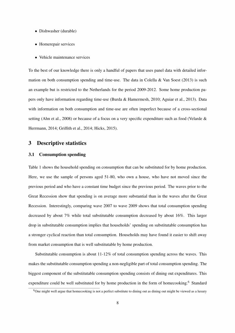
Table 1 shows the household spending on consumption that can be substituted for by home production.
Here, we use the sample of persons aged 51-80, who own a house, who have not moved since the
previous period and who have a constant time budget since the previous period. The waves prior to the
Great Recession show that spending is on average more substantial than in the waves after the Great
Recession. Interestingly, comparing wave 2007 to wave 2009 shows that total consumption spending
decreased by about 7% while total substitutable consumption decreased by about 16%. This larger
drop in substitutable consumption implies that households’ spending on substitutable consumption has
a stronger cyclical reaction than total consumption. Households may have found it easier to shift away
from market consumption that is well substitutable by home production.
Substitutable consumption is about 11-12% of total consumption spending across the waves. This
makes the substitutable consumption spending a non-negligible part of total consumption spending. The
biggest component of the substitutable consumption spending consists of dining out expenditures. This
expenditure could be well substituted for by home production in the form of homecooking.6 Standard
6One might well argue that homecooking is not a perfect substitute to dining out as dining out might be viewed as a luxury
8
deviations of the spending categories are relatively big compared to the mean. The relative size of
the standard deviation compared to the mean is much smaller for the total of consumption spending.
This suggest that there is especially large (cross-sectional) heterogeneity in consumption spending that
could be substituted for by home production activities. We observe that virtually all households have
expenditures that could be substituted for by home production.
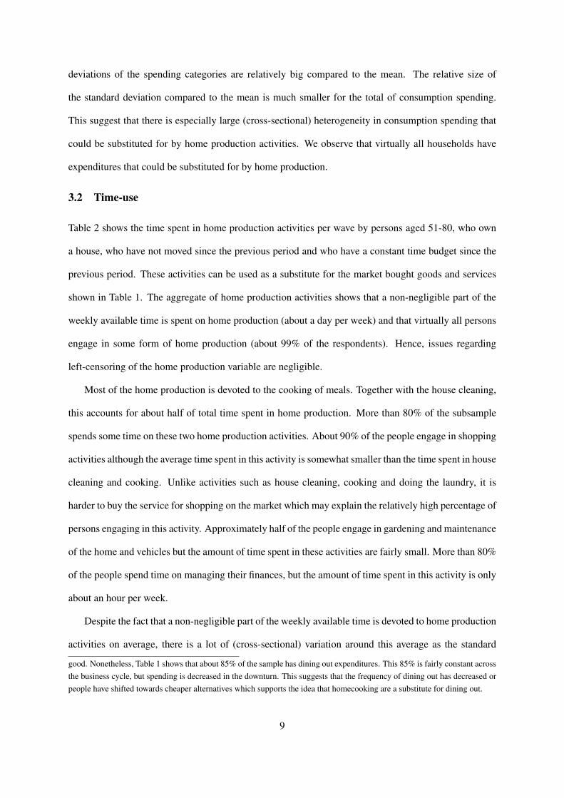
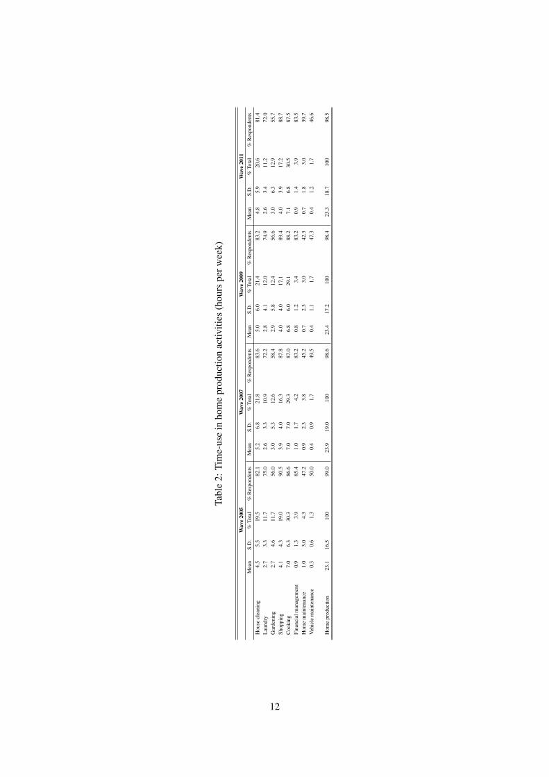
3.2 Time-use
Table 2 shows the time spent in home production activities per wave by persons aged 51-80, who own
a house, who have not moved since the previous period and who have a constant time budget since the
previous period. These activities can be used as a substitute for the market bought goods and services
shown in Table 1. The aggregate of home production activities shows that a non-negligible part of the
weekly available time is spent on home production (about a day per week) and that virtually all persons
engage in some form of home production (about 99% of the respondents). Hence, issues regarding
left-censoring of the home production variable are negligible.
Most of the home production is devoted to the cooking of meals. Together with the house cleaning,
this accounts for about half of total time spent in home production. More than 80% of the subsample
spends some time on these two home production activities. About 90% of the people engage in shopping
activities although the average time spent in this activity is somewhat smaller than the time spent in house
cleaning and cooking. Unlike activities such as house cleaning, cooking and doing the laundry, it is
harder to buy the service for shopping on the market which may explain the relatively high percentage of
persons engaging in this activity. Approximately half of the people engage in gardening and maintenance
of the home and vehicles but the amount of time spent in these activities are fairly small. More than 80%
of the people spend time on managing their finances, but the amount of time spent in this activity is only
about an hour per week.
Despite the fact that a non-negligible part of the weekly available time is devoted to home production
activities on average, there is a lot of (cross-sectional) variation around this average as the standard
good. Nonetheless, Table 1 shows that about 85% of the sample has dining out expenditures. This 85% is fairly constant acrossthe business cycle, but spending is decreased in the downturn. This suggests that the frequency of dining out has decreased orpeople have shifted towards cheaper alternatives which supports the idea that homecooking are a substitute for dining out.
9

Tabl
e1:
Hou
seho
ldle
velc
onsu
mpt
ion
spen
ding
(US
dolla
rspe
ryea
r)a
Wav
e20
05W
ave
2007
Wav
e20
09W
ave
2011
Mea
nS.
D.
%To
tal
%H
ouse
hold
sM
ean
S.D
.%
Tota
l%
Hou
seho
lds
Mea
nS.
D.
%To
tal
%H
ouse
hold
sM
ean
S.D
.%
Tota
l%
Hou
seho
lds
Din
ing
out
1,79
52,
996
4.5
89.2
1,76
12,
932
4.5
86.8
1,47
21,
959
4.1
86.8
1,68
32,
349
4.8
84.7
Hou
seke
epin
gse
rvic
es43
21,
407
1.1
49.9
390
1,23
01.
047
.529
192
70.
843
.629
685
70.
841
.6G
arde
ning
serv
ices
486
1,62
11.
241
.942
91,
235
1.1
40.2
348
803
1.0
42.7
363
830
1.0
43.2
Hom
erep
airs
ervi
ces
1,40
33,
587
3.5
59.5
1,41
23,
780
3.6
58.4
1,17
62,
720
3.3
54.5
1,05
93,
083
3.0
53.6
Veh
icle
mai
nten
ance
632
803
1.6
88.3
558
736
1.4
84.5
556
724
1.5
82.9
545
726
1.5
83.3
Dis
hwas
her
2110
70.
04.
524
113
0.0
4.8
1810
30.
03.
518
990.
03.
8W
ashi
ng/D
ryin
gm
achi
ne71
267
0.0
9.5
8229
40.
010
.369
278
0.0
9.1
4520
40.
08.
0
Subs
titut
able
cons
umpt
ion
4,84
15,
784
12.1
984,
656
6,09
712
.097
3,93
04,
402
10.9
974,
009
4,76
811
.397
Subs
titut
able
cons
umpt
ion
excl
.dur
able
s4,
749
5,75
811
.898
4,54
96,
069
11.7
973,
843
4,35
010
.697
3,94
64,
750
11.2
97Su
bstit
utab
leco
nsum
ptio
nin
cl.s
uppl
.mat
.6,
540
7,16
216
.310
06,
266
7,43
616
.199
5,32
05,
274
14.7
995,
402
5,94
015
.399
Tota
lcon
sum
ptio
n40
,120
28,1
4110
010
038
,856
26,4
5910
010
036
,122
23,1
5510
010
035
,348
21,2
4710
010
0
aM
onet
ary
mea
sure
sar
eex
pres
sed
in20
11U
Sdo
llars
usin
gth
eC
onsu
mer
Pric
eIn
dex
ofth
eB
urea
uof
Lab
orSt
atis
tics.
10
deviations of most activities are about the same size as the averages (or even bigger). However, the
variation across waves is only marginal despite the observed drop in substitutable market consumption
in Table 1. This might suggest that people do not adjust their time-use in home production that much as
a response to the consumption drops in the Great Recession.
Together, Table 2 and Table 1 give some cross-sectional evidence on the scope of substituting market
purchases for home production activities. To capture the possible substitution effects between the two
more formally, we present a theoretical framework including a simple life-cycle model augmented with
home production and wealth shocks in the next section. The theoretical framework justifies our empirical
identification method presented in Section 5 using within-person variation.
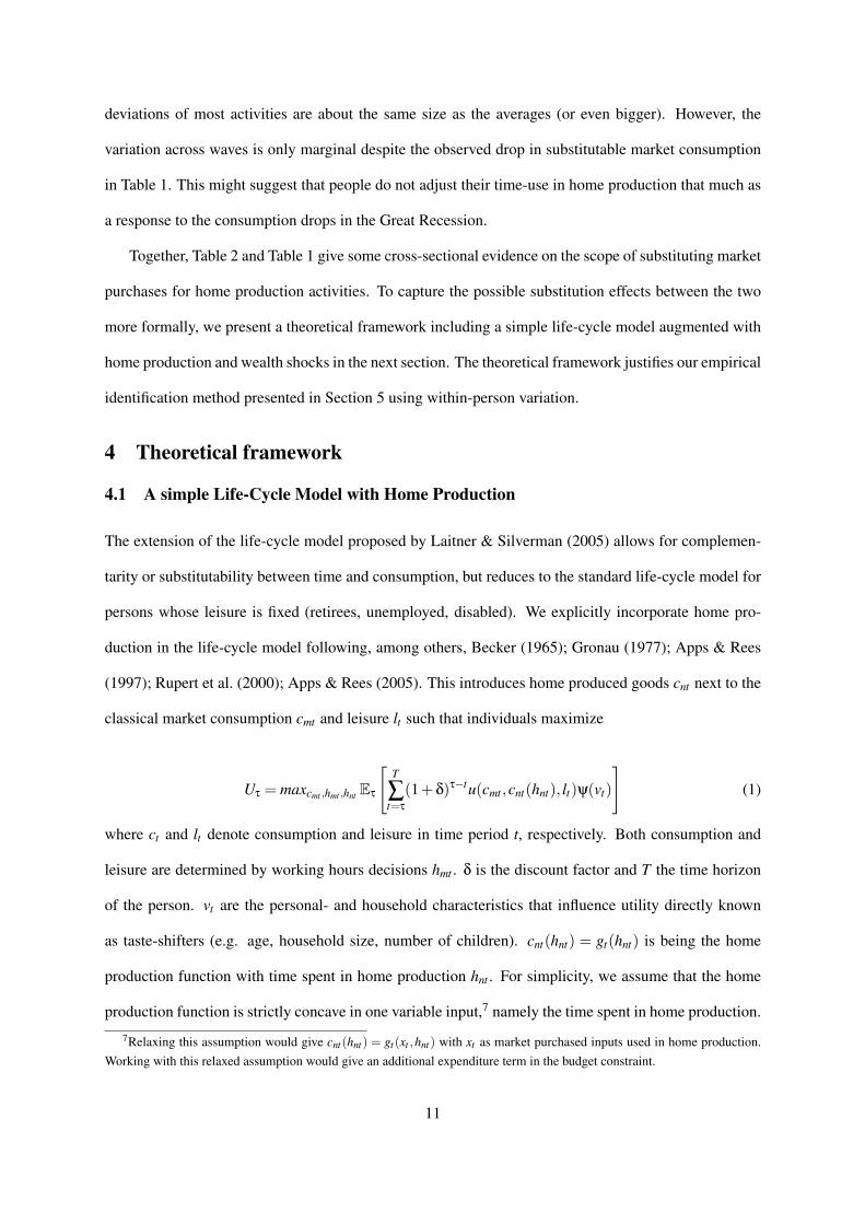
4 Theoretical framework
4.1 A simple Life-Cycle Model with Home Production
The extension of the life-cycle model proposed by Laitner & Silverman (2005) allows for complemen-
tarity or substitutability between time and consumption, but reduces to the standard life-cycle model for
persons whose leisure is fixed (retirees, unemployed, disabled). We explicitly incorporate home pro-
duction in the life-cycle model following, among others, Becker (1965); Gronau (1977); Apps & Rees
(1997); Rupert et al. (2000); Apps & Rees (2005). This introduces home produced goods cnt next to the
classical market consumption cmt and leisure lt such that individuals maximize
Uτ = maxcmt ,hmt ,hnt Eτ
[T
∑t=τ
(1+δ)τ−tu(cmt ,cnt(hnt), lt)ψ(vt)
](1)
where ct and lt denote consumption and leisure in time period t, respectively. Both consumption and
leisure are determined by working hours decisions hmt . δ is the discount factor and T the time horizon
of the person. vt are the personal- and household characteristics that influence utility directly known
as taste-shifters (e.g. age, household size, number of children). cnt(hnt) = gt(hnt) is being the home
production function with time spent in home production hnt . For simplicity, we assume that the home
production function is strictly concave in one variable input,7 namely the time spent in home production.
7Relaxing this assumption would give cnt(hnt) = gt(xt ,hnt) with xt as market purchased inputs used in home production.Working with this relaxed assumption would give an additional expenditure term in the budget constraint.
11
Tabl
e2:
Tim
e-us
ein
hom
epr
oduc
tion
activ
ities
(hou
rspe
rwee
k)
Wav
e20
05W
ave
2007
Wav
e20
09W
ave
2011
Mea
nS.
D.
%To
tal
%R
espo
nden
tsM
ean
S.D
.%
Tota
l%
Res
pond
ents
Mea
nS.
D.
%To
tal
%R
espo
nden
tsM
ean
S.D
.%
Tota
l%
Res
pond
ents
Hou
secl
eani
ng4.
55.
519
.582
.15.
26.
821
.883
.65.
06.
021
.483
.24.
85.
920
.681
.4L
aund
ry2.
73.
311
.775
.02.
63.
310
.972
.22.
84.
112
.074
.92.
63.
411
.272
.0G
arde
ning
2.7
4.6
11.7
56.0
3.0
5.3
12.6
58.4
2.9
5.8
12.4
56.6
3.0
6.3
12.9
55.7
Shop
ping
4.1
4.3
19.0
90.5
3.9
4.0
16.3
87.8
4.0
4.0
17.1
89.4
4.0
3.9
17.2
88.7
Coo
king
7.0
6.3
30.3
86.6
7.0
7.0
29.3
87.0
6.8
6.0
29.1
88.2
7.1
6.8
30.5
87.5
Fina
ncia
lman
agem
ent
0.9
1.3
3.9
85.4
1.0
1.7
4.2
83.2
0.8
1.2
3.4
83.2
0.9
1.4
3.9
83.5
Hom
em
aint
enan
ce1.
03.
04.
347
.20.
92.
33.
845
.20.
72.
33.
042
.30.
71.
83.
039
.7V
ehic
lem
aint
enan
ce0.
30.
61.
350
.00.
40.
91.
749
.50.
41.
11.
747
.30.
41.
21.
746
.6
Hom
epr
oduc
tion
23.1
16.5
100
99.0
23.9
19.0
100
98.6
23.4
17.2
100
98.4
23.3
18.7
100
98.5
12

Individuals maximize Equation 1 under the time budget and monetary budget constraint respectively
hmt = H− lt −hnt (2)
At+1 = (1+ r)(At +(wt ·hmt)+bt − cmt) (3)
AT ≥ 0 (4)
where At is the amount of assets at time t, r is a constant real interest rate, wt is the (after-tax) wage
rate, H the total time-endowment (e.g. 24 hours per day) and bt non-labor income (e.g. pensions,
unemployment benefits, disability benefits and other unearned non-asset income).
Since not all consumption spending categories can be substituted by home production (e.g. utilities,
drugs, etc.) we assume that market consumption bundle consists of a component that is substitutable
(csmt) and a component that is not (cns
mt).
cmt = {csmt ,c
nsmt} (5)
Additionally, we assume that hmt = 0. In this way, we only consider the corner solution of labor supply
or, more specifically, retired individuals. These retirees are most likely to respond to houseprice shocks
(Campbell & Cocco, 2007) and it can be assumed that the houseprice shock did not change the labor
supply decisions (see Section 5). So, basically we constrain the analysis to the maximization of utility
over the remaining life-time in retirement assuming retirement to be an absorbing state. Hence, the time
budget (2) and monetary budget (3) are reduced to:
hnt = H− lt (6)
At+1 = (1+ r)(At +bt − cmt) (7)
Solving equation 1 subject to equations 6 and 7 gives the following Euler Equations of marginal utility
with respect to hnt (home production) and cmt (market consumption).
13

ucmt (cmt ,cnt(hnt), lt)ψ(vt) =
(1+ r1+δ
)Et [ucmt+1(cmt+1,cnt+1(hnt+1), lt+1)ψ(vt+1)] (8)
uhnt (cmt ,cnt(hnt), lt)ψ(vt) = wt
(1+ r1+δ
)Et[uhnt+1(cmt+1,cnt+1(hnt+1), lt+1)ψ(vt+1)
](9)
where( 1+r
1+δ
)Et [ucmt+1(cmt+1,cnt+1(hnt+1), lt+1)ψ(vt+1)] captures the marginal utility of wealth. The
marginal utility of wealth takes into account all future expectations. Hence, the optimal level of con-
sumption of market goods is where the marginal utility of consumption of market goods equals the
marginal utility of wealth (taking into account a fixed interest rate and discount factor).
Similarly, the marginal utility of home production depends on the marginal utility of wealth as well
as the wage rate. A higher wage rate decreases the marginal utility of home production for which the
wage rate is an opportunity cost similar to leisure. The model predicts that the marginal utility of home
production is equal across different activities.
Expressions 8 and 9 imply that market consumption and home production are functions of the indi-
vidual’s current characteristics that determine the wage as well as all relevant information about other
periods, including future periods. Only an unanticipated shock, such as a shock in wealth, can result
into a deviation from the optimal path.
4.2 A simple Life-Cycle Model with Home Production and Wealth Shocks
Since we are explicitly interested in how a wealth shock affects home production through its effect on
the monetary budget constraint, we add a stochastic component to the deterministic life-cycle monetary
budget constraint in Equation 3.
At+1 = (1+ r)(Et [At ]+bt − cmt) (10)
with
Et [At ] = At +ξt (11)
14

Here, we assume that At = {A ft ,Ah
t } consists of both financial (A ft ) and housing wealth (Ah
t ). Although
financial wealth is more liquid, we assume that both are equally important in consumption decisions.
Campbell & Cocco (2007) argue that housing wealth is important for consumption decision primar-
ily through perceived wealth and borrowing constraints. For empirical evidence on the importance of
housing wealth for consumption decisions, see for example Case et al. 2005, 2013; Carroll et al. 2011;
Campbell & Cocco 2007; Angrisani et al. 2015; Christelis et al. 2015; Mian et al. 2013; Kaplan et al.
2016. This may especially be the case for our subgroup of retirees8 who generally tend to have a strong
bequest motive (Bernheim, 1991; Alessie et al., 1997, 1999; Skinner & Zeldes, 2002; Kopczuk & Lup-
ton, 2007) although in part these wealth holdings me be accidental (Hurd, 1989).9 Hence, shocks to
the value of the house can result in different consumption decisions. The theoretical framework also
assumes that housing is a pure investment good and that there is no consumption component to owning
a house.
ξt yields a shock in the value of wealth available at time t consisting of both permanent (ζt) and
transitory (ωt) shocks
ξt = ζt +ωt (12)
with persistence parameter of the permanent shock ρ and the permanent shock νt .
ζt = ρζt−1 +νt (13)
Both νt and ω are normally distributed. A negative shock (νt < 0) is unanticipated and has a permanent
effect on the life-time monetary budget constraint. As a consequence, it causes the future market con-
sumption possibilities cmt+p to decrease. Hence, retirees reoptimize hnt+p and cmt+p to the shock in the
monetary budget accordingly. Note that shocks to income and wealth are completely independent in this
theoretical framework. The theoretical framework predicts (∆cmt∆νt
> 0) (marginal propensity to consume)
and (∆hnt∆νt
< 0) (marginal propensity to produce at home) if ( ∆hnt∆cmt
< 0).
8Campbell & Cocco (2007) find that consumption responses to changes in houseprices increase with age.9This can also be explicitly modeled by allowing for a bequest function in the utility function. See, for example, Kopczuk
& Lupton (2007).
15

5 Empirical model
Much of the literature estimates the Euler equations by assuming a simple functional form10 of the utility
function and log-linearizing the parameterization (Rupert et al., 1995, 2000; Gortz, 2006). Since we are
only interested in the elasticity of home production with respect to market consumption, and not in the
particular levels, we use a reduced form approach that allows for identification of the elasticity. In order
to stay close to the structural equation modeling that uses log-linearization of the Euler equations, we
use a first-differences approach. An advantage of the first-difference specification is that the estimation
is not affected by possible individual fixed effects that may influence the levels of market consumption,
market work and home production (Parker, 1999).
Since it is expected that the intratemporal elasticity between non-substitutable market consumption
(cnsmt) and home production (cnt(hit)) is zero, we focus on the intratemporal elasticity between substi-
tutable market consumption (csmt) and home production. To estimate this elasticity between home pro-
duction and market consumption, we need to estimate
∆ln(hint+1) = ∆Xit+1βn1 +∆ln(csimt+1)βn2 + εint+1 (14)
where βn2 =∆hnt+1∆cs
mt+1is the elasticity between home production (hnt+1) and home production substitutable
consumption spending (csmt+1), X is a vector of control variables including individual- and household
characteristics, and ε is the error term which is distributed iid N(0,σh).
Here, hnt+1 and csmt+1 are simultaneously determined and therefore endogenous. Hence, estimates
of βn2 would be biased and we need a valid and relevant instrument, e.g. an instrument that affects
affects market consumption but not home production. Following our theoretical model in Section 4.2,
we argue that unexpected and persistent wealth shocks are both valid and relevant. A negative shock
in wealth decreases the market consumption possibilities ceteris paribus through the monetary budget
constraint (Equation 10), but it does not change the number of hours available for home production (the
time budget constraint, Equation 2). The effects of a wealth shock on home production run through its10More sophisticated functional forms are used in macro calibration exercises such as in Benhabib et al. (1991), Greenwood
& Hercowitz (1991), Fang & Zhu (2012), Dotsey et al. (2010), Rogerson & Wallenius (2013) and Karabarbounis (2014). Thesepapers use a Cobb-Douglas period utility function as a CES parameterization of the utility function with home production.
16

effect on decreased market consumption possibilities. Therefore, we propose the unexpected change in
(the log of) house prices due to the Great Recession (DGR∆ln(Wit)) as an instrumental variable capturing
ξt in Equation 11. Using a two-step IV-GMM with Equation 14 as the second-stage, we define the
first-stage as
∆ln(csimt+1) = ∆Xit+1βc1 +DGR∆ln(Wit)βc2 + εict+1 (15)
Angrisani et al. (2015) and Christelis et al. (2015) show that this unexpected and sufficiently large
and persistent shock decreased market consumption spending. In general it is found that consumption
responds to unexpected shocks in houseprices (Case et al., 2005, 2013; Carroll et al., 2011). Especially
among older households as these are most likely to gain and lose from houseprice changes (Campbell &
Cocco, 2007). Case et al. (2005) and Case et al. (2013) also argue that the sensitivity of consumption to
unexpected changes in housing wealth is greater than the sensitivity to unexpected changes in financial
wealth.
Compared to Kuehn (2015), who estimates a drop in houseprices directly on time spent in home pro-
duction, we explicitly use the fact that the effect of wealth runs through market consumption. Contrasting
Kuehn (2015) who uses state-level houseprice indices, we use individual-level houseprice values11 fol-
lowing Christelis et al. (2015). The average houseprices over the CAMS waves are shown in Figure 1.
The average year-to-year change in reported house prices is presented in Figure 2. The individual-level
change in the houseprice from 2007-2009 is used as the instrument in the IV-GMM regression. The
average reported houseprices follow a similar trend as other objective house price indices can be seen in
Figure 3.
To make sure that the wealth shock does not change the time budget because of consequences for
unemployment we estimate the model on the subsample of full retirees at time t and t +1 only. In this
way we make sure that ∆hmt+1 = 0, ∆wt+1 = 0 and ∆bt+1 = 0. For this sample of retirees, the mechanism
is most tractable. A shock in wealth decreases the monetary budget and, since the time budget does not
change, decreases market consumption possibilities by definition.
11From the RAND HRS Income and Wealth Imputation.
17

Figure 1: Development of houseprices
180
200
220
240
260
Mea
n re
port
ed h
ouse
pric
e (1
,000
’s o
f U.S
. dol
lars
)
2003 2005 2007 2009 2011Year
Source: HRS.
Figure 2: Year-to-year changes in houseprices
−20
−10
010
2030
Mea
n re
port
ed h
ouse
pric
e ch
ange
(1,
000’
s of
U.S
. dol
lars
)
2003 2005 2007 2009 2011Year
Source: HRS.
18

Figure 3: Development of houseprice indices
120
140
160
180
200
220
2003 2005 2007 2009 2011Year
U.S. House Price Index Case−Shiller Index (20 cities)
Source: Federal Housing Finance Agency (FHFA) and S&P Case-ShillerHome Price Indices.
We condition the elasticity on a set of observable personal- and household characteristics Xit+1.
This vector includes age effects, health effects, period effects, marital status as well as information
regarding the health and retirement statuses of the spouse.12 Due to our first-difference specification
we therefore condition on shocks in health13 and marital status.14 We combine quadratic age-effects
with semi-parametric age effects in the age of 62, 65 and 70.15 At these ages, people can claim Social
Security benefits at the earliest possible age, without actuarial reductions16 and the latest possible age
respectively.
12Estimation results are highly robust to excluding information regarding the spouse13Estimation results are highly robust to excluding changes in health.14Estimation results are highly robust to excluding changes in marital status.15Estimation results are highly robust to excluding such semi-parametric age effects.16The Full Retirement Age is 65 for all persons born before 1938.
19

6 Estimation results
6.1 Baseline estimates
Estimation results of the baseline specification are presented in Table 3 and indicate that the elasticity
between home production and substitutable consumption spending is -0.65.17 This means that a 10%
decrease in consumption spending that is substitutable for home production increases home production
by 6.5%. Home production is therefore found to be a (less than perfect) substitute for (substitutable)
market consumption.18
For comparison, the elasticity is bigger than the estimated elasticities of Hicks (2015) for Mexico
(0.049-0.064%) and the US (0.028-0.031%). It should, however, be noted that the estimated elastici-
ties of Hicks (2015) include prime age persons and are solely based on food consumption which is a
subgroup of our definition of home production substitutable consumption. Also, the econometric spec-
ification used by Hicks (2015) does not correct for simultaneity in consumption and home production
decisions. Neither does the specification of Hicks (2015) take into account possible changes in the time
budget.
The estimated elasticity is identified by the significant effect of the instrument DGR∆ln(Wit) on con-
sumption spending. More specifically, the estimated coefficient of the instrument implies that a 10%
decrease in the houseprice during the Great Recession decreased home production substitutable con-
sumption spending by 1.4%. This elasticity is somewhat bigger than the elasticity found by Christelis
et al. (2015) (0.56%). However, their elasticity is not recession-specific like ours, but accounts for the
whole time-span. Angrisani et al. (2015) estimate a non-recession and recession-specific elasticity. The
non-recession elasticity is not significant, the recession-specific elasticity is bigger than our elasticity
(about 4%). The elasticity found by Campbell & Cocco (2007) is most in line with our estimated elas-
ticity between market consumption and housing wealth (1.2%).
To facilitate the interpretation of the results, we can translate the effects into average effects for the
17The F-statistic of the excluded instrument is 5.6. Therefore, we test our estimation results with a Fuller-k estimator whichis more robust to possibly weak instruments. Estimation results of the elasticity are robust: -0.56*.
18The validity of our approach depends on keeping the time budget constant. Significance of the estimated elasticity disap-pears when we do not restrict the sample to persons with a constant time budget (not reported here). Running a simple OLSregression with potential endogeneity issues does not show a significant elasticity (not reported here).
20

sample of persons used in the regression analysis. Average consumption spending on home production
substitutable goods and services is 3,970 dollars per year. The average number of hours spent in home
production is 22.6 hours per week. The elasticity implies that, on average, a drop in consumption
spending of 40 dollars (per year) on home production substitutable market goods and services increases
home production activities by about 9 minutes per week or about 7.6 hours per year. The combination
of these facts imply a shadow price of about 5.30 dollars per hour. For comparison, this shadow price
is somewhat smaller than most minimum wages in the US, except for the states Georgia and Wyoming
(both 5.15 dollars p/h). A shadow price below the minimum wage seems quite plausible for the group
of retired persons as the reservation wage drops in retirement (Ghez & Becker, 1975).
The average houseprice in the year before the Great Recession is 223,563 dollars. A houseprice
drop of 2,235 dollars due to the Great Recession decreased home production substitutable consumption
spending by about 5.6 dollars in 2009 compared to 2007.
6.2 Sensitivity
Table 4 indicates that the results are robust to different consumption spending definitions. Consumption
excluding durables excludes the expenditures on a dishwasher and a washing and/or drying machine.
Consumption including supplementary material includes expenditures on home repair supplements,
housekeeping supplements and gardening supplements. Defining home production substitutable con-
sumption solely by dining out (e.g. the biggest potential spending category with a substantial drop from
2007 to 2009, on average (Table 1)) gives an elasticity that is much smaller than the aforementioned def-
initions of substitutable consumption (-0.29). This might be explained by the relatively large amount of
time spent on cooking, on average (Table 2). Hence, there might be little scope to increase the time spent
in cooking. Excluding maintenance to the house from the home production substitutable consumption
spending might be relevant as as the drop in houseprices might change the propensity to fix the house.
This is also suggested by the large drop in spending on homerepair services in Table 1. The elasticity
in which homerepair services are excluded is fairly similar to the baseline elasticity (-0.74). The same
applies to additionally excluding gardening services.
In the baseline regression we assumed full sharing of the household market consumption spending.
21

Table 3: Estimate of the elasticity be-tween consumption spending and homeproductiona
Second-stage ∆ln(hint+1)
Coeff. S.E.Control variables∆Age 0.46** 0.21∆Age2(/100) -0.27** 0.14∆1(Age≥ 62) 0.03 0.14∆1(Age≥ 65) -0.14 0.12∆1(Age≥ 70) -0.15* 0.09∆Health(−) 0.04 0.07∆Health(+) 0.05 0.08∆ Partner retired 0.01 0.06∆Health(−) partner 0.06 0.08∆Health(+) partner 0.03 0.09∆Single 0.99* 0.52∆Partner -0.15 0.25∆Wave2007 -0.29* 0.17∆Wave2009 -0.54* 0.32∆Wave2011 -0.84* 0.48
Elasticity∆ln(cs
imt+1) -0.65* 0.37
First-stage ∆ln(csimt+1)
Coeff. S.E.InstrumentDGR∆ln(Wit) 0.14** 0.06
Observations (N×T ) 2,500a * Significant at the .10 level; ** at the .05 level; *** at the
.01 level using t-statistics. Standard errors reported are robust toheteroskedasticity and autocorrelation. Time-use in Home Pro-duction includes: Housecleaning, Laundry, Gardening, Shopping,Cooking, Financial Management, Home improvements, Car im-provements. Consumption spending includes spending on: Vehi-cle maintenance, Dishwasher, Wash and drying machine, Homerepair services, Housekeeping services, Gardening services, Din-ing out. Time-use in Home Production and Consumption spend-ing are transformed using the inverse hyperbolic sine transforma-tion. Changes in Home Production and Consumption spending aretrimmed for the top and bottom 1 percent of the sample in eachsurvey wave following Angrisani et al. (2015); Hicks (2015). Thesample for the estimation consists of persons aged 51-80, who owna house, who have not moved since the previous period and whohave a constant time budget since the previous period.
22

Table 4: Elasticities with different definitions of (substitutable) consumption spendinga
Definition First-stage Second-stageβc2 σ2
βc2βn2 σ2
βn2Obs.
ln(csimt+1) 0.14** 0.06 -0.65* 0.37 2,500
ln(csimt+1) excl. durables 0.12** 0.06 -0.71* 0.44 2,500
ln(csimt+1) incl. suppl. material 0.14** 0.06 -0.61** 0.31 2,504
ln(csimt+1) dining out only 0.30*** 0.11 -0.29* 0.17 2,489
ln(csimt+1) excl. homerepair services 0.12** 0.06 -0.74* 0.45 2,491
ln(csimt+1) excl. homerepair/gardening services 0.12** 0.06 -0.74* 0.45 2,490
a * Significant at the .10 level; ** at the .05 level; *** at the .01 level using t-statistics. Standard errors reported are robust to heteroskedasticity andautocorrelation. Time-use in Home Production includes: Housecleaning, Laundry, Gardening, Shopping, Cooking, Financial Management, Home im-provements, Car improvements. Consumption spending includes spending on: Vehicle maintenance, Dishwasher, Wash and drying machine, Home repairservices, Housekeeping services, Gardening services, Dining out. Time use in Home Production and Consumption spending are transformed using theinverse hyperbolic sine transformation. Changes in Home Production and Consumption spending are trimmed for the top and bottom 1 percent of thesample in each survey wave following Angrisani et al. (2015); Hicks (2015). The sample for the estimation consists of persons aged 51-80, who own ahouse, who have not moved since the previous period and who have a constant time budget since the previous period. All regressions control for changesin age (including non-linearities), health, single/couple household, shocks to the partner and wave.
Nonetheless, the estimated elasticity is highly robust to a variety of equivalence scales to correct mar-
ket consumption spending such as the Oxford equivalence scale,19 OECD equivalence scale20 and the
Square root scale (all show an elasticity of about -0.65).21
Regarding individual- and household characteristics we find substantial differences in the estimated
elasticity between age-groups and health status (Table 5). We do not find such heterogeneous elasticities
for single versus couple households and males versus females (Table 5).
Different identification strategies to estimate the elasticity were proposed by Rupert et al. (1995)
and Hicks (2015). Using permanent income as an instrumental variable as proposed by Hicks (2015)
is not identified in our IV-GMM setting because permanent income is time-invariant. Rupert et al.
(1995) proposed using lagged consumption as an instrumental variable. Estimation results using this
identification method are shown in Table 6 and indicate an elasticity of zero.22 However, drawback of
19Assigning a value of 1 to the first household member and 0.7 to each additional adult.20Assigning a value of 1 to the first household member and 0.5 to each additional adult.21Dividing consumption spending by the square root of household size.22This applies to both subsamples including and excluding non-homeowners.
23

Table 5: Elasticities for subgroupsa
Subsample First-stage Second-stageβc2 σ2
βc2βn2 σ2
βn2Obs.
AgeAge ≤ 62 0.16*** 0.06 -0.63* 0.34 2,328Age ≤ 65 0.17*** 0.06 -0.57* 0.31 2,152Age ≤ 70 0.18** 0.08 -0.39 0.25 1,547Age ≤ 75 0.24* 0.14 -0.21 0.16 771
HealthFair or poor 0.22** 0.11 -0.32 0.25 689Non-poor 0.15** 0.06 -0.60* 0.34 2,309
HouseholdSingle 0.07 0.06 -0.64 0.91 989Couple 0.20* 0.11 -0.76 0.49 1,511
GenderMale 0.04 0.09 -3.74 7.94 917Female 0.16** 0.07 -0.43 0.31 1,583a * Significant at the .10 level; ** at the .05 level; *** at the .01 level using t-statistics.
Standard errors reported are robust to heteroskedasticity and autocorrelation. Time-usein Home Production includes: Housecleaning, Laundry, Gardening, Shopping, Cook-ing, Financial Management, Home improvements, Car improvements. Consumptionspending includes spending on: Vehicle maintenance, Dishwasher, Wash and dryingmachine, Home repair services, Housekeeping services, Gardening services, Diningout. Time use in Home Production and Consumption spending are transformed usingthe inverse hyperbolic sine transformation. Changes in Home Production and Con-sumption spending are trimmed for the top and bottom 1 percent of the sample in eachsurvey wave following Angrisani et al. (2015); Hicks (2015). The sample for the esti-mation consists of persons aged 51-80, who own a house, who have not moved sincethe previous period and who have a constant time budget since the previous period.
24

Table 6: Identification from laggedconsumptiona
Second-stage ∆ln(hint+1)
Coeff. S.E.Elasticity∆ln(cs
imt+1) -0.05 0.04
First-stage ∆ln(csimt+1)
Coeff. S.E.Instrument∆ln(cs
imt) -0.49*** 0.05
Observations (N×T ) 1,519a * Significant at the .10 level; ** at the .05 level; *** at the .01 level
using t-statistics. Standard errors reported are robust to heteroskedas-ticity and autocorrelation. Time-use in Home Production includes:Housecleaning, Laundry, Gardening, Shopping, Cooking, FinancialManagement, Home improvements, Car improvements. Consump-tion spending includes spending on: Vehicle maintenance, Dish-washer, Wash and drying machine, Home repair services, House-keeping services, Gardening services, Dining out. Time-use in HomeProduction and Consumption spending are transformed using the in-verse hyperbolic sine transformation. Changes in Home Productionand Consumption spending are trimmed for the top and bottom 1percent of the sample in each survey wave following Angrisani etal. (2015); Hicks (2015). The sample for the estimation consists ofpersons aged 51-80, who own a house, who have not moved sincethe previous period and who have a constant time budget since theprevious period.
this approach is that the instrument might not be valid as it is well-possible that persons with structurally
high levels of consumption spending generally engage less in home production. Our baseline estimates
are therefore preferred.
6.3 Heterogeneous elasticities
To get an idea of what drives the elasticity found in Table 3, Table 7 presents estimated elasticities for
a subsample of retirees with characteristics that might influence the strength of their home production
reactions to drops in substitutable market consumption. The estimated elasticity of the complementary
subsample of the regressions shown in Table 7 are not significantly different from zero.
The results suggest that much of the home production responses to drops in home production substi-
tutable market consumption found in Table 3 stem from persons who report a decline in their houseprice
value due to the Great Recession. Persons with a relatively low houseprice value prior to the recession
react more strongly than the average person. The same goes for the people that repaid their mortgage.
25
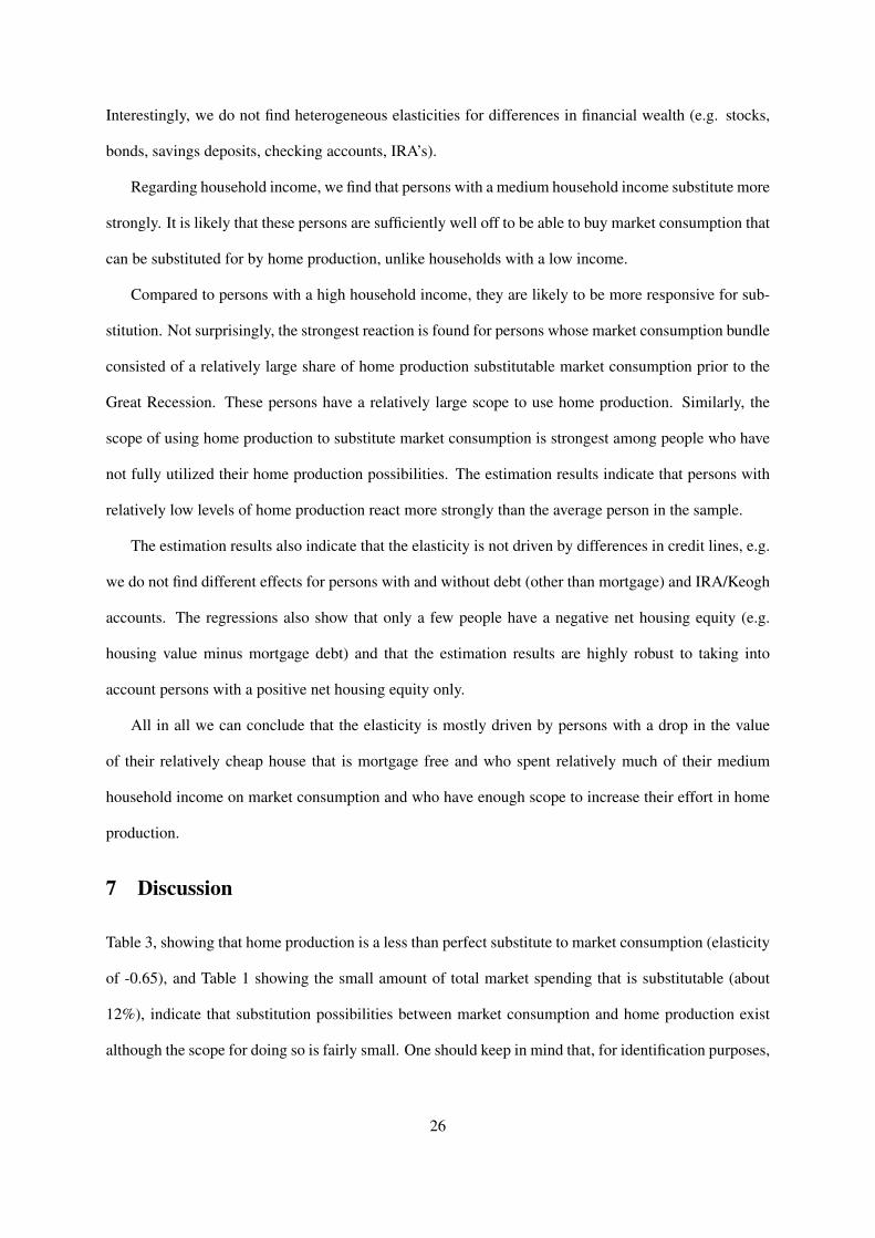
Interestingly, we do not find heterogeneous elasticities for differences in financial wealth (e.g. stocks,
bonds, savings deposits, checking accounts, IRA’s).
Regarding household income, we find that persons with a medium household income substitute more
strongly. It is likely that these persons are sufficiently well off to be able to buy market consumption that
can be substituted for by home production, unlike households with a low income.
Compared to persons with a high household income, they are likely to be more responsive for sub-
stitution. Not surprisingly, the strongest reaction is found for persons whose market consumption bundle
consisted of a relatively large share of home production substitutable market consumption prior to the
Great Recession. These persons have a relatively large scope to use home production. Similarly, the
scope of using home production to substitute market consumption is strongest among people who have
not fully utilized their home production possibilities. The estimation results indicate that persons with
relatively low levels of home production react more strongly than the average person in the sample.
The estimation results also indicate that the elasticity is not driven by differences in credit lines, e.g.
we do not find different effects for persons with and without debt (other than mortgage) and IRA/Keogh
accounts. The regressions also show that only a few people have a negative net housing equity (e.g.
housing value minus mortgage debt) and that the estimation results are highly robust to taking into
account persons with a positive net housing equity only.
All in all we can conclude that the elasticity is mostly driven by persons with a drop in the value
of their relatively cheap house that is mortgage free and who spent relatively much of their medium
household income on market consumption and who have enough scope to increase their effort in home
production.
7 Discussion
Table 3, showing that home production is a less than perfect substitute to market consumption (elasticity
of -0.65), and Table 1 showing the small amount of total market spending that is substitutable (about
12%), indicate that substitution possibilities between market consumption and home production exist
although the scope for doing so is fairly small. One should keep in mind that, for identification purposes,
26
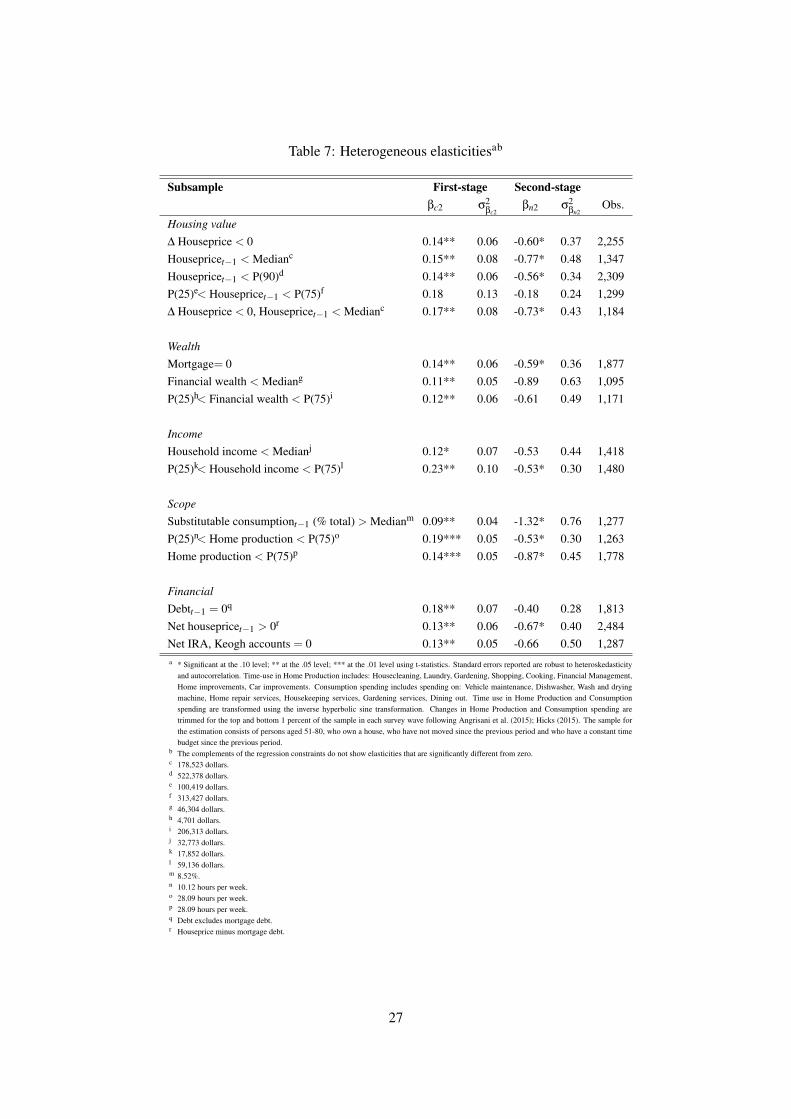
Table 7: Heterogeneous elasticitiesab
Subsample First-stage Second-stageβc2 σ2
βc2βn2 σ2
βn2Obs.
Housing value∆ Houseprice < 0 0.14** 0.06 -0.60* 0.37 2,255Housepricet−1 < Medianc 0.15** 0.08 -0.77* 0.48 1,347Housepricet−1 < P(90)d 0.14** 0.06 -0.56* 0.34 2,309P(25)e< Housepricet−1 < P(75)f 0.18 0.13 -0.18 0.24 1,299∆ Houseprice < 0, Housepricet−1 < Medianc 0.17** 0.08 -0.73* 0.43 1,184
WealthMortgage= 0 0.14** 0.06 -0.59* 0.36 1,877Financial wealth < Mediang 0.11** 0.05 -0.89 0.63 1,095P(25)h< Financial wealth < P(75)i 0.12** 0.06 -0.61 0.49 1,171
IncomeHousehold income < Medianj 0.12* 0.07 -0.53 0.44 1,418P(25)k< Household income < P(75)l 0.23** 0.10 -0.53* 0.30 1,480
ScopeSubstitutable consumptiont−1 (% total) > Medianm 0.09** 0.04 -1.32* 0.76 1,277P(25)n< Home production < P(75)o 0.19*** 0.05 -0.53* 0.30 1,263Home production < P(75)p 0.14*** 0.05 -0.87* 0.45 1,778
FinancialDebtt−1 = 0q 0.18** 0.07 -0.40 0.28 1,813Net housepricet−1 > 0r 0.13** 0.06 -0.67* 0.40 2,484Net IRA, Keogh accounts = 0 0.13** 0.05 -0.66 0.50 1,287a * Significant at the .10 level; ** at the .05 level; *** at the .01 level using t-statistics. Standard errors reported are robust to heteroskedasticity
and autocorrelation. Time-use in Home Production includes: Housecleaning, Laundry, Gardening, Shopping, Cooking, Financial Management,Home improvements, Car improvements. Consumption spending includes spending on: Vehicle maintenance, Dishwasher, Wash and dryingmachine, Home repair services, Housekeeping services, Gardening services, Dining out. Time use in Home Production and Consumptionspending are transformed using the inverse hyperbolic sine transformation. Changes in Home Production and Consumption spending aretrimmed for the top and bottom 1 percent of the sample in each survey wave following Angrisani et al. (2015); Hicks (2015). The sample forthe estimation consists of persons aged 51-80, who own a house, who have not moved since the previous period and who have a constant timebudget since the previous period.
b The complements of the regression constraints do not show elasticities that are significantly different from zero.c 178,523 dollars.d 522,378 dollars.e 100,419 dollars.f 313,427 dollars.g 46,304 dollars.h 4,701 dollars.i 206,313 dollars.j 32,773 dollars.k 17,852 dollars.l 59,136 dollars.m 8.52%.n 10.12 hours per week.o 28.09 hours per week.p 28.09 hours per week.q Debt excludes mortgage debt.r Houseprice minus mortgage debt.
27

Table 8: Substitution possibilities retirees and non-retireesa
hn csm
Mean S.E. Mean S.E.Non-retired 19.8 0.26 5,177.5 103.4Retired 23.2 0.23 3,747.8 64.0∆ 3.4*** 0.35 -1,429.7*** 115.3Non-retired men 16.1 0.29 6,013.6 175.9Retired men 19.1 0.23 3,992.8 96.3∆ 3.0*** 0.50 -2,020.7*** 194.9Non-retired women 22.6 0.39 4,540.6 122.1Retired women 25.2 0.28 3,624.5 83.0∆ 2.6*** 0.47 -916.0*** 143.1Non-retired < 65 19.4 0.27 5,247.1 133.6Retired < 65 23.6 0.47 3,766.0 126.9∆ 4.2*** 0.51 -1,481.1*** 199.2Non-retired 65+ 20.6 0.55 5,029.1 153.8Retired 65+ 23.0 0.27 3,740.8 73.9∆ 2.4*** 0.58 -1,288.3*** 158.6a * Significant at the .10 level; ** at the .05 level; *** at the .01 level using t-statistics.
this conclusion is based on a subsample of retired homeowners.
This specific subsample may have a different elasticity than non-retirees. The heterogeneous elas-
ticities in Table 7 suggest that persons who spent more of their total budget on market consumption that
is substitutable have a relatively big elasticity. Also, persons with a relatively small amount of time
spent on home production have a relatively big elasticity. These results imply that the endowment of
consumption and home production has consequences for the elasticity. Since retirees are expected to
be more well-endowed in terms of home production than non-retirees (because of total non-work time
available), it is expected that non-retirees may have a bigger elasticity.
By comparing groups of retirees and non-retirees, Table 8 confirms that retirees have higher levels
of home production and non-retirees have higher levels of substitutable market consumption. Based on
these descriptives non-retirees have a bigger scope to increase home production when necessary. Hence,
it is highly likely that the sample of non-retirees have a bigger elasticity than retirees since retirees have
used more of their substitution possibilities. The elasticity estimated in this paper can therefore be seen
as a lower bound of the elasticity for the whole population. However, it should also be kept in mind that
non-retirees have more possibilities to smooth shocks in income by adjusting their labor supply decision.
28

8 Conclusion
The theory of home production suggests that people will substitute away from market consumption as
the opportunity cost of time drops (Becker, 1965). Shifting away from market consumption to home
production makes people able to smooth consumption in response to income decreases (Hicks, 2015).
This is relevant as home production might be used to mitigate the consequences of shocks for well-being
(Aguiar & Hurst, 2005).
Prior studies have found that people respond to shocks in unemployment (Aguiar et al., 2013), health
(Gimenez-Nadal & Ortega-Lapiedra, 2013), retirement (Aguiar & Hurst, 2005) or wealth (Kuehn, 2015)
by increasing their home production. Shocks in retirement, unemployment and disability have two si-
multaneous effects 1) it decreases the monetary budget and 2) it increases the time budget. Therefore, the
extent to which home production is a substitute to market consumption remains unclear as the increases
in home production might be due to considerable increases non-work time available.
Compared to these prior studies, the current paper estimates the intratemporal elasticity between
home production and consumption spending from within-person variation. Earlier attempts to esti-
mate the intratemporal elasticity econometrically are based on subsamples of single women (Gelber
& Mitchell, 2012; Gonzalez Chapela, 2011), use debatable instruments (Rupert et al., 1995) or use
between-person variation (Hicks, 2015). We propose using a wealth shock as instrumental variable as
shocks in wealth affect the monetary budget constraint (e.g. market consumption) but not the time bud-
get constraint (e.g. home production). More specifically, we use the persistent and unanticipated shock
in houseprices during the Great Recession (Christelis et al., 2015; Angrisani et al., 2015; Kuehn, 2015)
to identify the elasticity. To exclude any possible effects of the Great Recession on the non-market time
available, we estimate elasticities for retirees only.
We find that a 10% decrease in substitutable market consumption increases the time spent in home
production activities by about 6.5%. The elasticity implies that a part of the decreased market con-
sumption possibilities can be replaced by home production to mitigate the consequences of shocks for
well-being. The scope for doing so remains rather limited, however. Home production substitutable
market consumption makes up 12% of total market consumption, on average, which makes it small but
29

non-negligible. The elasticity we find is largely driven by persons with a drop in the value of their
relatively cheap home, that is free of mortgage, and who spent relatively much of their medium house-
hold income on market consumption that can be substituted for by home production prior to the Great
Recession.
The micro elasticity estimated is much lower than the typically assumed high substitutability be-
tween market consumption and home production in existing macro models (Campbell & Ludvigson,
2001). This, however, does not need to be inconsistent (Chang & Kim, 2006). Also, it should be kept
in mind that our results are identified by a sample of retirees. Responses of prime age workers may be
different as their endowments in home production and substitutable market consumption are different.
Our elasticity is therefore to be seen as a lower bound for the whole population.
References
Aguiar, M., & Hurst, E. (2005). Consumption versus expenditure. Journal of Political Economy, 113(5),919–948.
Aguiar, M., Hurst, E., & Karabarbounis, L. (2012). Recent developments in the economics of time use.Annual Review of Economics, 4, 373–397.
Aguiar, M., Hurst, E., & Karabarbounis, L. (2013). Time use during the Great Recession. AmericanEconomic Review, 103, 1664–1696.
Aguila, E., Attanasio, O., & Meghir, C. (2011). Changes in consumption at retirement: Evidence frompanel data. Review of Economics and Statistics, 3, 1094–1099.
Ahn, N., Jimeno, J., & Ugidos, A. (2008). ”Mondays at the sun”: Unemployment, time-use, andconsumption patterns in Spain. (FEDEA Working Paper Paper, No. 2003-18)
Alessie, R., Lusardi, A., & Aldershof, T. (1997). Income and wealth over the life cycle: Evidence frompanel data. Review of Income and Wealth, 43, 729–758.
Alessie, R., Lusardi, A., & Kapteyn, A. (1999). Saving after retirement: Evidence based on threedifferent savings measures. Labour Economics, 6, 729–758.
Altonji, J. (1986). Intertemporal substitution in labor supply: Evidence from micro data. Journal ofPolitical Economy, 94, S176–S215.
Angrisani, M., Hurd, M., & Rohwedder, S. (2015). The effect of housing and stock wealth losses onspending in the Great Recession. (RAND Working Paper, No. WR-1101)
30
Apps, P., & Rees, R. (1997). Collective labour supply and household production. Journal of PoliticalEconomy, 105, 178–190.
Apps, P., & Rees, R. (2005). Gender, time use, and public policy over the life-cycle. Oxford Review ofEconomic Policy, 21, 439–461.
Banks, J., Blundell, R., & Tanner, S. (1998). Is there a retirement-savings puzzle? American EconomicReview, 88(4), 769–788.
Battistin, E., Brugiavini, A., Rettore, E., & Weber, G. (2009). The retirement consumption puzzle:Evidence from a regression discontinuity approach. American Economic Review, 99, 2209–2226.
Baxter, M., & Jermann, U. (1999). Household productivity and the excess sensitivity of consumption tocurrent income. American Economic Review, 89, 902–920.
Becker, G. (1965). A theory of the allocation of time. The Economic Journal, 75, 493–517.
Benhabib, J., Rogerson, R., & Wright, R. (1991). Homework in macroeconomics: Household produc-tion and aggregate fluctuations. Journal of Political Economy, 99, 1166–1187.
Bernheim, B. (1991). How strong are bequest motives? Evidence based on estimates of the demand forlife insurance and annuities. Journal of Political Economy, 99, 899–927.
Bernheim, B., Skinner, J., & Weinberg, S. (2001). What accounts for the variation in retirement wealthamong US households? American Economic Review, 91(4), 832–857.
Burda, M., & Hamermesh, D. (2010). Unemployment, market work and household production. Eco-nomics Letters, 107, 131–133.
Campbell, J., & Cocco, J. (2007). How do house prices affect consumption? Evidence from micro data.Journal of Monetary Economics, 54, 591–621.
Campbell, J., & Ludvigson, S. (2001). Elasticities of substitution in Real Business Cycle models withhome production. Journal of Money, Credit, and Banking, 33, 847–875.
Carroll, C., Otsuka, M., & Slacalek, J. (2011). How large are housing and financial wealth effects? Anew approach. Journal of Money, Credit and Banking, 43, 55–79.
Case, K., Quigley, J., & Shiller, R. (2005). Comparing wealth effects: The stock market versus thehousing market. Advances in Macroeconomics, 5, 1–34.
Case, K., Quigley, J., & Shiller, R. (2013). Wealth effects revisited 1975-2012. Critical Finance Review,2, 101–128.
Chang, Y., & Kim, S. (2006). From individual to aggregate labor supply: A quantitative analysis basedon a heterogeneous agent macroeconomy. International Economic Review, 47, 1–27.
Christelis, D., Georgarakos, D., & Jappelli, T. (2015). Wealth shocks, unemployment shocks andconsumption in the wake of the Great Recession. Journal of Monetary Economics, 72, 21–41.
31

Colella, F., & Van Soest, A. (2013). Time use, consumption expenditures and employment status:Evidence from the LISS panel. (Paper presented at the 7th MESS Workshop)
Dotsey, M., Li, W., & Yang, F. (2010). Consumption and time use over the life-cycle. (Federal ReserveBank of Philadelphia Research Department Working Paper, No. 10-37)
Fang, L., & Zhu, G. (2012). Home production technology and time allocation - empirics, theory andimplications. (mimeo)
Gelber, A., & Mitchell, J. (2012). Taxes and time allocation: Evidence from single women and men.Review of Economic Studies, 79, 863–897.
Ghez, G., & Becker, G. (1975). The allocation of time and goods over the life cycle. New York:Columbia University Press.
Gimenez-Nadal, J., & Ortega-Lapiedra, R. (2013). Health status and time allocation in spain. AppliedEconomics Letters, 20(15), 1435–1439.
Gonzalez Chapela, J. (2011). Recreation, home production, and intertemporal substitution of femalelabor supply: Evidence on the intensive margin. Review of Economic Dynamics, 14, 532–548.
Gortz, M. (2006). Heterogeneity in preferences and productivity - implications for retirement. (Leisure,household production, consumption and economic well-being, Ph.D. thesis, Chapter 4)
Greenwood, J., & Hercowitz, Z. (1991). The allocation of capital and time over the business cycle.Journal of Political Economy, 99, 1188–1214.
Greenwood, J., Rogerson, R., & Wright, R. (1995). Household production in Real Business Cycletheory. In T. Cooley (Ed.), Frotniers of Business Cycle research (p. 157-174). Princeton: PrincetonUniversity Press.
Griffith, R., O’Connell, M., & Smith, K. (2014). Shopping around? How households adjusted foodspending over the Great Recession. (paper presented at the EEA-ESEM 2014, Toulouse)
Gronau, R. (1977). Leisure, home production and work - the theory of the allocation of time revisited.Journal of Political Economy, 85, 1099–1124.
Guler, B., & Taskin, T. (2013). Does unemployment insurance crowd out home production? EuropeanEconomic Review, 62, 1–16.
Hall, R. (2009). Reconciling cyclical movements in the marginal value of time and the marginal productof labor. Journal of Political Economy, 117, 281–323.
Halliday, T., & Podor, M. (2012). Health status and the allocation of time. Health Economics, 21,514–527.
Hicks, D. (2015). Consumption volatility, marketization, and expenditure in an emerging market econ-omy. American Economic Journal: Macroeconomics, 7(2), 95–123.
32
Hurd, M. (1989). Mortality risks and bequests. Econometrica, 57, 779–813.
Hurd, M., & Rohwedder, S. (2007). Time-use in the older population. variation by socio-economicstatus and health. (RAND Labor and Population Working Paper Series, No. WP-463)
Hurd, M., & Rohwedder, S. (2008). The adequacy of economic resources in retirement. (MRRCWorking Paper Series, No. WP2008-184)
Hurd, M., & Rohwedder, S. (2009). Methodological innovations in collecting spending data: The HRSConsumption and Activities Mail Survey. Fiscal Studies, 30(3/4), 435–459.
Hurd, M., & Rohwedder, S. (2013). Heterogeneity in spending change at retirement. The Journal of theEconomics of Aging, 1-2, 60–71.
Hurst, E. (2008). The retirement of a consumption puzzle. (NBER Working Paper Series, No. 13789)
Kaplan, G., Mitman, K., & Violante, G. (2016). Non-durable consumption and housing net worth in theGreat Recession: Evidence from easily accessible data. (mimeo)
Karabarbounis, L. (2014). Home production, labor wedges, and international business cycles. Journalof Monetary Economics, 64, 68–84.
Kopczuk, W., & Lupton, J. (2007). To leave or not to leave: The distribution of bequest motives. Reviewof Economic Studies, 74, 207–235.
Krueger, A., & Mueller, A. (2012). Time use, emotional well-being, and unemployment: Evidence fromlongitudinal data. American Economic Review: Papers & Proceedings, 102, 594–599.
Kuehn, D. (2015). Home production, house values, and the great recession. Journal of Family andEconomic Issues, DOI 10.1007/s10834-015-9438-3.
Laitner, J., & Silverman, D. (2005). Estimating life-cycle parameters from consumption behavior atretirement. (NBER Working Paper Series, No. 11163)
Mariger, R. (1987). A life-cycle consumption model with liquidity constraints: Theory and empiricalresults. Econometrica, 55, 533–557.
Mian, A., Rao, K., & Sufi, A. (2013). Household balance sheets, consumption, and the economic slump.The Quarterly Journal of Economics, 128, 1687–1726.
Miniaci, R., Monfardini, C., & Weber, G. (2003). Is there a retirement-consumption puzzle in Italy?(Institute for Fiscal Studies Working Paper Series, No. 03/14)
Mroz, T. (1987). The sensitivity of an empirical model of married women’s hours of work to economicand statistical assumptions. Econometrica, 55, 765–799.
Parker, J. (1999). The reaction of household consumption to predictable changes in social security taxes.American Economic Review, 89, 959–973.
33

Robb, A., & Burbidge, J. (1989). Consumption, income, and retirement. Canadian Journal of Eco-nomics, 22, 522–542.
Rogerson, R., & Wallenius, J. (2013). Nonconvexities, retirement, and the elasticity of labor supply.American Economic Review, 103, 1445–1462.
Rupert, P., Rogerson, R., & Wright, R. (1995). Estimating substitution elasticities in household produc-tion models. Economic Theory, 6, 179–193.
Rupert, P., Rogerson, R., & Wright, R. (2000). Homework in labor economics: Household productionand intertemporal substitution. Journal of Monetary Economics, 46, 557–579.
Schwerdt, G. (2005). Why does consumption fall at retirement? Evidence from Germany. EconomicsLetters, 89, 300–305.
Skinner, J., & Zeldes, P. (2002). The importance of bequests and life-cycle savings in capital accumu-lation: A new answer. American Economic Review, 92, 274–278.
Stancanelli, E., & Van Soest, A. (2012). Joint leisure before and after retirement: A double regressiondiscontinuity approach. (IZA Discussion Paper, No. 6698)
Taskin, T. (2011). Unemployment insurance and home production. (MPRA Working Paper, No. 34878)
Velarde, M., & Herrmann, R. (2014). How retirement changes consumption and household productionof food: Lessons from German time-use data. The Journal of the Economics of Aging, 3, 1–10.
34
Top Related