


Languages
Pages
Legal


HIV/AIDS, ARV Treatment and Worker Absenteeism:Evidence from a Large African Firm ∗
James Habyarimana†, Bekezela Mbakile‡and Cristian Pop-Eleches§
First Draft - February 2007This Draft - April 2007 - Please do not cite/circulate
Abstract
In 2001, the Debswana Diamond Company started the first firm-basedprogram in Africa to provide free ARV treatment to its workforce affected byHIV/AIDS. We link individual health information from the firm’s treatment pro-gram to a unique panel dataset of all the medical and non-medical episodes of ab-senteeism at the firm’s two main mines between the period 1998-2006. This uniquedataset allows us to characterize medium and long-run impacts of the disease andARV treatment that existing data cannot address. Compared to workers that neverenroll in the treatment program, there is no statistically significant difference inthe absenteeism rate of enrolled workers in the period 1-5 years prior to treatmentstart. Next we present robust evidence of an inverse-V pattern in worker absen-teeism around the time of ARV treatment inception. Enrolled workers miss about20 days in the year leading up to treatment initiation with a peak of 5 days in thelast month. This is about five times the annual absence duration due to illnessamong non-enrolled workers. The introduction of ARV treatment is followed by alarge reduction in absenteeism 6-12 months following treatment inception. Absen-teeism 1 to 4 years after treatment start is low and similar to non-enrolled workersat the firm.Finally, we present a simple model to understand the conditions under which it
is optimal for profit-maximizing firms to finance/provide ARV treatment to theirworkers. Under plausible assumptions, our results suggest that for the typical man-ufacturing firm across East and Southern Africa, the benefits of treatment to thefirm cover between 10-33% of the cost of treatment.
∗We would like to thank Janet Currie, Josh Graff Zivin, Ted Joyce, Sarah Reber, Andrei Shleifer, Har-sha Thirumurthy, Eric Verhoogen and seminar participants at the Brookings Institution, Case Western,Cuny-NBER Health Seminar and Columbia for helpful comments.
†Georgetown University, Public Policy Institute, e-mail: [email protected]‡Debswana Diamond Company, HR Planning Superintendent, e-mail: [email protected]§Columbia University, Department of Economics and SIPA, e-mail: [email protected]
1

1 Introduction
Over 40 million people worldwide are infected with the HIV virus. More than 60% of
these individuals reside in Africa. One of the challenges of characterizing the impact of
the disease on a variety of socio-economic outcomes is the slow progression of the disease.
Shortly after an individual is infected, a long latency period follows that can last 8-10
years in which the individual is asymptomatic despite a gradual weakening of the immune
system.1 Eventually the individual develops full-blown AIDS and presents a wide variety
of opportunistic infections which in the absence of treatment lead to death within less
than 1 year.2
Over the last five years, numerous international organizations as well as national gov-
ernments have committed significant resources for the provision of antiretroviral drugs
(ARV’s) for the treatment of HIV/AIDS infected individuals in the developing world.
And although the ambitious goal of providing ARVs to 3 million patients around the
world by 2005 has not been achieved, the rate of increase has been large, even in Africa
where the number of patients on ARVs increased from 100,000 in 2003 to 810,000 in 2005
(UNAIDS, 2006).
The health benefits of ARVs are by now well established in the developed world (Ham-
mer et al. (1997), Duggan and Evans (2005), Floridia et al. (2002)) and recently a number
of papers have also shown large reductions in morbidity and mortality in the first years af-
ter treatment start in poor country settings (Koenig et al. (2004), Wools-Kaloustian et al
(2006).3 Despite these positive health effects, there is little evidence on the socio-economic
effects of HIV/AIDS and ARVs on individuals, households and firms. Two notable excep-
tions are Thirumurthy et al (2005) who find sizable increases in labor supply in patients
in the first six to nine months after initiation of treatment in a sample of rural households
in Kenya, and Fox et al (2004) who document decreases in worker productivity among
rural Kenyan tea pickers in the last two years prior to leaving the firm for AIDS related
1In the US, the median latency period is 10 years (NIH, 2005) and evidence from Uganda suggeststhat this is similar in an African setting (Morgan et al. 2002).
2The median time from AIDS to deaths in the absence of treatment in the Ugandan study was 9.2months (Morgan et al. 2002).
3Marins et al.(2003) using a longitudinal data from Brazil find that median survival time increased to58 months for patients on ARVs.
2

sickness or death.4 Apart from the intrinsic interest of elucidating the relationship be-
tween health and socio-economic behavior (Strauss and Thomas (1998), Case and Deaton
(2006), Thomas et al. (2005)),5 understanding the additional socio-economic benefits of
ARV treatment can shed light on the cost-effectiveness of antiretroviral drugs (ARVs) in
comparison with available HIV/AIDS prevention interventions. Despite the documented
health benefits and the recent reduction of the cost of treatment, the cost-effectiveness
of ARV treatment in the context of the developing world has recently been questioned
(Canning (2006)).
While the aforementioned studies have shown significant changes in the labor supply of
infected workers in the late stages of the disease as well as patients who have just started
ARV therapy, little is known about how morbidity affects socio-economic behavior in the
longer term. In this paper we focus on the medium and long term economic impacts of
HIV/AIDS and benefits of ARV treatment. More specifically we analyze the pattern of
labor market absenteeism of workers with HIV/AIDS in the years prior to and following
the start of ARV treatment, using detailed human resource data spanning a period of
almost 10 years from a major private mining firm in Botswana. In 2001, the Debswana
Diamond Company, Botswana’s main diamond mining enterprise, with a workforce of
over 6500,6 started one of the first free firm-based ARV treatment programs to extend
the productive lives of its workers. The decision to provide treatment came as a response
to an HIV/AIDS prevalence rate among its workforce of 28% in 1999 and increases in
HIV/AIDS related deaths, early retirement and absenteeism (UNAIDS, 2006).
We carry out our analysis by linking a database of the entire universe of regular and
sickness related spells of absenteeism at the firm’s two main mining sites with information
about the health status and timing of ARV treatment start for a group of almost 500
workers enrolled in the company’s treatment program. The absenteeism data covers the
4A number of macro-economic studies of the impact of the epidemic on economic growth reach con-flicting conclusions. Young (2005) posits positive effects via changes in fertility while Bell, Devarajanand Gersbach (2003) and Kalemli-Ozcan (2006) posit negative effects.
5In addition to the micro based studies on the relationship between health and socio-economic out-comes, a number of cross country studies have focussed on the relationship between health and growth(Sachs (2003), Acemoglu and Johnson (2006)).
6Debswana is an unusually large African firm. The average firm size in the manufacturing sector ofmany African countries is about 120 employees and the median is about 40-50 employees (InvestmentClimate Assessment Reports (Kenya (2004), Uganda (2003) and Tanzania (2003)).
3

period 1998-2006 for the Jwaneng mine and the period 2001-2006 for the Orapa mine.
Since the Debswana treatment program was one of the first to be started in Africa and
the absenteeism data covers such a long time span, we are in a unique position to observe
the labor market behavior of workers with HIV/AIDS up to 5 years prior to and following
the initiation of ARV therapy.
We first provide evidence on the link between the health status of a worker (measured
by his/her CD4 count) and worker absenteeism in a given month, using measurements
of the CD4 count at 0, 6 and 12 months after treatment start.7 We propose to address
the potential endogeneity of health in the worker absenteeism equation by using the
length of time between the date of ARV treatment inception and the date of the CD4
count measurement as an instrumental variable for a person’s health. Our instrumental
variables estimate implies that within the first year of treatment, an increase equal to 100
cells/mL of the CD4 count (the average improvement in health after 6 months of therapy)
causes illness-related absenteeism to decrease by roughly 3.5 days per month.
Secondly, we use the staggered timing of worker treatment initiation between 2001 and
April 2006 to estimate the patterns of absenteeism around the start of ARV treatment
inception. The four main results of our empirical analysis are the following: (1) compared
to non-enrolled workers in the firm, we find no difference in the rate of absenteeism of
workers with HIV/AIDS in the period of 1-5 years prior to the start of treatment; (2) about
12-15 month prior to the start of treatment we observe a sharp increase in absenteeism
equivalent to about 20 days in the year prior to the start of treatment and with a peak
of 5 days in the month of treatment initiation; (3) the recovery after the beginning of
treatment happens quickly within the first year and (4) 1-4 years after treatment start,
treated workers display very low rates of absenteeism, similar to the other workers at the
mining company.
Next we develop a framework to predict the conditions under which firms will provide
ARV treatment to their workers. The framework, which builds on the literature on the
provision of firm-specific human capital (Becker (1964), Acemoglu and Pischke (1999)),
7The CD4 count is a measure of the density of CD4 cells — cells that are crucial in the body’s immuneresponse mechanism. While there is no reference normal range, CD4 counts >500 cells/ml are consideredhealthy (Kaufmann et. al. 2002). This is a suitable measure of underlying health as it provides directmeasure of the susceptibility of the body to infection.
4

shows that when the productivity differences between healthy experienced workers and
new recruits is small, firms prefer to hire new workers rather than provide treatment
to infected workers. Conversely when the productivity gains associated with treatment
(keeping experienced workers) are large, firms are more likely to provide treatment. We
provide a rationale for when, where and how much firms in Sub-Saharan Africa are willing
to pay towards the cost of treatment. We show that given the current costs of provision
of ARV’s and a number of plausible assumptions about the labor market, the turnover of
sick and treated workers, the benefits to the firm cover about 10-33% of the cost of ARV
treatment. We conclude that the provision of public subsidies to ARV treatment programs
administered by private companies has the potential to become an important mechanism
to provide treatment to people affected by HIV/AIDS in a resource constrained setting
like Africa.
Our analysis proceeds as follows. We describe Debswana’s company based treatment
program in Section 2. In Section 3, we introduce our data, empirical strategy and regres-
sion framework. Section 4 presents the results of the main analysis. Section 5 presents a
simple model to understand the impact of HIV/AIDS and ARV treatment for the company
and provides a rationale for firm-based treatment provision. Section 6 concludes.
2 The ARV treatment program at the Debswana Di-
amond Company8
Our analysis evaluates the impact of ARV treatment on labor market outcomes of
workers with HIV/AIDS at the Debswana Diamond Company in Botswana. Located
in Southern Africa, Botswana is considered an African success story given its political
stability and continued economic growth since independence. Despite these economic and
political achievements, the country has been hard hit by the HIV/AIDS epidemic with
an adult HIV prevalence rate of 24% in 2005 (UNAIDS, 2006) and a life expectancy at
birth of only 36 years.
8Unless otherwise noted, this section draws heavily on UNAIDS (2002)
5

The country’s economic success is closely linked to the fact that Botswana is the largest
producer of diamonds in the world. The company that is responsible for the diamond
mining activities is the Debswana Diamond Company, a 50-50 joint venture between the
Government of Botswana and the DeBeers Company. Employing more than 6,500 workers,
it plays an important role in Botswana’s economy and is by far the country’s largest
private employer. From its four major mining sites at Letlhakane, Jwaneng, Damtshaa
and Orapa, the company provides about 60% of the government’s revenue, accounts for
approximately 33% of Botswana’s GDP and over 80% of the country’s export earnings.
Relative to other large firms in Africa, Debswana has been a pioneer in sustained and
effective firm-based responses to the HIV/AIDS epidemic. Following the report of the first
AIDS case at the Jwaneng Mine Hospital in 1987, the company started an HIV/AIDS
education and awareness program in 1988. Starting in the mid 1990’s, the effect of the
epidemic on the morbidity and mortality of the company’s workforce became increasingly
conspicuous as the percentage of ill-health retirements due to HIV/AIDS rose to 75%
in 1999 and the number of deaths due to AIDS increased to 59% in the same year. In
1999, the HIV prevalence rate based on the first voluntary anonymous prevalence survey
conducted by the company was 28%. The prevalence rate from a similar survey in 2003
continued to be high (19.9%) and was higher among workers aged 30-39 (26%) and among
the unskilled and semi skilled workforce (23%).9
In May 2001, Debswana Diamond Company started an ambitious treatment program
that provides free antiretroviral therapy (ARVs) to the company’s workforce and their
spouses. The program has been extremely successful and enrolled 158 patients in the first
year of operation and that number has increased to over 700 by April 2006. According
to recent data from the company, the treatment program has contributed significantly to
the productivity and health of the workforce in the period 2003-2005, with reductions in
death rates, absenteeism, and the number of sick day leaves (Mbakile, 2005).
9Worker bands are analogous to occupation categories. The five worker bands are Band A throughE, with band A corresponding to unskilled production/non-production workers, and E to highly skilledmanagerial positions.
6

3 Data and empirical strategy
3.1 Data
We use two main sources of data for this research. The first is a dataset containing
the complete records of all the worker leaves from Debswana’s two main mines. The
Jwaneng data covers the period April 1998 to March 2006, while the data from the Orapa
mine (covering data from Orapa, Damtshaa and Letlhakane) only starts from January 1st
2001. The human resource records also provide information on gender, age, worker bands
as well as the date and reason for discharge in case of job separation. The leave data
distinguishes between two different types of leaves: medical (sick) leaves and ordinary
leaves. Overall the dataset contains almost 200,000 absenteeism spells for 7661 workers,
of which 21% are illness-related leaves and 79% are ordinary leaves.
We aggregate all leave information by employee and month. On average, a worker is
absent just a little over a day (1.12) from work and the breakdown by leave-type is .32
days for sick leaves and .8 days per month for ordinary leave. The level of absenteeism
at Debswana is comparable to survey evidence from manufacturing firms in South Africa
(World Bank (2005)), where the average reported number of sick days is .3 days per
month.10
The second source of data is a medical database of the ARV treatment program
described in the previous section. We have information from 721 workers and spouses
who enrolled in the program in the period May 2001 - April 2006. This dataset has
information on the timing of enrolment in the program and the start of ARV therapy. In
addition we have information about the status of the patient at the end in April 2006: 81%
are still in the program, 11% are deceased, and the rest have either left the program or
the company.11 Finally CD4 counts at 0, 6 and 12 months after ARV treatment initiation
are collected for all patients on treatment.
Of the 538 workers (excluding their spouses) enrolled at some point in the program,
10One reason for the very low levels of absenteeism are the relatively high wages that these privatemanufacturing and mining firms in Southern Africa pay and more favorable disease (aside from HIV)environment. Monthly absences in less dynamic private sectors range between 2-3 days per month(Investment Climate Assessment Reports (Kenya (2004), Uganda (2003) and Tanzania (2003)).11For those workers who left the company, the treatment program provides medication for another 3
months and also helps with the transition to other treatment programs available in the country.
7

only 17% did not take any ARV’s at some point since program start. While the program
has been a success in terms of enrollment levels compared to other company based treat-
ment programs in Africa (Rosen et al. 2006), the high proportion of workers on ARVs
among those enrolled in the treatment program suggests that workers are enrolling in the
treatment program and starting ARV treatment much later than the medical profession
recommends. According to the treatment program, about 60% of workers are diagnosed
with stage 4 HIV at the time of enrollment. Appendix Table 1, which provides summary
statistics for the variables used in the study, shows that the average CD4 count at ARV
treatment start is only 163 cells/mL and almost 70% of patients have a CD4 count at
treatment that is lower than the WHO (and Botswana’s) guideline of 200 CD4 cells.12
Moreover, about 25% of patients have a CD4 count of under 50 at treatment start and
are very close to death. For this group of workers with very low CD4 counts, the patterns
of absenteeism prior to ARV treatment start represents a close description of absenteeism
for people infected with HIV/AIDS until very close to death.
3.2 Empirical strategy:
In our analysis we use two approaches to understand the relationship between HIV/AIDS,
ARV treatment and worker absenteeism. Our first approach, which studies the effect of
health on labor market outcomes, estimates a regression of the form:
outcomept = β0 + β1healthpt + β2δp + β3τ t + ²pt , (1)
where healthpt is measured by the CD4 count of person p at time t , and our outcome
variable is a measure of labor market supply (usually the number of days absent due to
sickness or duration of absence due to all absences) in the month that the CD4 count
was taken. While this sample contains a limited number of observations (845) it has the
advantage of offering a direct measure of the health status of the workers enrolled in the
ARV treatment program.
12Enrollment and ARV theraphy start at very advanced stages of the disease is common in other ARVtreatment programs based in Africa (Wools-Kaloustian (2006)).
8
The challenge in estimating this effect is common in the literature since as mentioned
before one might be worried that causality runs in both directions or that both health and
labor supply are driven by unobserved factors. We propose to address this issue by using
the length of time between the date of ARV treatment inception and the date of the CD4
count measurement as an instrumental variable for a person’s health. More specifically
our instruments will be two dummy variables that indicate whether the CD4 measurement
was taken 6 months and 12 months after the start of ARV therapy rather than at the
start of therapy. Distance from start of treatment is used to instrument for the CD4 count
in the first stage which also includes controls for age, gender, worker band (occupational
category), calendar month and year and mining site. All specifications include month
fixed effects (τ t) and in some of the specifications we also include person fixed effects
(δp) since we observe up to three observations per patient in the data. Distance from the
start of treatment is a plausible instrument given that there is a large medical literature
that shows the positive effects of ARV therapy on patient health within the first year of
treatment. Furthermore, the concern that mean reversion could explain improved health
outcomes after the onset of ARV therapy is diminished since the natural progression of
the disease in the absence of treatment is one of continuous decrease of the CD4 count.
Nevertheless, it is possibly that the timing of ARV treatment start is influenced by the
interaction of a person’s immune system condition and a possibly random episode of
illness.
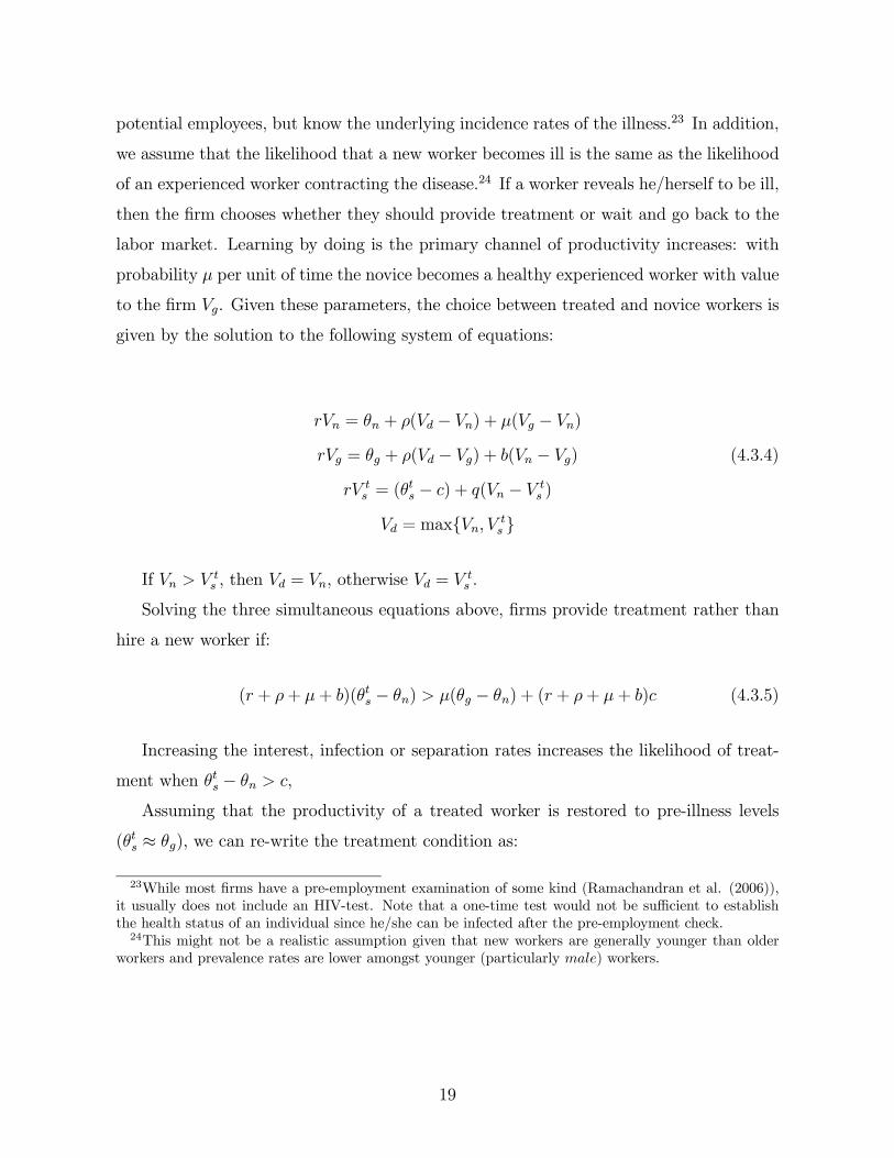
The second approach we employ characterizes monthly worker absenteeism due to
sickness around the time of ARV treatment onset. We use information provided by the
treatment program to define the month and year of treatment initiation of each enrolled
worker. Of the 449 workers (see Appendix Table 1) who were at some point on ARV’s,
94 enrolled in 2001, 84 in 2002, 51 in 2003, 64 in 2004, 115 in 2005 and 41 in 2006. Thus,
there is substantial variation in the timing of the initiation of ARV treatment.13
Our empirical strategy uses the variation resulting from the staggered timing of the
start of treatment as a way to estimate the patterns of absenteeism of HIV infected
workers around the time of ARV therapy inception. In our main specification we control
for month and person fixed effects and moreover we also include as controls a large sample
13We were able to match 441 of the 449 (98%) patients on ARVs to the HR database.
9

of workers from the company who are not associated with the program, which should help
us better account for other unobservable factors that might be slowly changing at the firm
level over time.
We estimate OLS regressions of the following form:
outcomept = β0 +Xi
αidist from treatmentipt + β1δp + β2τ t + ²pt , (2)
where outcomept is one of our dependent variables of interest (usually, duration of
absences due to sickness and/or ordinary leaves), measured in days for each month and
person cell. The variables dist from treatmenti are a set of dummy variables equal to
one if a person had started ARV therapy i months ago. We restrict i to be +/- 12 months
in the main specification but we also show graphical results that extend the time interval
to +/- 24 and +/- 36 months. We usually also control for person effects (δp) and month
effects (τ t).
The two empirical strategies are similar given that in both cases the source of variation
used comes from the timing of when people enroll in the ARV program. The fixed effects
model in the first strategy which only uses workers on ARV treatment, compares the
same person at up to three points in time (0, 6 and 12 months) and rescales the effect by
changes in the CD4 count from the first stage regression. The fixed effects model in the
second strategy estimates the reduced form patterns of absenteeism over a much longer
time window, but includes also absenteeism for healthy/never treated workers who only
help identify time effects.
There are two main reasons that these strategies do not identify the impact of ARV
treatment on absenteeism. Firstly, the decision to start treatment is certainly affected by
health (and potentially absenteeism) trends in the period immediately prior to treatment
start. In the program-evaluation literature, this source of bias is usually addressed by
modelling the selection process (e.g. Ashenfelter and Card, 1985). We have decided
against this approach since the estimation of the selection process generally requires an
exclusion restriction and in our particular case there are no plausible exclusion restrictions
across the selection into treatment and labor market outcome equations.
10

Secondly we do not have a reliable control group. In our model, the ”no treatment”
comparison group are esentially other HIV workers infected at a different time and workers
who were never enrolled in the program. As a result, our estimated effects are almost
certainly smaller than the “treatment effect of receiving ARV therapy”, given that in the
absence of treatment, many of the workers would have died. As previously mentioned, in
the absence of treatment, the median time between the development of AIDS and death
is 9.2 months (Morgan et al. 2002).
We run a number of alternative specifications in order to test the validity of our
results. We present figures based on non-parametric Fan locally weighted regressions to
show the pattern of absences before and after the introduction of ARV treatment. Since
some of our workers exit the sample due to death or separation from the company, in
our main unbalanced sample not all persons have data available for each month relative
to the starting date of treatment. Thus the number of persons identifying a particular
dist from treatmenti coefficient is not constant and these compositional changes could
give rise to possible trends in the data around the starting date. Therefore, we also
include results using a “balanced” panel of workers that have at least 12 (or 24, or 36)
months of post treatment data. Since the data from one of the mines (Jwaneng) extends
over a much longer time period, we can additionally use intervals that are 5 years before
and 4 years after the onset of ARV treatment. We also performed a number of additional
robustness checks: we re-ran our specification by splitting the sample by early vs. late
adopters, gender, worker band and mine. Except in the specifications that include person
fixed effects (where we use Huber-White standard errors), we cluster our standard errors
at the person level (Bertrand, Duflo and Mullainathan (2004)).
3.3 Accounting for Attrition
In this section we discuss the patterns of attrition in our data and describe the approach
that we take to correct for the potentially selective attrition of participants in the ARV
program. While selective attrition is a concern in all longitudinal datasets, it can be
particularly important in the present analysis since we are dealing with a population in
which death related attrition is expected to be important in light of the nature of the
disease that we study. In Figure 2 in the appendix we plot monthly attrition rates for
11

the first three years after the start of ARV therapy. The increase in overall attrition is
relatively linear over time and averages below 10% per year. The same graph also breaks
down the distribution of attrition due to death at the time of exit or regular separation
from the company. Roughly 60% of separations are due to death while working at the
company, although we cannot accurately measure mortality since the company does not
track former workers after they separate from the company.
We use three different sampling strategies in this analysis. The balanced sample in-
cludes only those individuals for whom we have labor supply information for all the
months between treatment start and sample window. The sample windows are 6 and
12 months for the health/CD4 sample and 12, 24 or 36 months for the regressions that
measure the pattern of absenteeism around ARV treatment start.14 The second sample is
unbalanced and includes all available monthly absenteeism observations for as long as the
individual is observed in the HR database. If selective attrition is severe, we expect the
results from the balanced and unbalanced sample to be different. The third approach ap-
plies the inverse probability weights (IPW) technique (Fitzgerald, Gottschalk and Moffitt
(1998) and Wooldridge (2002)) to adjust for selection bias due to observable characteris-
tics. Our approach will be to use background as well as absenteeism information at the
time of ARV treatment start to predict the probability (pi) that an individual i will still
be observed at the end of the sample period. This individual receives a weight equal to
1/pi in the regression analysis, therefore giving more weight in the regression to those
individuals whose observable characteristics predict higher attrition rates. The observ-
able characteristics used for this exercise are gender, age, worker band, date of treatment
start and absenteeism in the month prior to treatment start.15 This method, while useful,
cannot account for possible differential attrition due to unobserved characteristics. In the
absence of an exclusion restriction that would predict attrition due to health without a
direct impact on worker absenteeism, we will assume that attrition does not depend on
unobservables.16
14Additionally, we balance the data from the Jwaneng mine using a sample window of 5 years priorand 4 years after ARV treatment start.15While the background characteristics have little explanatory power, higher abseenteeism in the month
prior to treatment start has a positive impact on atrition (results not reported).16The concept of selection on observables in the context of attrittion is due to Fitzgerald, Gottschalk
and Moffitt (1998) and and is similar to the ”ignorability condition” (Wooldridge (2002)) or the concept
12

4 Results
4.1 CD4 counts and Worker Absenteeism
The relationship between CD4 count and worker absenteeism in the first year of
ARV treatment can be easily captured graphically. Figure 1 shows the pattern of the
two variables using non-parametric Fan locally weighted regressions with bootstrapped
standard errors clustered at the person level for both balanced and unbalanced samples.
For CD4 counts over 400 (employee is relatively healthy) there is little evidence of a
health-absenteeism link, although due to the limited amount of data, the estimates are
relatively imprecise. In the CD4 count range of 100-400, one can observe a clear increase in
absenteeism with deteriorating health and this effect is particularly strong for the sickest
employees with CD4 counts below 100. An employee with a CD4 count of 50 is absent
from work due to illness about a week a month.
Regression results of the effect of health measured by the CD4 count on worker absen-
teeism is provided in Table 1. Column (1) presents a simple OLS regression that shows
the existence of a correlation between health and labor market supply after we control
for a number of observable characteristics, such as age, gender, worker band and time
effects. These results are robust to the choice of sample (columns 3 and 4) or the in-
clusion of person fixed effects (column 2), which can only partly alleviate our concerns
about reverse causality or omitted variable bias. Next we turn to the analysis of our
preferred instrumental variable results. In Panel B of Table 1 we start by showing that
our two instrumental variables that indicate that the CD4 count was measured at 6 and
12 months after the start of therapy have a strong and statistically significant effect. On
average a person who gets on treatment has an increase in her/his CD4 count of 102
after 6 months and 127 after one year and this result is robust to the inclusion of person
fixed effects (column 6 of Panel B) or to different samples (columns 7 and 8 of Panel
B). The estimates using instrumental variables across specifications are large and highly
significant and vary between -.034 (standard error .004) and -.041 (standards error .005).
These estimates suggest that being on ARV therapy for 6 months, the average improve-
ments in health are equal to a CD4 count gain of 100 points and this causes illness-related
of ”missing at random” (Little and Rubin (1987)).
13

absenteeism to decrease by roughly 3.5 days per month, which is equivalent to a decrease
in the absenteeism rate by 16%. Two main conclusions can be drawn from an analysis of
Figure 1 and Table 1: (1) the overall impact of the health of an HIV infected individual
on worker absenteeism is economically large and (2) the effect is particularly strong for
those who are extremely sick (CD4 counts below 100).
4.2 Pattern of Absenteeism around ARV Treatment Start
A simpler way to depict the main results of the paper is to demonstrate the effect graph-
ically. Figure 2 plots the relationship between the average number of sickdays taken per
month and the distance from treatment start measured in months for a one year window.
Panel A uses a non-parametric Fan local regression model while the remaining three panels
come from regressions that contain worker and month fixed effects for the three sampling
strategies used. In all panels, one can observe a gradual increase in absenteeism in the
year before treatment starts. The increase in absenteeism is particularly steep in the six
months prior to therapy onset and peaks in the final month at roughly 5 days, which is
equivalent to an absenteeism rate of roughly 22%. The positive effects of treatment on
labor market outcomes is equally stark in the first months after the start of ARV therapy,
so that the shape of absences around treatment implementation is almost symmetric.
The corresponding regression results of illness-related worker absenteeism in the basic
equation (2) are in Table 2. Column (1), which uses an unbalanced sample and includes
only month fixed effects, presents estimates of αi, the coefficients for the treatment dum-
mies corresponding to a twelve month window around the onset of treatment. Compared
to workers who are not enrolled in the treatment program, workers with HIV/AIDS have
a higher duration of illness-related absenteeism (.484 days per month) even a year prior to
the start of treatment. The coefficients from this regression display the familiar inverse-V
patterns seen in the graphs, peaking at 5.13 days and then declining to less than a day
twelve months afterwards. Column (2) in the same table shows similar patterns from a
regression that also includes person fixed effects, where the omitted category (-11 month)
corresponds to one year prior to treatment start. The remaining columns show the same
regressions using the balanced and the inverse probability weight samples and the size
and significance of the results is very similar across specifications. In Table 3 we repeat
14

the analysis from Table 2 but we measure overall absenteeism, which includes sick and
regular leave spells. The same patterns emerge as previously and they suggest that en-
rolled (infected) workers do not use additional regular leave days during episodes of poor
health.
Next, we extend our analysis to wider intervals. Figure 3 and 4 repeat the graphs in
Figure 2 using two and three year windows, while Figure 5 which uses the longer data
series available from the Jwaneng mine plots illness-related absences 5 years prior and
4 years after ARV treatment start. These graphs confirm that most of the changes in
absenteeism occur within a one year window. The figures seem to suggest that workers
who are on treatment recover remarkably quickly and display very low rates of absenteeism
in the medium and long term (1-4 years post treatment initiation). Similarly, an HIV-
infected worker displays a pattern of labor supply that is similar to other “non-infected”
workers throughout a large part of the post-infection period, a finding that challenges
recent estimates in the literature (Fox et al. 2004).17 In Appendix Figure 3, we have
re-run our analysis with the longer intervals and data from the Jwaneng mine without
any person fixed effects: the coefficients outside the one year window are all small and
usually statistically indistinguishable from zero, suggesting that outside the short one
year window around treatment initiation, infected workers display similar labor market
outcomes (measured by absenteeism) to the other workers at the company who are not
enrolled in the treatment program.
Figure 6 shows how the patterns of absenteeism vary across different groups. In panel
A one observes that workers whose enrollment in the treatment program coincided with
the start of ARV treatment have higher absenteeism rates than workers who started
treatment after program enrollment. Similar patterns are evident in the next two panels,
where we observe that workers who are sicker at the time of ARV start, display higher
absenteeism rates in the year prior to treatment start. Panel B shows that ARV patients
who enrolled closer to the time of program start (2001-2002) have higher absenteeism
than those enrolling later (2003-2004). Also, in panel C we plot patients with low (<150)
and high (>150) CD4 counts at treatment start and not surprisingly, those with better
17One possible explanation for this finding is that stigma (in the absence of effective treatment) dis-courages workers from revealing their status so that infected workers are only observed very late in theirpost-infection period.
15

health are less likely to be absent. The last panel of Figure 6 shows no differences in
absenteeism between women and men.
In sum, given the unusual length of the absenteeism panel of almost 10 years and the
fact that Debswana’s ARV program was one of the first on the African continent, we were
able to map out the short, medium and long run patterns of absenteeism of HIV/AIDS
infected workers who receive ARV treatment. Our main conclusions are as follows: (1)
infected workers are as productive in terms of absenteeism for most of the period when
they are HIV positive, (2) about one year around the time of ARV treatment start, we see
a steep inverse-V pattern of absenteeism that peaks at about 5 days of absence a month,
and (3) in the period 1-3 years after treatment start, patterns of absenteeism are similar to
non-enrolled workers suggesting that ARV’s are extremely effective in improving workers
health and ability to work.
5 Is it Cost Effective for Firms to Provide ARVs?
Our discussion so far has established that to the extent that worker absenteeism is a good
proxy for productivity, ARVs are a successful way to restore the productivity of infected
workers. In this section, we present a simple model to analyze the cost and benefits
of treatment to firms. First, we show the conditions under which treatment of workers
with HIV/AIDS is preferred to non-treatment (without early termination) and secondly
we show the conditions under which a firm prefers to hire an inexperienced new worker
instead of providing treatment to an infected (and experienced) worker. In particular,
this framework models the recruitment problem facing a large number of firms in Sub
Saharan Africa that have to choose between providing/financing treatment of infected
workers with 5-15 years of experience or recruiting novices. Our model builds on the
rich literature, started by Becker (1964) and extended most recently by Acemoglu and
Pischke (1999), that has explored the rationale for why firms might provide a number of
human-capital enhancing investments to their workforce.
To motivate the firm’s choice we assume that firms are infinitely lived. There are three
types of workers: healthy workers, sick workers and inexperienced workers. The healthy
and sick workers are assumed to have considerably more experience than new recruits.
16

Using asset equations we can write down the value of each type of worker to the firm
taking into account the probability of separation between the worker and the firm.18
The value to the firm of a healthy experienced worker Vg is given by
rVg = (MPLg − wg) + ρ(Vd − Vg) + b(Vn − Vg) (4.3.1)
where r is the interest rate,MPLg and wg is the marginal product of labor and wage of
a healthy worker. We assume that the firm earns rents on a worker as a result of frictions
in the labor market that make the firm a wage setter (Burdett and Mortensen (1978),
Manning (2003), Postel-Vinay and Robin (2002)).19 A healthy worker has a probability
ρ of contracting a fatal, but treatable disease. If the worker becomes ill, the firm has a
choice of whether to keep the ill worker with no treatment, whether to provide treatment
to the worker or whether to replace the ill worker with a new worker. More formally, we
define Vd = max{V ts , V us , Vn}, where V ts is the value to the firm of an ill worker receiving
treatment, V us is the value to the firm of an untreated infected worker and Vn is the value
to the firm of a new recruit. We also include the possibility of non-illness related worker
turnover; with probability b per unit of time, a healthy worker will separate from the firm
in which case a firm hires a new worker.
To solve the firm’s problem, we start by establishing the conditions under which firms
will provide treatment conditional on worker infection. In particular, we compare the
value (to the firm) of providing treatment (or not) to a sick worker. We assume further
that firms bear the cost of treatment. In addition, we assume that treatment increases the
expected duration of employment with the firm. In particular the probability of illness-
related separation is lower under treatment q < δ.20 Following separation, the firm hires
a new worker of value Vn. Given these assumptions, the value to the firm of a sick worker
18We borrow the modelling of the firm’s problem from Shapiro and Stiglitz (1984). We abstract fromother human-capital enhancements that the firm might choose to provide such as training. In our simpleframework, productivity increases through the process of learning-by-doing.19Labor market imperfections are likely to be more relevant in developing country settings (see Agenor,
1995 for a detailed review)20This assumption follows from the fact that the treatment is effective and reduces mortality/morbidity
risk and that treatment can only be obtained while in employment. The latter is typical of most firm-based treatment programs.
17

with treatment V ts , and without treatment Vus is given by
21:
rV ts = (MPLts − ws − c) + q(Vn − V ts ) (4.3.2)
rV us = (MPLus − ws) + δ(Vn − V us )
The firm decides to provide treatment if V ts − V us > 0. It is convenient to write the
net instantaneous payoff to the firm (MPLts − ws), and (MPLus − ws) as θts and θts. The
treatment condition can be stated as follows:
(q + r)(θts − θus ) + (δ − q)(θts − rVn) > (δ + r)c (4.3.3)
There are two parts to the left hand side of the treatment condition. Firstly, the
net benefit of treatment includes a productivity difference captured by θts − θus > 0.22
Secondly, providing treatment keeps a more productive worker longer and obviates the
need for a new worker. The sum of these two terms is compared to the cost of treatment
c.
This treatment condition illustrates that firms will have larger incentives to offer treat-
ment to some types of workers over others. In particular, workers for whom the costs of
illness (in terms of foregone productivity) are very high relative to treatment or workers
for whom the returns to tenure are very high are more likely to satisfy the treatment
condition. Alternatively, if separation rates of sick workers, captured by δ, is very high,
firms are more likely to provide treatment if and only if (θts−rVn) is greater than the costof treatment, c.
To complete the model we need to determine the firm’s choice between hiring a new
worker or providing treatment when treatment is preferred to non-treatment. In this
direction, we compare the value to the firm of a new worker relative to a treated worker.
We assume that firms do not have any information regarding the health status of
21We assume that the wage paid to a treated and untreated ill worker is the same ws.22We assume that healthy and unhealthy workers with the same characteristics earn the same wages.
Differences in θts− θus are therefore driven by differences in productivity induced by treatment efficacy.
18
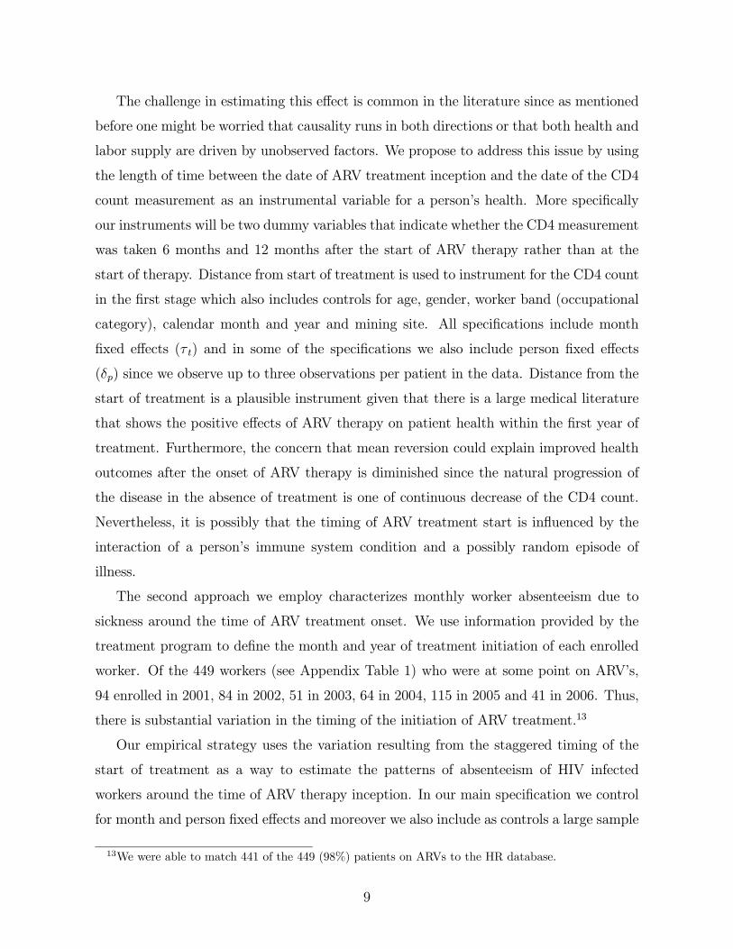
potential employees, but know the underlying incidence rates of the illness.23 In addition,
we assume that the likelihood that a new worker becomes ill is the same as the likelihood
of an experienced worker contracting the disease.24 If a worker reveals he/herself to be ill,
then the firm chooses whether they should provide treatment or wait and go back to the
labor market. Learning by doing is the primary channel of productivity increases: with
probability µ per unit of time the novice becomes a healthy experienced worker with value
to the firm Vg. Given these parameters, the choice between treated and novice workers is
given by the solution to the following system of equations:
rVn = θn + ρ(Vd − Vn) + µ(Vg − Vn)
rVg = θg + ρ(Vd − Vg) + b(Vn − Vg) (4.3.4)
rV ts = (θts − c) + q(Vn − V ts )
Vd = max{Vn, V ts }
If Vn > Vts , then Vd = Vn, otherwise Vd = V
ts .
Solving the three simultaneous equations above, firms provide treatment rather than
hire a new worker if:
(r + ρ+ µ+ b)(θts − θn) > µ(θg − θn) + (r + ρ+ µ+ b)c (4.3.5)
Increasing the interest, infection or separation rates increases the likelihood of treat-
ment when θts − θn > c,
Assuming that the productivity of a treated worker is restored to pre-illness levels
(θts ≈ θg), we can re-write the treatment condition as:
23While most firms have a pre-employment examination of some kind (Ramachandran et al. (2006)),it usually does not include an HIV-test. Note that a one-time test would not be sufficient to establishthe health status of an individual since he/she can be infected after the pre-employment check.24This might not be a realistic assumption given that new workers are generally younger than older
workers and prevalence rates are lower amongst younger (particularly male) workers.
19

c∗ =r + b+ ρ
r + b+ ρ+ µ(θts − θn) (4.3.6)
The treatment condition above provides useful intuition: firms compare the net benefit
of treatment against the cost of treatment and the foregone opportunity of a new worker
becoming a healthy and productive worker. The magnitude of (θts − θn) depends on the
differential slopes of the marginal product of labor and wage profiles for a given worker
over his/her tenure in the firm. In order for firm-based provision of ARVs to be optimal,
two conditions need to be satisfied. Firstly, we require that there is a wedge between the
marginal product of labor and worker wages. Theoretically this wedge has been posited
in different types of models, such as the presence of labor market imperfections (Burdett
and Mortensen (1998), in competitive implicit contract models such as (Lazear, 1979)
or in models with symmetric imperfect information (Harris and Holmstrom, 1982). The
second condition needed for the provision of ARVs by the firm is driven by the size of
differential rents to the firm of “experienced” but ill workers relative to “novice” workers
of unknown health status. In order for the right hand side of equation 4.3.6 to be positive,
we require that the marginal product-wage gap be larger for workers with longer tenure.
The empirical literature on the profile of productivity and wages with tenure is incon-
clusive. A number of microeconomic studies have examined the tenure-productivity and
tenure-wage relationship.25 Two recent contributions, Hellerstein, Neumark and Troske
(1999) and Crepon, Deniau and Perez-Duarte (2003), attempt to estimate the relative
marginal productivity of different types of labor. Hellerstein et. al. (1999) using US
data conclude that the marginal productivity of middle aged workers rises at the same
rate as earnings. Conversely Crepon et. al.(2003) using French data find that earnings
rise faster than productivity for middle-aged workers, suggesting a declining marginal
productivity-wage gap with tenure.26 The findings in these studies suggest that firms
would not provide treatment in equilibrium since θts − θn ≤ 0. Thus hiring a new worker
25These include papers by Lazear (1979, 1981), Medoff and Abraham (XXXX), Hutchens (1987, 1989),Carmichael (1983), Jovanovic (1981), Borjas (1981) and Jovanovic and Mincer (1947).26An earlier paper by Kotlikoff and Gokhale (1992) using earnings data from a Fortune 500 company
arrives at the same conclusion.
20

dominates treating a long-tenure infected worker, a result consistent with a conjecture by
Rosen (2006) that the economic basis for firm-based treatment provision is thin.
However, two recent cross-country studies show that countries or sectors with a high
proportion of long tenure workers have higher productivity (Auer, Berg and Coulibaly
(2004)) and that economies with a larger share of 40-49 year olds have higher growth
rates (Feyrer 2007). While omitted variables are likely to compromise the validity of
these conclusions, these results suggest an alternative production function with stronger
complementarities than those assumed by the micro-studies. In particular, firms might
care about maintaining a substantial share of long tenure workers, since the marginal
productivity of any worker is likely to depend on the average tenure of the workforce.
In a world of stronger complementarities, firm-based treatment provision to experienced
workers could be optimal.
Assuming that θts − θn ≥ 0, we turn to the data to find reasonable measures of
each of the parameters above to establish the conditions under which firms will offer
their workers treatment. We assume a discount rate r = 0.08. Firm data from the
South Africa Manufacturing survey yields an average tenure of 7 years which implies that
b = 0.14 (South Africa Investment Climate Report (2004)). Our HIV incidence data
comes from Shelton (2006). We take as our estimate of ρ, the high end of his estimates
of HIV incidence rates over a duration of one year: ρ = 0.06. Our estimate of µ depends
on the share of individuals who would be revealed to be high-productivity types in time
interval t. We assume that 12% of new workers reach high productivity levels in their
first year. This implies that µ = (1− ρ) (1− b) ∗ 0.12 = 0.1.27
Generating estimates for the magnitude of (θg − θn) is not straightforward given the
discrepancies in the literature and limited empirical estimates. Postel-Vinay and Robin
(2002) is the only paper with usable estimates for this calibration. We make the following
assumptions regarding the size of θts − θn : a new worker is analogous to the typical
worker in the 25th percentile and an experienced worker is in the 75th percentile in
27Substituting for these parameters in our treatment condition
c∗ = 0.736 ∗ (θg − θn)
The slope parameter 0.736 is sensitive to the size of µ. For µ = 0.3, the slope is now 0.48 and 0.36when µ = 0.5.
21

the distribution of firm quality. Using results from Postel-Vinay and Robin (2002) for
unskilled workers suggests that, (θg − θn) ≈ 0.43w. Assuming that the experienced
worker comes from the median firm reduces this magnitude to 0.33w.28 Using these
estimates, together with median wages from recent manufacturing surveys, we calculate
the percentage of treatment costs that firms are willing to pay. We assume that the cost of
treating a worker is uniform across the central and eastern African countries at $360/year
or $30/month. The monthly cost of treatment in Botswana, Namibia and Swaziland is
estimated at $100 and $141 in South Africa.29 The results of this calibration are shown
in figure 7. We show the results for two levels of the productivity-wage gap and two
assumptions about the efficacy of treatment. The first bar shows the percent the typical
firm is willing to pay when we assume that the productivity wedge (θg − θn) = 0.1w
and the effect of treatment fully restores productivity. The second column maintains the
size of the wedge but assumes that treatment only partially restores worker productivity
so that the wedge gap is 0.7 ∗ (θg − θn) . The third and fourth bars show corresponding
numbers when the size of the productivity-wage gap is 0.4w. Median monthly wages of an
unskilled worker range between $79/month in Eritrea to $136 in Nigeria. For the Southern
African economies, wage estimates are only available for production workers (both skilled
and unskilled). The median monthly estimates range from $156 in Botswana to $702 in
South Africa (various publications, World Bank).
Assuming that (θg − θn) ≈ 0.1w and that treatment fully restores productivity, thetypical firm in Tanzania can finance 13% of the cost of providing treatment for an unskilled
worker, while the typical firm in Nigeria can finance about 33% of the cost of treatment.
In the Southern African economies where the costs of treatment are higher, the typical
firm in Botswana can finance about 11% of treatment costs while the typical firm in
South Africa can finance about 36% of treatment costs. 30 Assuming that treatment only
28These numbers come from figure 1 in Postel-Vinay and Robin(2002). In order to generate aproductivity-wage gap that is a function of a particular wage, we convert wages at the 25th and 75thpercentiles as functions of the median wage.29These numbers are based on costs of the AMPATH treatment program in Kenya. The breakdown
is about $150 for first line ARV drugs and $200 are the remaining treatment related costs (such clinic,medical and lab expenditures). The Botswana estimate is derived from Debswana’s per patient costs.The estimate for South Africa comes from Cleary, McIntyre and Boulle (2006).30Note that we assume uniform labor market frictions across economies and even more unrealistically
uniform productivity-wage gaps across countries.
22

restores productivity to 70% of pre-infection productivity, firms in Nigeria and South
Africa can finance about 25% of treatment costs. Assuming a productivity-wage gap
of 0.4w implies that the typical firm in Tanzania could finance 52% of treatment costs,
while a corresponding firm in Botswana can finance 46% of treatment costs for all of its
workers. Assuming less than perfect efficacy of treatment the typical firm in Nigeria and
South Africa can finance 94% and 100% of treatment costs. Taking (θg − θn) ≈ 0.1w
as the most plausible productivity-wage gap, manufacturing firms in Africa can finance
between 10-25% of the costs of ARV treatment when treatment is less than perfect and
13-33% when treatment efficacy fully restores worker productivity. The benefits to firms
of providing ARV treatment is large considering that the socio-economic benefits from
ARV treatment extend well beyond labor supply. As an example, Graff Zivin et al. (2006)
show large gains to the health and schooling of children in households with adults receiving
treatment.
6 Conclusion
In this paper we exploit an unusually long panel dataset of worker absenteeism from
the Debswana Diamond Company as well as information on one of Africa’s first firm-based
ARV treatment programs to understand the effect of HIV/AIDS and ARV treatment
on worker productivity. We find evidence that compared to other workers at the firm,
individuals who are infected with HIV/AIDS display similar patterns of absenteeism until
roughly one year prior to treatment start, when absenteeism starts to increase sharply.
From an absenteeism peak of 5 days in the month of treatment onset, the workers quickly
recover within the first year of treatment and then continue for the next three years to
have patterns of absenteeism that are similar to those of healthy workers. Our results
suggest that in an African context, ARV’s are effective in the short, medium and long
run in improving the health and productivity of workers and challenge recent claims that
global support of ARV treatment will create health pensioners (The Economist. August
2006).
In the final section of the paper, we build a simple model in order to understand when
the free provision of treatment to HIV workers is beneficial to firms. We first show that
23

the decision to provide treatment to an experienced sick worker depends crucially on the
assumption that the marginal product-wage gap be larger for workers with longer tenure
than newly hired inexperienced workers. Next we review the empirical literature on the
pattern of worker productivity and wages with tenure and conclude that the micro and
macro based studies do not yield any conclusive conclusions. Using a plausible positive
measure of the marginal product-wage gap and data from manufacturing firm surveys
in Africa, we show that firms can recover between 10-33% of treatment costs. These
results do not account for other possible benefits of ARV treatment to the firm, such as
reductions in medical and health insurance costs, death benefits, funeral costs as well as
the benefits to the firm’s reputation from investing in socially responsible programs.
Since the cost of treatment exceeds the benefits of treatment across a range of economies
in Eastern and Southern Africa, widespread firm-based ARV provision is an unlikely pol-
icy option. And while relatively recent developments, such as the creation of the Global
Business Coalition on HIV/AIDS, foreshadow an increasing involvement of firms in com-
bating HIV/AIDS, the majority of firms in the developing world that have established
workplace programs for their employees are very special companies, similar to the case
of Debswana in Botswana. However, since our results suggest that the private bene-
fits to firms from treatment can be significant, the provision of public subsidies to ARV
treatment programs administered by private companies has the potential to become an
important mechanism to provide treatment to people affected by HIV/AIDS in a re-
source constrained setting like Africa, as exemplified by the success of the public-private
partnership between DaimlerCrysler and GTZ in South Africa.
24

References
Acemoglu, Daron and Simon Johnson, (2006). ”Disease and Development: The Effect
of Life Expectancy on Economic Growth,” NBER Working Papers 12269, National
Bureau of Economic Research, Inc.
Acemoglu, Daron., and Jorn-Steffen Pischke (1999) “Beyond Becker: Training in Im-
perfect Labor Markets” Economic Journal 109: 112-142
Auer, Peter and Janine Berg and Ibrahim Coulibaly, 2004. “Is a stable workforce good
for the economy? Insights into the tenure-productivity-employment relationship,” Em-
ployment strategy papers 2004-15, International Labour Office.
Becker, Gary (1964) Human capital. Chicago: The University of Chicago Press
Bell, Clive, Shanta Devarajan and Gersbach, H. 2003. “The Long Run Economic Costs
of AIDS. Theory and an Application to South Africa.” Policy Research Working Paper
3518, World Bank, Washington, D.C.
Bertrand Marianne and Esther Duflo and Sendhil Mullainathan, 2004. “How Much
Should We Trust Differences-in-Differences Estimates?,” The Quarterly Journal of Eco-
nomics, MIT Press, 119(1) 249-275
Burdett, Kenneth and Mortensen, Dale, 1978. “Labor Supply Under Uncertainty”. In
Research in Labor Economics, ed. Ronald G. Ehrenberg. Greenwhich, CT: JAI Press.
. 1998. “Wage Differentials, Employer Size, and Unemployment”. Interna-
tional Economic Review 39 (2): 257-73.
Canning, David, 2006, “The Economics of HIV/AIDS in Low-Income Countries: The
Case for Prevention”, The Journal of Economic Perspectives 20(3)
Case, Anne and Angus Deaton, (2006) “Health and wellbeing in Udaipur and South
Africa”, Center for Health and Wellbeing, Princeton University, WP
Cleary S, McIntyre D, Boulle A. 2006. “The cost-effectiveness of Antiretroviral Treat-
ment in Khayelitsha, South Africa — a primary data analysis”, Cost Effectiveness and
Resource Allocation. Vol. 4:20
25

Crepon, B., Deniau, N., and Perez-Duarte, S. 2002. “Wages, Productivity and Worker
Characteristics” Institut National De La Statistique et des Etudes Economiques (IN-
SEE) WP #2003-04.
Duggan, Mark and William N. Evans, 2005. “Estimating the Impact of Medical Innova-
tion: A Case Study of HIV Antiretroviral Treatments,” NBER Working Papers 11109,
National Bureau of Economic Research, Inc.
Feyrer, James, (2007) “Demographics and Productivity”, forthcoming in Review of
Economics and Statistics
Fitzgerald, John, and Peter Gottschalk and Robert Moffitt, (1998). “An Analysis of the
Impact of Sample Attrition on the Second Generation of Respondents in the Michigan
Panel Study of Income Dynamics”. Journal of Human Resources, Spring 1998
Floridia, M., et al., 2002. “HIV-Related Morbidity and Mortality in Patients Starting
Protease Inhibitors in Very Advanced HIV Disease”, HIV Medicine, 3(2): 75-84.
Fox MP and Rosen S and MacLeod WB et al. (2004) “The impact of HIV/AIDS on
labour productivity in Kenya”. Tropical Medicine and International Health 9: 318-324.
Graff Zivin, Joshua and Harsha Thirumurthy and Markus Goldstein, 2006. “AIDS
Treatment and Intrahousehold Resource Allocations: Children’s Nutrition and School-
ing in Kenya,” NBER Working Papers 12689, National Bureau of Economic Research,
Inc.
Hammer, S.M., et al., 1997. “A Controlled Trial of Two Nucleoside Analogues Plus In-
dinavir in Persons with Human Immunodeficiency Virus Infection and CD4 Cell Counts
of 200 per Cubic Millimeter or Less”, The New England Journal of Medicine 337(11):
725-33.
Harris, Milton and Holmstrom, Bengt. 1982. “A Theory of Wage Dynamics”. Review
of Economic Studies July 49 : 315-33
Hellerstein, Judith K and Neumark, David and Troske, Kenneth R, 1999. “Wages, Pro-
ductivity, andWorker Characteristics: Evidence from Plant-Level Production Functions
26

and Wage Equations,” Journal of Labor Economics, University of Chicago Press, 17(3):
409-46
Kalemli-Ozcan, Sebnem (2006), “AIDS, Reversal of the Demographic Transition and
Economic Development: Evidence from Africa,” NBER Working Paper 12181
Kaufmann GR, Bloch M, Finlayson R, et al. (2002). “The extent of HIV-1-
relatedimmunodeficiency and age predict the long-term CD4 T lymphocyte response to
potent antiretroviral therapy.” AIDS. 16:367.
Koenig, Serena P., Fernet Leandre, and Paul E. Farmer. 2004. “Scaling-up HIV Treat-
ment Programmes in Resource-limited Settings: The Rural Haiti Experience”. AIDS
18:S21-S25
Lazear, Edward. 1979. “Why is there Mandatory Retirement?” Journal of Political
Economy 87(6) : 1261-84.
Little, R and D Rubin. 1987. Statistical Analysis with Missing Data, New York, Wiley.
Manning, Alan. 2003. Monopsony in Motion. Princeton University Press, Princeton
New Jersey.
Marins, Jose Ricardo P. et al. 2003. “Dramatic Improvement in Survival Among Adult
Brazilian AIDS patients.” AIDS 17:1675-1682.
Mbakile, Bekezela (2005). Presentation given at the Center for Global Development,
October 2005
Morgan, Dilys et al. 2002. “HIV-1 Infection in Rural Africa: Is There a Difference in
Median Time to AIDS and Survival Compared With That in Industrialized Countries?”
AIDS 16:597-603.
Postel-Vinay, Fabien and Jean-Marc Robin, (2002). “EquilibriumWage Dispersion with
Worker and Employer Heterogeneity,” Econometrica, Econometric Society, 70(6):2295-
2350
27

Ramachandran. Vijaya and Manju Kedia Shah and Ginger Turner, (2006). “Does the
Private Sector Care About AIDS? Evidence from Investment Climate Surveys in East
Africa,” Working Papers 76, Center for Global Development.
Rosen, Sydney. 2006. quoted in Financial Times, December 1 2006.
Rosen, Sydney, Rich Feeley, Patrick Connelly and Jonathan Simon, (2006), ”The private
Sector and HIV/AIDS in Africa: Taking Stock of Six Years of Applied Research,”
Center for International Health and Development Discussion Paper No.7, 2006.
Sachs, Jeffrey, (2003). ”Institutions Don’t Rule: Direct Effects of Geography on Per
Capita Income,” NBER Working Papers 9490, National Bureau of Economic Research,
Inc.
Shapiro, Carl and Joseph E. Stiglitz (1984), “Equilibrium Unemployment as a Worker
Discipline Device”, American Economic Review, (74): 433-444.
Shelton, JD, Halperin DT, and Wilson, D. “Has global HIV incidence peaked?”, Lancet
367 : 1120—1122.
Strauss, John and Duncan Thomas (1998). “Health, Nutrition, and Economic Devel-
opment”. Journal of Economic Literature 36: 766-817
Thirumurthy, Harsha and Johsua Graff-Zivin and Markus Goldstein, 2005. “The Eco-
nomic Impact of AIDS Treatment: Labor Supply in Western Kenya,” NBER Working
Papers 11871, National Bureau of Economic Research, Inc.
Thomas, Duncan et al (2006). “Causal Effect of Health on Labor Market Outcomes:
Experimental Evidence” UCLA mimeo
UNAIDS. (2002). “The Private Sector Responds to the Epidemic: Debswana -a Global
Benchmark. Geneva: Joint United Nations Program on HIV/AIDS (UNAIDS Case
Study)
The Economist. “Look to the Future: The War Against AIDS”. August 19th 2006. The
Economist Newspapers Ltd. London, UK.
28

UNAIDS. (2006). Report on the global AIDS epidemic 2006. Geneva: Joint United
Nations Program on HIV/AIDS (UNAIDS)
Wooldridge, Jeffrey, (2002). “Inverse probability weighted M-estimators for sample se-
lection, attrition and stratification,” CeMMAP working papers CWP11/02, Centre for
Microdata Methods and Practice, Institute for Fiscal Studies.
Wools-Kaloustian, Kara, et al. 2006. “Viability and Effectiveness of Large-scale HIV
Treatment Initiatives in Sub-Saharan Africa: Experience from Western Kenya. AIDS
20(1): 41-48
World Bank. 2003. “Uganda: An Assessment of the Investment Climate”. Washington
DC: World Bank
World Bank. 2004. “Tanzania: An Assessment of the Investment Climate”. Washington
DC: World Bank
World Bank. 2004. “Kenya: An Assessment of the Investment Climate”. Washington
DC: World Bank.
World Bank. 2005. “South Africa: An Assessment of the Investment Climate”. Wash-
ington DC: World Bank.
Young, Alwyn, (2005) “The Gift of the Dying: The Tragedy of AIDS and the Welfare
of Future African Generations”, Quarterly Journal of Economics Vol 120 No. 2
29

Figure 1: Relationship between CD4 Count and Sick Days from Work
Note: Non-parametric Fan locally weighted regression with bootstrapped standard errors clustered by worker. Sickness-related absence duration data comes from the company's HR database and was linked to the CD4 count measured at the start of ARV treatment as well as 6 and 12 months after treatment start. Panel A uses an unbalanced sample while Panel B uses a balanced sample that includes only patients with three CD4 mesures.
05
10D
ays
abse
nt p
er m
onth
0 100 200 300 400 500 600CD4 count
Panel B: Balanced Panel
05
10D
ays
abse
nt p
er m
onth
0 100 200 300 400 500 600CD4 count
Panel A: Unbalanced Panel

Note: Panels A is from a Non-parametric Fan locally weighted regression with bootstrapped standard errors clustered by worker. Panels B, C and D are from a fixed effect regression that includes worker and month fixed effects and they corresponds to the results in Columns 2, 4 and 6 of Table 2. Sickness-related absence duration data comes from the company's HR database. The interval used is one year before and after the onset of ARV treatment. Panels A and B use an unbalanced sample as defined in Table 2, panel C a balanced sample and panel D a sample with weights based on inverse probability weights (IPW).
02
46
Day
s ab
sent
per
mon
th
-12 0 12Months before treatment
Panel A: non-parametric
02
46
Day
s ab
sent
per
mon
th-12 0 12
Months before treatment
Panel B: unbalanced sample0
24
6D
ays
abse
nt p
er m
onth
-12 0 12Months before treatment
Panel C: balanced sample
02
46
Day
s ab
sent
per
mon
th
-12 0 12Months before treatment
Panel D: ipw sample
Figure 2 : Effect of ARV treatment - One year window

Note: Panels A is from a Non-parametric Fan locally weighted regression with bootstrapped standard errors clustered by worker. Panels B, C and D are from a fixed effect regression that includes worker and month fixed effects and they corresponds to the results in Columns 2, 4 and 6 of Table 2. Sickness-related absence duration data comes from the company's HR database. The interval used is two years before and after the onset of ARV treatment. Panels A and B use an unbalanced sample as defined in Table 2, panel C a balanced sample and panel D a sample with weights based on inverse probability weights (IPW).
02
46
Day
s ab
sent
per
mon
th
-24 -12 0 12 24Months before treatment
Panel A: non-parametric
02
46
Day
s ab
sent
per
mon
th-24 -12 0 12 24
Months before treatment
Panel B: unbalanced sample0
24
6D
ays
abse
nt p
er m
onth
-24 -12 0 12 24Months before treatment
Panel C: balanced sample
02
46
Day
s ab
sent
per
mon
th
-24 -12 0 12 24Months before treatment
Panel D: ipw sample
Figure 3 : Effect of ARV treatment - Two year window

Note: Panels A is from a Non-parametric Fan locally weighted regression with bootstrapped standard errors clustered by worker. Panels B, C and D are from a fixed effect regression that includes worker and month fixed effects and they corresponds to the results in Columns 2, 4 and 6 of Table 2. Sickness-related absence duration data comes from the company's HR database. The interval used is two years before and after the onset of ARV treatment. Panels A and B use an unbalanced sample as defined in Table 2, panel C a balanced sample and panel D a sample with weights based on inverse probability weights (IPW).
02
46
Day
s ab
sent
per
mon
th
-36 -24 -12 0 12 24 36Months before treatment
Panel A: non-parametric
02
46
Day
s ab
sent
per
mon
th-36 -24 -12 0 12 24 36
Months before treatment
Panel B: unbalanced sample
02
46
Day
s ab
sent
per
mon
th
-36 -24 -12 0 12 24 36Months before treatment
Panel C: balanced sample
02
46
Day
s ab
sent
per
mon
th
-36 -24 -12 0 12 24 36Months before treatment
Panel D: ipw sample
Figure 4 : Effect of ARV treatment - Three year window

Note: Panels A is from a Non-parametric Fan locally weighted regression with bootstrapped standard errors clustered by worker. Panels B, C and D are from a fixed effect regression that includes worker and month fixed effects and they corresponds to the results in Columns 2, 4 and 6 of Table 2. Sickness-related absence duration data comes from the company's HR database for the Jwaneng mine. The intervals used are 5 years before and 4 years after the onset of ARV treatment. Panels A and B use an unbalanced sample as defined in Table 2, panel C a balanced sample and panel D a sample with weights based on inverse probability weights (IPW).
02
46
Day
s ab
sent
per
mon
th
-60 -24 -12 0 12 24 48Months before treatment
Panel A: non-parametric
02
46
Day
s ab
sent
per
mon
th-60 -24 -12 0 12 24 48
Months before treatment
Panel B: unbalanced sample
02
46
Day
s ab
sent
per
mon
th
-60 -24 -12 0 12 24 48Months before treatment
Panel C: balanced sample
02
46
Day
s ab
sent
per
mon
th
-60 -24 -12 0 12 24 48Months before treatment
Panel D: ipw sample
Figure 5 : Effect of ARV treatment - Jwaneng mine

Note: All panels are based on Non-parametric Fan locally weighted regression with bootstrapped standard errors clustered by worker. Sickness-related absence duration data comes from the company's HR database for. The intervals used are 2 years before and after the onset of ARV treatment and uses a unbalanced sample as defined in Table 2. Panel A plots outcomes for individuals who started on ARVs when they enrolled in the program (black, continuous line) versus those who started ARVs after enrollment (red, dotted line). Panel B plot those who enrolled early (2001-2002) in the program (black, continuous line) versus late (2003-2004) (red, dotted line). Panel C plots those with low CD4 at ARV start (<150) (black, continuous line) versus high CD4 count (>150)(red, dotted line). Panel D plots outcomes for men (black, continuous line) versus women (red, dotted line).
02
46
Day
s ab
sent
per
mon
th
-24 -12 0 12 24Months before treatment
Panel A: ARV at enrollment
02
46
Day
s ab
sent
per
mon
th-24 -12 0 12 24
Months before treatment
Panel B: Early versus Late
02
46
Day
s ab
sent
per
mon
th
-24 -12 0 12 24Months before treatment
Panel C: Low CD4 vs. High CD4
02
46
Day
s ab
sent
per
mon
th
-24 -12 0 12 24Months before treatment
Panel D: Men versus Women
Figure 6 : Effect of ARV treatment across groups

Notes: See Section 5 for a discussion of the assumptions made for the present calculations.
Figure 7: % Firm Coverage of Patient Treatment Cost
13.1 15.217.9 19.5
27.1
33 .5
11.513 .9
22 .0
36 .7
0
20
40
60
80
100
120
140
160
Tanza
nia
Eritrea
Ugand
a
Zambia
Kenya
Nigeria
Botswan
a
Swazila
nd
Namibi
a
South
Africa
% o
f mon
thly
trea
tmen
t cos
t
Baseline Coverage LessProductive
Wedge40%_base Wedge40%LessProductive
Appendix Figure 1: Timing of ARV enrollment
020406080
100120140
2001 2002 2003 2004 2005 2006
Year
Num
ber o
f w
orke
rs
Source: Author's calculations based on HR and ART program data.
Source: Author's calculations based on HR and ART program data.
Appendix Figure 2: Attrition since start of ARV's
0
0.05
0.1
0.15
0.2
0.25
0.3
0 5 10 15 20 25 30 35
Months since start of ARV's
Attr
ition
rate
attrition
death relatedattrition
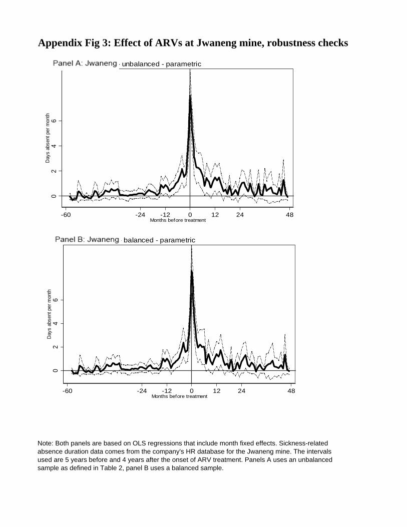
Appendix Fig 3: Effect of ARVs at Jwaneng mine, robustness checks
Note: Both panels are based on OLS regressions that include month fixed effects. Sickness-related absence duration data comes from the company's HR database for the Jwaneng mine. The intervals used are 5 years before and 4 years after the onset of ARV treatment. Panels A uses an unbalanced sample as defined in Table 2, panel B uses a balanced sample.
02
46
Day
s ab
sent
per
mon
th
-60 -24 -12 0 12 24 48Months before treatment
Panel B: Mine A - unbalanced - parametric0
24
6D
ays
abse
nt p
er m
onth
-60 -24 -12 0 12 24 48Months before treatment
Panel B: Mine A - balanced - parametric

Table 1: CD4 Counts and Absenteeism from Work
Panel A: Number of Sick Days per MonthOLS Fixed Effects OLS OLS IV IV-Fixed Effects IV IV
unbalanced unbalanced balanced ip-weights unbalanced unbalanced balanced ip-weights(1) (2) (3) (4) (5) (6) (7) (8)
CD4 count -0.011*** -0.011*** -0.007*** -0.010*** -0.041*** -0.034*** -0.037*** -0.040***[0.002] [0.002] [0.002] [0.002] [0.005] [0.004] [0.007] [0.006]
Mean of dep. variable 3.22 3.22 2.16 2.39 3.22 3.22 2.16 2.39
Panel B: First Stage for CD4 Count6 month dummy 101.738*** 108.876*** 107.674*** 89.030***
[10.653] [9.712] [12.669] [10.880]12 month dummy 126.925*** 127.155*** 130.188*** 113.538***
[12.224] [10.834] [13.945] [12.412]Mean of dep. variable 220.89 220.89 245.58 234.68F-test 70.91 95.62 50.94 52.36
Observations 845 845 414 844 845 845 414 844
Notes: Sick days from work data comes from the company's HR database and was linked to the CD4 count measured at the start of ARV treatment as well as 6 and 12months after treatment start. All regressions except in columns (2) and (6) include controls for age, worker band, gender and month and year of treatment start and thestandard errors are clustered at the person level. Results in columns (2) and (6) are based person fixed effects regressions. The instruments used in column (5)-(8) are twodummy variable indicators that indicate that the CD4 count was measured at 6 and 12 months after the start of ARV theraphy. The regressions in columns (3) and (7) use abalanced sample that includes only patients with three CD4 mesures. The regressions in columns (4) and (8) use inverse probability weights (IPW), and the remainingcolumns use an unbalanced sample.*** significant at 1% level. ** significant at 5% level. * significant at 10% level.
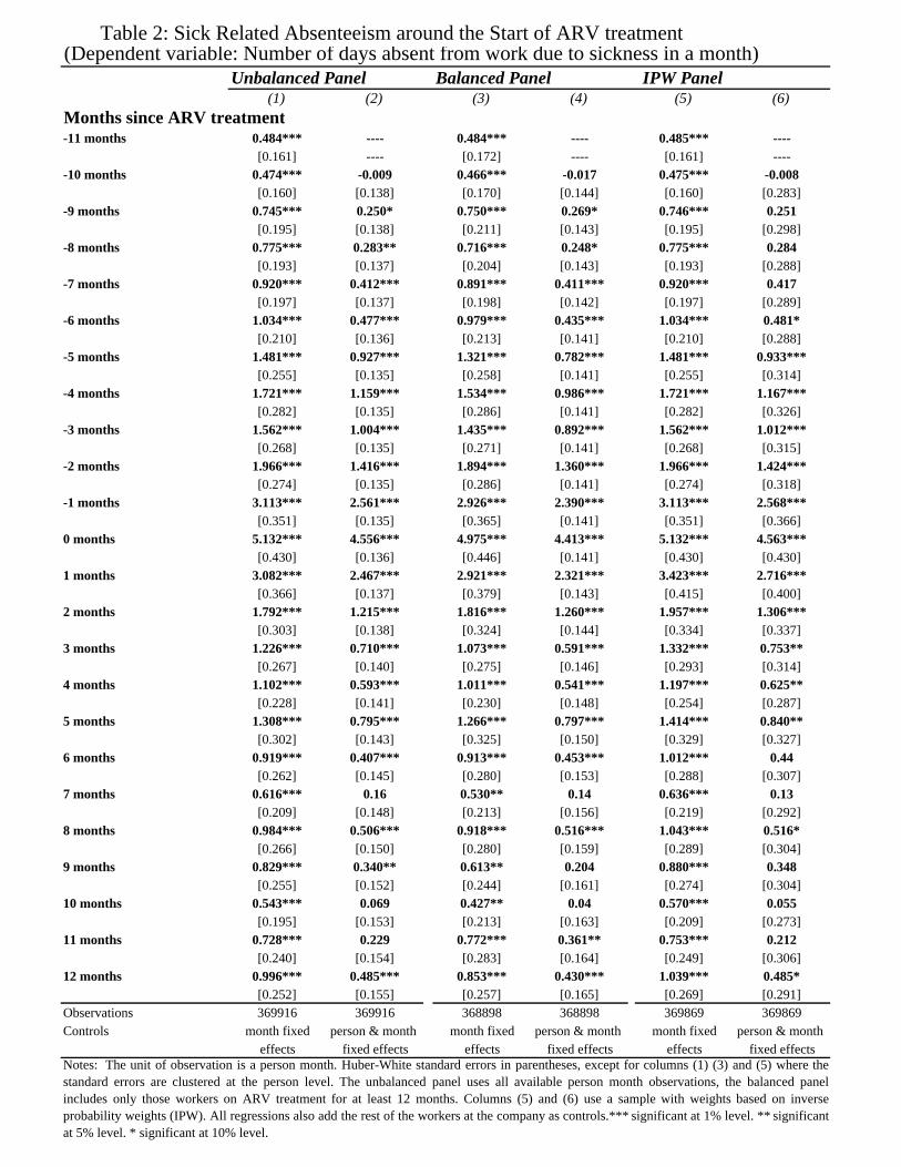
Table 2: Sick Related Absenteeism around the Start of ARV treatment(Dependent variable: Number of days absent from work due to sickness in a month)
Unbalanced Panel Balanced Panel IPW Panel(1) (2) (3) (4) (5) (6)
Months since ARV treatment-11 months 0.484*** ---- 0.484*** ---- 0.485*** ----
[0.161] ---- [0.172] ---- [0.161] -----10 months 0.474*** -0.009 0.466*** -0.017 0.475*** -0.008
[0.160] [0.138] [0.170] [0.144] [0.160] [0.283]-9 months 0.745*** 0.250* 0.750*** 0.269* 0.746*** 0.251
[0.195] [0.138] [0.211] [0.143] [0.195] [0.298]-8 months 0.775*** 0.283** 0.716*** 0.248* 0.775*** 0.284
[0.193] [0.137] [0.204] [0.143] [0.193] [0.288]-7 months 0.920*** 0.412*** 0.891*** 0.411*** 0.920*** 0.417
[0.197] [0.137] [0.198] [0.142] [0.197] [0.289]-6 months 1.034*** 0.477*** 0.979*** 0.435*** 1.034*** 0.481*
[0.210] [0.136] [0.213] [0.141] [0.210] [0.288]-5 months 1.481*** 0.927*** 1.321*** 0.782*** 1.481*** 0.933***
[0.255] [0.135] [0.258] [0.141] [0.255] [0.314]-4 months 1.721*** 1.159*** 1.534*** 0.986*** 1.721*** 1.167***
[0.282] [0.135] [0.286] [0.141] [0.282] [0.326]-3 months 1.562*** 1.004*** 1.435*** 0.892*** 1.562*** 1.012***
[0.268] [0.135] [0.271] [0.141] [0.268] [0.315]-2 months 1.966*** 1.416*** 1.894*** 1.360*** 1.966*** 1.424***
[0.274] [0.135] [0.286] [0.141] [0.274] [0.318]-1 months 3.113*** 2.561*** 2.926*** 2.390*** 3.113*** 2.568***
[0.351] [0.135] [0.365] [0.141] [0.351] [0.366]0 months 5.132*** 4.556*** 4.975*** 4.413*** 5.132*** 4.563***
[0.430] [0.136] [0.446] [0.141] [0.430] [0.430]1 months 3.082*** 2.467*** 2.921*** 2.321*** 3.423*** 2.716***
[0.366] [0.137] [0.379] [0.143] [0.415] [0.400]2 months 1.792*** 1.215*** 1.816*** 1.260*** 1.957*** 1.306***
[0.303] [0.138] [0.324] [0.144] [0.334] [0.337]3 months 1.226*** 0.710*** 1.073*** 0.591*** 1.332*** 0.753**
[0.267] [0.140] [0.275] [0.146] [0.293] [0.314]4 months 1.102*** 0.593*** 1.011*** 0.541*** 1.197*** 0.625**
[0.228] [0.141] [0.230] [0.148] [0.254] [0.287]5 months 1.308*** 0.795*** 1.266*** 0.797*** 1.414*** 0.840**
[0.302] [0.143] [0.325] [0.150] [0.329] [0.327]6 months 0.919*** 0.407*** 0.913*** 0.453*** 1.012*** 0.44
[0.262] [0.145] [0.280] [0.153] [0.288] [0.307]7 months 0.616*** 0.16 0.530** 0.14 0.636*** 0.13
[0.209] [0.148] [0.213] [0.156] [0.219] [0.292]8 months 0.984*** 0.506*** 0.918*** 0.516*** 1.043*** 0.516*
[0.266] [0.150] [0.280] [0.159] [0.289] [0.304]9 months 0.829*** 0.340** 0.613** 0.204 0.880*** 0.348
[0.255] [0.152] [0.244] [0.161] [0.274] [0.304]10 months 0.543*** 0.069 0.427** 0.04 0.570*** 0.055
[0.195] [0.153] [0.213] [0.163] [0.209] [0.273]11 months 0.728*** 0.229 0.772*** 0.361** 0.753*** 0.212
[0.240] [0.154] [0.283] [0.164] [0.249] [0.306]12 months 0.996*** 0.485*** 0.853*** 0.430*** 1.039*** 0.485*
[0.252] [0.155] [0.257] [0.165] [0.269] [0.291]Observations 369916 369916 368898 368898 369869 369869Controls month fixed person & month month fixed person & month month fixed person & month
effects fixed effects effects fixed effects effects fixed effectsNotes: The unit of observation is a person month. Huber-White standard errors in parentheses, except for columns (1) (3) and (5) where thestandard errors are clustered at the person level. The unbalanced panel uses all available person month observations, the balanced panelincludes only those workers on ARV treatment for at least 12 months. Columns (5) and (6) use a sample with weights based on inverseprobability weights (IPW). All regressions also add the rest of the workers at the company as controls.*** significant at 1% level. ** significantat 5% level. * significant at 10% level.
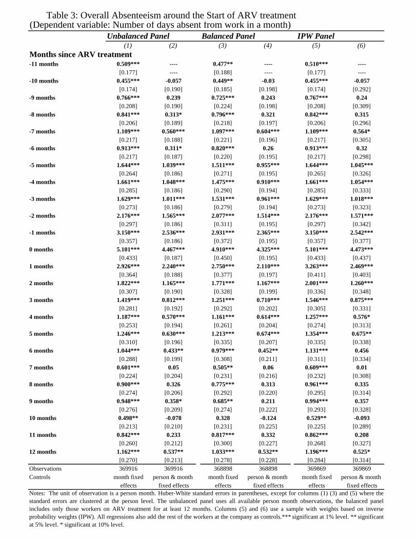
Table 3: Overall Absenteeism around the Start of ARV treatment(Dependent variable: Number of days absent from work in a month)
Unbalanced Panel Balanced Panel IPW Panel(1) (2) (3) (4) (5) (6)
Months since ARV treatment-11 months 0.509*** ---- 0.477** ---- 0.510*** ----
[0.177] ---- [0.188] ---- [0.177] -----10 months 0.455*** -0.057 0.449** -0.03 0.455*** -0.057
[0.174] [0.190] [0.185] [0.198] [0.174] [0.292]-9 months 0.766*** 0.239 0.725*** 0.243 0.767*** 0.24
[0.208] [0.190] [0.224] [0.198] [0.208] [0.309]-8 months 0.841*** 0.313* 0.796*** 0.321 0.842*** 0.315
[0.206] [0.189] [0.218] [0.197] [0.206] [0.296]-7 months 1.109*** 0.560*** 1.097*** 0.604*** 1.109*** 0.564*
[0.217] [0.188] [0.221] [0.196] [0.217] [0.305]-6 months 0.913*** 0.311* 0.820*** 0.26 0.913*** 0.32
[0.217] [0.187] [0.220] [0.195] [0.217] [0.298]-5 months 1.644*** 1.039*** 1.511*** 0.955*** 1.644*** 1.045***
[0.264] [0.186] [0.271] [0.195] [0.265] [0.326]-4 months 1.661*** 1.048*** 1.475*** 0.910*** 1.661*** 1.054***
[0.285] [0.186] [0.290] [0.194] [0.285] [0.333]-3 months 1.629*** 1.011*** 1.531*** 0.961*** 1.629*** 1.018***
[0.273] [0.186] [0.279] [0.194] [0.273] [0.323]-2 months 2.176*** 1.565*** 2.077*** 1.514*** 2.176*** 1.571***
[0.297] [0.186] [0.311] [0.195] [0.297] [0.342]-1 months 3.150*** 2.536*** 2.931*** 2.365*** 3.150*** 2.542***
[0.357] [0.186] [0.372] [0.195] [0.357] [0.377]0 months 5.101*** 4.467*** 4.910*** 4.325*** 5.101*** 4.473***
[0.433] [0.187] [0.450] [0.195] [0.433] [0.437]1 months 2.926*** 2.240*** 2.750*** 2.110*** 3.263*** 2.469***
[0.364] [0.188] [0.377] [0.197] [0.411] [0.403]2 months 1.822*** 1.165*** 1.771*** 1.167*** 2.001*** 1.260***
[0.307] [0.190] [0.328] [0.199] [0.336] [0.348]3 months 1.419*** 0.812*** 1.251*** 0.710*** 1.546*** 0.875***
[0.281] [0.192] [0.292] [0.202] [0.305] [0.331]4 months 1.187*** 0.570*** 1.161*** 0.614*** 1.257*** 0.576*
[0.253] [0.194] [0.261] [0.204] [0.274] [0.313]5 months 1.246*** 0.630*** 1.213*** 0.674*** 1.354*** 0.675**
[0.310] [0.196] [0.335] [0.207] [0.335] [0.338]6 months 1.044*** 0.433** 0.979*** 0.452** 1.131*** 0.456
[0.288] [0.199] [0.308] [0.211] [0.311] [0.334]7 months 0.601*** 0.05 0.505** 0.06 0.609*** 0.01
[0.224] [0.204] [0.231] [0.216] [0.232] [0.308]8 months 0.900*** 0.326 0.775*** 0.313 0.961*** 0.335
[0.274] [0.206] [0.292] [0.220] [0.295] [0.314]9 months 0.948*** 0.358* 0.685** 0.211 0.994*** 0.357
[0.276] [0.209] [0.274] [0.222] [0.293] [0.328]10 months 0.498** -0.078 0.328 -0.124 0.529** -0.093
[0.213] [0.210] [0.231] [0.225] [0.225] [0.289]11 months 0.842*** 0.233 0.817*** 0.332 0.862*** 0.208
[0.260] [0.212] [0.300] [0.227] [0.268] [0.327]12 months 1.162*** 0.537** 1.033*** 0.532** 1.196*** 0.525*
[0.270] [0.213] [0.278] [0.228] [0.284] [0.314]Observations 369916 369916 368898 368898 369869 369869Controls month fixed person & month month fixed person & month month fixed person & month
effects fixed effects effects fixed effects effects fixed effectsNotes: The unit of observation is a person month. Huber-White standard errors in parentheses, except for columns (1) (3) and (5) where thestandard errors are clustered at the person level. The unbalanced panel uses all available person month observations, the balanced panelincludes only those workers on ARV treatment for at least 12 months. Columns (5) and (6) use a sample with weights based on inverseprobability weights (IPW). All regressions also add the rest of the workers at the company as controls.*** significant at 1% level. ** significantat 5% level. * significant at 10% level.

Appendix Table 1: Descriptive Statistics
Mean SD N
Information for those receiving ARV treatment CD4 at treatment start 163 136 427 CD4 after 6 months 268 183 237 CD4 after 12 months 296 192 181 Age 42.65 8.28 441 Percent Male 0.82 0.39 441
Absenteeism Information (everyone)
Monthly sickdays 0.32 2.07 369916 Monthly ordinary leave 0.80 2.02 369916
Notes: SD is the standard deviation and N is the sample size. The information on absences are based on the sample included in Table 2.
Top Related