


Languages
Pages
Legal


History Matters i
By Arun S. Muralidhar Managing Director, FX Concepts, Inc
& Chairman, Mcube Investment Technologies LLC
Address: 80 Saratoga Drive, West Windsor, NJ 08550 Ph: 212-554-6831
Email: [email protected]

History Matters
Abstract
When deciding between two competing external managers or investment strategies, investors are faced with a troubling issue: how to compare these options if the two histories are not identical. There is a tendency to drop off
excess data to compare the two options, but this discards useful information for the investment option with a longer history. We demonstrate that new risk-adjusted performance measures make an important contribution to gleaning
relevant data from complete histories. In addition, we demonstrate why information ratios may be inadequate measures of skill as assumed by many
researchers, especially when time is taken into consideration.

“We had to add a third dimension: the time dimension…..If you don’t add time, you’ll find nothing.” Zhichun Jing, Chinese archaeologist, National Geographic,
July 2003 Introduction
Suppose a pension fund manager has to choose between two external managers –
one with a historical track record going back seven years and another with only a
five-year track record. If the two generate similar returns per unit of risk, then the
bias has been to hire the one with more experience. But life is never so easy and
typically, return and risk numbers, along with length of data histories, are wildly
different thereby adding confusion to the decision. For example, is the manager
with the longer history preferred to the one with a shorter history if the manager
with a longer history has a lower annualized excess return over the benchmark?
Generally, the selection favors the manager with the higher excess return
regardless of length of history. A similar problem is faced by investment
managers who must choose between competing investment strategies, where often
the availability of data (or lack thereof) determines the period over which rules
can be tested. To overcome this problem, investors often consider dropping
“excess data” to make an “apples to apples” comparison, but this decision to
disregard any available data is a flaw in the way these evaluations are conducted
as it penalizes the manager with longer histories or the strategy with longer data
availability.

Time and “Luck versus Skill”
One of the earliest papers to address the issue of time as it relates to skill is that of
Ambarish and Seigel (1996). They demonstrated that outperformance over a
benchmark unfortunately does not tell the investor whether the external manager
or mutual fund manager is skillful. It does not provide the investor with a measure
of confidence that they can have that the alpha is generated by skill-based
processes. Critical factors involved in answering the luck versus skill question
include time (or length of data history), desired degree of confidence, investment
returns of the portfolio and benchmark, standard deviation of the portfolio and the
benchmark, and the degree of correlation between the two. The problem is there
can be a lot of noise in performance data, and the more volatile the portfolio and
the excess return series of a manager, the greater the noise and, hence, greater the
time needed to resolve this question. They demonstrate that the minimum number
of data points or history H, should be large enough for skill to emerge from the
noise or, equivalently,
H>2
2)(
2)1(
21
21
2
221
)2(
−−
−
+−
BBrr
BBSσσ
σσρσσ (1)
where 1 is the manager, B is the benchmark, r denotes the return, σ denotes the
standard deviation, ρ is the correlation of returns between the manager and the
benchmark, and S is the number of standard deviations for a given confidence
level. One can see that their paper is a variant of, but a simpler version of

statistical process control alternatives such as Philips and Yashchin (1999). ii The
details for the derivation of equation (1) are provided in Appendix 1 for the
interested reader.
If the tracking error of portfolio 1 versus the benchmark is defined as the standard
deviation of excess returns, it is trivial to define TE(1) as follows:
TE(1) = )2( 21
21 BB σσρσσ +− (2)
Note that the second term in the numerator of the confidence in skill calcula tion
or equation (1) is the same as the square of the tracking error of portfolio 1 versus
the benchmark. Ambarish and Seigel (1996) suggest that even a 300 basis point
outperformance may require 175 years of data to claim with 84% confidence that
the manager is skillful, and hence skill may be in short supply or impossible to
detect given the length of histories within the industry. iii Muralidhar and U (1997)
and Muralidhar (1999) recognize that H is available as investors know the length
of performance history and solve for the degree of confidence, S instead. This
converts the analysis of required time to one of confidence in skill – a more
meaningful measure for investors.
Equation (1) makes it clear that the confidence in skill is intricately linked to the
information ratio (IR). The annualized information ratio is equal to the annualized
excess return divided by the annualized tracking error or, alternatively,

IR(1) = [r(1)-r(B)]/TE(1) (3)
The Sharpe ratio, often considered the parent to the information ratio is the return
of the active strategy minus the risk free rate, divided by the standard deviation of
the strategy. As a result and using (2) and (3), equation (1) can be rewritten in
terms of S, where S is a function of IR.
−−<
)1(2)1(
22
TEIRHS
Bi σσ (4)
The confidence in skill is derived from converting S to percentage terms for a
normal distribution or alternative the cumulative probability of a unit normal with
standard deviation of S. Define C(S1) as the cumulative probability of a unit
normal with standard deviation of S for fund 1, and this will be the measure of
confidence in skill. This measure will lie between 0% and 100% and hence acts as
a probability measure. For example, when S is equal to 1, then C(S) = 84%. Also,
when the second term in equation (4), or
−)1(2
22
TEBi σσ
is generally small or
insignificant, the IR and length of data history will largely determine the
confidence in skill. This is the case when tracking error is substantial and driven
largely by a low correlation between the portfolio and the benchmark (i.e., σi
≅σb). As a result, two portfolios with identical variances, information ratios and
tracking errors but differing only in length of history will have different
confidence in skill – longer the history, greater the confidence.
Why Information Ratios are Inadequate Statistics to Establish Skill
In this section we demonstrate first why the information ratio is an incomplete
statistic and further how time can cause an investor to select low information
ratios over high ones. Both analyses will be important in deriving a single risk-
adjusted performance measure that incorporates histories (or time) directly.
Muralidhar (2003) demonstrates that clients are making a big mistake when they
seek to maximize information ratios on active decisions. This paper extends a
conclusion first derived by Modigliani and Modigliani (1997) who argue that
information ratios tell the investor very little about the potential risk-adjusted
return that can be achieved and they show that even a negative information ratio
strategy can have a high (exceeding that of the benchmark) risk-adjusted return.
Yet, Grinold and Kahn (1999) make three distinct claims that appear to be
incorrect: (i) “Larger information ratios are better than smaller,” (page 6); (ii)
“The notion of success is captured and quantified by the information ratio,” (page
110); and (iii) “every investor seeks the strategy or manager with the highest
information ratio,” (page 125). In short, new measures of risk-adjusted
performance have been derived that adjust for tracking error correctly, but give
clients a lot of information about risk-adjusted return and portfolio construction.

These measures are known as the M2 and M3 measures respectively. The details
on these measures are provided in Appendix 2 and briefly summarized for the M3
below.
Two investment opportunities will typically have different variances and
correlations to the benchmark, in turn leading to different tracking errors relative
to the benchmark. This is a difficult comparison with too many moving parts. In
order to compare the two, it is recommended that the investor needs to invest in
the active strategy, the risk- less asset and benchmark to ensure: (a) the volatility
of this composite is equal to that of the benchmark (Modigliani and Modigliani
1997); and (b) the tracking error of this composite is equal to the target tracking
error (Muralidhar 2000). The second is achieved by ensuring that the newly
created composite portfolio has a correlation equal to a target correlation (derived
from the fact that there is a target tracking error and that the volatility of the
benchmark and that of the composite are equal). The M3 measure extends
Modigliani and Modigliani (1997) by recognizing that the investor has to consider
basis points of risk-adjusted performance after ensuring that correlations of
various funds versus the benchmark are also equal, thereby ensuring that the
tracking errors are equal.
Assume that the investor is willing to tolerate a certain target annualized tracking
error around the benchmark, say 300 bps (TE(target)).iv The investor essentially
wants to earn the highest risk-adjusted alpha for given tracking error and variance

of the portfolio. Now define a, b, and (1-a-b) as the proportions invested in the
active strategy, the benchmark, and the risk- less asset. Let CAP, be the correlation
adjusted portfolio and therefore the returns of a CAP,
r(CAP-1) = a*r(1) + (1-a-b)*r(F) + b*r(B) (5)
The solution for a, b and (1-a-b) is provided in Appendix 2 and Muralidhar
(2001) demonstrates that the M3 is the only measure (among alpha, Sharpe ratio,
information ratio and M2) that ranks investments identical to those based on
confidence in skill (or using equation (4)).
Equation (4) provides another valuable conclusion as it transparently
demonstrates that while the information ratio is an important element in
determining the confidence in skill, it is quite possible that the IR can provide
misleading results as the relationship between the two need not be linear
(Muralidhar 2001). One can easily see in equation (4) that it is possible to have a
higher confidence in the skill in a manager/strategy with a lower annualized
excess of a competing option if the length of history is long enough. As a result,
information ratios in isolation can give inaccurate indications of confidence in
skill or the attractiveness of risk-adjusted returns of an investment opportunity.
Alternative Measures of Performance that Incorporate Time
Knowing that a manager is highly skillful or a strategy has embedded skill is not
sufficient to convince the investor to adopt the same. For example, one may have
a high confidence in skill in a strategy (e.g., 90% confidence that excess returns
are skill-based), but if it only generates 0.1% of excess performance it is not going
to be adequate to help pay the pension benefits or keep an investment manager in
business. Hence one needs a measure of performance that incorporates time (or
confidence in skill) and a measure of returns that can be achieved. Muralidhar
(2002) demonstrates that the M3 is preferred to all other measures of risk-adjusted
performance as (i) it includes investments in all assets, including cash and the
passive benchmark, to produce the highest risk-adjusted return for a tracking error
target; and (ii) it is the only measure that ranks portfolios (measured over the
same time period) identical to rankings based on the confidence in skill measure
discussed above.
As a result, a new measure, called the SHARAD measure (Skill, History and
Risk-Adjusted measure) is created through the product of the confidence in skill
and the M3. This new measure exploits the fact that the “C(S)” measure is a
probability measure (extracted from equation (4)) that has dependence on the time
horizon of the data series and that the M3 measure provides appropriate risk
adjustment and guidance on portfolio construction and expresses risk-adjusted
performance in basis points. As a result, we can look at the SHARAD measure as
a probability-adjusted performance measure (or as an expected risk-adjusted
measure) by defining it for an active strategy 1 very simply, for a given tracking
error budget, as
SHARAD (1) = C(S1)*r(CAP-1) (6)
The “S” measure relates to the confidence that the CAP returns are skill-based (as
opposed to using raw returns), and C(S1) is the cumulative probability of a unit
normal with standard deviation of S. This revised measure now will have all the
attractive properties of the M3, but through the C(S) term accounts for time in a
manner that is consistent with the skill evaluation. v For managers with identical
data histories, this adjustment will have no impact in changing rankings, but for
different data histories one should see interesting results. In the next section, we
examine some data from mutual funds to see what the impact is of such
adjustments.
Effect of History on Ranking Active Strategies
We examine data for 10 US equity mutual funds (all ranked 5-star by
Morningstar) with different inception dates through August 1999. These funds
are ordered based on their annualized return since inception and shown in Table 1.
These funds are compared to the S&P500 index (benchmark) for the respective
start date of the fund. This data set was chosen to broadly represent funds that

have a high rating by the traditional rating agencies and to demonstrate the
importance of the time adjustment.
<INSERT TABLE 1 HERE>
The data ranges from as much as 20 years (Funds 4 and 10) to as little as 11.5
years (Fund 6). Normally, all additional data beyond 11.5 years would need to be
excluded to compare these funds. We have assumed a fixed risk free rate of 5%
for all funds to estimate the M2 (Sharpe ratios), and M3. In addition, we assume a
M3 target tracking error of an annualized 10% for all funds regardless of data
history. vi For completeness and for those not familiar with the M3 measure, the
recommended allocation to the mutual fund, benchmark and cash using this
method are also provided for each of the funds. The lower part of Table 1
provides the various returns, ratios and statistics using the measures described
above. Table 2 provides the ranks of each fund for the various parameters by
which a fund may be evaluated.
<INSERT TABLE 2 HERE>
To help the reader who is unfamiliar with these techniques understand the impact
of different time horizons, we provide the same tables in Appendix 3 using 10
years of data through August 1999 for all funds (i.e., identical data histories). The
key results about the superiority of the M3 methodology are demonstrated in these
Appendix tables as the risk-adjusted performance is expressed in performance
units, rankings are identical to those on confidence in skill, and information is
provided on portfolio construction. In this setup, the SHARAD rankings are
identical to the M3 rankings.
The following critical observations can be made from Tables 1 and 2, where the
inception dates for the different funds are as per their respective data histories:
• The rankings differ between the Sharpe or M2 and information
ratio, and further between the Sharpe and the M3. All three measures
show a healthy disregard for absolute performance or excess performance
over the benchmark as evidenced by the low correlation of ranks.
• A poor fund cannot be saved by a long data history alone as
demonstrated by Funds 4 and 10. The SHARAD of these funds ranks
poorly in this subset, even though they have the longest data history of the
funds. The converse is true for Fund 6, where the short history is not a
constraint on the confidence in skill.
• The M3 no longer provides ranks that are identical to those based
on skill when adjustments are made for length of history in the analysis
(Fund 4).
• All other measures, with the exception of confidence in risk-
adjusted performance, unfortunately, do not provide ranks that are
identical with the SHARAD. Even the confidence in risk-adjusted excess
is coincidentally identical to the SHARAD. For example, if the data
horizon for Fund 7 is changed to 20 years, then this is no longer the case
(even though the two measures are highly correlated). Hence, in
situations where there is a difference in performance history, other
measures will need to be replaced by the SHARAD.
• Inspite of the relative superiority of the M3 over the M2/Sharpe or
Information Ratio, rankings can be reversed when an adjustment is made
for time. Fund 4 has a lower ranking with SHARAD than with M3
excess, whereas Fund 7 improves its rank.
• The fund with the best SHARAD, Fund 3, does not have the
highest raw excess, or Sharpe, or even the longest data history. This
reflects the complex inter-relationships between return, volatility,
correlation and time.
• In this setup, the information ratio seems to have the greatest
correlation of ranks with other risk adjusted performance measures. One
can see why the IR correlates highly with the confidence in skill and as a
result with M3. This may explain its reasonably strong correlation with
the SHARAD measure. While this was not the case in the tables in the
Appendix where the data histories are identical, the relatively high
correlation of ranks may also explain why some analysts favor the
information ratio as highlighted in Gupta, Prajogi and Stubbs (1999) or in
Grinold and Kahn (1999).

Caveats and Extensions
In this setup we have evaluated individual funds, but investors normally invest in
multiple managers or strategies. This is a non- issue as the SHARAD measure can
also be used for multiple fund portfolios and hence lends itself to use by
institutional investors who normally hire more than one manager or by investment
managers who adopt more than one strategy. The key issue is whether the history
is an accurate predictor of the future and this is an open question as changes to the
investment process or personnel can affect future performance. Moreover, the
difficulty when using these evaluations for external managers or mutual funds is
whether the confidence in skill is vested in the organization or in individual
portfolio managers. The same analysis can be conducted on performance that is
attributed to models versus portfolio managers.
Conclusions
This paper sought to address a shortcoming of the existing range of risk-adjusted
performance measures, namely their inability to rank funds on an equivalent basis
if the funds had different lengths of performance histories. Ignoring the length of
history of an active manager or an active strategy can be dangerous as there is
useful information to be gleaned from this variable (on the confidence in skill).
We show that the SHARAD measure, which is in effect a probability adjusted
risk-adjusted performance measure has two elements to it: the first directly

incorporates time (and the skill evaluation), whereas the second provides risk-
adjusted basis points of performance (and information on optimal portfolio
construction). There will always be difficulties in distinguishing actual skill from
presumed skill, and further ensuring consistency in skill, but the periodic
application of this measure as more time is added to the history will demonstrate
whether ex-ante measures are good predictors of true skill. This paper
demonstrates that the final ranking among competing strategies is a complex
evaluation of return, variance, correlation with the benchmark and time and hence
simpler measures, while easy to calculate, may provide investors with incorrect
recommendations if they ignore the time dimension. History does matter!

Tables
Table 1 Fund Fund Fund Fund Fund Fund Fund Fund Fund Fund
1 2 3 4 5 6 7 8 9 10 Fund Return 25.16% 23.43% 22.46% 21.93% 21.39% 21.34% 20.97% 20.76% 19.22% 18.21% Fund Std. Dev. 25.55% 25.36% 15.61% 22.09% 15.98% 13.71% 18.98% 14.69% 19.90% 16.52% BM Return 19.18% 15.66% 18.76% 17.24% 19.91% 17.99% 18.26% 18.60% 17.53% 17.24% BM Std. Dev. 13.36% 14.87% 15.00% 14.99% 14.90% 13.06% 15.01% 13.11% 14.83% 14.99% Risk Free Rate 5.00% 5.00% 5.00% 5.00% 5.00% 5.00% 5.00% 5.00% 5.00% 5.00% Correlation 0.70 0.79 0.86 0.83 0.74 0.83 0.86 0.92 0.89 0.91 Target Correlation 0.72 0.77 0.78 0.78 0.77 0.71 0.78 0.71 0.77 0.78 Tracking Error 12.19% 10.48% 0.61% 7.10% 1.08% 0.65% 3.98% 1.58% 5.07% 1.53% a-Allocation to Fund 49% 63% 147% 88% 84% 151% 117% 294% 140% 201% b-Allocation to Benchmark 7% -8% -53% -30% 11% -60% -49% -233% -89% -123% c-Allocation to Risk-Free 44% 45% 7% 42% 6% 9% 32% 39% 49% 22% Time Horizon (Yrs) 11.75 11.92 15.25 20.00 15.58 11.50 14.33 11.67 15.75 20.00
Returns/Ratios Raw excess 5.98% 7.77% 3.70% 4.69% 1.48% 3.34% 2.72% 2.16% 1.69% 0.97% Sharpe 0.79 0.73 1.12 0.77 1.03 1.19 0.84 1.07 0.71 0.80 M 2 15.54% 15.81% 21.78% 16.49% 20.28% 20.56% 17.63% 19.06% 15.60% 16.99% Information Ratio 0.49 0.74 6.08 0.66 1.36 5.13 0.68 1.36 0.33 0.63 r(CAP) - 10% Tracking Error 15.84% 15.80% 23.23% 16.19% 20.30% 21.80% 17.20% 19.69% 13.72% 16.50% M 3 excess -3.34% 0.14% 4.47% -1.06% 0.39% 3.81% -1.06% 1.08% -3.81% -0.74% Confidence in Skill -Raw 48.68% 79.74% 100.00% 76.33% 99.97% 100.00% 75.58% 99.84% 25.44% 72.66% Confidence in Skill -M 3 12.63% 51.88% 95.97% 31.84% 56.06% 90.18% 34.42% 64.43% 6.53% 36.96% SHARAD 2.00% 8.20% 22.29% 5.16% 11.38% 19.66% 5.92% 12.68% 0.90% 6.10%
Table 2 Rank Raw Return 1 2 3 4 5 6 7 8 9 10 Raw excess 2 1 4 3 9 5 6 7 8 10 Sharpe 7 9 2 8 4 1 5 3 10 6 Information Ratio 9 5 1 7 4 2 6 3 10 8 r(CAP) - 10% Tracking Error 8 9 1 7 3 2 5 4 10 6 M 3 excess 9 5 1 7 4 2 8 3 10 6 Confidence in Skill -M 3 9 5 1 8 4 2 7 3 10 6 SHARAD 9 5 1 8 4 2 7 3 10 6 Time Horizon (Yrs) 8 7 5 1 4 10 6 9 3 1
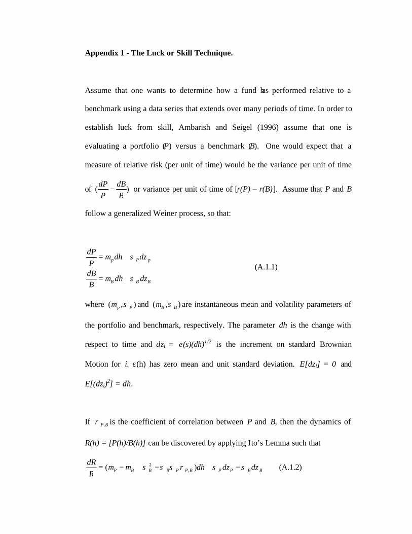
Appendix 1 - The Luck or Skill Technique.
Assume that one wants to determine how a fund has performed relative to a
benchmark using a data series that extends over many periods of time. In order to
establish luck from skill, Ambarish and Seigel (1996) assume that one is
evaluating a portfolio (P) versus a benchmark (B). One would expect that a
measure of relative risk (per unit of time) would be the variance per unit of time
of )(B
dBP
dP− or variance per unit of time of [r(P) – r(B)]. Assume that P and B
follow a generalized Weiner process, so that:
BBB
pPp
dzdhB
dB
dzdhP
dP
σµ
σµ
+=
+= (A.1.1)
where ),( Pp σµ and ),( BB σµ are instantaneous mean and volatility parameters of
the portfolio and benchmark, respectively. The parameter dh is the change with
respect to time and dzi = ε(s)(dh)1/2 is the increment on standard Brownian
Motion for i. ε(h) has zero mean and unit standard deviation. E[dzi] = 0 and
E[(dzi)2] = dh.
If BP,ρ is the coefficient of correlation between P and B, then the dynamics of
R(h) = [P(h)/B(h)] can be discovered by applying Ito’s Lemma such that
BBPPBPPBBBP dzdzdhR
dRσσρσσσµµ −+−+−= )( ,
2 (A.1.2)

Now define the stochastic variable dw such that
BBPPR dzdzdw σσσ −= (A.1.3)
where
BPBPPBR ,222 2 ρσσσσσ −+= (A.1.4)
which is the square of the tracking error (TE(P)) of portfolio P versus the
benchmark, B.
Then, as in any simple Brownian motion, R(s) can be defined in the following
way:
−−
−= hhRhR B
BP
PR 22exp].exp[)0()(
22 σµ
σµεσ
(A.1.5)
where ε is the standard normal variable, and exp[] stands for exponential. The
first exponential term in (A.1.5) is the noise (or luck) and the second exponential
term is the signal (or skill). Therefore, for skill embedded in managing portfolio
P to dominate noise associated with returns from luck, it must be the case that the
history of the fund (or number of data observations), S, satisfies the following
equation; namely that
H>2
2)(
2)(
2,
22
22
)2(
−−
−
+−
BP BP
BBPBPPS
σµ
σµ
σσσρσ (A.1.6)
Where S is the number of standard deviations for a given confidence level.


Appendix 2 - The M2 and M3 Measures of Risk-Adjusted Performance
The M2 Measure
Modigliani and Modigliani (1997) make an important contribution by showing
that the portfolio and the benchmark must have the same risk to compare them in
terms of basis points of risk-adjusted performance. They propose that the portfolio
be leveraged or deleveraged using the risk-free asset. If B is the benchmark being
compared to portfolio 1, the leverage factor, d, is defined as follows:
d = σB /σ1 (A.2.1)
Figure 1 demonstrates this transformation. It creates a new portfolio, called the
risk-adjusted portfolio (RAP), whose return r(RAP) is equal to the leverage factor
multiplied by the original return plus one minus the leverage factor multiplied by
the risk-free rate. Thus, if portfolio F is the risk- less asset with zero standard
deviation and is uncorrelated with other portfolios, the risk-adjusted return
r(RAP) = d*r(actual portfolio) +(1-d)r(F), (A.2.2)
where σRAP = σB (A.2.3)
The correlation of the original portfolio to the benchmark is identical to the
correlation of the RAP to the benchmark, as “leverage or deleverage” using the
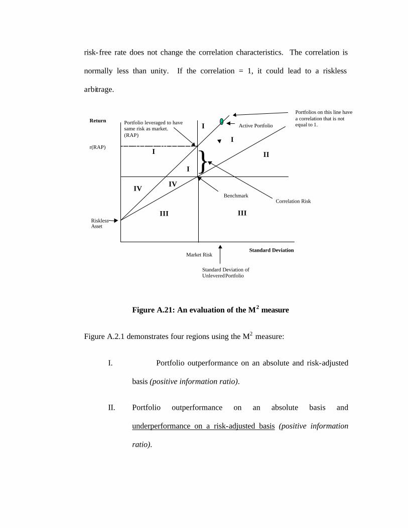
risk-free rate does not change the correlation characteristics. The correlation is
normally less than unity. If the correlation = 1, it could lead to a riskless
arbitrage.
Figure A.21: An evaluation of the M2 measure
Figure A.2.1 demonstrates four regions using the M2 measure:
I. Portfolio outperformance on an absolute and risk-adjusted
basis (positive information ratio).
II. Portfolio outperformance on an absolute basis and
underperformance on a risk-adjusted basis (positive information
ratio).
Standard Deviation
Return
IV
I II
IIIRisklessAsset
III
Market Risk
r(RAP)
Portfolio leveraged to havesame risk as market.(RAP)
I
Active Portfolio
Benchmark
I
IV
I
Portfolios on this line havea correlation that is notequal to 1.
}Correlation Risk
Standard Deviation ofUnlevered Portfolio

III. Portfolio underperformance on an absolute and risk-adjusted basis
(negative information ratio).
IV. Portfolio underperformance on an absolute basis and
outperformance on a risk-adjusted basis (negative information
ratio).
It shows that making this adjustment can reverse peer rankings of mutual funds or
managers. The rankings are shown to be identical using the Sharpe ratio measure
as the principle is similar. The M2 measure, however, was preferred as it
expressed risk-adjusted performance in terms of basis points of outperformance
and provides guidance on assets allocated to the external manager (allocation of
d) and the risk free asset (allocation of 1-d). The paper also discards the use of
the information ratio as it could lead to incorrect decisions as is evident from
Figure A.2.1.
The M2 adjustment made the comparison in terms of basis points of
outperformance by ensuring all portfolios had the same variance as the
benchmark. The one major shortcoming was that two funds, normalized for the
benchmark volatility, could have different correlations with the benchmarks and
hence different tracking errors. Tracking error is important to investors, especially
institutional investors, because it provides a measure of the variability of a
manager’s returns around the benchmark. Investors would prefer, all else being
equal, funds with lower tracking error (and hence greater predictability in
returns). Hence these rankings could provide investors with incorrect information
about the relative risk-adjusted performance of funds.vii
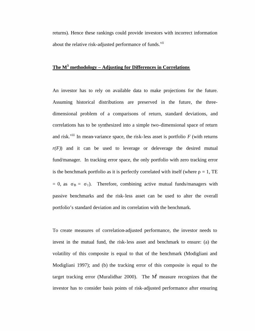
The M3 methodology – Adjusting for Differences in Correlations
An investor has to rely on available data to make projections for the future.
Assuming historical distributions are preserved in the future, the three-
dimensional problem of a comparisons of return, standard deviations, and
correlations has to be synthesized into a simple two-dimensional space of return
and risk.viii In mean-variance space, the risk- less asset is portfolio F (with returns
r(F)) and it can be used to leverage or deleverage the desired mutual
fund/manager. In tracking error space, the only portfolio with zero tracking error
is the benchmark portfolio as it is perfectly correlated with itself (where ρ = 1, TE
= 0, as σB = σ1). Therefore, combining active mutual funds/managers with
passive benchmarks and the risk- less asset can be used to alter the overall
portfolio’s standard deviation and its correlation with the benchmark.
To create measures of correlation-adjusted performance, the investor needs to
invest in the mutual fund, the risk- less asset and benchmark to ensure: (a) the
volatility of this composite is equal to that of the benchmark (Modigliani and
Modigliani 1997); and (b) the tracking error of this composite is equal to the
target tracking error (Muralidhar 2000). The M3 measure recognizes that the
investor has to consider basis points of risk-adjusted performance after ensuring

that correlations of various funds versus the benchmark are also equal, thereby
ensuring that the tracking errors are equal.
Assume that the investor is willing to tolerate a certain target annualized tracking
error around the benchmark, say 300 bps (TE(target)). The investor essentially
wants to earn the highest risk-adjusted alpha for given tracking error and variance
of the portfolio. Now define a, b, and (1-a-b) as the proportions invested in the
mutual fund, the benchmark, and the risk- less asset. Let CAP, be the correlation
adjusted portfolio and therefore the returns of a CAP,
r(CAP-1) = a*r(1) + (1-a-b)*r(F) + b*r(B) (A.2.5)
where the coefficients of each portfolio represent the optimal weight of that
specific portfolio to ensure complete risk adjustment. In addition, from the
constraint on tracking error, there is a unique target correlation between the CAP
and benchmark B (ρT,B) and is given by the equation for tracking error when σB =
σ1; namely,
ρT,B = 1 - 2
2
2)arg(
B
ettTEσ
(A.2.6)
By maximizing the r(CAP) subject to the condition that the variance be identical
to the benchmark, and its correlation to the benchmark equal to the target
correlation, we find that for mutual fund 1,

a = +)1(
)1(2,1
21
2,
2
B
BTB
ρσ
ρσ
−
− =
)1(
)1(2,1
2,
1 B
BTB
ρ
ρ
σσ
−
− (A.2.7)
b = BB
BT a ,11
, * ρσσ
ρ − (A.2.8)
If you substitute for “a” in equation (A.2.7), the allocation to the benchmark is
independent of variances and is only a function of the correlation terms. While b
and (1-a-b) may be greater than or less than zero (negative coefficients being
equivalent to shorting the futures contract relating to the benchmark and
borrowing at the risk-free rate), a is constrained to being positive as it is not
currently possible to short mutual funds, but a could be negative for an investment
strategy. ix
This method is preferred to the M2 as it: (a) expressed risk-adjusted performance
in basis points; (b) gives advice on portfolio construction – specifically between
the risk-free asset, the benchmark (passive investing) and the active portfolio
(active management); and (c) provides rankings that are identical with rankings
based on skill for equal time horizons. This measure also has the attractive
property of keeping a constant annualized tracking error target over all time
horizons.
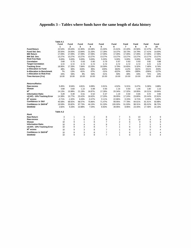
Appendix 3 – Tables where funds have the same length of data history
Table A.1Fund Fund Fund Fund Fund Fund Fund Fund Fund Fund
1 2 3 4 5 6 7 8 9 10Fund Return 22.54% 25.63% 21.90% 24.08% 21.00% 21.61% 22.40% 20.56% 22.47% 20.77%Fund Std. Dev. 25.50% 24.93% 13.84% 21.33% 17.28% 14.37% 18.73% 14.79% 17.41% 14.00%BM Return 17.09% 17.09% 17.09% 17.09% 17.09% 17.09% 17.09% 17.09% 17.09% 17.09%BM Std. Dev. 13.27% 13.27% 13.27% 13.27% 13.27% 13.27% 13.27% 13.27% 13.27% 13.27%Risk Free Rate 5.00% 5.00% 5.00% 5.00% 5.00% 5.00% 5.00% 5.00% 5.00% 5.00%Correlation 0.69 0.75 0.83 0.80 0.79 0.97 0.83 0.93 0.92 0.88Target Correlation 0.72 0.72 0.72 0.72 0.72 0.72 0.72 0.72 0.72 0.72Tracking Error 18.95% 17.33% 7.84% 13.33% 10.59% 3.79% 10.65% 5.32% 7.48% 6.74%a-Allocation to Fund 48% 60% 153% 85% 100% 663% 112% 342% 231% 203%b-Allocation to Benchmark 7% -13% -61% -37% -31% -622% -60% -285% -206% -117%c-Allocation to Risk-Free 44% 53% 8% 53% 31% 59% 48% 43% 75% 14%Time Horizon (Yrs) 10.00 10.00 10.00 10.00 10.00 10.00 10.00 10.00 10.00 10.00
Returns/RatiosRaw excess 5.45% 8.54% 4.81% 6.99% 3.91% 4.52% 5.31% 3.47% 5.38% 3.68%Sharpe 0.69 0.83 1.22 0.89 0.93 1.16 0.93 1.05 1.00 1.13M2 14.13% 15.98% 21.19% 16.87% 17.28% 20.34% 17.32% 18.95% 18.31% 19.94%Information Ratio 0.29 0.49 0.61 0.52 0.37 1.19 0.50 0.65 0.72 0.55r(CAP) - 10% Tracking Error 14.38% 15.77% 23.42% 16.62% 17.20% 39.95% 17.24% 23.80% 20.44% 22.91%M3 excess -2.71% -1.32% 6.33% -0.47% 0.11% 22.86% 0.15% 6.71% 3.35% 5.82%Confidence in Skill 45.58% 68.92% 96.57% 75.86% 71.47% 99.95% 77.78% 94.61% 91.91% 93.98%Confidence in Skill-M3 19.59% 33.82% 97.73% 44.15% 51.33% 100.00% 51.93% 98.31% 85.52% 96.72%SHARAD 2.82% 5.33% 22.88% 7.34% 8.83% 39.95% 8.95% 23.40% 17.48% 22.16%
Table A.2RankRaw Return 3 1 6 2 8 7 5 10 4 9Raw excess 3 1 6 2 8 7 5 10 4 9Sharpe 10 9 1 8 7 2 6 4 5 3Information Ratio 10 8 4 6 9 1 7 3 2 5r(CAP) - 10% Tracking Error 10 9 3 8 7 1 6 2 5 4M3 excess 10 9 3 8 7 1 6 2 5 4Confidence in Skill-M3 10 9 3 8 7 1 6 2 5 4SHARAD 10 9 3 8 7 1 6 2 5 4

Bibliography
Ambarish, R. and L. Seigel (1996). Time is the Essence. Risk. August 1996, 9(8).
Dowd, K (2000). Adjusting for Risk: An Improved Sharpe Ratio. International Review of
Economics and Finance. 9, 2000, pp.209-222.
Graham, J.R. and C.R. Harvey (1997). Grading the Performance of Market Timing
Newsletters. Financial Analysts Journal, 53(6):54-66.
Grinold, R.C., and Kahn, R.N. (1999). Active Portfolio Management: a Quantitative
Approach for Providing Superior Returns and Controlling Risk: Second Edition,
McGraw Hill.
Gupta, F., R. Prajogi, and E. Stubbs (1999). The Information Ratio and Performance. The
Journal of Portfolio Management, Fall, 26(1).
Hammond, D. (1997). Establishing Performance-Related Termination Thresholds for
Investment Management in Pension Fund Investment Management, ed. F. Fabozzi, Frank
Fabozzi Associates, New Hope, Pa.
Litterman, R., J. Longerstaey, J. Rosengarten, and K. Winkelmann (2001). The Green
Zone... assessing the Quality of Returns, The Journal of Performance Measurement,
Spring, 5(3).
McRae, D. (1999). Sharpe Ratio Alternatives. Managed Account Research. November
1999.
Modigliani, F. and L. Modigliani (1997). Risk-Adjusted Performance. The Journal of
Portfolio Management, 23(2):45-54.

Muralidhar, A (2000). Risk-Adjusted Performance – The Correlation Correction.
Financial Analysts Journal, 56(5):63-71.
Muralidhar, A (2001). Optimal Risk-Adjusted Portfolios with Multiple Managers,
Journal of Portfolio Management, Volume 27, Number 3, Spring 2001.
Muralidhar, A (2001). Innovations in Pension Fund Management, Stanford University
Press, Stanford, Ca.
Muralidhar, A. (2002). Skill, Horizon and Risk-Adjusted Performance, Journal of
Performance Measurement, Fall.
Muralidhar, A. (2003). Why Maximizing Information Ratios is Incorrect, working paper
submitted to the Financial Analysts Journal.
Philips, T. and E. Yashchin (1999). Monitoring Manager Performance Using Statistical
Process Controls. Forthcoming in Journal of Portfolio Management - 2003.
Sharpe, W. (1994). The Sharpe Ratio. Journal of Portfolio Management, 20(1): 49-59.
i My debt of gratitude to Prof. Franco Modigliani and Lester Seigel is immeasurable for the hours spent on discussing this topic. Thanks also to Sanjay Muralidhar and Kenneth Miranda. All errors are mine. ii One of the problems of Philips and Yashchin (1999) is that the user is required to specify an information ratio above which funds would be rated good. In the technique employed here, no such classification is required. iii This result is from outperformance engendered through 13.2% basis points of tracking error, where the benchmark standard deviation = 15%, the actual standard deviation = 25% and the correlation between the two was 0.9. iv This measure is independent of the level of tracking error and hence is applicable across all tracking error targets. v We obviously take a few liberties here with the use of S by assuming that S is an equality rather than an inequality. In addition, the rankings need not be exactly identical with the skill rankings as demonstrated later. vi This translates into different target correlations for each fund because of the differences in benchmark standard deviation over their respective histories. If two funds had an identical time horizon, the target correlation would be the same for both. vii In addition, when benchmark returns are negative (e.g., in currency mandates), the M2 measure will incorrectly rank underperforming funds with high volatility are preferred to funds with low volatility. This is a quirk of the method as it is generally assumed that benchmarks have positive returns. viii These are heroic assumptions to say the least. Some forecast needs to be made on expected outperformance, variability of performance to achieve this outperformance and correlations between portfolio and benchmark returns. Historical performance is one way of making forecasts, but the M-3

measure is independent of the forecasting technique. In addition, one must believe that markets are inefficient to conduct such analyses. ix This may change with the development of exchange-traded funds (ETFs) on active portfolios. In some cases it may be difficult to short the benchmark as well and then b will need to constrained to being greater than or equal to zero. This would not change the analysis of the measure. In general though, most benchmarks can be shorted either through their futures contract or through a swap.
Top Related