Internal Report

For Project

COME 10: 3D Visualization of Joints from MRI Data

Biomechanics of Hip Joint Capsule

March 30th, 2002

Prepared by: Anderson Maciel

Supervision: Dr. Ronan Boulic

Direction: Prof. Daniel Thalmann

Computer Graphics Lab (LIG) Institute of Computing and Multimedia Systems (ISIM)

School of Computer and Communication Sciences (I&C) Swiss Federal Institute of Technology (EPFL)

The National Center of Competence in Research Computer Aided and Image Guided Medical Interventions

(CO-ME)

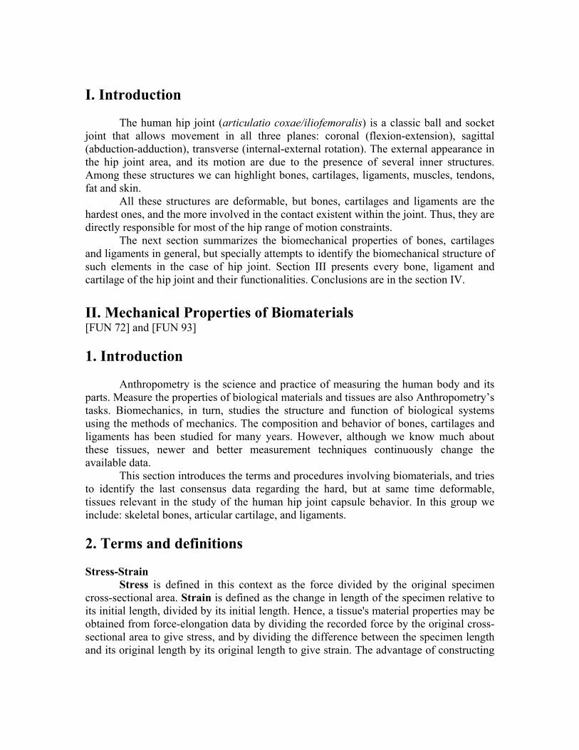
I. Introduction

The human hip joint (articulatio coxae/iliofemoralis) is a classic ball and socket joint that allows movement in all three planes: coronal (flexion-extension), sagittal (abduction-adduction), transverse (internal-external rotation). The external appearance in the hip joint area, and its motion are due to the presence of several inner structures. Among these structures we can highlight bones, cartilages, ligaments, muscles, tendons, fat and skin.

All these structures are deformable, but bones, cartilages and ligaments are the hardest ones, and the more involved in the contact existent within the joint. Thus, they are directly responsible for most of the hip range of motion constraints.

The next section summarizes the biomechanical properties of bones, cartilages and ligaments in general, but specially attempts to identify the biomechanical structure of such elements in the case of hip joint. Section III presents every bone, ligament and cartilage of the hip joint and their functionalities. Conclusions are in the section IV. II. Mechanical Properties of Biomaterials [FUN 72] and [FUN 93] 1. Introduction

Anthropometry is the science and practice of measuring the human body and its

parts. Measure the properties of biological materials and tissues are also Anthropometry’s tasks. Biomechanics, in turn, studies the structure and function of biological systems using the methods of mechanics. The composition and behavior of bones, cartilages and ligaments has been studied for many years. However, although we know much about these tissues, newer and better measurement techniques continuously change the available data.

This section introduces the terms and procedures involving biomaterials, and tries to identify the last consensus data regarding the hard, but at same time deformable, tissues relevant in the study of the human hip joint capsule behavior. In this group we include: skeletal bones, articular cartilage, and ligaments. 2. Terms and definitions Stress-Strain

Stress is defined in this context as the force divided by the original specimen cross-sectional area. Strain is defined as the change in length of the specimen relative to its initial length, divided by its initial length. Hence, a tissue's material properties may be obtained from force-elongation data by dividing the recorded force by the original cross-sectional area to give stress, and by dividing the difference between the specimen length and its original length by its original length to give strain. The advantage of constructing

a stress-strain diagram is that to a first approximation the stress-strain behavior is independent of the tissue dimensions.

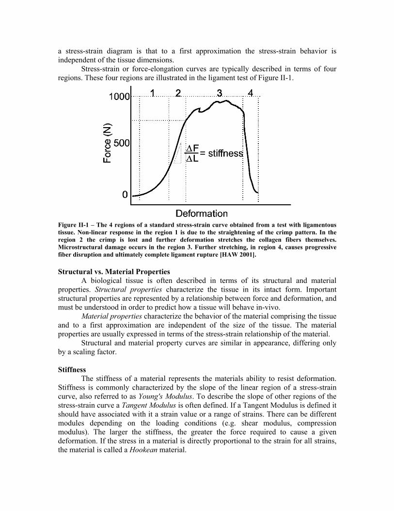
Stress-strain or force-elongation curves are typically described in terms of four regions. These four regions are illustrated in the ligament test of Figure II-1.

Figure II-1 – The 4 regions of a standard stress-strain curve obtained from a test with ligamentous tissue. Non-linear response in the region 1 is due to the straightening of the crimp pattern. In the region 2 the crimp is lost and further deformation stretches the collagen fibers themselves. Microstructural damage occurs in the region 3. Further stretching, in region 4, causes progressive fiber disruption and ultimately complete ligament rupture [HAW 2001]. Structural vs. Material Properties

A biological tissue is often described in terms of its structural and material properties. Structural properties characterize the tissue in its intact form. Important structural properties are represented by a relationship between force and deformation, and must be understood in order to predict how a tissue will behave in-vivo.

Material properties characterize the behavior of the material comprising the tissue and to a first approximation are independent of the size of the tissue. The material properties are usually expressed in terms of the stress-strain relationship of the material.

Structural and material property curves are similar in appearance, differing only by a scaling factor. Stiffness

The stiffness of a material represents the materials ability to resist deformation. Stiffness is commonly characterized by the slope of the linear region of a stress-strain curve, also referred to as Young's Modulus. To describe the slope of other regions of the stress-strain curve a Tangent Modulus is often defined. If a Tangent Modulus is defined it should have associated with it a strain value or a range of strains. There can be different modules depending on the loading conditions (e.g. shear modulus, compression modulus). The larger the stiffness, the greater the force required to cause a given deformation. If the stress in a material is directly proportional to the strain for all strains, the material is called a Hookean material.

Anisotropy and Non-homogeneity Ideal materials are isotropic and homogeneous. A material is called isotropic

when its properties are the same in each of three coordinate axes (x,y,z). Tensile and compressive properties may be different, but each respective property must be the same in three directions. A material is said to be homogeneous if it is made of the same material throughout. Biological tissues are anisotropic and non-homogeneous. Viscoelastic Properties

Biological tissues are viscoelastic materials. It means that their behavior is time and history dependent. A viscoelastic material possesses characteristics of stress-relaxation, creep, strain rate sensitivity, and hysteresis. Force-relaxation (or stress-relaxation) is a phenomenon that occurs in a tissue stretched and held at a fixed length. Over time the force present within the tissue continually declines. Force-relaxation is strain rate sensitive. In general, the higher the strain rate, the larger the peak force and subsequently the greater the magnitude of the force-relaxation. In contrast to stress-relaxation that occurs when a tissue’s length is held fixed, creep occurs when a constant force is applied across the tissue. If subjected to a constant tensile force, then a tissue elongates with time. The general shape of the displacement-time curve depends on the past loading history (e.g. peak force, loading rate).

Another time-dependent property is strain rate sensitivity. Different tissues show different sensitivities to strain rate. For example, there may be little difference in the stress-strain behavior of ligaments subjected to tensile tests varying in strain rate over three decades while bone properties may change considerably (this concept is discussed in more detail later in this report).

Besides, the loading and unloading curves obtained from a force-deformation test of biological tissues do not follow the same path. The difference in the calculated area under the loading and unloading curves is termed the area of hysteresis and represents the energy lost due to internal friction in the material. The amount of energy liberated or absorbed during a tensile test is defined as the integral of the force and the displacement. Hence the maximum energy absorbed at failure equals the area under the force-displacement curve.

Fung [FUN 93] in his QLV (Quasilinear Viscoelastic) theory suggested that if a step increase in elongation is imposed on the specimen, the stress developed will be a function of time (t) as well as of the material stretch ratio (λ). The history of the stress response, called the relaxation function (K(λ,t)), is assumed to be of the form (K(λ,t) = G(t)*T(λ)) in which G(t) is a normalized function of time, called the reduced relaxation function and T(λ) is a function of the stretch ratio alone, called the elastic response. Fung also proposed a function for defining the elastic response of the material under tension conditions [FUN 93]. Viscosity

The viscosity of a fluid is a measure of the fluid's resistance to flow. Viscosity of water is used as reference to calculate other fluids viscosity, and is considered to be 1. The capsule of diarthrodial joints is normally filled with a fluid of viscosity 10 called synovial fluid. This fluid helps to reduce friction and wear of articulating surfaces. Just for comparison, the viscosity of olive oil, for example, is 84 [HAW 2001].

Coefficient of Friction

The coefficient of friction is that fraction of the force transmitted across two bearing surfaces that must be used to initiate movement (µs -static friction) or keep the surfaces moving (µd -dynamic friction). The static coefficient of friction between two surfaces is always greater than the dynamic coefficient of friction. Joints of the human body are well designed to reduce the coefficient of friction between articulating surfaces. See the section 4 that is dedicated to cartilage. Testing procedures

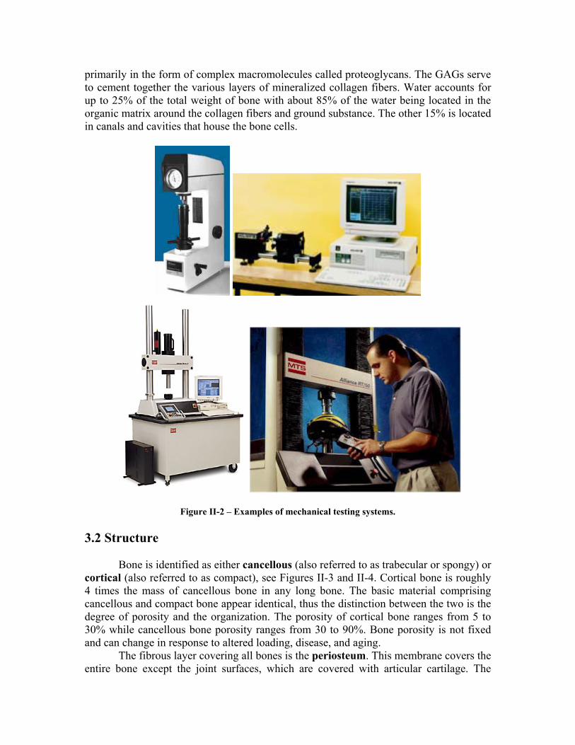
Structural properties of biological tissues are usually determined through some form of mechanical testing (e.g. tensile tests, compressive tests, bending and torsion tests). Customized workstations utilizing force transducers, clamps, and an actuator to control the distance between clamps are commonplace. Commercial systems are also available and vary in design depending on the type of tissue being studied (e.g. macroscopic vs. microscopic, hard tissue vs. soft tissue etc.) and the type of loading rates required. Instron [INS 2001] and MTS [MTS 2001] are the two most common suppliers of mechanical testing systems. Most systems allow either force control or length control. See pictures in Figure II-2.

Mechanical testing of tissue in-vivo is very difficult and hence not commonly performed. Some of the techniques that have been utilized include: 1) buckle transducers to monitor tendon and ligament forces, 2) telemetried pressure sensors to measure joint contact pressure, and 3) strain gauges to quantify bone and ligament strain. Some non-invasive approaches have also been employed. Ultrasound techniques have been used to detect changes in the speed of sound in different tissues and these changes have been correlated with the tissue's elastic properties.

Various imaging techniques have also been used to quantify tissue geometry and deformation [HAW 2001]. 3. Bones 3.1 Composition

Bone is a composite material consisting of both fluid and solid phases. Two main solid phases, one organic and another inorganic, give bones their hard structure. An organic extracellular collagenous matrix is impregnated with inorganic materials, especially hydroxyapatite Ca10(PO4)6(OH)2 (consisting of the minerals calcium and phosphate). Unlike collagen, apatite crystals are very stiff and strong. However, bones strength is higher than of either apatite or collagen, because similarly of what happens with concrete, the softer component prevents the stiff one from brittle cracking, while the stiff component prevents the soft one from yielding. The organic material gives bone its flexibility while the inorganic material gives bone its resilience.

Calcium and phosphate account for roughly 65 to 70% of the bone's dry weight. Collagen fibers compose approximately 95% of the extracellular matrix and account for 25 to 30% of the dry weight of bone. Surrounding the mineralized collagen fibers is a ground substance consisting of protein, polysaccharides, or glycosaminoglycans (GAGs),

primarily in the form of complex macromolecules called proteoglycans. The GAGs serve to cement together the various layers of mineralized collagen fibers. Water accounts for up to 25% of the total weight of bone with about 85% of the water being located in the organic matrix around the collagen fibers and ground substance. The other 15% is located in canals and cavities that house the bone cells.

Figure II-2 – Examples of mechanical testing systems.

3.2 Structure

Bone is identified as either cancellous (also referred to as trabecular or spongy) or cortical (also referred to as compact), see Figures II-3 and II-4. Cortical bone is roughly 4 times the mass of cancellous bone in any long bone. The basic material comprising cancellous and compact bone appear identical, thus the distinction between the two is the degree of porosity and the organization. The porosity of cortical bone ranges from 5 to 30% while cancellous bone porosity ranges from 30 to 90%. Bone porosity is not fixed and can change in response to altered loading, disease, and aging.

The fibrous layer covering all bones is the periosteum. This membrane covers the entire bone except the joint surfaces, which are covered with articular cartilage. The

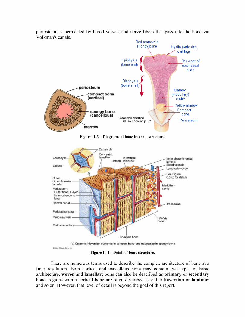
periosteum is permeated by blood vessels and nerve fibers that pass into the bone via Volkman's canals.

Figure II-3 – Diagrams of bone internal structure.

Figure II-4 – Detail of bone structure.

There are numerous terms used to describe the complex architecture of bone at a

finer resolution. Both cortical and cancellous bone may contain two types of basic architecture, woven and lamellar; bone can also be described as primary or secondary bone; regions within cortical bone are often described as either haversian or laminar; and so on. However, that level of detail is beyond the goal of this report.

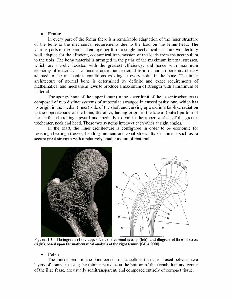
• Femur In every part of the femur there is a remarkable adaptation of the inner structure

of the bone to the mechanical requirements due to the load on the femur-head. The various parts of the femur taken together form a single mechanical structure wonderfully well-adapted for the efficient, economical transmission of the loads from the acetabulum to the tibia. The bony material is arranged in the paths of the maximum internal stresses, which are thereby resisted with the greatest efficiency, and hence with maximum economy of material. The inner structure and external form of human bone are closely adapted to the mechanical conditions existing at every point in the bone. The inner architecture of normal bone is determined by definite and exact requirements of mathematical and mechanical laws to produce a maximum of strength with a minimum of material.

The spongy bone of the upper femur (to the lower limit of the lesser trochanter) is composed of two distinct systems of trabeculae arranged in curved paths: one, which has its origin in the medial (inner) side of the shaft and curving upward in a fan-like radiation to the opposite side of the bone; the other, having origin in the lateral (outer) portion of the shaft and arching upward and medially to end in the upper surface of the greater trochanter, neck and head. These two systems intersect each other at right angles.

In the shaft, the inner architecture is configured in order to be economic for resisting shearing stresses, bending moment and axial stress. Its structure is such as to secure great strength with a relatively small amount of material.

Figure II-5 – Photograph of the upper femur in coronal section (left), and diagram of lines of stress (right), based upon the mathematical analysis of the right femur. [GRA 2000]

• Pelvis

The thicker parts of the bone consist of cancellous tissue, enclosed between two layers of compact tissue; the thinner parts, as at the bottom of the acetabulum and center of the iliac fosse, are usually semitransparent, and composed entirely of compact tissue.

3.3 Material Properties and Related Behavior

Cancellous bone is actually extremely anisotropic and inhomogeneous. Cortical bone, on the other hand, is approximately linear elastic, transversely isotropic and relatively homogenous. The material properties of bone are generally determined using mechanical testing procedures, however ultrasonic techniques have also been employed. Force-deformation (structural properties) or stress-strain (material properties) curves can be determined by means of such tests. However, the properties of bone and most biological tissues depend on the freshness of the tissue. These properties can change within a matter of minutes if allowed to dry out. Cortical bone, for example, has an ultimate strain of around 1.2% when wet and about 0.4% if the water content is not maintained. Thus, it is very important to keep bone specimens wet during testing.

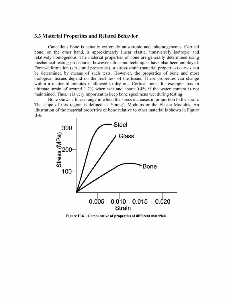
Bone shows a linear range in which the stress increases in proportion to the strain. The slope of this region is defined as Young's Modulus or the Elastic Modulus. An illustration of the material properties of bone relative to other material is shown in Figure II-6.

Figure II-6 – Comparative of properties of different materials.

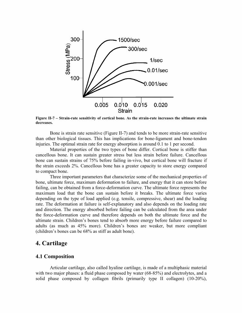
Figure II-7 – Strain-rate sensitivity of cortical bone. As the strain-rate increases the ultimate strain decreases.

Bone is strain rate sensitive (Figure II-7) and tends to be more strain-rate sensitive

than other biological tissues. This has implications for bone-ligament and bone-tendon injuries. The optimal strain rate for energy absorption is around 0.1 to 1 per second.

Material properties of the two types of bone differ. Cortical bone is stiffer than cancellous bone. It can sustain greater stress but less strain before failure. Cancellous bone can sustain strains of 75% before failing in-vivo, but cortical bone will fracture if the strain exceeds 2%. Cancellous bone has a greater capacity to store energy compared to compact bone.

Three important parameters that characterize some of the mechanical properties of bone, ultimate force, maximum deformation to failure, and energy that it can store before failing, can be obtained from a force-deformation curve. The ultimate force represents the maximum load that the bone can sustain before it breaks. The ultimate force varies depending on the type of load applied (e.g. tensile, compressive, shear) and the loading rate. The deformation at failure is self-explanatory and also depends on the loading rate and direction. The energy absorbed before failing can be calculated from the area under the force-deformation curve and therefore depends on both the ultimate force and the ultimate strain. Children’s bones tend to absorb more energy before failure compared to adults (as much as 45% more). Children’s bones are weaker, but more compliant (children’s bones can be 68% as stiff as adult bone). 4. Cartilage 4.1 Composition Articular cartilage, also called hyaline cartilage, is made of a multiphasic material with two major phases: a fluid phase composed by water (68-85%) and electrolytes, and a solid phase composed by collagen fibrils (primarily type II collagen) (10-20%),

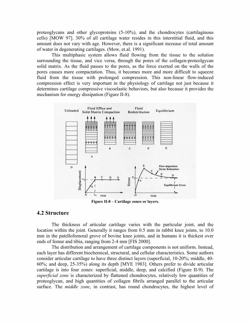
proteoglycans and other glycoproteins (5-10%), and the chondrocytes (cartilaginous cells) [MOW 97]. 30% of all cartilage water resides in this interstitial fluid, and this amount does not vary with age. However, there is a significant increase of total amount of water in degenerating cartilages. (Mow, et.al. 1991). This multiphasic system allows fluid flowing from the tissue to the solution surrounding the tissue, and vice versa, through the pores of the collagen-proteolgycan solid matrix. As the fluid passes to the pores, as the force exerted on the walls of the pores causes more compactation. Thus, it becomes more and more difficult to squeeze fluid from the tissue with prolonged compression. This non-linear flow-induced compression effect is very important in the physiology of cartilage not just because it determines cartilage compressive viscoelastic behaviors, but also because it provides the mechanism for energy dissipation (Figure II-8).

Figure II-8 – Cartilage zones or layers.

4.2 Structure

The thickness of articular cartilage varies with the particular joint, and the location within the joint. Generally it ranges from 0.5 mm in rabbit knee joints, to 10.0 mm in the patellofemoral grove of bovine knee joints, and in humans it is thickest over ends of femur and tibia, ranging from 2-4 mm [FIS 2000].

The distribution and arrangement of cartilage components is not uniform. Instead, each layer has different biochemical, structural, and cellular characteristics. Some authors consider articular cartilage to have three distinct layers (superficial, 10-20%; middle, 40-60%; and deep, 25-35%) along its depth [MYE 1983]. Others prefer to divide articular cartilage is into four zones: superficial, middle, deep, and calcified (Figure II-9). The superficial zone is characterized by flattened chondrocytes, relatively low quantities of proteoglycan, and high quantities of collagen fibrils arranged parallel to the articular surface. The middle zone, in contrast, has round chondrocytes, the highest level of

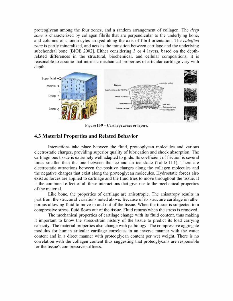
proteoglycan among the four zones, and a random arrangement of collagen. The deep zone is characterized by collagen fibrils that are perpendicular to the underlying bone, and columns of chondrocytes arrayed along the axis of fibril orientation. The calcified zone is partly mineralized, and acts as the transition between cartilage and the underlying subchondral bone [BIOE 2002]. Either considering 3 or 4 layers, based on the depth-related differences in the structural, biochemical, and cellular compositions, it is reasonable to assume that intrinsic mechanical properties of articular cartilage vary with depth.

Superficial

Middle

Deep

Bone

Figure II-9 – Cartilage zones or layers.

4.3 Material Properties and Related Behavior

Interactions take place between the fluid, proteoglycan molecules and various electrostatic charges, providing superior quality of lubrication and shock absorption. The cartilaginous tissue is extremely well adapted to glide. Its coefficient of friction is several times smaller than the one between the ice and an ice skate (Table II-1). There are electrostatic attractions between the positive charges along the collagen molecules and the negative charges that exist along the proteoglycan molecules. Hydrostatic forces also exist as forces are applied to cartilage and the fluid tries to move throughout the tissue. It is the combined effect of all these interactions that give rise to the mechanical properties of the material.

Like bone, the properties of cartilage are anisotropic. The anisotropy results in part from the structural variations noted above. Because of its structure cartilage is rather porous allowing fluid to move in and out of the tissue. When the tissue is subjected to a compressive stress, fluid flows out of the tissue. Fluid returns when the stress is removed.

The mechanical properties of cartilage change with its fluid content, thus making it important to know the stress-strain history of the tissue to predict its load carrying capacity. The material properties also change with pathology. The compressive aggregate modulus for human articular cartilage correlates in an inverse manner with the water content and in a direct manner with proteoglycan content per wet weight. There is no correlation with the collagen content thus suggesting that proteoglycans are responsible for the tissue's compressive stiffness.

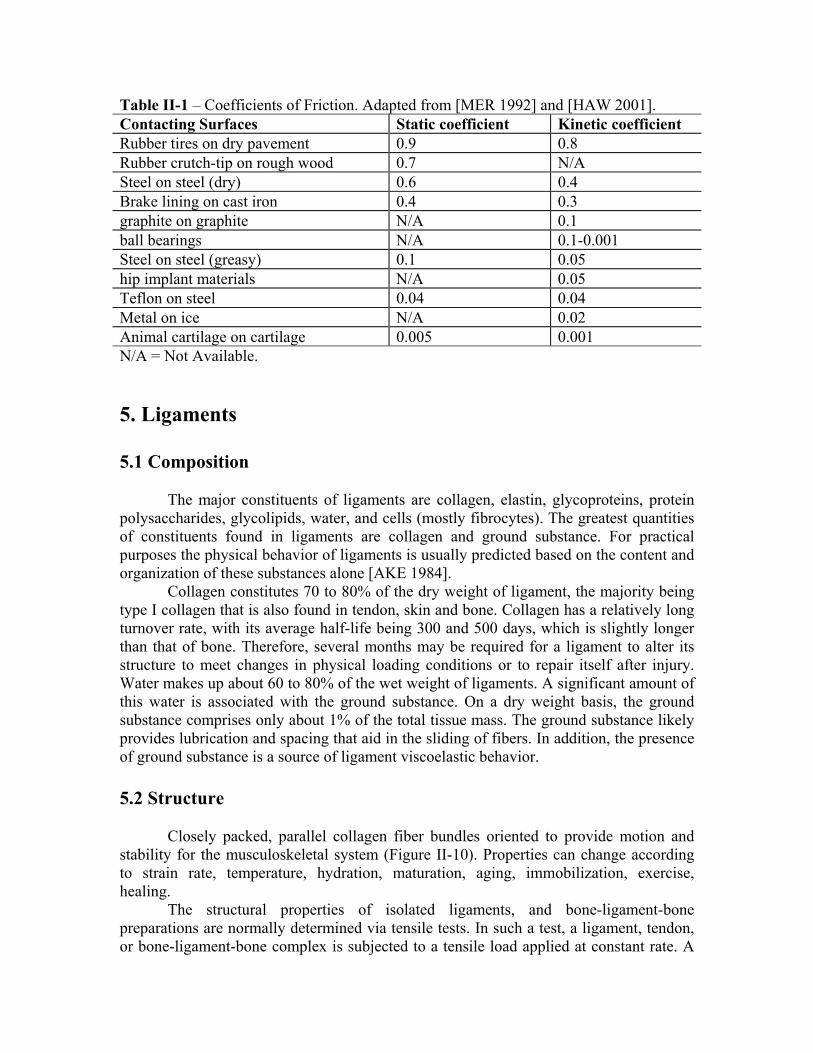
Table II-1 – Coefficients of Friction. Adapted from [MER 1992] and [HAW 2001]. Contacting Surfaces Static coefficient Kinetic coefficient Rubber tires on dry pavement 0.9 0.8 Rubber crutch-tip on rough wood 0.7 N/A Steel on steel (dry) 0.6 0.4 Brake lining on cast iron 0.4 0.3 graphite on graphite N/A 0.1 ball bearings N/A 0.1-0.001 Steel on steel (greasy) 0.1 0.05 hip implant materials N/A 0.05 Teflon on steel 0.04 0.04 Metal on ice N/A 0.02 Animal cartilage on cartilage 0.005 0.001 N/A = Not Available.

5. Ligaments 5.1 Composition

The major constituents of ligaments are collagen, elastin, glycoproteins, protein

polysaccharides, glycolipids, water, and cells (mostly fibrocytes). The greatest quantities of constituents found in ligaments are collagen and ground substance. For practical purposes the physical behavior of ligaments is usually predicted based on the content and organization of these substances alone [AKE 1984].

Collagen constitutes 70 to 80% of the dry weight of ligament, the majority being type I collagen that is also found in tendon, skin and bone. Collagen has a relatively long turnover rate, with its average half-life being 300 and 500 days, which is slightly longer than that of bone. Therefore, several months may be required for a ligament to alter its structure to meet changes in physical loading conditions or to repair itself after injury. Water makes up about 60 to 80% of the wet weight of ligaments. A significant amount of this water is associated with the ground substance. On a dry weight basis, the ground substance comprises only about 1% of the total tissue mass. The ground substance likely provides lubrication and spacing that aid in the sliding of fibers. In addition, the presence of ground substance is a source of ligament viscoelastic behavior. 5.2 Structure

Closely packed, parallel collagen fiber bundles oriented to provide motion and stability for the musculoskeletal system (Figure II-10). Properties can change according to strain rate, temperature, hydration, maturation, aging, immobilization, exercise, healing.

The structural properties of isolated ligaments, and bone-ligament-bone preparations are normally determined via tensile tests. In such a test, a ligament, tendon, or bone-ligament-bone complex is subjected to a tensile load applied at constant rate. A

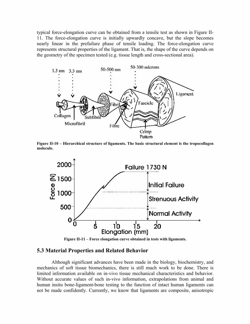
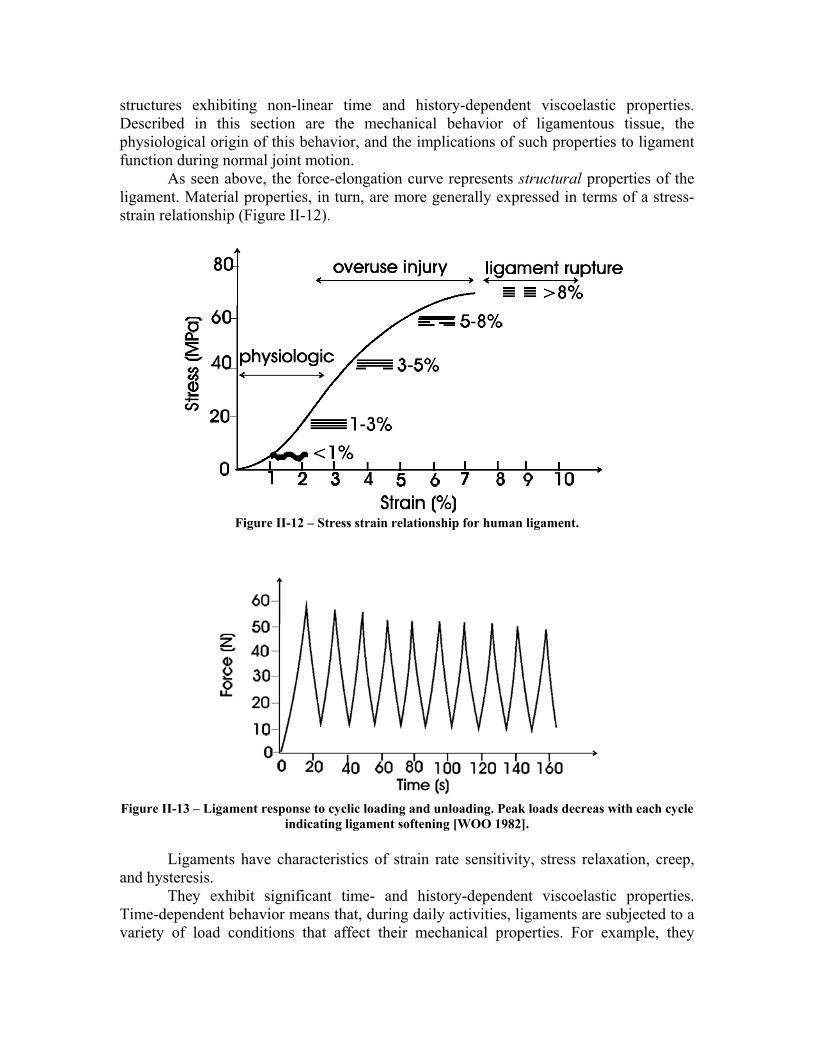
typical force-elongation curve can be obtained from a tensile test as shown in Figure II-11. The force-elongation curve is initially upwardly concave, but the slope becomes nearly linear in the prefailure phase of tensile loading. The force-elongation curve represents structural properties of the ligament. That is, the shape of the curve depends on the geometry of the specimen tested (e.g. tissue length and cross-sectional area).

Figure II-10 – Hierarchical structure of ligaments. The basic structural element is the tropocollagen molecule.

Figure II-11 – Force elongation curve obtained in tests with ligaments.

5.3 Material Properties and Related Behavior

Although significant advances have been made in the biology, biochemistry, and mechanics of soft tissue biomechanics, there is still much work to be done. There is limited information available on in-vivo tissue mechanical characteristics and behavior. Without accurate values of such in-vivo information, extrapolations from animal and human insitu bone-ligament-bone testing to the function of intact human ligaments can not be made confidently. Currently, we know that ligaments are composite, anisotropic

structures exhibiting non-linear time and history-dependent viscoelastic properties. Described in this section are the mechanical behavior of ligamentous tissue, the physiological origin of this behavior, and the implications of such properties to ligament function during normal joint motion.

As seen above, the force-elongation curve represents structural properties of the ligament. Material properties, in turn, are more generally expressed in terms of a stress-strain relationship (Figure II-12).

Figure II-12 – Stress strain relationship for human ligament.

Figure II-13 – Ligament response to cyclic loading and unloading. Peak loads decreas with each cycle

indicating ligament softening [WOO 1982].

Ligaments have characteristics of strain rate sensitivity, stress relaxation, creep, and hysteresis.

They exhibit significant time- and history-dependent viscoelastic properties. Time-dependent behavior means that, during daily activities, ligaments are subjected to a variety of load conditions that affect their mechanical properties. For example, they

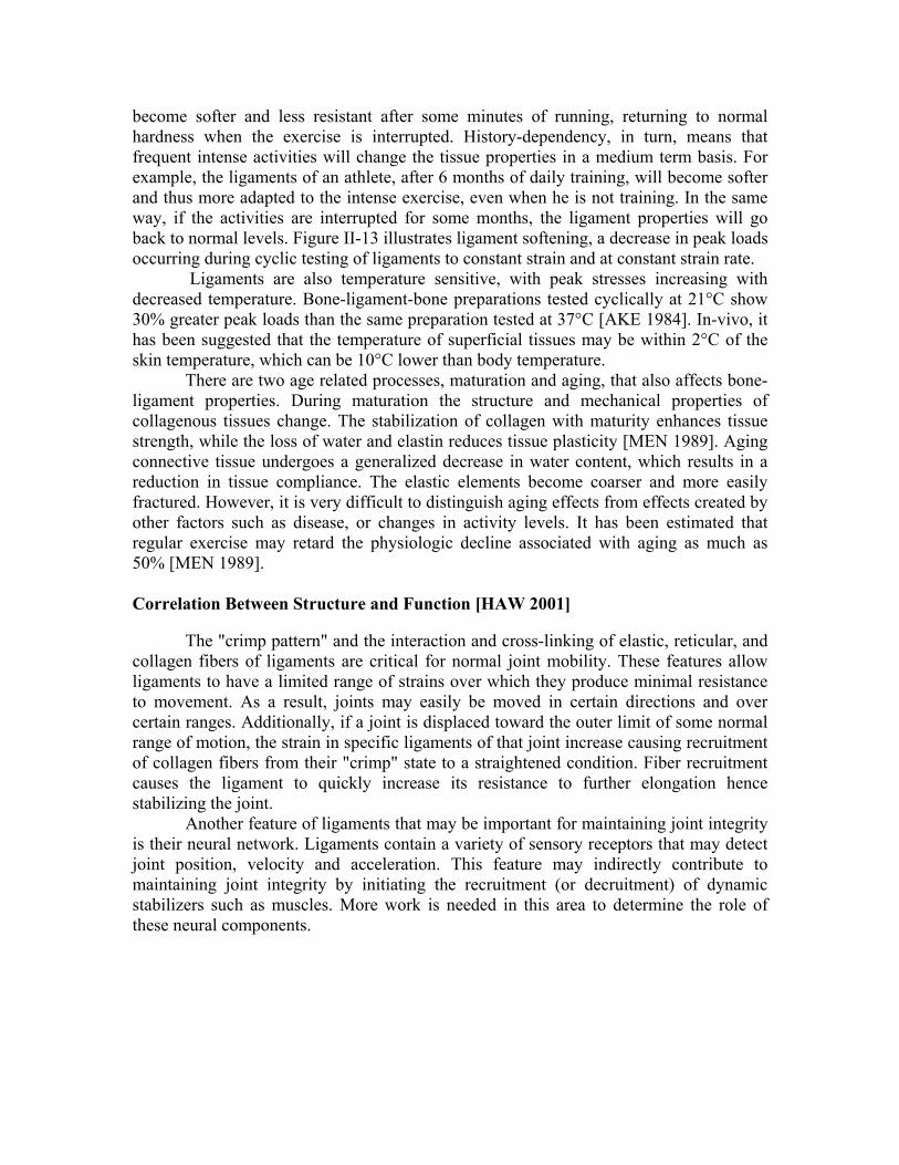
become softer and less resistant after some minutes of running, returning to normal hardness when the exercise is interrupted. History-dependency, in turn, means that frequent intense activities will change the tissue properties in a medium term basis. For example, the ligaments of an athlete, after 6 months of daily training, will become softer and thus more adapted to the intense exercise, even when he is not training. In the same way, if the activities are interrupted for some months, the ligament properties will go back to normal levels. Figure II-13 illustrates ligament softening, a decrease in peak loads occurring during cyclic testing of ligaments to constant strain and at constant strain rate.

Ligaments are also temperature sensitive, with peak stresses increasing with decreased temperature. Bone-ligament-bone preparations tested cyclically at 21°C show 30% greater peak loads than the same preparation tested at 37°C [AKE 1984]. In-vivo, it has been suggested that the temperature of superficial tissues may be within 2°C of the skin temperature, which can be 10°C lower than body temperature.

There are two age related processes, maturation and aging, that also affects bone-ligament properties. During maturation the structure and mechanical properties of collagenous tissues change. The stabilization of collagen with maturity enhances tissue strength, while the loss of water and elastin reduces tissue plasticity [MEN 1989]. Aging connective tissue undergoes a generalized decrease in water content, which results in a reduction in tissue compliance. The elastic elements become coarser and more easily fractured. However, it is very difficult to distinguish aging effects from effects created by other factors such as disease, or changes in activity levels. It has been estimated that regular exercise may retard the physiologic decline associated with aging as much as 50% [MEN 1989]. Correlation Between Structure and Function [HAW 2001]

The "crimp pattern" and the interaction and cross-linking of elastic, reticular, and collagen fibers of ligaments are critical for normal joint mobility. These features allow ligaments to have a limited range of strains over which they produce minimal resistance to movement. As a result, joints may easily be moved in certain directions and over certain ranges. Additionally, if a joint is displaced toward the outer limit of some normal range of motion, the strain in specific ligaments of that joint increase causing recruitment of collagen fibers from their "crimp" state to a straightened condition. Fiber recruitment causes the ligament to quickly increase its resistance to further elongation hence stabilizing the joint.

Another feature of ligaments that may be important for maintaining joint integrity is their neural network. Ligaments contain a variety of sensory receptors that may detect joint position, velocity and acceleration. This feature may indirectly contribute to maintaining joint integrity by initiating the recruitment (or decruitment) of dynamic stabilizers such as muscles. More work is needed in this area to determine the role of these neural components.

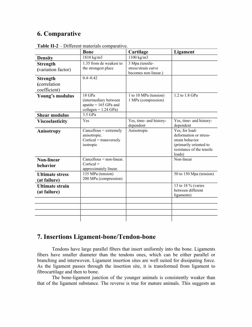
6. Comparative Table II-2 – Different materials comparative. Bone Cartilage Ligament Density 1810 kg/m3 1100 kg/m3

Strength (variation factor)

1.35 from de weakest to the strongest place

3 Mpa (tensile-stress/strain curve becomes non-linear.)

Strength (correlation coefficient)

0.4~0.42

Young’s modulus 18 GPa (intermediary between apatite = 165 GPa and collagen = 1.24 GPa)

1 to 10 MPa (tension) 1 MPa (compression)

1.2 to 1.8 GPa

Shear modulus 3.5 GPa

Viscoelasticity Yes Yes, time- and history-dependent

Yes, time- and history-dependent

Anisotropy Cancellous = extremely anisotropic. Cortical = transversely isotropic

Anisotropic Yes, for load-deformation or stress-strain behavior (primarily oriented to resistance of the tensile loads)

Non-linear behavior

Cancellous = non-linear. Cortical = approximately linear.

Non-linear

Ultimate stress (at failure)

135 MPa (tension) 200 MPa (compression)

50 to 150 Mpa (tension)

Ultimate strain (at failure)

13 to 18 % (varies between different ligaments)

7. Insertions Ligament-bone/Tendon-bone

Tendons have large parallel fibers that insert uniformly into the bone. Ligaments fibers have smaller diameter than the tendons ones, which can be either parallel or branching and interwoven. Ligament insertion sites are well suited for dissipating force. As the ligament passes through the insertion site, it is transformed from ligament to fibrocartilage and then to bone.

The bone-ligament junction of the younger animals is consistently weaker than that of the ligament substance. The reverse is true for mature animals. This suggests an

asynchronous rate of maturation between the bone-ligament junction and that of the ligament substance.

Two different types of insertions exist: direct, more common, the tendon or ligament crosses the mineralization front and progresses from fibril to fibrocartilage (usually less than 0.6 mm), to mineralized fibrocartilage (less than 0.4 mm), and finally to bone; indirect, less common, it inserts into bone through the periosteum, with short fibers that are anchored to the bone.

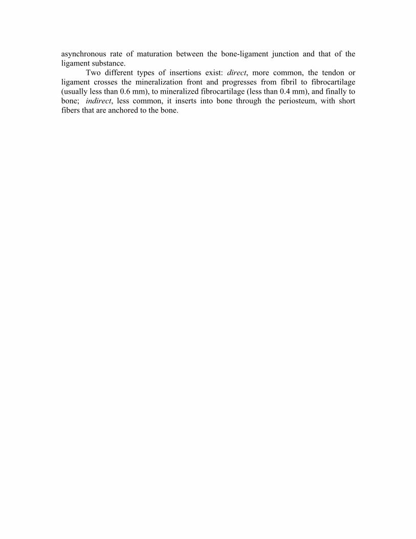
III. Hip Joint Elements

Right-hip front-view Right-hip posterior-view Left-hip medial-view

Figure III-1 – Views of the Hip Joint [GRA 2000]

1. Bones:

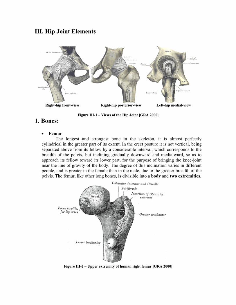
• Femur The longest and strongest bone in the skeleton, it is almost perfectly

cylindrical in the greater part of its extent. In the erect posture it is not vertical, being separated above from its fellow by a considerable interval, which corresponds to the breadth of the pelvis, but inclining gradually downward and medialward, so as to approach its fellow toward its lower part, for the purpose of bringing the knee-joint near the line of gravity of the body. The degree of this inclination varies in different people, and is greater in the female than in the male, due to the greater breadth of the pelvis. The femur, like other long bones, is divisible into a body and two extremities.

Figure III-2 – Upper extremity of human right femur [GRA 2000]

The upper extremity, the more important in this work, presents for examination a head, a neck, a greater and a lesser trochanter. The head, which is globular and forms rather more than a hemisphere, is directed upward, medialward, and a little forward, the greater part of its convexity being above and in front. Its surface is smooth, coated with cartilage in the fresh state, except over an ovoid depression, the fovea capitis femoris, which is situated a little below and behind the center of the head, and gives attachment to the ligamentum teres.

The femur is ossified from five centers: one for the body, one for the head, one for each trochanter, and one for the lower extremity. Of all the long bones, except the clavicle, it is the first to show traces of ossification; this commences in the middle of the body, at about the seventh week of fetal life, and rapidly extends upward and downward. The centers in the epiphyses appear in the following order: in the lower end of the bone, at the ninth month of fetal life (from this center the condyles and epicondyles are formed); in the head, at the end of the first year after birth; in the greater trochanter, during the fourth year; and in the lesser trochanter, between the thirteenth and fourteenth years. The order in which the epiphyses are joined to the body is the reverse of that of their appearance; they are not united until after puberty, the lesser trochanter being first joined, then the greater, then the head, and, finally, the inferior extremity, which is not united until the twentieth year.

• Pelvis (acetabulum)

Also called hip-bone, pelvis is a large, flattened, irregularly shaped bone, constricted in the center and expanded above and below. It meets its fellow on the opposite side in the middle line in front, and together they form the sides and anterior wall of the pelvic cavity. It consists of three parts, the ilium, ischium, and pubis, which are distinct from each other in the young subject, but are fused in the adult; the union of the three parts takes place in and around a large cup-shaped articular cavity, the acetabulum, which is situated near the middle of the outer surface of the bone. The ilium, so-called because it supports the flank, is the superior broad and expanded portion that extends upward from the acetabulum. The ischium is the lowest and strongest portion of the bone; it proceeds downward from the acetabulum, expands into a large tuberosity, and then, curving forward, forms, with the pubis, a large aperture, the obturator foramen. The pubis extends medialward and downward from the acetabulum and articulates in the middle line with the bone of the opposite side: it forms the front of the pelvis and supports the external organs of reproduction.

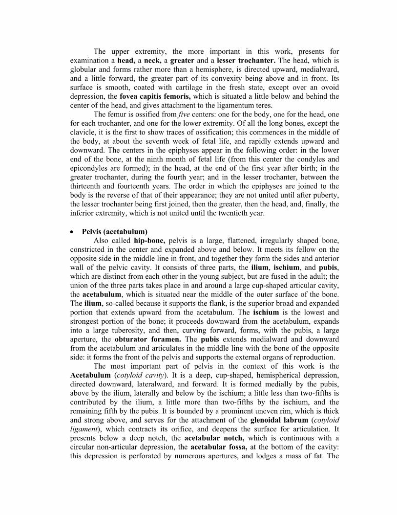
The most important part of pelvis in the context of this work is the Acetabulum (cotyloid cavity). It is a deep, cup-shaped, hemispherical depression, directed downward, lateralward, and forward. It is formed medially by the pubis, above by the ilium, laterally and below by the ischium; a little less than two-fifths is contributed by the ilium, a little more than two-fifths by the ischium, and the remaining fifth by the pubis. It is bounded by a prominent uneven rim, which is thick and strong above, and serves for the attachment of the glenoidal labrum (cotyloid ligament), which contracts its orifice, and deepens the surface for articulation. It presents below a deep notch, the acetabular notch, which is continuous with a circular non-articular depression, the acetabular fossa, at the bottom of the cavity: this depression is perforated by numerous apertures, and lodges a mass of fat. The

notch is converted into a foramen by the transverse ligament; through the foramen nutrient vessels and nerves enter the joint; the margins of the notch serve for the attachment of the ligamentum teres. The rest of the acetabulum is formed by a curved cartilaginous surface, the lunate surface, for articulation with the head of the femur.

Figure III-3 – Two acetabular views of the pelvis. At left, showing ligaments and muscles attachments; at right, the young pelvis in formation (the three parts of bone are not completely fused) [GRA 2000].

Summary

Head of the femur

Size: 2/3 of a sphere Fovea capitis

It is a depression on the head of the femur where the ligament teres (ligament of the head of the femur) is attached.

Location: below and behind the center of the articular surface of the head. Neck of the femur

Connects the head and shaft of the femur. Direction: anteriorly. Biomechanical effect: since both head of the femur and acetabulum face

anteriorly, a large part of the head of the femur is not covered by the acetabulum during normal standing.

Clinical application: only a small part of the articular surface of the head is tolerating weight. This area is located on the posterosuperior aspect of the head.

Acetabulum formed by three bones :

- ilium : superiorly - pubis : anteroinferiorly - ischium : posteroinferiorly

size: a little bit larger than half a sphere Acetabular labrum

fibrocartilage rim around the acetabulum. Labrum deepens the acetabulum. Acetabular notch

Inferior part of the acetabulum is incomplete and forms the acetabular notch.

2. Ligaments: The articular capsule and ligaments work as static stabilizers of the hip joint, especially the iliofemoral ligament, which tightens in extension enabling the hip to assume a stable close packed position; in the other hand, muscles are considered as dynamic stabilizers. Contrarily of what happens in other joints, the role of ligaments on determining the hip joint motion and range of motion is less significant. The articular capsule and the other 6 ligaments of hip joint are described bellow. However, it is known that these 7 structures are not separated. Actually, they are blended together to compose the complex of the articular capsule. The differences in names and classification are due to functional variations in thickness and orientation of fibers, as we can observe in the figure III-1.

• The Articular Capsule It is strong and dense. Above, it is attached to the margin of the acetabulum 5

to 6 mm beyond the glenoidal labrum behind; but in front, it is attached to the outer margin of the labrum, and, opposite to the notch where the margin of the cavity is deficient, it is connected to the transverse ligament, and by a few fibers to the edge of the obturator foramen (muscle). It surrounds the neck of the femur, and is attached, in front, to the intertrochanteric line; above, to the base of the neck; behind, to the neck, about 1.25 cm above the intertrochanteric crest; below, to the lower part of the neck, close to the lesser trochanter. From its femoral attachment some of the fibers are reflected upward along the neck as longitudinal bands, termed retinacula. The capsule is much thicker at the upper and forepart of the joint, where the greatest amount of resistance is required; behind and below, it is thin and loose. It consists of two sets of fibers, circular and longitudinal. The circular fibers, zona orbicularis, are most abundant at the lower and back part of the capsule, and form a sling or collar around the neck of the femur. Anteriorly, they blend with the deep surface of the iliofemoral ligament, and gain an attachment to the anterior inferior iliac spine. The longitudinal fibers are greatest in amount at the upper and front part of the capsule, where they are reinforced by distinct bands or accessory ligaments, of which the most important is the iliofemoral ligament.

• The Pubocapsular (also pubofemoral or ligamentum pubofemorale)

Attached, above, to the obturator crest and the superior ramus of the pubis; below, it blends with the capsule and with the deep surface of the vertical band of the iliofemoral ligament.

• The Iliofemoral

A band of great strength that lies in front of the joint; it is intimately connected with the capsule, and serves to strengthen it in this situation. It is attached, above, to the lower part of the anterior inferior iliac spine; below, it divides into two bands, one of which passes downward and is fixed to the lower part of the intertrochanteric line; the other is directed downward and lateralward and is attached to the upper part of the same line. Between the two bands there is a thinner part of the capsule. In some cases there is no division, and the ligament spreads out into a flat triangular band, which is attached to the whole length of the intertrochanteric line. This ligament is frequently called the Y-shaped ligament of Bigelow; and its upper band is sometimes named the iliotrochanteric ligament.

• The Teres Femoris (also ligamentum capitis femoris)

A triangular, somewhat flattened band implanted by its apex into the antero-superior part of the fovea capitis femoris; its base is attached by two bands, one into either side of the acetabular notch, and between these bony attachments it blends with the transverse ligament. It is ensheathed by the synovial membrane, and varies greatly in strength in different subjects; occasionally only the synovial fold exists, and in rare cases even this is absent. The ligament is made tense when the thigh is semiflexed and the limb then adducted or rotated outward; it is, on the other hand, relaxed when the limb is abducted. It has, however, little influence as a ligament.

• The Ischiocapsular (also ischiofemoral or ligamentum ischiofemorale)

Consists of a triangular band of strong fibers, which spring from the ischium below and behind the acetabulum, and blend with the circular fibers of the capsule.

• The Glenoidal Labrum (also acetabular lip or labrum acetabulare)

A fibrocartilaginous rim attached to the margin of the acetabulum, the cavity it deepens. At the same time it protects the edge of the bone, and fills up the inequalities of its surface. It bridges over the notch as the transverse ligament, and thus forms a complete circle, which closely surrounds the head of the femur and assists in holding it in its place. It is triangular on section, its base being attached to the margin of the acetabulum, while its opposite edge is free and sharp. Its two surfaces are invested by synovial membrane, the external one being in contact with the capsule, the internal one being inclined inward so as to narrow the acetabulum, and embrace the cartilaginous surface of the head of the femur. It is much thicker above and behind than below and in front, and consists of compact fibers.

• The Transverse Acetabular (also transversum acetabuli) It is in reality a portion of the glenoidal labrum, though differing from it in

having no cartilage cells among its fibers. It consists of strong, flattened fibers, which cross the acetabular notch, and convert it into a foramen through which the nutrient vessels enter in the joint.

Summary

Capsular ligament Capsule is thick, reinforced by strong ligaments. Capsular fibers run in the same direction as the neck of the femur. Capsule runs from acetabular labrum to intertrochantric line anteriorly. Capsule begins from acetabular labrum posteriorly also but it finishes short

of intertrochantric crest. Much of the neck of the femur is intracapsular The orbicular zone, usually considered as a part of the capsule, is a circular

ligament reinforcing the articular capsule around the neck of the femur. Pubofemoral ligament: Checks medial rotation and tightens on abduction Reinforces the capsule Attachments

- Proximal: superior branch of the pubis bone near the acetabulum - Distal: intertrochanteric line of the femur bone.

Iliofemoral ligament

It is one of the strongest ligaments in the body. Attachments

- proximal: antero-inferior portion of the ilium bone, also superior and posterosuperior rim of acetabulum. - distal: intertrochantric line. It has two divisions: lateral division attaches to greater trochanter; medial division attaches to lesser trochanter.

Direction: anterior to hip joint runs downwardly. Fibers are twisted. Function:

- Checks medial rotation and extension of the femur. - Prevents closed-packed position of the hip joint. - Checking adduction somewhat

Clinical application: One can stand with minimum muscular activity. During standing pelvis rolls backward and the lig. is tightened Ligament Teres Ligament of the head of the femur Shape: cylindrical Transmit blood vessels Attachments:

- Proximal: the pit of the head of the femur

- Distal: the acetabular notch. Ischiofemoral ligament

Attachments - proximal: ischium posterior and posteroinferior to the acetabular rim in the superior and lateral directions. - distal: posterosuperior aspect of the neck of the femur(where the neck meet the greater trochanter)

Function: checks medial rotation and extension of the femur. Glenoidal labrum The fibrocartilaginous edge which forms a ring around the circular outer border of

the acetabulum. Deepens the acetabulum.

Transverse acetabular ligament Spans the acetabular notch inferiorly Forms a bridge over the artery in the ligament of the femoral head.

3. Cartilages: The femoral head is covered by articular cartilage that is thick centrally and thin peripherally, conversely the acetabular cartilage is thicker peripherally. The opposing surfaces are regularly and reciprocally curved, and at any given time only 2/5th of the femoral head occupies the acetabulum. The labrum serves to convert the bony acetabulum into a true hemisphere as well as deepening it thus increasing joint stability. See Figure III-4. Summary

Acetabulum cartilage (Lunate surface): Horse-shoe-shaped area within the acetabulum covered by hyaline cartilage. There is an area in the center of the acetabulum not covered by hyaline cartilage,

the acetabular fosse. The head of the femur ligament moves within the acetabular fosse upon hip joint movements. Head of the femur:

The entire head is covered by articular cartilage except the fovea capitis where the ligamentum capitis attaches.

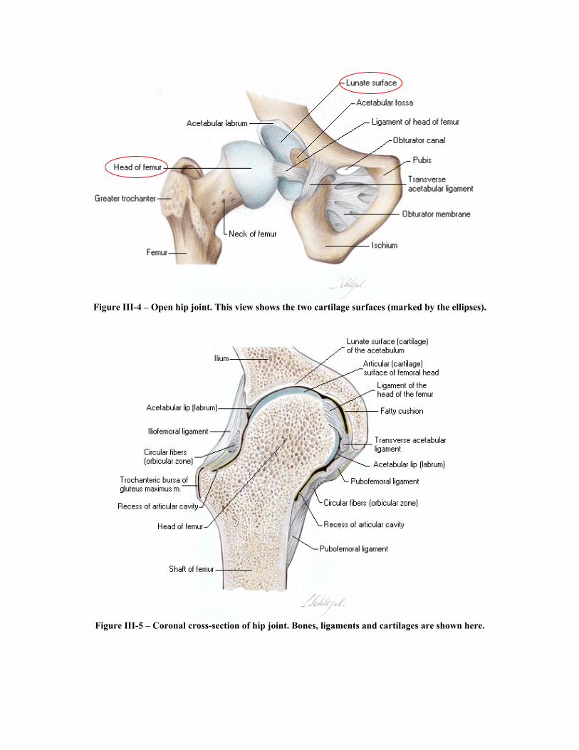
Figure III-4 – Open hip joint. This view shows the two cartilage surfaces (marked by the ellipses).

Figure III-5 – Coronal cross-section of hip joint. Bones, ligaments and cartilages are shown here.

4. Range of Motion

Range of motion of a joint is the set of possible positions for the joint. Basically, the constraints that define a range of motion are the presence, structure and composition of bones, cartilages, ligaments, muscles, fatty tissues and skin.

Two types of range of motion can be considered: - Active: measured while the person moves his/her members by himself/herself,

activating his/her muscles to move. - Passive: measured while the person is resting and a second one uses his/her hands

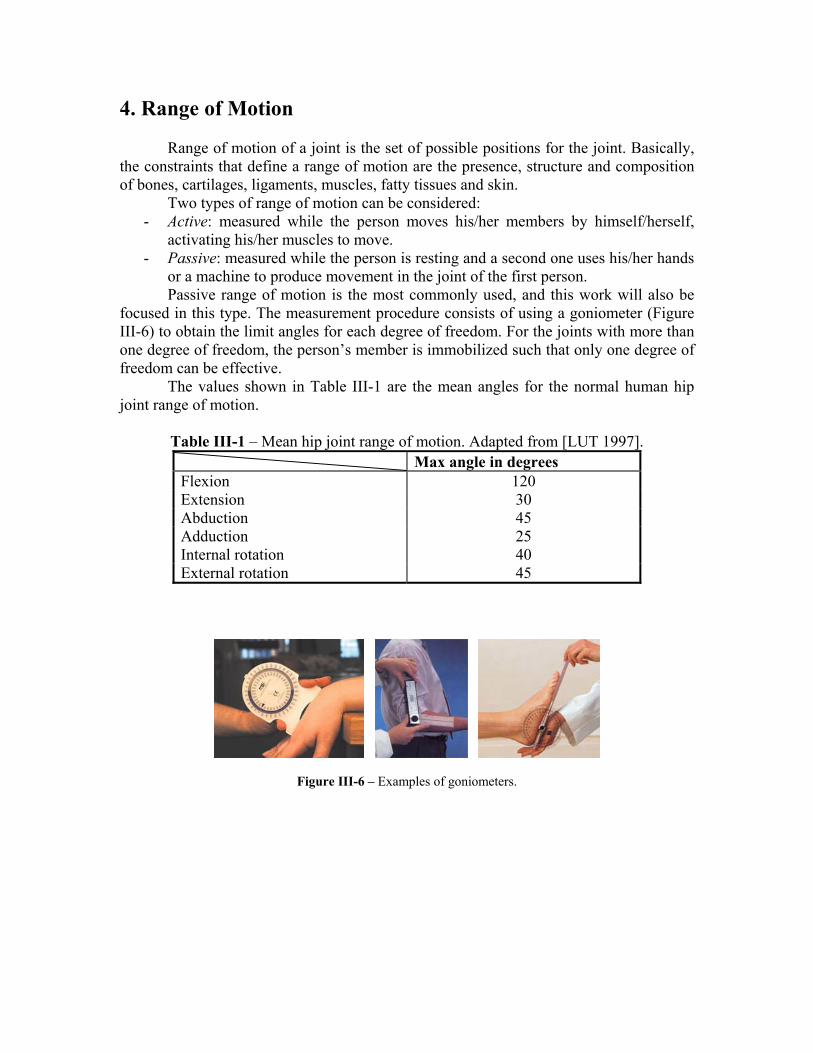
or a machine to produce movement in the joint of the first person. Passive range of motion is the most commonly used, and this work will also be

focused in this type. The measurement procedure consists of using a goniometer (Figure III-6) to obtain the limit angles for each degree of freedom. For the joints with more than one degree of freedom, the person’s member is immobilized such that only one degree of freedom can be effective.

The values shown in Table III-1 are the mean angles for the normal human hip joint range of motion.

Table III-1 – Mean hip joint range of motion. Adapted from [LUT 1997].

Max angle in degrees Flexion 120 Extension 30 Abduction 45 Adduction 25 Internal rotation 40 External rotation 45

Figure III-6 – Examples of goniometers.

IV. Conclusions Material Properties:

The enormous variations found in different human bodies cannot be attributed only to dimensions and structural proportions. The biomaterials compounding human tissues also considerably differ from one person to another. This affects the behavior of the tissues and consequently the way the body moves. The variations in tissue composition are not only a consequence of genetic heritage but are also a result of the physical stresses on the tissue during time and lifetime.

The human being is evolving along life and generations. In such evolution process, his body is constantly adapting itself to the functions it is demanded for. Through this functional adaptation process, the body of humans and other animals change its shape, composition and architecture such that it becomes suitable to develop its activities in the most optimal way. Thus, we are not surprised with the difficulty to find coherent values to biomaterials physical properties in the literature. Different research projects base their tests on tissue obtained from very different donators, what explains the variety of the available data. In this context, a work directed to model and simulate the behavior of a realistic human joint should relies in data obtained from a particular person, which real motion will be later used to validate the joint model. However, all these data are still very difficult to obtain. Hip Joint Components: Bones are responsible to transmit loads from one part of the body to another and are very rigid. Its deformation can only be observed in extreme situations of sports or accidents. So, in clinical use of a joint model, bones elasticity can be ignored without realism loss. Cartilage absorbs impacts and provides an excellent lubrication of the contacting surfaces of a joint. It is much softer than bones, but its thin layers are not significant for the external aspect of healthy joint motion. However, in pathological situations, any change in cartilage structure or composition is very important to both motion (specially range of motion) and sickness detection. Further, when a person rests several minutes in the same position, the cartilage deforms as a consequence of the stress on specific areas, and the deformation persists even some minutes after the person restarts moving due to its viscoelastic behavior. This causes abnormal behavior of the joint for some instants. Ligaments are usually structures that provide stability to the joint in different positions. Generally, ligaments are responsible in large extent to the range of motion of a joint, but in the specific case of the hip, it happens only in hyperextension. In fact, in this joint the ligaments basically work to keep the femur head inside the acetabular cup. Besides the well known mechanical resistance provided by this tissue in the other joints, in the hip capsule the ligaments create a kind of vacuum effect that increases several times the force necessary to dislocate the joint. A third and last structure of the hip (besides cartilage and ligament) that deserves special attention is the acetabular (or glenoidal) labrum, to which a description is already

done in the section about ligaments (III-2). In pathological cases, physical properties of the labrum change. It calcifies becoming harder (like bone), turn into a new impingement to the joint motion, and causes faster wear out of cartilage. So, it is imperative that real labrum material properties are considered in a realistic biomechanical model of the hip joint.

References [ABA 2002] Hibbitt, Karlsson & Sorensen, Inc. web site at: http://www.abaqus.com/ [AKE 1984] Akeson, W. H., Woo, S. L-Y., Amiel, D. and Frank, C.B. (1984). The

chemical basis of tissue repair. In L.Y. Hunter and F.J. Funk (Ed.) Rehabilitation of the Injured Knee (pp. 93-104). St. Louis: C.V. Mosby Company.

[ALG 2002] Algor Inc. web site at: http://www.algor.com/ [BEY 1996] P. Beylot et al. “3D Interactive Topological Modeling using Visible

Human Dataset.” NCC Blackwell, 1996. France. [BIOE 2002] “Articular Cartilage”. Rice University, Department of Bioengineering web

site at: http://www.ruf.rice.edu/~msbioe/hyaline.html [CAR 1999] William. F. CARROLL “A primer for finite elements in elastic

structures.” John Wiley & Sons Ltd., 1999. USA. [DES 1997] Mathiew DESBRUN “Modélisation et Animation de Matériaux

Heutement Déformables en Synthèse d'Images.” PhD Thesis. INP-Grenoble, 1997. France.

[DEL 1999] Hervé Delingette et al. “A Hybrid Elastic Model allowing Real-Time

Cutting, Deformations and Force-Feedback for Surgery Training and Simulation.” IEEE Computer Society, 1999. Switzerland.

[FER 2000] Stephen J. Ferguson. “Biomechanics of the Acetabular Labrum.” Queen’s

University. Phd Thesis. Kingston (Canada), 2000. [FIS 2000] Rebecca FISH. “Sinovial Joints.” Availavle at: http://www.teaching-

biomed.man.ac.uk/student_projects/2000/mmmr7rjf/articula.htm. University of Manchester, Department of Biological Sciences, 2000.

[FUN 1993] Y. C. FUNG “Biomechanics: mechanical properties of living tissues.”

Second Edition. Springer-Verlag, 1993. USA. [FUN 1972] Y. C. FUNG et al. (Eds.) “Biomechanics: Its Foundations and Objectives.”

Prentice-Hall Inc., 1972. USA. [GAL 1982] R. H. GALLAGHER et al. (Eds.) “Finite Elements in Biomechanics.”

John Wiley & Sons Ltd., 1982. USA.

[GRA 2000] Gray, Henry. Anatomy of the Human Body. Philadelphia: Lea & Febiger, 1918; Bartleby.com, 2000. “http://www.bartleby.com/107/". [Mar 18, 2002]

[HAW 2001] David HAWKINS “Tissue Mechanics.” Lecture available at:

http://dahweb.engr.ucdavis.edu/dahweb/126site/126site.htm. Human Performance Laboratory, University of California, Davis, 2001.

[INS 2001] Instron Corporation web site at: http://www.isntron.com [LUT 1997] Luttgens, K. & Hamilton, N. “Kinesiology: Scientific Basis of Human

Motion”. 9th Ed., Madison, WI: Brown & Benchmark, 1997. [MEN 1989] Menard, D. and Stanish, W.D. (1989). The aging athlete. American

Journal of Sports Medicine, 17(2), 187-196. [MER 1992] J. L. MERIAM & L. G. KRAIGE “Engineering Mechanics: Statics.” New

York: John Wiley & Sons, 1992. [MET 1997] Dimitri N. METAXAS “Physics-Based Deformable Models: Aplications

to Computer Vision, Graphics and Medical Imaging.” Kluwer Academic Publishers, 1997. USA.

[MOW 1997] Van C. MOW and Wilson C. HAYES “Basic Orthopaedic Biomechanics.”

Second Edition. Lippincott-Raven Publishers, 1997. USA. [MOW 1991] Van C. MOW et al. “Structure and Function of Articular Cartilage and

Meniscus”, Basic Orthopaedic Biomechanics, V.C. Mow and W.C. Hayes, Editors, Raven Press, New York, 1991.

[MTS 2001] MTS Systems Corporation web site at: http://www.mts.com [MYE 1983] Myers and Mow, “Cartilage: Structure, Function and Biochemistry”, v. 1,

ch.11, 1983. [NEB 2000] Jean-Cristophe NEBEL “Soft tissue modeling from 3D scanned data.”

MIRALab, 2000. Switzerland. [NIG 1994] B.M. NIGG and W. HERZOG (Eds.) “Biomechanics of the Musculo-

Skeletal System.” John Wiley & Sons Ltd., 1994. England. [SIM 1994] S. R. SIMONS. “Orthopaedic Basic Science.” Ed., AAOS, 1994 [WIN 1990] David A. WINTER “Biomechanics and Motor Control of Human

Movement.” Second Edition. Wiley-Interscience Publication, 1990. USA.

[WOO 1991] S. L. WOO et al. “Structure and Function of Tendons and Ligaments”, Basic Orthopaedic Biomechanics, V.C. Mow and W.C. Hayes, Editors, Raven Press, New York, 1991.

[WOO 1982] Woo, S. L-Y. Gomez, M.A., Woo, Y.K. and Akeson, W.H.: Mechanical

Properties of Tendons and Ligaments - II. The Relationships of Immobilization and Exercise on Tissue Remodeling. Biorhelogy, 19:397-408, 1982.

[ZIE 2000] O. C. Zienkiewicz and R. L. Taylor “The Finite Element Method.”

Volume 1: “The Basis”. Fifth Edition. Butterworth-Heinemann, 2000. UK.