
![Uncalibrated pulse contour derived stroke volume variation predicts[1]](https://static.fdocuments.in/doc/165x107/556b02c5d8b42a2a4f8b514c/uncalibrated-pulse-contour-derived-stroke-volume-variation-predicts1.jpg)


![Enforcing Consistency Constraints in Uncalibrated Multiple ...wojtek/papers/multiHomogr.pdf · Enforcing Consistency Constraints in Uncalibrated Multiple ... tection [25, 46] or enhanced](https://static.fdocuments.in/doc/165x107/5f0d905a7e708231d43afb29/enforcing-consistency-constraints-in-uncalibrated-multiple-wojtekpapersmultihomogrpdf.jpg)

Languages
Pages
Legal

High-quality Depth from Uncalibrated Small Motion Clip
Hyowon Ha† Sunghoon Im† Jaesik Park‡ Hae-Gon Jeon† In So Kweon††Korea Advanced Institute of Science and Technology ‡Intel Labs
Abstract
We propose a novel approach that generates a high-quality depth map from a set of images captured with asmall viewpoint variation, namely small motion clip. Asopposed to prior methods that recover scene geometry andcamera motions using pre-calibrated cameras, we intro-duce a self-calibrating bundle adjustment tailored for smallmotion. This allows our dense stereo algorithm to producea high-quality depth map for the user without the need forcamera calibration. In the dense matching, the distributionsof intensity profiles are analyzed to leverage the benefit ofhaving negligible intensity changes within the scene due tothe minuscule variation in viewpoint. The depth maps ob-tained by the proposed framework show accurate and ex-tremely fine structures that are unmatched by previous liter-ature under the same small motion configuration.
1. Introduction
Small motion in a hand-held camera commonly happens
when a user moves the device slightly to find a better photo-
graphic composition, or even when the user tries to hold the
camera steady before pressing the shutter. If we were able
to restore the geometry of the scene using the small motion
clip captured at that moment, it could be useful for a variety
of applications, such as synthetic refocusing or view syn-
thesis. Figure 1 shows an example of the small motion clip.
The averaged image of the entire sequence gives a sense of
how small the camera motion is.
In this paper, we propose an effective pipeline for depth
acquisition from a small motion clip. At the core of our
approach is the novel bundle adjustment scheme that is spe-
cially devised to be applied to the small motion case. Unlike
to prior approaches, our algorithm can jointly estimate the
intrinsic parameters and poses of the camera from a small
motion footage, which imbues the proposed method with
practicality and severs the need for camera calibration.
By virtue of reliably estimating the intrinsic and extrin-
sic camera parameters, a plane sweeping based dense stereo
matching algorithm can be directly applied to produce a
dense depth map in a unified framework. A notable benefit
������������� �������
��������� ����� �
������������ ���������� ������� ��
������������������ �����
��������������������������
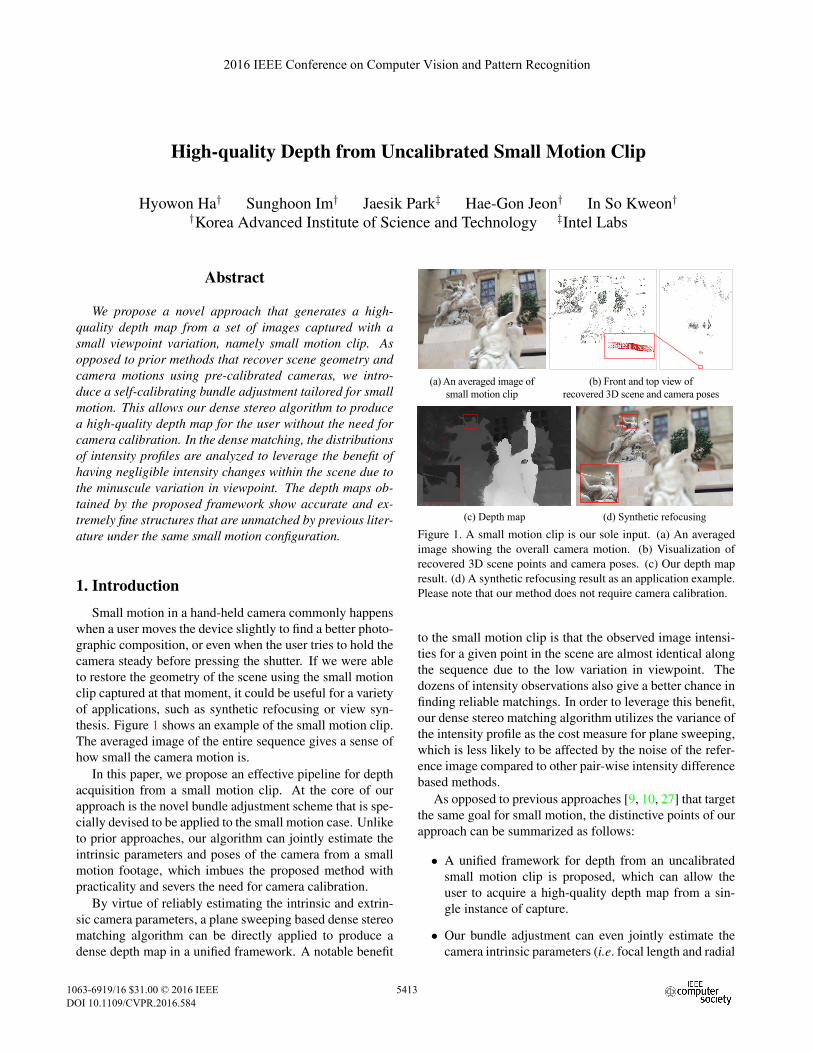
Figure 1. A small motion clip is our sole input. (a) An averaged
image showing the overall camera motion. (b) Visualization of
recovered 3D scene points and camera poses. (c) Our depth map
result. (d) A synthetic refocusing result as an application example.
Please note that our method does not require camera calibration.
to the small motion clip is that the observed image intensi-
ties for a given point in the scene are almost identical along
the sequence due to the low variation in viewpoint. The
dozens of intensity observations also give a better chance in
finding reliable matchings. In order to leverage this benefit,
our dense stereo matching algorithm utilizes the variance of
the intensity profile as the cost measure for plane sweeping,
which is less likely to be affected by the noise of the refer-
ence image compared to other pair-wise intensity difference
based methods.
As opposed to previous approaches [9, 10, 27] that target
the same goal for small motion, the distinctive points of our
approach can be summarized as follows:
• A unified framework for depth from an uncalibrated
small motion clip is proposed, which can allow the
user to acquire a high-quality depth map from a sin-
gle instance of capture.
• Our bundle adjustment can even jointly estimate thecamera intrinsic parameters (i.e. focal length and radial
2016 IEEE Conference on Computer Vision and Pattern Recognition
1063-6919/16 $31.00 © 2016 IEEE
DOI 10.1109/CVPR.2016.584
5413
distortion) as well as the camera poses and the scene
geometry from a single small motion clip.
• Our dense stereo matching that analyzes the intensityand gradient profiles in plane sweeping can generate
depth maps exhibiting extremely fine structures, which
have not been demonstrated in previous literature un-
der the same small motion conditions.
2. Related Work3D reconstruction from a hand-held camera is a widely
studied topic. SfM successfully recovers the sparse 3D ge-
ometry and camera poses for wide baseline images [7, 22].
The bundle adjustment [25, 4] minimizes the reprojec-
tion errors using an optimization framework. Other ap-
proaches [11, 21, 12] use the L∞ norm instead of the
L2 norm to make the cost function convex, but they are
more susceptible to outliers. As opposed to SfM, multi-
view stereo (MVS) can provide a depth for each pixel via
dense matching of the images [16]. Gallup et al. [5] presentan effective image matching method that selects a proper
baseline and image resolution adapted for the scene depth.
Conventional SfM and MVS approaches can reconstruct
accurate 3D geometry using wide-baseline images, but
users often cannot capture such images. Yu and Gallup [27]
propose an inspirational method that can estimate camera
trajectory even from a clip with hand-shaking motion. They
recover a dense depth map from a random depth initializa-
tion and perform a plane sweeping [3] based image match-
ing that incorporates a Markov Random Field [13]. Al-
though it is a well-known fact that narrow baselines affects
the accuracy of the estimated 3D geometry [17, 18, 19],
the inverse depth representation [27] is successfully demon-
strated in challenging small motion scenarios. Im et al. [9]extends [27] with the consideration of rolling the shutter
effect. Instead of performing dense image matching, they
propagates the tracked 3D points into the canonical image
domain. As the propagation is regularized by smooth sur-
face normal map obtained from sparse depth points, the re-
sulting depth map is also smooth. Joshi and Zitnick [10]
adopts a homography based image warping for dense im-
age matching with the micro baseline assumption. Their
algorithm even targets the tremble of a camera mounted on
a tripod.
The proposed approach also targets small motion clips
obtained by monocular cameras. To the best of our knowl-
edge, we are the first to demonstrate that even the camera
intrinsic and lens parameters can be reasonably estimated
from a small motion clip. This allows us to introduce a
fully automatic pipeline that performs a self-calibration of
the camera and estimation of a high-quality depth map. As
opposed to [27] that computes a pair-wise consistency be-
tween the images, our dense stereo measures the consis-
tency of the observed intensities by looking at the intensity
��������
��
������
��
������ �
i-th � �
�
� � �� �����������
���� ���
!�"������ ��
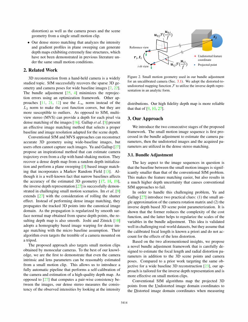
Figure 2. Small motion geometry used in our bundle adjustment
for an uncalibrated camera (Sec. 3.1). We adopt the distorted-to-
undistorted mapping function F to utilize the inverse depth repre-sentation in an analytic form.
distributions. Our high fidelity depth map is more reliable
that that of [9, 10, 27].
3. Our ApproachWe introduce the two consecutive stages of the proposed
framework. The small motion image sequence is first pro-
cessed in the bundle adjustment to estimate the camera pa-
rameters, then the undistorted images and the acquired pa-
rameters are utilized in the dense stereo matching.
3.1. Bundle Adjustment
The key aspect to the image sequences in question is
that the baseline between the small motion images is signif-
icantly smaller than that of the conventional SfM problem.
This makes the feature matching easier, but also results in
a much higher depth uncertainty that causes conventional
SfM approaches to fail.
In order to handle this challenging problem, Yu and
Gallup [27] introduce two practical clues: (1) the small an-
gle approximation of the camera rotation matrix and (2) the
inverse depth based 3D scene point parameterization. It is
shown that the former reduces the complexity of the cost
function, and the latter helps to regularize the scales of the
variables in the bundle adjustment. This idea is validated
well in challenging real-world datasets, but they assume that
the calibrated focal length is known a priori and do not ac-
count for the effects of the lens distortion.
Based on the two aforementioned insights, we propose
a novel bundle adjustment framework that is carefully de-
signed to estimate the focal length and radial distortion pa-
rameters in addition to the 3D scene points and camera
poses. Compared to a prior work targeting the same ob-
jective for a wide baseline 3D reconstruction [23], our ap-
proach is tailored for the inverse depth representation and is
more effective on small motion clips.
Conventional SfM algorithms map the projected 3D
points from the Undistorted image domain coordinates to
the Distorted image domain coordinates when measuring
5414
Front view Side view Top view
Yu and Gallup [27] (requires pre-calibration)
Our self-calibrating bundle adjustment
Reference view Our depth map
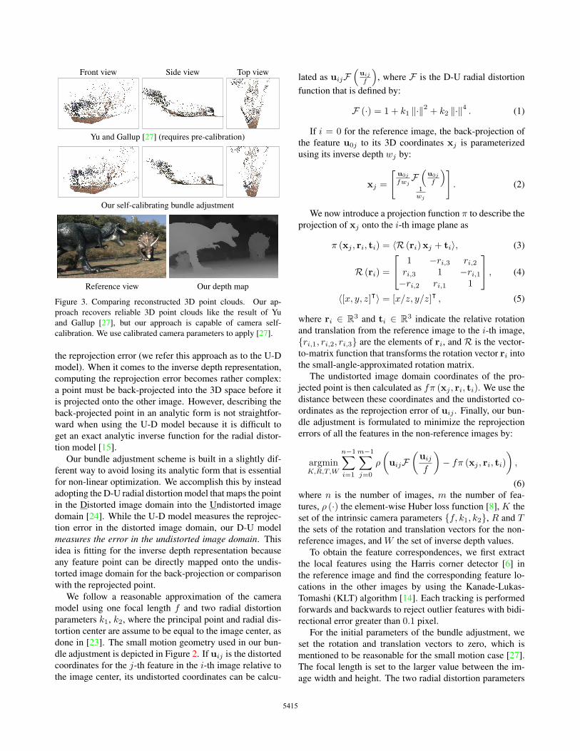
Figure 3. Comparing reconstructed 3D point clouds. Our ap-
proach recovers reliable 3D point clouds like the result of Yu
and Gallup [27], but our approach is capable of camera self-
calibration. We use calibrated camera parameters to apply [27].
the reprojection error (we refer this approach as to the U-D
model). When it comes to the inverse depth representation,
computing the reprojection error becomes rather complex:
a point must be back-projected into the 3D space before it
is projected onto the other image. However, describing the
back-projected point in an analytic form is not straightfor-
ward when using the U-D model because it is difficult to
get an exact analytic inverse function for the radial distor-
tion model [15].
Our bundle adjustment scheme is built in a slightly dif-
ferent way to avoid losing its analytic form that is essential
for non-linear optimization. We accomplish this by instead
adopting the D-U radial distortion model that maps the point
in the Distorted image domain into the Undistorted image
domain [24]. While the U-D model measures the reprojec-
tion error in the distorted image domain, our D-U model
measures the error in the undistorted image domain. Thisidea is fitting for the inverse depth representation because
any feature point can be directly mapped onto the undis-
torted image domain for the back-projection or comparison
with the reprojected point.
We follow a reasonable approximation of the camera
model using one focal length f and two radial distortionparameters k1, k2, where the principal point and radial dis-tortion center are assume to be equal to the image center, as
done in [23]. The small motion geometry used in our bun-
dle adjustment is depicted in Figure 2. If uij is the distorted
coordinates for the j-th feature in the i-th image relative tothe image center, its undistorted coordinates can be calcu-
lated as uijF(uij
f
), where F is the D-U radial distortion
function that is defined by:
F (·) = 1 + k1 ‖·‖2 + k2 ‖·‖4 . (1)
If i = 0 for the reference image, the back-projection ofthe feature u0j to its 3D coordinates xj is parameterized
using its inverse depth wj by:
xj =
[u0jfwj
F(u0jf
)1wj
]. (2)
We now introduce a projection function π to describe theprojection of xj onto the i-th image plane as
π (xj , ri, ti) = 〈R (ri)xj + ti〉, (3)
R (ri) =
⎡⎣ 1 −ri,3 ri,2
ri,3 1 −ri,1−ri,2 ri,1 1
⎤⎦ , (4)
〈[x, y, z]ᵀ〉 = [x/z, y/z]ᵀ, (5)
where ri ∈ R3 and ti ∈ R
3 indicate the relative rotation
and translation from the reference image to the i-th image,{ri,1, ri,2, ri,3} are the elements of ri, and R is the vector-
to-matrix function that transforms the rotation vector ri intothe small-angle-approximated rotation matrix.
The undistorted image domain coordinates of the pro-
jected point is then calculated as fπ (xj , ri, ti). We use thedistance between these coordinates and the undistorted co-
ordinates as the reprojection error of uij . Finally, our bun-
dle adjustment is formulated to minimize the reprojection
errors of all the features in the non-reference images by:
argminK,R,T,W
n−1∑i=1
m−1∑j=0
ρ
(uijF
(uij
f
)− fπ (xj , ri, ti)
),
(6)
where n is the number of images, m the number of fea-
tures, ρ (·) the element-wise Huber loss function [8],K the
set of the intrinsic camera parameters {f, k1, k2}, R and Tthe sets of the rotation and translation vectors for the non-
reference images, andW the set of inverse depth values.
To obtain the feature correspondences, we first extract
the local features using the Harris corner detector [6] in
the reference image and find the corresponding feature lo-
cations in the other images by using the Kanade-Lukas-
Tomashi (KLT) algorithm [14]. Each tracking is performed
forwards and backwards to reject outlier features with bidi-
rectional error greater than 0.1 pixel.For the initial parameters of the bundle adjustment, we
set the rotation and translation vectors to zero, which is
mentioned to be reasonable for the small motion case [27].
The focal length is set to the larger value between the im-
age width and height. The two radial distortion parameters
5415
��
��
��
��#�
!$
!%
!�
��� �������
!�� ������
���� ���� � ����
���
�� &�
������
�� ���
�� �����
�� ���
��� ������
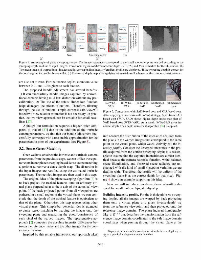
Figure 4. An example of plane sweeping stereo. The image sequences correspond to the small motion clip are warped according to the
sweeping depth. (a) One of input images. Three local regions of different scene depth – P1, P2, and P3 are marked for the illustration. (b)The mean image of warped input images and its corresponding intensity/gradient profile are displayed. If the sweeping depth is correct for
the local region, its profiles become flat. (c) Recovered depth map after applying winner-takes-all scheme on the computed cost volume.
are also set to zero. For the inverse depths, a random value
between 0.01 and 1.0 is given to each feature.The proposed bundle adjustment has several benefits:
1) It can successfully handle images captured by conven-
tional cameras having mild lens distortion without any pre-
calibration. 2) The use of the robust Huber loss function
helps disregard the effects of outliers. Therefore, filtering
through the use of random sample consensus (RANSAC)
based two view relation estimation is not necessary. In prac-
tice, the two view approach can be unstable for small base-
lines [27].
Although our formulation requires a higher order com-
pared to that of [27] due to the addition of the intrinsic
camera parameters, we find that our bundle adjustment suc-
cessfully converges with a reasonable approximation for the
parameters in most of our experiments (see Figure 3).
3.2. Dense Stereo Matching
Once we have obtained the intrinsic and extrinsic camera
parameters from the previous stage, we can utilize these pa-
rameters in our plane sweeping based dense stereo matching
algorithm to recover a dense depth map. The distortion in
the input images are rectified using the estimated intrinsic
parameters. The rectified images are then used in this step.
The original idea of the plane sweeping algorithm [3] is
to back-project the tracked features onto an arbitrary vir-
tual plane perpendicular to the z-axis of the canonical viewpoint. If the back-projected points from all viewpoints are
gathered in a small region of the virtual plane, we can con-
clude that the depth of the tracked feature is equivalent to
that of the plane. Otherwise, this step repeats using other
virtual planes. This simple but powerful idea is extended
to dense stereo matching by warping the images onto the
sweeping plane and measuring the photo consistency of
each pixel of the warped images. The representative ap-
proach [2] computes the absolute intensity differences be-
tween the reference image and the other images for the con-
sistency measure.
Inspired by this reliable framework, our approach takes
��������
� �
����'(�)
���
����'(�)
*��
������ ��)
���
������ ��)
*��
Figure 5. Comparison with SAD based cost and VAR based cost.
After applying winner-takes-all (WTA) strategy, depth from SAD
based cost (WTA-SAD) shows higher depth noise than that of
VAR based cost (WTA-VAR). As a result, WTA-SAD gives in-
correct depth when depth refinement algorithm [26] is applied.
into account the distribution of the intensities acquired from
the pixels in the warped images that correspond to the same
point on the virtual plane, which we collectively call the in-tensity profile. Consider the observed intensities in the pro-file acquired from the correct sweeping depth; it is reason-
able to assume that the captured intensities are almost iden-
tical because the camera response function, white-balance,
scene illumination, and observed scene radiance are un-
changed with the kind of small viewpoint variation we are
dealing with. Therefore, the profile will be uniform if the
sweeping plane is at the correct depth for that pixel. Fig-
ure 4 shows an example supporting this idea.
Now we will introduce our dense stereo algorithm de-
vised for small motion clips, step-by-step.
Building intensity profile. For the k-th depth in nk sweep-
ing depths, all the images are warped by back-projecting
them onto a virtual plane at a given inverse-depth1 wk
from the reference viewpoint, and then projected onto the
reference image domain. The plane-induced homography
Hik ∈ R3×3 that describes the transformation from the ref-erence image domain coordinates to the i-th image domaincoordinates when passing through the virtual plane at the
1To prevent the abuse of the notation, we view the inverse depth wk =1zkas a practical analog to the depth candidate.
5416

����' ��)��+�)��� ����,��� ������ ��������� ���� ���������* �
Figure 6. The sequential procedures to get the dense depth map. (a) Rough depth map acquired by applying winner-takes-all strategy on the
cost volume, (b) after the removal of unreliable depth pixels through our approach, and (c) after the depth refinement algorithm is applied.
(d) The reference image. Note the fine structures observable in the bicycles.
k-th sweeping depth can be formulated by:
Hik = K
⎡⎣ 1 −ri,3 ri,2 + wkti,1
ri,3 1 −ri,1 + wkti,2−ri,2 ri,1 1 + wkti,3
⎤⎦K−1, (7)
where {ti,1, ti,2, ti,3} are the elements of ti and K is de-
fined as[ f 0 pu
0 f pv
0 0 1
]. (pu, pv) in K is the principal point co-
ordinates equated to the image center. Using this homogra-
phy, the i-th undistorted image Iui can be warped into the
reference image domain through the operation described by
the following formulation:
Iik(u) = Iui (〈Hiku〉), (8)
where 〈·〉 is the same function defined in Eq. (5) and Iikis the warped i-th image according to the k-th sweepingdepth. After warping n images, every pixel u in the ref-erence image domain has an intensity profile P(u, wk) =[I0k(u), · · · , I(n−1)k(u)] for the inverse depth candidatewk.
Compute matching cost volume. Based on earlier discus-sions, we measure the consistency of the intensity profile to
evaluate the alignment of the warped images. Our match-
ing cost CI for pixel u and depth candidate wk is defined as
follows:
CI(u, wk) = VAR( [
I0k(u), · · · , I(n−1)k(u)] )
, (9)
where VAR(p) is the variance of vector p. In order to en-force the matching fidelity on the edge regions of the image,
we introduce two additional costs Cδu and Cδv defined as the
horizontal and vertical gradients of the images, respectively.
Cδu is defined as follows:
Cδu(u, wk) = VAR
([δI0kδu
(u), · · · , δI(n−1)kδu
(u)
]),
(10)
where δIδu indicates the image gradient in the horizontal di-
rection. We use the first-order gradient filter F = [−1 0 1 ]to approximate δI
δu in the discrete and finite image space.Cδv is similarly calculated using the vertical gradients ob-
tained by using Fᵀ. The comprehensive matching cost C isdefined as
C = CI + λ(Cδu + Cδv). (11)
Although the numerous intensity observations in the pro-
file give a reliable matching cost, the variance operator used
in Eq. (9) and (10) may not robustly compute the deviation
of the profile in the presence of outliers. The application of
a 3× 3 box filter on C can suppress some of the noise in thecosts. The proposed matching scheme is found to recover
the fine structures in the depth map results, which will be
shown later.
The proposed cost volume C is analogous to the conven-tional plane sweeping stereo [2], which computes the sum
of absolute intensity difference (SAD) between the refer-
ence image and the other images. Here, the notable dif-
ference to our method is that the pairwise matching costs
depend on the reference image; if the reference image in-
cludes a large amount of noise, the matching cost will be
less reliable. By contrast, our variance operator handles ev-
ery element equally. Figure 5 shows the depth map compar-
ison between the SAD based cost and the VAR based cost
after applying the winner-takes-all strategy and the succes-
sive refinement.
Depth refinement. After applying the winner-takes-all
strategy on the cost volume C, we get the depth map Dwin.
Although Dwin gives a reasonable depth estimate, some
values of Dwin can be noisy when homogeneous textures
are present in that region as may not give an obvious
cost minimum. To handle noisy depth, we define a con-
fidence measure described by the formulation M(u) =1−CI(u, Dwin(u))/P(u, Dwin(u)), where P is the mean
5417

-���������
����
00.20.40.60.81
-3.5 -3.1 -2.7 -2.3 -1.9 -1.50
0.20.40.60.81
2 6 10 14 18 22 26 30������.��� �/0 �1��������� �� #�������������� ��
2
%34
�=��
�=��
�=�
�=-�13
�=-�13
�=-�13
�� �3 �5 �$2 �� �3 �5 �$2
��� ��� ��� ���
2
%34
Figure 7. Synthetic experiments with respect to the magnitude of the baseline (n = 31) and the number of images (b = −2.1). (a), (c)Depth maps obtained by the proposed WTA and their difference maps. (b), (d) Robustness measure results denoting the percentage of
pixels within 3, 5, 7, and 10 label differences from the ground truth.
Algorithm 1: Depth from Small Motion Clip
Input: Image sequence {Ii}n−1i=0
Output: Depth mapDout
- Compute relative pose {ri, ti}n−1i=0 , 3D points {x} of the
scene, and lens parameters f , k1, k2 (Sec. 3.1)
- Undistort {Ii}n−1i=0 to get {Iui }n−1
i=0
- nk = number of label, zmin = nearest depth of xfor k = 1 : nk do
- Set wk = knkzmin
for i = 0 : (n− 1) do- Warp Iui using wk,K,Ri, and ti (Eq. (7))
- Build intensity/gradient profiles and compute cost
volume C (Eq. (9, 10, and 11))- Winner-takes-all on C and getDwin
- RefineDwin and getDout (Sec. 3.2)
of the intensity profile P used for normalizing the confi-
dence map scale. IfM(u) is smaller than a constant thresh-old, we declare them as outlier pixels. Dwin and M(u)are used for the depth refinement algorithm [26] that en-
forces smoothness on the depth image using the guidance
of the reference color image. [26] is based on the mini-
mum spanning tree structure, and it requires only 2 addi-
tion/subtraction operations and 3 multiplication operations
in total for each pixel. Figure 6 shows an example of the
outlier detection and the refinement. The overall pipeline of
our approach is summarized in Algorithm 1.
4. Experimental Results
4.1. Synthetic Dataset
We devise a synthetic experiment to analyze the algo-
rithm’s dependence on the magnitude of the baseline mo-
tion and on the number of images. We render 11 clips eachcontaining one reference image and 30 non-reference im-
ages all captured at a fixed distance around the z-axis of the
reference image. The baselines are determined relative to
the minimum depth of the scene from the reference image.
All the images are rendered using the BlenderTM software
at a set resolution of 640 × 480. Since our algorithm de-
R3 R5 R7 R10 MAD
SAD 43.331 64.940 78.337 86.419 8.650
VAR 44.349 67.728 81.646 90.201 5.763Table 1. Quantitative comparison between the SAD based cost and
VAR based cost using one of our synthetic clips (b = −2.1, n =31). MAD denotes the mean of absolute depth label difference.
termines the camera pose and scene depth up to a scaled
factor, the obtained depth map and the ground truth has to
be normalized into the same range, from 1 to 256 in our
case, for an accurate assessment. Fig. 7 shows the depth
map results obtained by the proposed WTA scheme and
their corresponding difference maps by varying magnitudes
of the baseline, shown in Fig. 7.(a), and the number of im-
ages used, Fig. 7.(c), respectively. Additionally, it shows
the results of the quantitative evaluations, Fig. 7.(b) and
Fig. 7.(d), using the robustness measure employed by the
Middlebury stereo evaluation system [20]; R5 denotes thepercentage of pixels that come within an absolute distance
of 5 labels from the ground truth label. These two evalua-
tions demonstrate that our method can produce a depth with
an R5 score of at around 80% as long as the magnitude of
the baseline is greater than 1% of the nearest scene depth
and the number of frames captured exceeds 30 frames. This
roughly equates to a 1 second small motion clip.
We also carried out a quantitative comparison by using
either the SAD based cost or the proposed VAR based cost
in the plane sweeping stage. In this experiment, the ground-
truth camera parameters of our synthetic clip (b = −2.1,n = 31) are given to the depth map acquisition pipeline. Asshown in Table 1, the WTA depth map using the SAD based
cost gives worse results than that of the VAR based cost.
The reason behind this result is that the SAD based cost is
easily affected by quality of the reference image, which may
contain noise, whereas the VAR based cost has no bias and
considers the importance of all input images equally.
4.2. Real-world Dataset
Camera setup. We have tested our method using a machinevision camera, Flea3 from Point Grey, Inc. (1280 × 960resolution at 30fps), and an iPhone 6 with two video modes
5418

Figure 8. Depth maps acquired by our algorithm. For each dataset, the left image shows the averaged image of the footage to indicate
the amount of camera movement, and the right image shows the estimated depth map using our algorithm. The clips are captured by a
hand-held iPhone 6 device using the default video capturing mode. Note that the capture times of the displayed clips are only one second.
Point Grey Flea3 iPhone6#1 (11) #2 (6) #1 (7) #2 (7)
Focallength
(pixel/scale) GT 1685.95 1685.02 1283.05 1293.73
Initial 1280.00 1280.00 1000.00 1000.00
Refined Min 1656.44 1634.14 1253.45 1279.52
Mean 1707.74 1684.74 1300.06 1301.56Max 1771.43 1748.79 1351.44 1332.44
Distortion
error(pixel)
Initial 5.76 5.89 3.65 3.25
Refined Min 0.09 0.02 0.89 0.97
Mean 0.52 0.53 1.48 1.14Max 1.26 1.20 2.17 1.49
Table 2. Evaluation on the estimated intrinsic camera parameters
(i.e. focal length and radial distortion). We have tested 31 clips(identified by the number in the parenthesis) grabbed by two cam-
eras with different lens settings. The ground truth camera parame-
ters (GT) are acquired using the camera calibration toolbox [28].
(1920 × 1280 at 30fps and 1280 × 720 at 240fps). For the240 fps videos, 30 frames are uniformly sampled from thefirst 240 frames. As the proposed method can utilize the fullresolution of the images, the estimated depth maps have the
same resolution as the inputs. The datasets are captured by
multiple users independent to this research. The small mo-
tion clips contain various types of motions, such as the one-
directional or waving motion. The maximum distances for
the captured scenes range from a wide variety of distances.
Figure 8 shows high-quality depth maps from various types
of small motions.
Computational time. In order to process each small mo-tion footage (30 frames of 1280 × 720 res. images), ourunoptimized implementation takes about one minute to per-
form feature extraction, tracking, and bundle adjustment.
We use the Ceres solver for the sparse non-linear optimiza-
tion [1]. The dense stereo matching stage takes about 10
minutes. The reported time is measured without CPU par-
allelization. We use a desktop computer equipped with an
Intel i7-4970K 4.0Ghz CPU and 16GB RAM. The data and
program are released on our project website.
Evaluation on the camera self-calibration. As the pro-posed bundle adjustment is designed to self-calibrate the
intrinsic camera parameters, we devise a quantitative evalu-
ation method for the camera parameters obtained by our ap-
proach. For this experiment, we use the calibrated Flea3 and
iPhone6 cameras, each while on two different lens settings2 .
Table 2 compares the estimated focal length and radial dis-
tortion against the ground truth. Here, we intentionally set
the initial focal length to be significantly different from the
ground truth. For measuring the distortion error, we gen-
erate a pixel grid and transform their coordinates using the
estimated D-U functionF . The transformed coordinates areagain applied with the ground-truth U-D model found in the
camera pre-calibration. If the estimated F is reliable, these
sequential transformation should be identity. The distortion
error is measured in pixels using the mean of absolute dis-
tances. The results show that the estimated parameters are
close to the ground truth. Notably, the mean distortion er-
ror from the Flea3 datasets is around 0.5 pixels, while theinitial parameter (k1,2 = 0) had an error of 5.8 pixels.
Comparison with [9, 27]. Figure 9 shows the depth mapsacquired by Yu and Gallup [27], Im et al. [9], and our ap-proach. We use the dataset and results provided by their
2iPhone can hold a fixed focal length if the user touches the region of
interest in the preview screen for a long time.
5419

Averaged image of the clips Yu and Gallup [27] Im et al. [9] Our results
Figure 9. Comparison with state-of-the-art approaches. The amount of camera movement is quite small as indicated by the averaged images
on the far left. The results of Yu and Gallup [27] show an inaccurate depth discontinuity on the shadow and indicate that the brick wall
is nearer than the ground. Our result shows a similar depth tendency to [9] while exhibiting much sharper depth discontinuities. The
erroneous region in our approach is also marked in red.
One of input images Our depth map
Joshi and Zitnick [10] Our synthetic refocusing
Figure 10. Comparison with Joshi and Zitnick [10] on the appli-
cation of synthetic refocusing. Our high-quality depth map gener-
ates an admirable foreground focused image from the small mo-
tion clip. Note that our result shows realistic defocus blurs on the
background whilst preserving sharp edges in the foreground (bot-
tom region of the cup).
respective websites for the pair comparison. The results
by [27] have inaccurate depth values as marked with the red
rectangles. The results of [9] show better depth values, in-
dicating that the ground plane is nearest to the camera. This
is due to their explicit consideration of the rolling shutter
effect. However, the depth discontinuity is too smooth, re-
sulting in blurry object boundaries unsuitable for the use of
synthetic refocusing. Our results have similar depth values
to [9] but show much sharper edge boundaries. Note that
our approach performs a self-calibration of the camera pa-
rameters for the displayed results, whereas [27, 9] utilize
the factory settings for the camera focal length and do not
account for the lens distortion.
Comparison with [10]. The synthetic refocusing image ob-tained by using our depth map is compared with that of [10].
We also use the dataset and result provided by [10] for the
pair comparison. As shown in Fig. 10, our foreground fo-
cused image consistently gives realistic defocus blurs.
Limitations. Although our algorithm is specially designedfor small baselines, the estimated camera poses become un-
reliable if the motion is unreasonably small. However, ac-
cording to Sec. 4.1, the required minimum baseline to apply
our approach is reasonable, and such failure cases rarely
happen in real hand-held scenarios. We observe that the
lack of features near the image border results in the erro-
neous estimation of the radial distortion parameters. Our
approach does not explicitly take into account the effects of
occlusion/dis-occlusion because the detected outliers in our
depth post-processing stage reasonably correspond to such
regions. However, any sophisticated occlusion inference al-
gorithm could be applied here.
5. ConclusionWe have introduced a practical algorithm that recovers a
high-quality depth map from a small motion clip recorded
by commercial cameras. Our self-calibrating bundle adjust-
ment estimates the camera parameters that are shown to be
close to the ground truth, even if only one second of the
clip is used. Our dense stereo matching step analyzes the
statistics of intensity profile and shows a superior depth map
than that of the previous approaches. In the future, we plan
to study the convergence properties of the proposed bundle
adjustment scheme.
Acknowledgement This work was supported by the National
Research Foundation of Korea (NRF) grant funded by the Korea
government (MSIP) (No.2010-0028680).
5420
References[1] S. Agarwal, K. Mierle, and Others. Ceres solver. http:
//ceres-solver.org.[2] A. Akbarzadeh, J. m. Frahm, P. Mordohai, C. Engels,
D. Gallup, P. Merrell, M. Phelps, S. Sinha, B. Talton,
L. Wang, Q. Yang, H. Stewenius, R. Yang, G. Welch,
H. Towles, D. Nistr, and M. Pollefeys. Towards urban 3d
reconstruction from video. In in 3DPVT, pages 1–8, 2006.[3] R. T. Collins. A space-sweep approach to true multi-image
matching. In Proceedings of IEEE Conference on Com-puter Vision and Pattern Recognition (CVPR), pages 358–363. IEEE, 1996.
[4] D. Crandall, A. Owens, N. Snavely, and D. Huttenlocher.
Discrete-continuous optimization for large-scale structure
from motion. In Proceedings of IEEE Conference on Com-puter Vision and Pattern Recognition (CVPR), pages 3001–3008. IEEE, 2011.
[5] D. Gallup, J.-M. Frahm, P. Mordohai, and M. Pollefeys.
Variable baseline/resolution stereo. In Proceedings of IEEEConference on Computer Vision and Pattern Recognition(CVPR), pages 1–8. IEEE, 2008.
[6] C. Harris and M. Stephens. A combined corner and edge
detector. In Alvey vision conference, volume 15, page 50,1988.
[7] R. Hartley and A. Zisserman. Multiple view geometry incomputer vision. Cambridge university press, 2003.
[8] P. J. Huber. Robust estimation of a location parameter. An-nals of Statistics, 53(1):73–101, 1964.
[9] S. Im, H. Ha, G. Choe, H.-G. Jeon, K. Joo, and I. S. Kweon.
High quality structure from small motion for rolling shut-
ter cameras. In Proceedings of International Conference onComputer Vision (ICCV), 2015.
[10] N. Joshi and C. L. Zitnick. Micro-baseline stereo. Tech-
nical report, Technical Report MSR-TR-2014-73, Microsoft
Research, 2014.
[11] F. Kahl. Multiple view geometry and the l-norm. In Pro-ceedings of International Conference on Computer Vision(ICCV), volume 2, pages 1002–1009. IEEE, 2005.
[12] F. Kahl, S. Agarwal, M. K. Chandraker, D. Kriegman, and
S. Belongie. Practical global optimization for multiview ge-
ometry. International Journal on Computer Vision (IJCV),79(3):271–284, 2008.
[13] P. Krahenbuhl and V. Koltun. Efficient inference in fully
connected crfs with gaussian edge potentials. arXiv preprintarXiv:1210.5644, 2012.
[14] B. D. Lucas and T. Kanade. An iterative image registra-
tion technique with an application to stereo vision. IJCAI,81:674–679, 1981.
[15] L. Ma, Y. Chen, and K. L. Moore. Rational radial distortion
models of camera lenses with analytical solution for distor-
tion correction. International Journal of Information Acqui-sition, 1(12):135–147, 2004.
[16] M. Okutomi and T. Kanade. A multiple-baseline stereo.
IEEE Transactions on Pattern Analysis and Machine Intel-ligence (PAMI), 15(4):353–363, 1993.
[17] J. Oliensis. Computing the camera heading from multiple
frames. In Proceedings of IEEE Conference on Computer
Vision and Pattern Recognition (CVPR), page 203. IEEE,1998.
[18] J. Oliensis. A multi-frame structure-from-motion algorithm
under perspective projection. International Journal on Com-puter Vision (IJCV), 34(2-3):163–192, 1999.
[19] J. Oliensis. The least-squares error for structure from in-
finitesimal motion. International Journal on Computer Vi-sion (IJCV), 61(3):259–299, 2005.
[20] D. Scharstein and R. Szeliski. A taxonomy and evaluation
of dense two-frame stereo correspondence algorithms. Inter-national Journal on Computer Vision (IJCV), 47(1-3):7–42,2002.
[21] K. Sim and R. Hartley. Recovering camera motion using
linfty minimization. In Proceedings of IEEE Conferenceon Computer Vision and Pattern Recognition (CVPR), vol-ume 1, pages 1230–1237. IEEE, 2006.
[22] N. Snavely, S. M. Seitz, and R. Szeliski. Photo tourism: Ex-
ploring photo collections in 3d. In Proceedings of ACM SIG-GRAPH, pages 835–846, New York, NY, USA, 2006. ACMPress.
[23] N. Snavely, S. M. Seitz, and R. Szeliski. Modeling the world
from Internet photo collections. International Journal ofComputer Vision, 80(2):189–210, November 2008.
[24] T. Tamaki, T. Yamamura, and N. Ohnishi. Unified approach
to image distortion. In Pattern Recognition (ICPR), 2002.Proceedings. 16th International Conference on, pages 584–587. IEEE, 2002.
[25] B. Triggs, P. F. McLauchlan, R. I. Hartley, and A. W. Fitzgib-
bon. Bundle adjustmenta modern synthesis. In Vision algo-rithms: theory and practice, pages 298–372. Springer, 2000.
[26] Q. Yang. A non-local cost aggregation method for stereo
matching. In Proceedings of IEEE Conference on ComputerVision and Pattern Recognition (CVPR), pages 1402–1409.IEEE, 2012.
[27] F. Yu and D. Gallup. 3d reconstruction from accidental
motion. In Proceedings of IEEE Conference on ComputerVision and Pattern Recognition (CVPR), pages 3986–3993.IEEE, 2014.
[28] Z. Zhang. A flexible new technique for camera calibration.
IEEE Transactions on Pattern Analysis and Machine Intelli-gence (PAMI), 22(11):1330–1334, 2000.
5421
Top Related