


Languages
Pages
Legal

Heat Transfer Enhancement Mechanisms in Parallel-Plate Fin Heat Exchangers
L. W. Zhang, S. Balachandar, D. K. Tafti, and F. M. Najjar
ACRC TR-93
For additional information:
Air Conditioning and Refrigeration Center University of Illinois Mechanical & Industrial Engineering Dept. 1206 West Green Street Urbana,IL 61801
(217) 333-3115
April 1996
Prepared as part of ACRC Project 38 An Experimental and Numerical Study of Flow
and Heat Transfer in Louvered-Fin Heat Exchangers S. Balachandar and A. M. Jacobi, Principal Investigators

The Air Conditioning and Refrigeration Center was founded in 1988 with a grant from the estate of Richard W. Kritzer, the founder of Peerless of America Inc. A State of Illinois Technology Challenge Grant helped build the laboratory facilities. The ACRC receives continuing supportfrom the Richard W. Kritzer Endowment and the National Science Foundation. The following organizations have also become sponsors of the Center.
Amana Refrigeration, Inc. Brazeway, Inc. Carrier Corporation Caterpillar, Inc. Dayton Thennal Products Delphi Harrison Thennal Systems Eaton Corporation Electric Power Research Institute Ford Motor Company Frigidaire Company General Electric Company Lennox International, Inc. Modine Manufacturing Co. Peerless of America, Inc. Redwood Microsystems, Inc. U. S. Anny CERL U. S. Environmental Protection Agency Whirlpool Corporation
For additional information:
Air Conditioning & Refrigeration Center Mechanical & Industrial Engineering Dept. University of Illinois 1206 West Green Street Urbana IL 61801
2173333115
HEAT TRANSFER ENHANCEMENT MECHANISMS IN PARALLEL-PLATE FIN HEAT EXCHANGERS
L. W. Zhang, Department of Mechanical & Industrial Engineering
S. Balachandar, Department of Theoretical & Applied Mechanics
D. K. Tafti, National Center for Supercomputing Applications
F. M. Najjar, National Center for Supercomputing Applications
University of Illinois at Urbana-Champaign
Urbana, IL 61801, U.S.A.
ABSTRACT
The heat transfer enhancement mechanisms and the performance of parallel-plate-fin heat ex
changers are studied using large scale direct numerical simulation. Geometry effects such as finite
fin thickness and fin arrangements (inline and staggered) have been investigated. The time-depen
dent flow behavior due to vortex shedding has been taken into consideration by solving the unsteady
Navier-Stokes and energy equations in two-dimensions. In the unsteady regime, in addition to the
time-dependent calculations, companion steady symmetrized flow calculations have also been per
formed to clearly identify the effect of vortex shedding on heat transfer and pressure drop. Addition
al comparisons have been made with the theoretical results for fully developed flow between unin
terrupted continuous parallel plates and that of restarted boundary layers with negligible fin
thickness [1], in order to quantify the role of boundary layer restart mechanism and the effect of finite
fin geometry.
INTRODUCTION
It has been known from simple theory and from empirical experimental results [1-9] that surface
interruption can be used for enhancing heat transfer. Some examples which exploit surface interrup
tion are the offset strip-fins and perforated-plate surfaces used widely in compact heat exchangers.
Surface interruption enhances heat transfer through two independent mechanisms. First, surface
interruption prevents the continuous growth of the thermal boundary layer by periodically interrupt
ing it. Thus the thicker thermal boundary layer in continuous plate-fins, which offer higher thermal
resistance to heat transfer, are maintained thin and their resistance to heat transfer is reduced. Pre
vious experimental and numerical studies have shown that this heat transfer enhancement mecha-
1

nism occurs even at low Reynolds numbers when the flow is steady and laminar [1, 2, 6]. Above
a critical Reynolds number, the interrupted surface offers an additional mechanism of heat transfer
enhancement by inducing self-sustained oscillations in the flow in the form of shed vortices. These
vortices enhance local heat transfer by continuously bringing fresh fluid towards the heat transfer
surfaces [10, 11].
In addition to heat transfer enhancement, surface interruption also increases the pressure drop
and thus requires higher pumping power. This is partly due to the higher skin friction associated
with the hydrodynamic boundary layer restarting. Also, in the unsteady regime, the time-dependent
flow behavior associated with vortex shedding increases form drag through Reynolds stresses [12,
13, 14]. Furthermore there are added losses through the Stokes layer dissipation [9]. Thus the
boundary layer restart and the self-sustained oscillatory mechanisms simultaneously influence both
the overall heat transfer and the pumping power requirement. Therefore design optimization must
take into account the impact of design parameters on the relative importance of the different heat
transfer enhancement mechanisms and their attendant effect on pumping cost.
Most theoretical and computational investigations of offset-strip-fin geometries [1, 2] have
often employed simplified models by assuming infinitesimally thin fins. By ignoring the finite
thickness of the fin, such models have suppressed periodic shedding of the vortices and thereby ac
count for only the boundary layer restart mechanism. Even studies which account for the finite fin
thickness [6, 15] have often assumed the flow to be symmetric about the wake centerline and thereby
obtained a stable laminar flow even at higher Reynolds numbers over the critical Reynolds number.
Thus many of the previous theoretical models and numerical simulations have precluded much of
the time-dependent flow physics and associated heat transfer enhancement and pumping power pen
alty though self-sustained oscillations.
With the rapid growth of computing power, large scale numerical simulations are becoming
more and more popular. It is now possible to obtain accurate time-dependent solutions with far few
er assumptions about the problem and to explore the full range of rich physics. For example, Ghad
dar et al. [8] and Amon and Mikic [9] have solved the unsteady incompressible Navier-Stokes and
energy equations using the spectral element method to study the unsteady flow and heat transfer in
communicating and grooved channels. These studies have shown that the flow physics associated
with flow separation at higher Reynolds numbers is too complex to be accounted for in steady state
computations.
In spite of these recent efforts, the details of the boundary layer restart and self-sustained oscilla
tory enhancement mechanisms have not been isolated and investigated in detail. In particular, in
the context of parallel plate-fin heat exchangers a clear understanding of the individual role of
boundary layer restart and the vortex shedding mechanisms on heat transfer and friction factor is
2
lacking. Flow visualizations have shown that vortices roll up near the leading edge of the flat fins
and subsequently travel downstream along the fin surface [16]. Von Karman vortices are also ob
served to form at the trailing edge of the flat fin and travel downstream in the wake before encounter
ing the next fin element. A number of important issues regarding how the vortices are generated
and how they interact with the parallel plate fins still remains to be explored. Although vortical
flows are considered to enhance overall heat transfer [10, 11] their impact on local heat transfer and
skin friction needs to be quantified. Similarly the effect of wake vortex shedding on form drag needs
to be quantified as well. Furthermore, the rate at which the strength of the leading edge vortex de
creases as it travels over the fin surface is unclear, but such understanding will have significant im
pact on design parameters such as fin length and fin thickness.
The primary objective of the present study is to first isolate the individual mechanisms through
controlled numerical simulations in parallel plate fin geometry. At higher Reynolds numbers when
the flow is naturally unsteady, along with the time-dependent simulations, corresponding steady
state simulations are performed as well, by artificially enforcing symmetry about the wake center
line. The difference between the unsteady and steady symmetrized simulation results are used in
exploring the unsteady enhancement mechanisms. These results are compared with the theoretical
results for fully developed flow between uninterrupted continuous parallel plates and those of re
started boundary layers with negligible fin thickness [1] to further separate the role of boundary layer
restart mechanism and the geometry effect in terms of finite fin thickness and fin arrangement. Two
different arrangements of the parallel plate fin geometry, inline and staggered (see Figure 1.) are
investigated over a range of Reynolds numbers.
MATHEMATICAL FORMULATION & PRELIMINARIES
In the present study we consider both inline and staggered parallel flat fin arrangements which
are shown in Figure 1. In the inline arrangement flat-fins of thickness, b, and length, L, form a peri
odic pattern with pitches Lx along the flow direction, x, and Ly=2H along the transverse direction,
y. Thus the basic unit, indicated by the dashed line, contains a single fin. Here we consider a large
periodic array of this basic unit periodically repeated along the streamwise and transverse directions
and Figure l(a) shows only six basic units of this large array. Figure l(b) shows the Staggered ar
rangement, where the basic unit which now contains two fin elements, again marked by the dashed
line, is periodically repeated along the streamwise and transverse directions. Staggered is the most
common arrangement investigated in the past due to its relevance to offset-strip-fins and it differs
from the inline arrangement in that the fin pitch in transverse direction is doubled. In the above two
cases the heat transfer surface area per unit volume is maintained the same and the actual sizes and
lengths employed in the simulations are given in terms of H.
3
The numerical simulations will assume periodicity of the velocity and temperature fields along
both the streamwise and transverse directions, over one basic unit and therefore the actual computa
tion geometry will be limited to this basic periodic unit. Thus, in an attempt to model the flow and
heat transfer in a large periodic array of fin elements, the present computations ignore the entrance
effects. Furthermore, the possibility of periodicity of the flow and thermal fields over multiples of
the basic unit along both the streamwise and transverse directions is ignored. This subharmonic ef
fects can be taken into account by employing a larger computational domain, which includes multi
ple elemental units, Mx and My respectively, along the x and y directions and assuming periodicity
of the flow and temperature fields over this extended domain. Through detailed computations in
communicating and grooved channels Amon [17] has shown that such subharmonic effects are small
in domains of large ratio of L.xIH, as the ones to be considered in this study. Therefore for the sake
of computational efficiency here we choose Mx=My=1.
The governing equations solved in two-dimensions for the non-dimensional velocity, u, and
temperature, T, fields are the N avier-Stokes equations along with the incompressibility condition
and the energy equation, as shown below:
au + u'\lu = e - \lp + _1_\l2u at x Rer inD (1)
aT + u,VT = 1 V2T at RerPr
inD (2)
\l·u = 0 inD (3)
where D denotes the computational domain, indicated by the dashed line in Figure 1 for each of the
two cases. In the above equations, the length and pressure scales are given by the half distance be
tween adjacent fin rows along the transverse direction, H, and the applied pressure difference over
a unit non-dimensional length along the streamwise direction, M. The corresponding velocity and
time scales are then given by (M/Q) 112 and (WQ/l'1p) 112, where Q is the density of the fluid. The
temperature has been nondimensionalized by q"H/k, where q" is the specified constant heat flux
on fin surfaces and k is the thermal conductivity of the fluid. Furthermore, to enable periodicity of
the flow field along the streamwise direction, the non-dimensional pressure gradient has been bro-
ken into an imposed constant mean streamwise pressure gradient given by the unit vector, ex, and
a fluctuating part, p, which can be considered periodic along x and y. Thus, in the present computa
tions the streamwise pressure gradient is maintained a constant and therefore the flow rate, Q, fluctu
ates over time, but for all the cases considered the flow rate fluctuation is less than 1 % of its mean
value.
Here we consider a constant heat flux boundary and under this condition, a modified temperature
field, e, can be defined as: e(x,y,t) = T(x,y,t) - yx, where y is the mean temperature gradient
4
along the flow direction. From a balance of the total rate of heat flux across the fin surface to the
fluid, y can be computed from the following expression: y Lx = g> / (Q ReT Pr), where g> is the perim-
eter of the fin surface in the x-y plane. The modified temperature, (), can then be considered as the
perturbation away from a linear temperature variation that accounts for the mean temperature varia
tion. Therefore () can be considered to be periodic along both x and y directions. Since the temporal
fluctuations in the flow rate are small, the corresponding fluctuations in yare also small in magni-
tude. On the surface of the fin, no-slip and no-penetration conditions are imposed for the velocity
field. The corresponding boundary condition for the modified temperature is given by
"() A A A (v )on = 1 - yexon on aDfin (4)
where Ii is the outward normal to the fin surface denoted by aDfin-
The numerical approach followed here is the direct numerical simulation where the governing
equations are solved faithfully with all the relevant length and time scales adequately resolved and
no models are employed. A second-order accurate Harlow-Welch scheme [18] is employed with
a control-volume formulation on a staggered grid with central difference approximations for the
convection terms. The equations are integrated explicitly in time until a steady or periodic or a statis
tically stationary state is reached. For the inline fin arrangement, the periodic domain with one fin
element is resolved with a grid of 128x32 grid cells. While in the staggered arrangement, the period
ic domain with two fin elements is discretized with 256x64 grid cells. A complete grid independence
study was conducted and showed satisfactory convergence of the solution [19]. A detailed descrip
tion of the numerical methodology can be found in Zhang et al. [19] and Tafti [20].
Before the presentation of the results the following quantities will be defined first. Although
the computations were performed with Hand (M/(}) 112 as the length and velocity scales, in the re
sults to be presented the Reynolds number, Re, is defined based on the hydraulic diameter, Dh, as:
VDh Re =-v and (5)
where Am is the minimum flow cross-section area, V is the average velocity at this section and A is
the heat transfer surface area. For both the arrangements shown in Figure 1 the minimum flow cross
sectional area is chosen to be (2H - b)Wand the heat transfer surface area is 2(b + l)W, where W
is the width of the fin in the spanwise, Z, direction, taken to be unity in the present two-dimensional
simulations. Local heat transfer effectiveness will be expressed in terms of the instantaneous local
Nusselt number based on hydraulic diameter is defined as:
Nu(s,t) = kdT/Dh
q" H [(}fs, t)-8 refs, t)]
(6)
5

where s measures the length along the periphery of the fin and the local reference temperature is
defined as () refs, t) = f ()Iuldy / f luldy. Here the absolute value of streamwise velocity is used so
that the regions with reverse flow are also properly represented [6]. Following the above definition,
the instantaneous global Nusselt number, <Nu(t», can be obtained through an integration around
the fin surface, Qf as:
< Nu > (t) = __ Q.::....f_D_h_1 H __
I(Or 0,<;,) tis
(7)
The overall Nusselt number, denoted by <Nu>, is then defined as the average of the above over time.
In order to evaluate the overall local heat transfer effectiveness we also define the time averaged
local Nusselt number, Nu(s), based on time averaged flow and thermal fields, u and (fin equations
6 and 7. In order to evaluate the overall performance of the system, the Colburn) factor which mea
sures heat transfer efficiency is defined as:
. <Nu> ] = RePrn
(8)
where n=OA for developed flow. And the friction factorfwhich measures the dimensionless pres
sure drop, is also defined here as:
f = 1.1:1') ~~) -(}v-2
RESULTS AND DISCUSSION
(9)
We begin by showing the various transitions undergone by the flow as the Reynolds number is
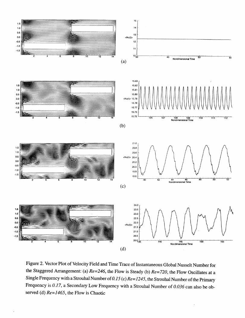
increased in geometries such as the inline and staggered arrangement of fins. Figure 2 shows the
flow pattern and the corresponding time variation of the instantaneous global Nusselt number for
the staggered geometry at four different Reynolds numbers: Re=246, 720, 1245 and 1465. The con
stancy of <Nu( t» indicates that the flow is steady laminar at Re=246. The recirculating bubble seen
in the wake is observed to grow in size with increasing Reynolds number in this steady regime. The
flow undergoes Hopfbifurcation at a critical Reynolds number somewhere between 474 and the next
higher Reynolds number of 720, which is consistent with Joshi & Webb [16] 's theoretical prediction
of Recrit = 688 for this geometry. Above this critical Reynolds number a time periodic state is ob
tained as can be inferred from the asymmetric state of the wake bubble and the small amplitude wavi
ness of the wake at Re=720. At this Reynolds number the time trace of the instantaneous global Nus
selt number shows that the flow oscillates at a single frequency, with a Strouhal number of 0.15,
6
where F is the primary frequency of oscillation. As Reynolds number further increases the flow
undergoes another instability as can be seen from the appearance of a strong secondary low frequen
cy in the plot Nusselt number at Re=1245. At this Reynolds number the Strouhal number of the pri
mary frequency increases to 0.17 and the Strouhal number for the secondary low frequency is 0.036.
Also can be seen is the appearance of well defined vortices that roll on the top and bottom surfaces
of the fin. With further increase in Reynolds number the flow soon becomes chaotic as shown by
the flow field and the Nusselt number at Re=1465.
The flow in the in line arrangement follows a similar qualitative pattern, although the transition
Reynolds number for the appearance of the various flow regimes quantitatively differs from those
of the staggered arrangement. In the inline arrangement, the flow remains steady for Reynolds num
bers under approximately 350. Above this, up to a Reynolds number of about 2000, the flow is ob
served to be unsteady with a single shedding frequency. The appearance of an additional frequency
and subsequent transitions to a chaotic state are delayed to higher Reynolds numbers. The primary
shedding frequency, F, nondimensionalized as, St = F b/V, for both the inline and staggered ar-
rangements are listed in Tables I and II, respectively. In both cases, the Strouhal number, St, can
be seen to be nearly a constant over a range of Reynolds number and jump to a higher value at higher
Re. By analyzing the Fourier transform of the velocity field along the streamwise direction, it was
confirmed that this jump is due to a discrete change in the number of waves that can be accommo
dated along the streamwise periodic domain. For the inline geometry, over the lower range of Re
ynolds number four waves were observed over a length of Lx and above a Reynolds number of 1400
five waves were observed. But the impact of the number of discretized waves on j and f factors at
any given Re was not observed to be strong. Although interesting this phenomenon will not be fur
ther pursued here.
It must be pointed out that the flow and thermal fields in the unsteady regime are qualitatively
similar in both the inline and staggered arrangements. For example Figure 3 shows the instantaneous
temperature contour for the staggered arrangement at Re=1465 and the corresponding velocity vec
tor field can be seen in Figure 2( d). Figure 4 shows the flow and thermal fields for the inline arrange
ment at a comparable Reynolds number of 1407. From these figures it is clear that in both these
arrangements there are vortices that roll on the top and bottom surfaces of the fin which significantly
alter the local thermal field and thereby the local heat transfer. These vortices are clockwise rotating
on the top surface and are anticlockwise rotating on the bottom surface. They act as large scale mix
ers and bring in cold fluid on their downstream side towards the fin surface. This can be seen to result
in the crowding of the temperature contours near the fin surface. The oscillatory nature of the flow
manifests itself in the wake of the fin elements as wavy motion that propagates in the streamwise
direction over time.
7
Global Results
In order to validate the present numerical approach in Figure 5 we compare the computedj and
jfactors for the staggered arrangement with experimental measurements on a corresponding offset
strip-fin geometry by Mullisen & Loehrke [21], numerical results of Patankar & Prakash [6] and
with correlations given by Joshi & Webb [16] and Manglik & Bergles [22]. Reasonable comparison
is obtained in both the heat transfer and pumping power results. In evaluating this comparison of
results it must be stated that while the current simulations and those ofPatankar & Prakash employed
a constant thermal flux boundary condition, the experiments modelled the isothermal condition.
Furthermore, the numerical simulations assumed periodicity along the streamwise direction and
thereby neglected the entrance and exit effects. In comparison to the geometric parameters
employed in the present simulations shown in Figure 1, Mullisen & Loehrke data are for LlH=4.55,
LxIH=9.10 andbIH=O.20 and the simulations ofPatankar & Prakash employed LlH=1 ,LxIH=2 and
blH=O.20. Three-dimensional effects were ignored in the current and Patankar & Prakash [6]'s sim
ulations. This effect is estimated to be small for the Mullisen & Loehrke [21]'s results presented
here, since the aspect ratio for this case is so small that it can be considered two-dimensional. In
plotting the results of Joshi & Webb and Manglik & Bergles, correlations corresponding to their
smallest aspect ratio (CIW) experiments is chosen in order to better approximate two-dimensionali
ty. Similar comparisons have also been performed for the inline geometry with the experimental
results of Mullisen & Loehrke [21] and they favorably agree with each other Zhang et al. [19].
In Figure 6 the Colbumj factor and the friction factor,f, are plotted againstRe on a log-log scale
for the staggered arrangement. Here the objective is to compare these results with those of Sparrow
& Liu [1] and those for continuous parallel plates to isolate contributions to heat transfer and friction
factor from the individual mechanisms. In order to make a fair comparison and proper estimation
of the individual effects it is important to follow a uniform scaling of all the results. The theoretical
results for the continuous flat plate, shown in figure as the solid line, are based on a fully developed
laminar flow and thermal fields between two infinitely long parallel plates with separation 4H. This
separation was chosen in order to maintain the heat transfer surface area per volume to be the same
as the inline or staggered arrangement. The Nusselt number and the friction factor, based on half
channel height, for a fully developed flow between parallel plates with constant heat flux are 35117
and 1.5IRe, respectively. For proper comparison, these when scaled to the hydraulic diameter defini
tion of the inline and staggered arrangements result in the followingj andjfactor relations
j = 5.94Re-1 and j = 9.38 Re-1 [Continuous Parallel Plates] (10)
where Re is the Reynolds number for the parallel plates based on the hydraulic diameter. In the limit
of flow between the continuous parallel plates boundary layer restart and vortex shedding mecha-
8
nisms are absent, as well as the geometry effect arising from the finite thickness and the placement
of the fin elements is ignored. These three effects together account for the substantial increase in
the j and f factors.
Also plotted as the dashed line in Figure 6 are the results obtained by Sparrow & Liu [1] for a
simplified model of the offset-strip-fin geometry. Once again, in order to maintain the heat transfer
area the same, the transverse spacing between fin rows is maintained 2H and the fin length is half
the computational domain C4/2). In their model the above two are the only parameters needed since
it was assumed that the fins are infinitesimally thin and the resulting flow is considered to be steady.
Their results on the j and f factors can be fit by a power law of the form:
j = 4.07Re- o.79 and f = 6.95 Re -0.82 [Sparrow & Liu] (11)
Therefore the difference between the continuous parallel plate and Sparrow & Liu's results accounts
for only the effect of periodically restarting the momentum and thermal boundary layers. It is clear
that the effect of boundary layer restart mechanism is to increase overall heat transfer but with the
associated penalty of higher frictional loss.
It is still difficult to fully assess the importance of self-sustained flow oscillations because the
difference between the present simulation results and those of Sparrow & Liu [1] also has contribu
tion from the geometry effect, mainly arising from the finite thickness of the fin. In order to further
isolate and separate these mechanisms, simulations were conducted in the same staggered arrange
ment shown in Figure 1, but with appropriate symmetry imposed about the wake centerline. Even
symmetry is enforced on u and e, while odd symmetry is enforced on v about the wake centerline.
This symmetrization of the flow removes all asymmetry in the wake associated with the shedding
process and thus the flow is constrained to follow the steady solution. We shall call these symme
trized simulations as "steady symmetrized simulations". It can be seen that the steady symmetrized
simulation also follows a power law behavior best fit by
j = 6.0 Re -0.84 and f = 6.2 Re -0.74 [Steady Symmetrized Staggered] (12)
Differences in the j and f factors of the steady symmetrized simulations and those of Sparrow & Liu
[1] account for the finite thickness of the fin elements and the resulting steady wake bubble.
The finite thickness of the fin does seem to affect the overall heat transfer behavior a little, pri
marily due to the fact that the finite fin thickness decreases the lateral spacing available for the flow
(C in Figure Ib) from 4H to 4H-b. If this change in the lateral spacing is accounted for then the
difference between the j factor of the steady symmetrized simulations and those of Sparrow and Liu
[1] is negligible. This suggests that the other effects of finite fin thickness can be ignored in heat
transfer considerations, at least over the Reynolds number range considered here. Similarly, the de
crease in lateral spacing available for the flow in the case of finite fin thickness accounts for most
of the increase in the f factor in the steady symmetrized simulations over the results of Sparrow &
9

Liu [1]. With this change in lateral spacing accounted for a noticeable increase in the friction factor
can be observed. This increase can be attributed to the contribution to friction factor arising from
the form drag, in case of finite fin thickness.
The full simulations are identical to the symmetrized steady simulations in the steady flow re
gime at low Reynolds numbers and follow the power law behavior. But above the critical Reynolds
number, once the flow becomes time-dependent, the full simulation results show systematic devi
ations from the power law with significant increase in both the j and f factors. Differences in the
performance of the steady symmetrized and the unsymmetrized full simulations is solely due to the
effect of flow oscillations.
Figure 7 shows the corresponding results for the inline fin arrangement. Here again a compari
son of the j and f factors from the continuous parallel plate theory, simulations of Sparrow & Liu
[1] for inline plates of infinitesimal thickness, steady symmetrized simulations and the full unsteady
simulations help to separate the individual contributions from the boundary layer restart, finite ge
ometry and self-sustained oscillatory effects. The results of Sparrow & Liu [1] and steady symme
trized simulations can be fit by the following power laws:
j = 6.03 Re-O·85 and f = 12.78 Re-O·89 [Sparrow & Liu] (13)
j = 10.5 Re- O.88 and f = 22.5 Re-O.82 [Steady Symmetrized InUne] (14)
The general trend seems to fit the description provided for the staggered arrangement. But there are
some differences. Mainly, the geometry effect given by the difference between the steady symme
trized simulations and the results of Sparrow & Liu [1] appears larger than the staggered counterpart.
This is because, in the inline geometry the effect of finite fin thickness in decreasing the lateral gap
available for the flow from 2H to 2H-b accounts for a 37.5% reduction in the flow cross-section.
Whereas, in the staggered arrangement the reduction in flow cross-section is only 18.75%. This de
crease in the flow cross section almost entirely accounts for the increase in j factor, but the f factor
is further increased by the presence of form drag in the case of finite fin thickness. Furthermore,
in both the inline and staggered arrangements, the fully developed boundary layer results can be seen
to slowly diverge off from the other two power laws with increasing Reynolds number. This effect
is more visible in the f factor. This is possibly due to the fact that at lower Reynolds numbers the
flow between the parallel plate fins rapidly develop into a fully developed flow, whereas as Re in
creases the entrance length for flow and thermal development also increases, thus increasing the
deviation from a fully developed flow. This hypothesis will later be confirmed with a careful look
at the hydrodynamic and thermal boundary layers.
A comparison of Figures 6 and 7 shows that for the same Reynolds number based on hydraulic
diameter, the inline arrangement results in a higher heat transfer accompanied by higher pumping
power than the staggered arrangement.
10

Local Nusselt Number Distribution
In the following, the role of the vortices in enhancing the local heat transfer will be closely ex
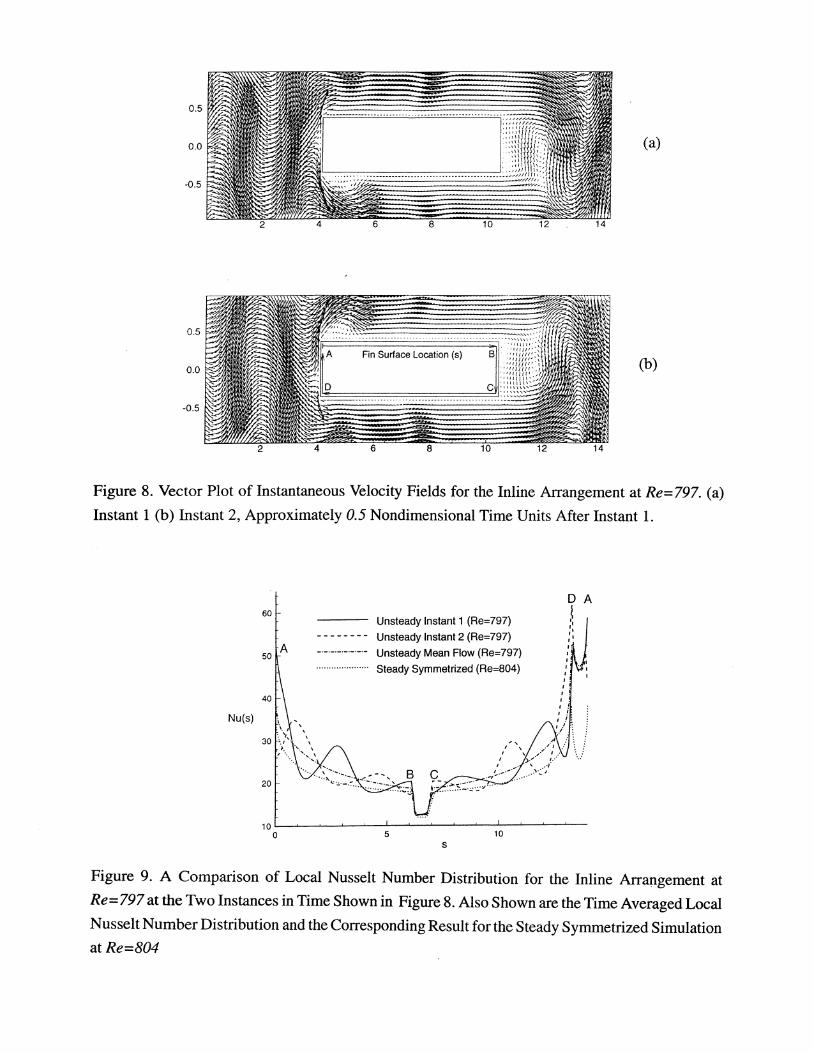
amined. Figure 8 shows the velocity vector field in the inline arrangement at Re=797 at two different
time instances. These two instances are separated by 0.5 nondimensional time units, which corre
sponds to 0.45 shedding periods. At the first time instance shown in Figure 8(a) an anticlockwise
vortex can be clearly seen to be located on the bottom left hand side of the fin. Over time this vortex
travels down the fin surface and at the later time instance shown in Figure 8(b) it has significantly
lost its strength and can be barely located at approximately x=7 on the bottom surface. In the mean
time a clockwise has been shed off the front top leading edge of the fin and can be seen to be located
at x=5. In fact the imprint of an earlier clockwise vortex can be seen in Figure 8( a) at x=8 as the inrush
of fluid towards the wall. Also marked in this figure are the fin surface locators starting from the
top left comer (Marked A) going around the fin clockwise (Marked B, C, D) and back to the top left
comer of the fin.
Figure 9 shows the instantaneous local Nusselt number, Nu(s,t), plotted around the fin periphery
at the two time instances shown in Figure 8. The local heat transfer efficiency is significantly large
at the leading edge due to the stagnation point nature of the flow, while the heat transfer efficiency
is significantly lower in the wake owing to the local recirculation. Enhancement in the local Nusselt
number can be well correlated with the presence of clockwise and anticlockwise vortices pointed
out in Figure 8. For example the anticlockwise vortex seen in Figure 8( a) at x=5 can be seen to gener
ate a strong local peak in the Nusselt number at s=12.2. At the later instance, this vortex has moved
downstream to s=8.2 and its impact on local Nusselt number has decreased. Similarly the clockwise
vortex on the top surface of the fin can also related to a bump in the Nusselt number variation and
it can be inferred that the vortices can increase local Nusselt number by as much as 50%.
Also plotted in this figure are the time-averaged local Nusselt number, Nu(s), for the unsteady
simulation and the local Nusselt number obtained from the corresponding steady symmetrized simu
lation at approximately the same Reynolds number (Re=804). In the case of the steady symmetrized
solution the monotonic decrease in the Nusselt number away from the front leading edge is solely
due to the growth in the thermal boundary layer. In the case of time-dependent simulations, signifi
cant improvement in the local heat transfer efficiency can be attributed to the presence of vortices.
The vortices can be seen to adversely affect local Nusselt number on their upstream end where fluid
is pushed away from the fin surface and result in a local decrease in the Nusselt number below the
steady symmetrized simulation result. On the other hand, a huge increase in the local Nusselt num
ber is realized at the downstream side of the vortex where fluid is brought to the fin surface, which
more than compensate for the decrease at the other upstream end. The net effect is to increase heat
11
transfer over the entire fin surface in the time-dependent flow regime. The rapid fall in the local
Nusselt number in the unsteady simulations is both due to the growth of the thermal boundary layer
and due to the decrease in the strength of the vortices.
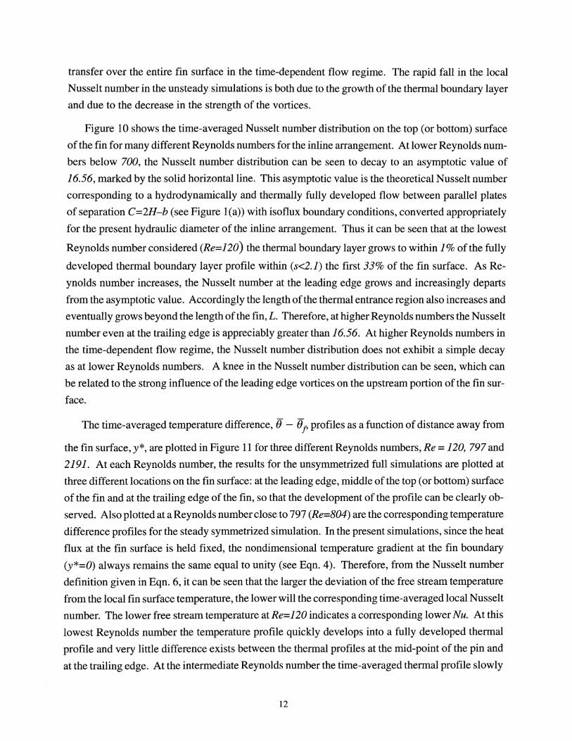
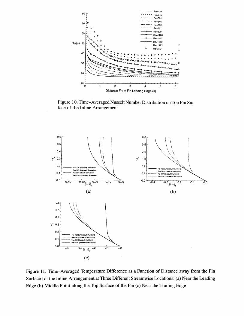
Figure 10 shows the time-averaged Nusselt number distribution on the top (or bottom) surface
of the fin for many different Reynolds numbers for the inline arrangement. At lower Reynolds num
bers below 700, the Nusselt number distribution can be seen to decay to an asymptotic value of
16.56, marked by the solid horizontal line. This asymptotic value is the theoretical Nusselt number
corresponding to a hydrodynamically and thermally fully developed flow between parallel plates
of separation C=2H-b (see Figure 1 (a» with isoflux boundary conditions, converted appropriately
for the present hydraulic diameter of the inline arrangement. Thus it can be seen that at the lowest
Reynolds number considered (Re=120) the thermal boundary layer grows to within 1 % of the fully
developed thermal boundary layer profile within (s<2.1) the first 33% of the fin surface. As Re
ynolds number increases, the Nusselt number at the leading edge grows and increasingly departs
from the asymptotic value. Accordingly the length of the thermal entrance region also increases and
eventually grows beyond the length of the fin, L. Therefore, at higher Reynolds numbers the Nusselt
number even at the trailing edge is appreciably greater than 16.56. At higher Reynolds numbers in
the time-dependent flow regime, the Nusselt number distribution does not exhibit a simple decay
as at lower Reynolds numbers. A knee in the Nusselt number distribution can be seen, which can
be related to the strong influence of the leading edge vortices on the upstream portion of the fin sur
face.
The time-averaged temperature difference, (f - (fl' profiles as a function of distance away from
the fin surface, y*, are plotted in Figure 11 for three different Reynolds numbers, Re = 120, 797 and
2191. At each Reynolds number, the results for the unsyrnrnetrized full simulations are plotted at
three different locations on the fin surface: at the leading edge, middle of the top (or bottom) surface
of the fin and at the trailing edge of the fin, so that the development of the profile can be clearly ob
served. Also plotted at a Reynolds number close to 797 (Re=804) are the corresponding temperature
difference profiles for the steady symmetrized simulation. In the present simulations, since the heat
flux at the fin surface is held fixed, the nondimensional temperature gradient at the fin boundary
(y*=0) always remains the same equal to unity (see Eqn. 4). Therefore, from the Nusselt number
definition given in Eqn. 6, it can be seen that the larger the deviation of the free stream temperature
from the local fin surface temperature, the lower will the corresponding time-averaged local Nusselt
number. The lower free stream temperature at Re=120 indicates a corresponding lower Nu. At this
lowest Reynolds number the temperature profile quickly develops into a fully developed thermal
profile and very little difference exists between the thermal profiles at the mid-point of the pin and
at the trailing edge. At the intermediate Reynolds number the time-averaged thermal profile slowly
12
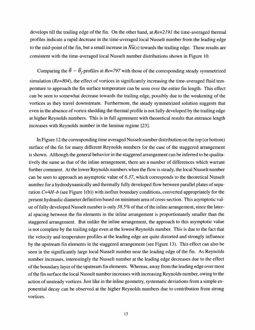
develops till the trailing edge of the fin. On the other hand, at Re=2191 the time-averaged thermal
profiles indicate a rapid decrease in the time-averaged local Nusselt number from the leading edge
to the mid-point of the fin, but a small increase in Nu(s) towards the trailing edge. These results are
consistent with the time-averaged local Nusselt number distributions shown in Figure 10.
Comparing the li - lif profiles at Re=797 with those of the corresponding steady symmetrized
simulation (Re=804), the effect of vortices in significantly increasing the time-averaged fluid tem
perature to approach the fin surface temperature can be seen over the entire fin length. This effect
can be seen to somewhat decrease towards the trailing edge, possibly due to the weakening of the
vortices as they travel downstream. Furthermore, the steady symmetrized solution suggests that
even in the absence of vortex shedding the thermal profile is not fully developed by the trailing edge
at higher Reynolds numbers. This is in full agreement with theoretical results that entrance length
increases with Reynolds number in the laminar regime [23].
In Figure 12 the corresponding time averaged Nusselt number distribution on the top (or bottom)
surface of the fin for many different Reynolds numbers for the case of the staggered arrangement
is shown. Although the general behavior in the staggered arrangement can be inferred to be qualita
tively the same as that of the inline arrangement, there are a number of differences which warrant
further comment. At the lower Reynolds numbers when the flow is steady, the local Nusselt number
can be seen to approach an asymptotic value of 6.37, which corresponds to the theoretical Nusselt
number for a hydrodynamically and thermally fully developed flow between parallel plates of sepa
ration C=4H-b (see Figure 1 (b)) with isoflux boundary conditions, converted appropriately for the
present hydraulic diameter definition based on minimum area of cross-section. This asymptotic val
ue of fully developed Nusselt number is only 38.5% of that of the inline arrangement, since the later
al spacing between the fin elements in the inline arrangement is proportionately smaller than the
staggered arrangement. But unlike the inline arrangement, the approach to this asymptotic value
is not complete by the trailing edge even at the lowest Reynolds number. This is due to the fact that
the velocity and temperature profiles at the leading edge are quite distorted and strongly influence
by the upstream fin elements in the staggered arrangement (see Figure 13). This effect can also be
seen in the significantly large local Nusselt number near the leading edge of the fin. As Reynolds
number increases, interestingly the Nusselt number at the leading edge decreases due to the effect
of the boundary layer of the upstream fin elements. Whereas, away from the leading edge over most
of the fin surface the local Nusselt number increases with increasing Reynolds number, owing to the
action of unsteady vortices. Just like in the inline geometry, systematic deviations from a simple ex
ponential decay can be observed at the higher Reynolds numbers due to contribution from strong
vortices.
13
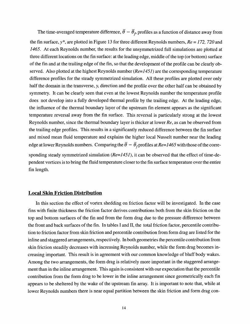
The time-averaged temperature difference, (j - (jf' profiles as a function of distance away from
the fin surface, y*, are plotted in Figure 13 for three different Reynolds numbers, Re = 172, 720 and
1465. At each Reynolds number, the results for the unsymmetrized full simulations are plotted at
three different locations on the fin surface: at the leading edge, middle of the top (or bottom) surface
of the fin and at the trailing edge of the fin, so that the development of the profile can be clearly ob
served. Also plotted at the highest Reynolds number (Re=1451) are the corresponding temperature
difference profiles for the steady symmetrized simulation. All these profiles are plotted over only
half the domain in the transverse, y, direction and the profile over the other half can be obtained by
symmetry. It can be clearly seen that even at the lowest Reynolds number the temperature profile
does not develop into a fully developed thermal profile by the trailing edge. At the leading edge,
the influence of the thermal boundary layer of the upstream fin element appears as the significant
temperature reversal away from the fin surface. This reversal is particularly strong at the lowest
Reynolds number, since the thermal boundary layer is thicker at lower Re, as can be observed from
the trailing edge profiles. This results in a significantly reduced difference between the fin surface
and mixed mean fluid temperature and explains the higher local Nusselt number near the leading
edge at lower Reynolds numbers. Comparing the (j - 8!profiles at Re=1465 with those of the corre-
sponding steady symmetrized simulation (Re=1451), it can be observed that the effect oftime-de
pendent vortices is to bring the fluid temperature closer to the fin surface temperature over the entire
fin length.
Local Skin Friction Distribution
In this section the effect of vortex shedding on friction factor will be investigated. In the case
fins with finite thickness the friction factor derives contributions both from the skin friction on the
top and bottom surfaces of the fin and from the form drag due to the pressure difference between
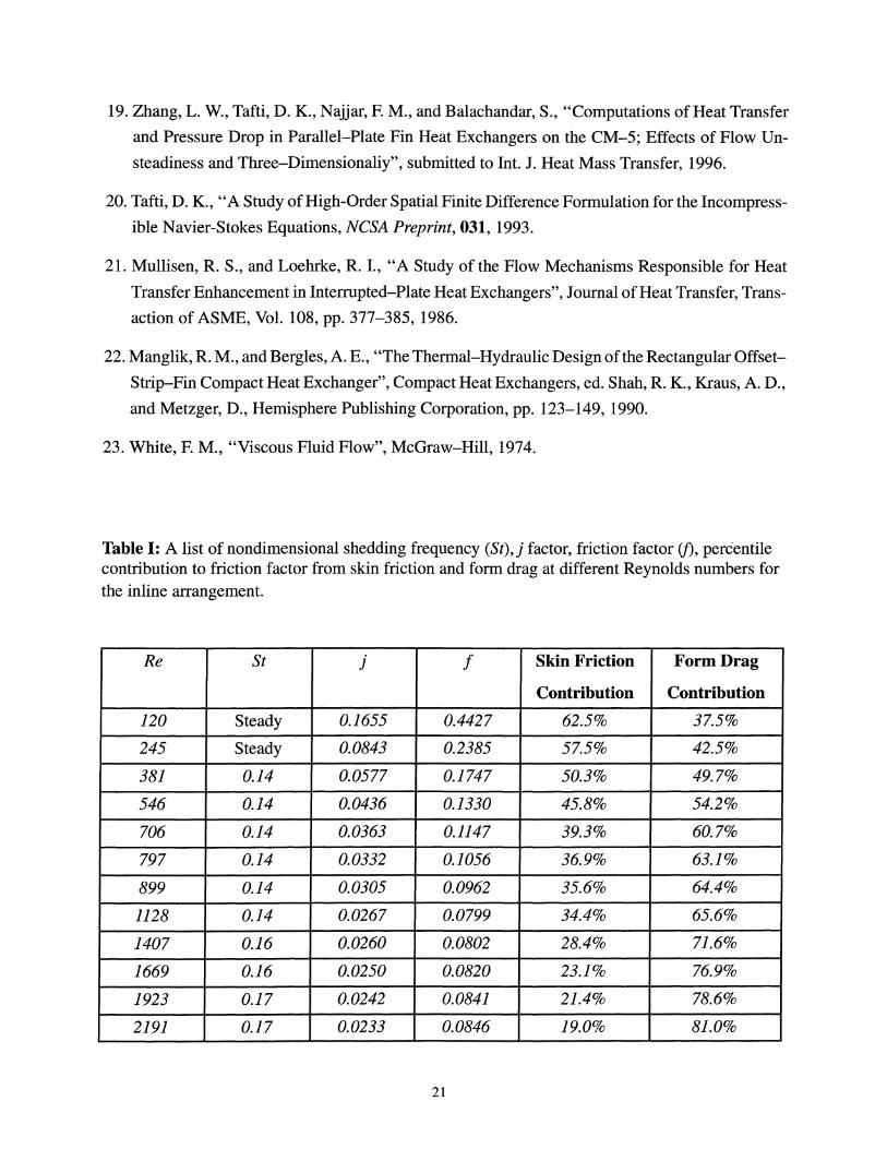
the front and back surfaces of the fin. In tables I and II, the total friction factor, percentile contribu
tion to friction factor from skin friction and percentile contribution from form drag are listed for the
inline and staggered arrangements, respectively. In both geometries the percentile contribution from
skin friction steadily decreases with increasing Reynolds number, while the form drag becomes in
creasing important. This result is in agreement with our common knowledge of bluff body wakes.
Among the two arrangements, the form drag is relatively more important in the staggered arrange
ment than in the inline arrangement. This again is consistent with our expectation that the percentile
contribution from the form drag to be lower in the inline arrangement since geometrically each fin
appears to be sheltered by the wake of the upstream fin array. It is important to note that, while at
lower Reynolds numbers there is near equal partition between the skin friction and form drag con-
14

tributions, at higher Reynolds number the form drag contribution is factor four or more greater than
the skin friction contribution.
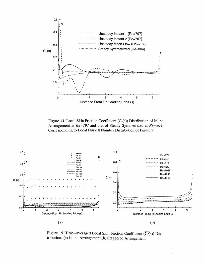
Figure 14 investigates the effect of the vortices that roll on the top and bottom surfaces of the
fin on local skin friction factor. Here local skin friction factor is defined as, Cf = ~ [~u] 2 D hVZ' Y wall ()
consistent with the overall friction factor defined in Eqn 9, which includes contribution from form
drag as well. The local skin friction factor on the top surface of the fin at Re=797 for the inline ar
rangement is plotted in Figure 14 at two different time instances shown in Figure 8. The correspond
ing local Nusselt number were presented earlier in Figure 9. It can be clearly seen by comparing
the q distribution with the vortex seen near the leading edge in Figure 8(b), that the effect of the
vortex for the most part is to decrease the local skin friction. In fact, due to the local reversed flow
induced by the vortex a negative skin friction, corresponding to a negative drag force, can be seen.
The weaker local maximum and minimum around s=0.8 and s=OA suggest the presence of smaller
counter rotating eddies (which are not large enough to be fully visible in Figure 8(b)) at the heel of
the larger clockwise rotating vortex. Downstream of the vortex, the skin friction factor quickly be
comes positive and approaches a near constant value of about 0.8. The effect of the vortices can also
be seen as the local minima at s=3.1 in the local skin friction factor distribution at the earlier time
corresponding to Figure 8(a), but the drop in qis not as dramatic due to the rapid decay of the vor
tices as they travel downstream.
Also plotted in this figure are the time-averaged local skin friction factor, Cis), for the unsteady
simulation and the local skin friction factor obtained from the corresponding steady symmetrized
simulation at Re=804. A comparison of the instantaneous distributions with the time averages dis
tribution clearly illustrates the strong effect of the vortices in decreasing local q by as much as 64%
near the leading edge. Of course, this effect significantly weakens downstream of the leading edge.
The significant decrease in the local skin friction factor obtained in the time-dependent simulation
over the corresponding steady state simulations can be attributed to the presence of vortices. Thus
the effect ofthe vortex on skin friction can be seen to be just the opposite of its effect on local Nusselt
number. Although the above results are for the inline arrangement, an investigation of the staggered
arrangement shows similar strong local reduction in the skin friction factor due to the vortices.
Figure 15(a) shows the time-dependent local skin friction for all the Reynolds numbers of the
inline arrangement. At the lowest Reynolds number of 120, the skin friction factor can be seen to
decay to an asymptotic value of about 0.505. This asymptotic value is in full agreement with the
theoretical friction factor of 60.63/Re corresponding to a fully developed parabolic flow between
parallel plates of separation C=2H-b, converted appropriately for the present hydraulic diameter
15
definition. Thus it can be seen that the boundary layer grows very rapidly to the fully developed
profile. At slightly higher Reynolds numbers, the effect of the finite fin thickness can seen as the
undershoot in the approach to the asymptotic value very close to the leading edge. Furthermore, the
approach to the asymptotic value appears very rapid and not strongly dependent on the Reynolds
number. This appears to be in contradiction to the theoretical prediction that the entrance length for
the development of the hydrodynamic boundary layer in a channel increases linearly with Re [23].
But it will soon be noted that the velocity profile even at the leading edge is close a parabolic profile
and significantly different from a plug flow assumed in the theory. The rapid increase in the friction
factor close to the trailing edge is due to the sudden expansion of the flow downstream of the trailing
edge.
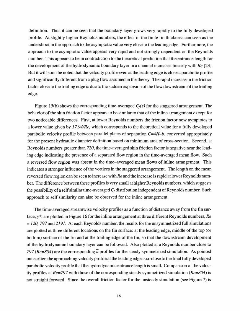
Figure 15 (b) shows the corresponding time-averaged Cfi s) for the staggered arrangement. The
behavior of the skin friction factor appears to be similar to that of the inline arrangement except for
two noticeable differences. First, at lower Reynolds numbers the friction factor now aymptotes to
a lower value given by 17.94IRe, which corresponds to the theoretical value for a fully developed
parabolic velocity profile between parallel plates of separation C=4H-b, converted appropriately
for the present hydraulic diameter definition based on minimum area of cross-section. Second, at
Reynolds numbers greater than 720, the time-averaged skin friction factor is negative near the lead
ing edge indicating the presence of a separated flow region in the time-averaged mean flow. Such
a reversed flow region was absent in the time-averaged mean flows of inline arrangement. This
indicates a stronger influence of the vortices in the staggered arrangement. The length on the mean
reversed flow region can be seen to increase with Re and the increase is rapid at lower Reynolds num
ber. The difference between these profiles is very small at higher Reynolds numbers, which suggests
the possibility of a self similar time-averaged qdistribution independent of Reynolds number. Such
approach to self similarity can also be observed for the inline arrangement.
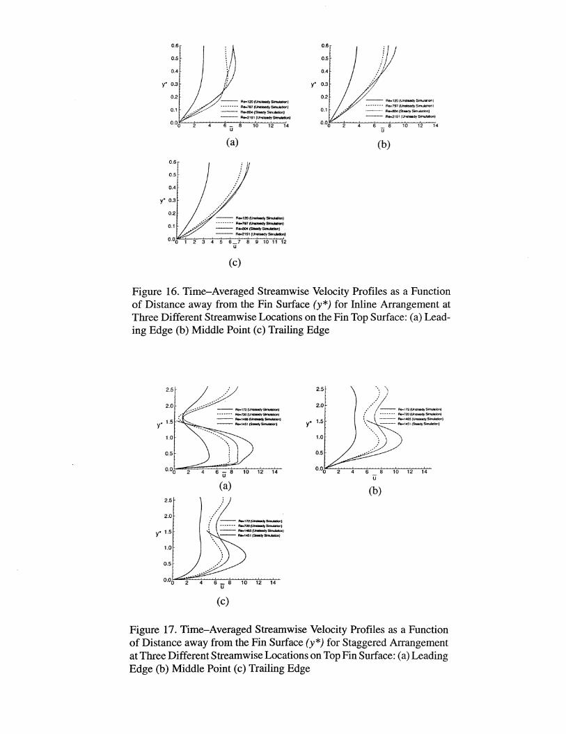
The time-averaged streamwise velocity profiles as a function of distance away from the fin sur
face, y*, are plotted in Figure 16 for the inline arrangement at three different Reynolds numbers, Re
= 120, 797 and 2191. At each Reynolds number, the results for the unsymmetrized full simulations
are plotted at three different locations on the fin surface: at the leading edge, middle of the top (or
bottom) surface of the fin and at the trailing edge of the fin, so that the downstream development
of the hydrodynamic boundary layer can be followed. Also plotted at a Reynolds number close to
797 (Re=804) are the corresponding "it profiles for the steady symmetrized simulation. As pointed
out earlier, the approaching velocity profile at the leading edge is so close to the final fully developed
parabolic velocity profile that the hydrodynamic entrance length is small. Comparison of the veloc
ity profiles at Re=797 with those of the corresponding steady symmetrized simulation (Re=804) is
not straight forward. Since the overall friction factor for the unsteady simulation (see Figure 7) is
16
larger, the corresponding time-averaged flow rate is 8.5% smaller than that of the steady symme
trized flow (note that in the present simulations the nondimensional pressure drop is held fixed equal
to unity in all the simulations). Thus part ofthe decreased local skin friction factor in the unsymme
trized simulation over the steady symmetrized simulation observed in Figure 14 is due to this de
creased time-averaged flow rate. This difference in flow rate is sufficient to account for the differ
ence at the mid-point of the fin and further downstream. Whereas, the larger difference close to the
leading edge is clearly due to the action of the vortices. While the unsteady flow phenomena at high
er Reynolds numbers is thus seen to decrease the skin friction contribution, its effect on form drag
is just the opposite. The form drag increases with flow oscillation and more than compensates for
the decrease in skin friction and thereby the overall friction factor is increased over the steady sym
metrized simulation.
Finally, the time-averaged streamwise velocity profiles as a function of distance away from the
fin surface, y*, are plotted in Figure 17 for the staggered arrangement at three different Reynolds
numbers: Re = 172, 720 and 1465. At each Reynolds number, the results for the un symmetrized full
simulations are plotted at three different locations on the fin surface: at the leading edge, middle of
the top surface of the fin and at the trailing edge of the fin. Also plotted are the corresponding stream
wise velocity profiles for the steady symmetrized simulation at Re=1451. All these profiles are
plotted over only half the domain in the transverse, y, direction. At the leading edge, the boundary
layer of the upstream fin element appears to strongly influence the velocity profile. A sharp decrease
in the streamwise velocity at y*=1.625 (mid way between the adjacent fin elements) accounts for
the significant departure from a parabolic profile. This decrease in the local velocity near the center
line somewhat increases the maximum velocity in order to conserve flow rate and furthermore the
location of the maximum velocity moves closer to the fin surface (y*~O.4). This results in a signifi
cantly increased velocity gradient at the fin surface and explains the higher local skin friction coeffi
cient near the leading edge. It can be clearly seen that even at the lowest Reynolds number the veloc
ity profile does not develop into a fully developed parabolic profile by the trailing edge. Comparing
the velocity profiles at Re=1465 with those of the corresponding steady symmetrized simulation
(Re=1451), it can be observed that the due to the increased overall friction factor the unsteady simu
lations result in a 15% smaller time-averaged flow rate than the steady symmetrized simulations.
The lower flow rate contributes to a lower skin friction coefficient in case of the unsteady simula
tions, and more importantly the effect of the vortices in the unsteady regime is to further decrease
the skin friction contribution. But, as seen in the inline arrangement, the effect of time-dependent
flow oscillation is to significantly increase the form drag and more than compensate for the decrease
in the skin friction contribution.
17

CONCLUSION
Here we have employed direct numerical simulations to explore the fluid flow and heat transfer
in parallel-plate heat exchangers in the time-dependent flow regime and this approach has proven
to be a very powerful tool in understanding the associated rich physics. The effect of vortex shedding
and and associated flow unsteadiness have been captured by solving the unsteady Navier-Stokes and
energy equations in two-dimensions. The flow field is assumed to be periodic along the streamwise
and transverse directions in order to simulate flow over a large array of identical fin elements. The
constant heat flux boundary condition employed in the present simulation allows for periodic
boundary condition to be applied for a modified temperature field. Both inline and staggered ar
rangement of fins are considered and results obtained from these simulations are compared with
those obtained from continuous parallel plates and the steady simulations of Sparrow & Liu [1] on
inline and staggered flat fins of infinitesimal thickness.
The inline and staggered arrangements are seen to increase heat transfer and friction factor over
a corresponding continuous parallel plate geometry (which maintains the same heat transfer surface
area) in significantly different ways. In the case of inline arrangement the lateral gap between adja
cent fins (C - see Figure la) available for through flow is more than halved. Thereby the velocity
and temperature gradients are increased resulting in significant increase in the j andJfactors. But
the velocity and temperature profiles approaching any fin element is not too far disturbed from the
fully developed profile that the real boundary layer restart mechanism is not very strong in this case.
In the case of staggered arrangement, the lateral gap between adjacent fin elements decreases only
slightly due to the finite thickness of the fin. On the other hand, owing to the staggered arrangement
the velocity and temperature profiles approaching any fin element are significantly distorted away
from the fully developed profile. The resulting increased velocity and thermal gradients at the fin
surface contribute to increasedj andJfactors.
Irrespective of the fin arrangement the flow is observed to follow a sequence of transitions. At
very low Reynolds numbers the flow is steady and above a critical Reynolds number flow becomes
unsteady with a single dominant frequency. At even higher Reynolds numbers an additional lower
frequency is generated and with subsequent increase in Re the flow becomes chaotic. In the inline
arrangement these transitions are observed at a higher Reynolds number than in the staggered ar
rangement. But in both arrangements the unsteady regime is marked by vortices that are generated
at the leading edges of the fin element, which travel down on the top and bottom surfaces of the fin
element. These vortices playa key role in significantly enhancing the local heat transfer by bringing
cold fluid towards the fin surface. On the other hand, the reversed flow generated by the vortices
near the fin surface is responsible for an overall reduction in skin friction on the fin surface.
18
The overall friction factor receives contribution from the form drag as well due to the wake be
hind the trailing end of the fin element. It is observed that the flow unsteadiness manifests itself in
the wake as waviness induced by vortex shedding and this significantly increases the form drag con
tribution. Since the form drag increases more than the decrease in skin friction, the overall drag also
increases due to time-dependent flow motion. This raises an interesting possibility that if vortices
that roll on the side surfaces of the fin be enhanced but the waviness in the wake be suppressed, en
hanced heat transfer may be achieved without pumping power penalty. It must be pointed out that
the vortex shedding on the front leading edges and flow waviness in the wake are intimately related,
with each influencing the other. But this is a line of thought that is worth pursuing in order to improve
the overall performance of the heat exchanger.
ACKNOWLEDGEMENT
This research was performed under a grant from the Air Conditioning and Refrigeration
Center at University of Illinois at Urbana-Champaign. The computation time was provided on a
massively parallel supercomputer(CM5) at National Center for Supercomputing Applications at
University of Illinois at Urbana-Champaign. The authors would like to acknowledge Professor A.
M. Jacobi and Graduate Research Assistant N. C. Dejong at the University of Illinois at Urbana
Champaign for many insightful discussions, comments and suggestions.
REFERENCES
1. Sparrow, E. M., and Liu, C. H., "Heat Transfer, Pressure-Drop and Performance Relationships
for Inline, Staggered, and Continuous Plate Heat Exchangers", Int. J. Heat Mass Transfer, Vol.
22, 1979, pp. 1613-1624.
2. Patankar, S. v., Liu, C. H., and Sparrow, E. M., "Fully Developed Flow and Heat Transfer in
Ducts Having Streamwise-Periodic Variations of Cross-Sectional Area", Journal of Heat Trans
fer, Transaction of ASME., Vol. 99, 1977, pp. 180-186.
3. Sparrow, E. M., Baliga, B. R., and Patankar, S. v., "Heat Transfer and Fluid Flow Analysis of
interrupted-Wall Channels, with Applications to Heat Exchangers", Journal of Heat Transfer,
Transaction of ASME, Vol. 99, 1977, pp. 4-11.
4. Cur, N., and Sparrow, E. M., "Experiments on Heat Transfer and Pressure Drop for a Pair of Coli
near, Interrupted Plates Aligned with the Flow", Int. J. of Heat Mass Transfer, 1978, Vol. 21, pp.
1069-1080.
19
5. Sparrow, E. M., and Hajiloo, A, "Measurements of Heat Transfer and Pressure Drop for an Array
of Staggered Plates Aligned Parallel to an Air Flow", Journal of Heat Transfer, Transaction of
ASME, Vol. 102, 1980, pp. 426-432.
6. Patankar, S. v., and Prakash, c., "An Analysis of the Effect of Plate Thickness on Laminar Flow
and Heat Transfer in Interrupted-Plate Passages", Int. J. of Heat Mass Transfer, Vol., 24,1981,
pp.51-58.
7. Mullisen, R S., and Loehrke, R I., "A Study of the Flow Mechanics Responsible for Heat Trans
fer Enhancement in Interrupted-Plate Heat Exchangers", Journal of Heat Transfer, Transaction
of ASME, Vol. 108, 1986, pp. 377-385.
8. Ghaddar, N. K, Karniadakis, G. E., and Patera, A T, "A Conservative Isoparametric Spectral
Element Method for Forced Convection; Application to Fully Developed Flow in Periodic Ge
ometries", Numerical Heat Transfer, Vol. 9, 1986, pp. 277-300.
9. Amon, C. H. and Mikic, B. B., "Spectral Element Simulations of Unsteady Forced Convective
Heat Transfer: Application to Compact Heat Exchanger Geometries", Numerical Heat Transfer,
Part A, Vol. 19, 1991, pp. 1-19.
1 0. Jacobi, AM. and Shah, RK, Heat transfer surface enhancements through the use oflongitudinal
vortices: A review of recent progress, submitted to Exp. Thermal Fluid Sci., 1995.
11. Fiebig, M., Vortex generators for compact heat exchangers, 1. Enhanced Heat Transfer, (in
press), 1995.
12. Mittal, R, and Balachandar, S., "Effect of Three-Dimensionality on the Lift and Drag ofCircu
lar and Elliptic Cylinders", (in press) Physics of Fluids, 7, 1995.
13. Williamson, C.H.K, and Roshko, A, "Measurements of Base Pressure in the Wake of a Cylin
der at Low Reynolds Numbers", Z. Flugwiss. Weltraumforch, 14,36, 1990.
14. Sychev, v.v., "Asymptotic theory of separated flows", Mekh. Zh. Gaza, 2, 20, 1982.
15. Suzuki, K, Hirai, E., Miyaki, T, and Sato, T, "Numerical and Experimental Studies on a Two
Dimensional Model of an Offset Strip-Fin Type Compact Heat Exchanger Used at Low Re
ynolds Number", Int. J. Heat Mass Transfer, Vol. 28, pp. 823-836, 1985.
16. Joshi, H. M., and Webb, R L., "Heat Transfer and Friction in the Offset Strip-Fin Heat Exchang
er", Int. J. Heat Mass Transfer, Vol. 30, pp. 69-84, 1987.
17. Amon, C. H., "Heat Transfer Enhancement and Three-Dimensional Transitional Flows by a
Spectral Element-Fourier Method", Ph.D. Thesis, MIT, 1988.
18. Harlow, F. H., and Welch, J. E., "Numerical Calculation of Time-Dependent Viscous Incom
pressible Flow of Fluid with Free Surface, Phys. Fluids, Vol. 8, No. 12, pp. 2181-2189, 1965.
20
19. Zhang, L. W., Tafti, D. K, Najjar, F. M., and Balachandar, S., "Computations of Heat Transfer
and Pressure Drop in Parallel-Plate Fin Heat Exchangers on the CM-5; Effects of Flow Un
steadiness and Three-Dimensionaliy", submitted to Int. J. Heat Mass Transfer, 1996.
20. Tafii, D. K, "A Study of High-Order Spatial Finite Difference Formulation for the Incompress
ible Navier-Stokes Equations, NCSA Preprint, 031, 1993.
21. Mullisen, R. S., and Loehrke, R. I., "A Study of the Flow Mechanisms Responsible for Heat
Transfer Enhancement in Interrupted-Plate Heat Exchangers", Journal of Heat Transfer, Trans
action of ASME, Vol. 108, pp. 377-385, 1986.
22. Manglik, R. M., and Bergles, A. E., "The Thermal-Hydraulic Design of the Rectangular Offset
Strip-Fin Compact Heat Exchanger", Compact Heat Exchangers, ed. Shah, R. K, Kraus, A. D.,
and Metzger, D., Hemisphere Publishing Corporation, pp. 123-149, 1990.
23. White, F. M., "Viscous Fluid Flow", McGraw-Hill, 1974.
Table I: A list of nondimensional shedding frequency (St),j factor, friction factor (j), percentile contribution to friction factor from skin friction and form drag at different Reynolds numbers for the inline arrangement.
Re St j f Skin Friction Form Drag
Contribution Contribution
120 Steady 0.1655 0.4427 62.5% 37.5%
245 Steady 0.0843 0.2385 57.5% 42.5%
381 0.14 0.0577 0.1747 50.3% 49.7%
546 0.14 0.0436 0.1330 45.8% 54.2%
706 0.14 0.0363 0.1147 39.3% 60.7%
797 0.14 0.0332 0.1056 36.9% 63.1%
899 0.14 0.0305 0.0962 35.6% 64.4%
1128 0.14 0.0267 0.0799 34.4% 65.6%
1407 0.16 0.0260 0.0802 28.4% 71.6%
1669 0.16 0.0250 0.0820 23.1% 76.9%
1923 0.17 0.0242 0.0841 21.4% 78.6%
2191 0.17 0.0233 0.0846 19.0% 81.0%
21
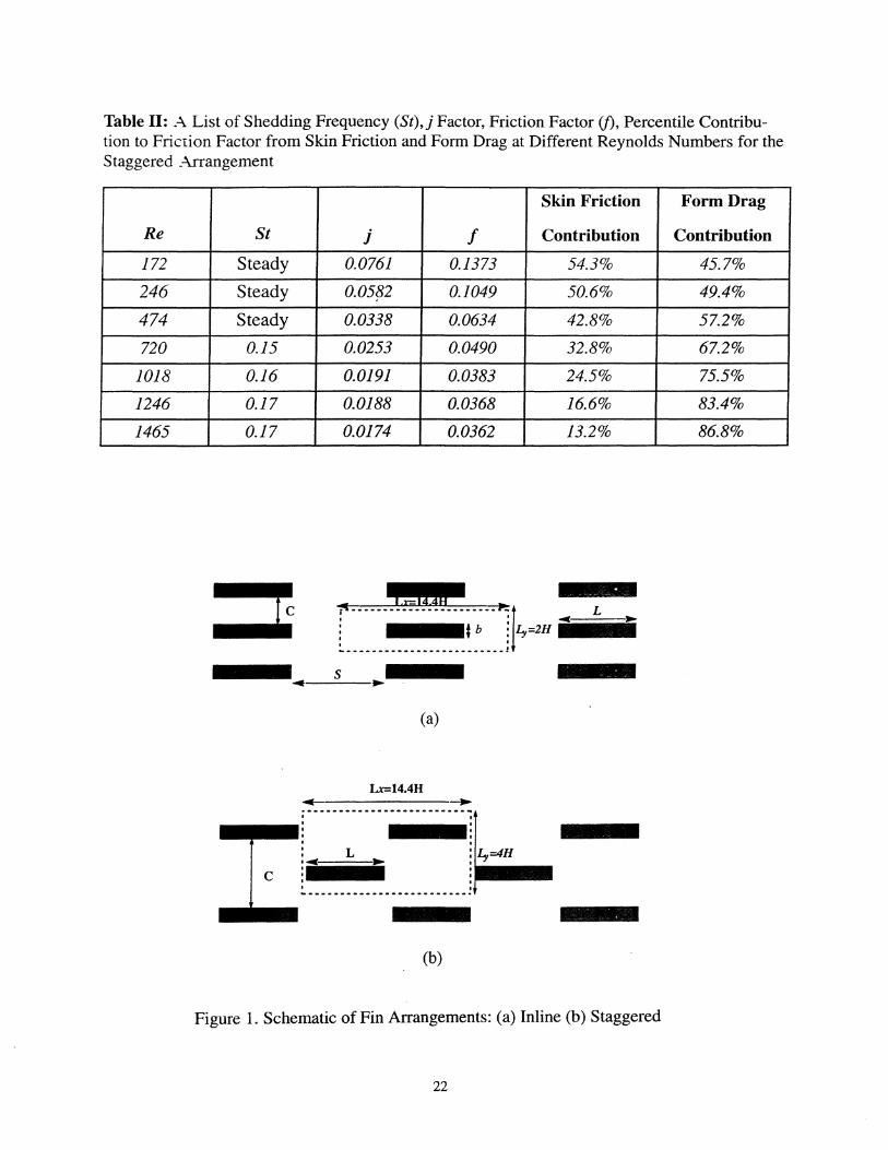
Table II: A. List of Shedding Frequency (St),j Factor, Friction Factor (j), Percentile Contribution to Friction Factor from Skin Friction and Form Drag at Different Reynolds Numbers for the Staggered _-\rrangement
Skin Friction Form Drag
Re St j f Contribution Contribution
172 Steady 0.0761 0.1373 54.3% 45.7%
246 Steady 0.0582 0.1049 50.6% 49.4%
474 Steady 0.0338 0.0634 42.8% 57.2%
720 0.15 0.0253 0.0490 32.8% 67.2%
1018 0.16 0.0191 0.0383 24.5% 75.5%
1246 0.17 0.0188 0.0368 16.6% 83.4%
1465 0.17 0.0174 0.0362 13.2% 86.8%
• __ b=1l4d __ f'··-···············;·;··~ILy=211 ii4CiiiiLiiiiii~ , . ~ _________________________ 1
(a)
Lx=14.4H ..- -.. 1-·····::·················]1,=411 . . ~ ~ ,"" , . , . , , , , ~-------------------------.
c
• (b)
Figure 1. Schematic of Fin Arrangements: (a) Inline (b) Staggered
22
0.5
0.0
.(1.5
-1.0
<Nu(I»
15
14
13
12
-1.s~~~ 11
1030'=--------4*O------SO;f,;· -------;560 Nondimensional Time
1.5
1.0
0.5
0.0
.(1.5
-1.0
-1.5
(a)
15.83
15.82
15.81
15.80
<Nu(I» 15.79
15.78
15.n
15.76
15. 75 L--.1-:;,06;------,1'*07 ........ -T.\108;a--Ttl09\1>~11 in10~--:;1t;11r-.-....,1;t12,Nondimensional Tome
(b)
21.0
20.8
20.6
<Nu(,,> 20.4
20.2
20.0
19.8
19.6 L---:><----,;;,..--A'A--""""4'6--Ts--50--52" 40 42 44 46
Nondimensional Time
(c)
24.0
23.5
23.0
22.5
22.0 <Nu(I»
21.5
21.0
20.5
2O'Q35 lSO
(d)
Figure 2. Vector Plot of Velocity Field and Time Trace of Instantaneous Global Nusselt Number for
the Staggered Arrangement: (a) Re=246, the Flow is Steady (b) Re=720, the Flow Oscillates at a
Single Frequency with a Strouhal Number of 0.15 (c) Re=1245, the Strouhal Number of the Primary
Frequency is 0.17, a Secondary Low Frequency with a Strouhal Number of 0.036 can also be ob
served (d) Re=1465, the Flow is Chaotic
155

0.5
0.0
-0.5
* 0.5 , ,
, 0.0 , , , ,
2: 2}
-0.5 ,
0.30
0.25
0.20
0.15
0.09
0.04 .(l.01
.(l.06
Figure 3. Contour Plot of Perturbation Temperature (8) for the Staggered Arrangement Corresponding to Figure 2(d) (Re=1465)
2~ : ' , , , ,
8 0.30
7 0.25
,/ -\: 2"'-\ _---' ~.I?:' \, ~" -' ' ',-' ",
, 2,',',' 2 , " f
I i 6 0.20 , , , , 2
5 0.15
4 0.09
3 0.04
2 ·0.01
1 ·0.06
f ~ \ ~,I I
I " \ /'. f I \ \ . I I I . \ \?~ \ I 2 \ I ~~ \ I , \ I ,I \
T I \ I I I \
i 2' \2/: 4 ? ,'---- ~~?7(: ": :2 ,', " ~ I ..... ------./ \--~ /' I I ' 2' , ... , ........ ,... 3 I 2 f I
.. - ... \ : '2.. ' I I,: ~
'2, ,/ I' !: 2 4 6 8 10 14
Figure 4. Instantaneous Flow and Temperature Patterns for Inline Arrangement at Re= 1407: (a) Vector Plot of Velocity Field (b) Contour Plot of Perturbation Temperature (8)
(a)
(b)

10-2
10
... ~. MuItisen& t..oehI1<e
-- Simulalion· P_& P_ ••••••• ~lon·Joshi&W_
-- Correlation - Manglik & lle<gIes
--v-- Staggered Unsteady Simulation
10 Re
(a)
10·
...
10~
... ExperimenIs - MuIIIsen & t..oehI1<e -- Simulation - PatanQr & Ptakash • ••••• • Corretauon - Joshi & W_ --- Correlalion - Manglik & Bergles --":I-- Staggered Unsteady Simulation
... -... ... ...
10 Re
(b)
...
Figure 5. A Comparison of Current results for the Staggered arrangement with those available in
Literature: (a)j factor vs Reynolds Number (b) friction factor if) vs Reynolds Number
10
-- Fully Developed B. L. - - - - - - - Restarted B. L. (Sparrow & Liu)
--v-- Staggered Unsteady Simulation _._-_ .... _.- Staggered Steady Simulation
f
10 Re
(a)
10~
10
-- Fully Developed B. L. ••••••• Restarted B. L. (Sparrow & Uu}
--":I-- Staggered Unsteady Simutation •. _._-- Staggered Sleady Simulation
---
Re 10
(b)
Figure 6. A Comparison ofIndividual Enhancement Mechanisms and the Effect on Friction Factor in Staggered Arrangement: (a) j vs Reynolds Number (b)fvs Reynolds Number
-- Fully Developed B. L. ••••••• Restart B.L. (Sparrow & Liu)
--v-- Imine Unsteady Simulation --.---- Inline Steady Simulation
10 Re
(a)
10·
10~
.........
-- Fully Developed B. L. ••••••• Restarted B. L.l§panow & Uu)
--v-- Inline Unsleady Simutation • -_._._-- Infine Steady Simutation
10 Re
(b)
Figure 7. A Comparison of Individual Enhancement Mechanisms and the Effect on Friction Factor in Inline Arrangement: (a) j vs Reynolds Number (b)fvs Reynolds Number
0.5
0.0 (a)
-0.5
0.5
0.0 (b)
-0.5
Figure 8. Vector Plot of Instantaneous Velocity Fields for the Inline Arrangement at Re=797. (a)
Instant 1 (b) Instant 2, Approximately 0.5 Nondimensional Time Units After Instant 1.
Nu(s)
60
A 50
40
20
Unsteady Instant 1 (Re=797)
- - - - - - - - Unsteady Instant 2 (Re=797) _._._._._._._.- Unsteady Mean Flow (Re=797)
..................... Steady Symmetrized (Re=804)
s
DA
~ " " " ,A , ,
Figure 9. A Comparison of Local Nusselt Number Distribution for the Inline Arrangement at
Re=797 at the Two Instances in Time Shown in Figure 8. Also Shown are the Time Averaged Local
Nusselt Number Distribution and the Corresponding Result for the Steady Symmetrized Simulation
at Re=804
80
40
30
20
-- Re=120 ------ Re--245 -.-.-.-.-.- Re--381 ••••......•.••• Re--546
----- Re=706 _ .. - .. - .. _ .. - Re=797
-II- Re=899
-- Re=1128 ~ Re=1407
~ Re=1669
Re=1923 I>
I> Re=2191
2 3 4 5 6
Distance From Fin Leading Edge (5)
Figure 10. Time-Averaged Nusselt Number Distribution on Top Fin Surface of the Inline Arrangement
0.6
0.5
0.4
y' 0.3
0.2 -- ~120(unsteadysmulalion) ....... _797(~_"",'
0.1 -- _(51eady_"",) -- ~191 (UnsteadySimufalion)
0.0 .0.40
0.6
0.5
0.4
y' 0.3
0.2
: t : .
(a)
\, ...... . -- =-t20(Unoteady_)
---- -- - =..797 (UnSteady SImulation) 0.1 ._. __ (Steady_""')
-- -.,., (UnoteadySlmWotion)
.. ! •
\ : 1 :
\j \\ \~
\. ~~
-0.10
0.0 '---"-;;-o1-4:--~"""0~3"'""""'~"""-o~2"'""""'~"""-0~.1""""'~~ . - . 9- 9 . I
(c)
0.6
\;... 1\,11 ";:" '~~.
-- Ae.=120(Uns1eadySimulation) ..
0.5
0.4
y. 0.3
0.2
- - - - - - - Reo. 797 (l.InSI:eady Simulalion) 0.1 - ... ---- Re=804 (Steady Simulat"""
-- Ae=2191 (UnstNdy Simul'alionl
0.0 ~"-;;.0!-:.4"--~-::.01-,:.3""_~_---;;-o1-,:.2"----::.0;-'.1-~~ a -af
(b)
Figure 11. Time-Averaged Temperature Difference as a Function of Distance away from the Fin
Surface for the Inline Arrangement at Three Different Streamwise Locations: (a) Near the Leading
Edge (b) Middle Point along the Top Surface of the Fin (c) Near the Trailing Edge

80
70
60 .
Nu(s) 50
40
20
10
o
--- Re=172 Re=246 Re=474 Re=720
-----. Re=1018 _.--.. _ .. _ ... Re=1246
Re=1465
2 3 4 5
Distance From Fin Leading Edge (5)
, 1 ,
6
Figure 12. Time-Averaged Local Nusselt Number (Nu(s)) Distribution on Top Fin Surface of the Staggered Arrangement
2.5
2.0
1.0
0.5
0.0 .0.6 .0.4 0.4
2.5
I 2.0 1-- _172(unsteadySimulatlOn) I •..•••. _720 (Un.-ySimulatlOn)
1 __ ·- _1_ (Unsteady SImulatIOn)
-- Re.I451 (SIaady SImulatIOn) y* 1.5
1.0
0.5
0.0 -0.6 .0.4 0.2 0.4
(c)
2.5
2.0
y* 1.5
1.0
0.5
0.0 .0.6 .0.4
,
) : 1-- Ra-172(UnstaedySimutaUon) , !.............. Rea720 (Unsteady SfnlJlatlon)
j-_._. _1465(UnsteadySimulatlOn)
j-- Ae=1451 (SteedySimuladon)
( \
0.2 0.4
(b)
Figure 13. Time-Averaged Temperature Difference as a Function of Distance away from the Fin
Surface for the Staggered Arrangement at Three Different Streamwise Locations: (a) Near the Lead
ing Edge (b) Middle Point along the Top Surface of the Fin (c) Near the Trailing Edge
1.0
0.8 A
0.6
C,(S) . ... ... ...
0.4
0.2
0.5
0.4
\ \ I
A
0.3 I
0.2
o
\ \ ,
Unsteady Instant 1 (Re=797)
Unsteady Instant 2 (Re=797)
Unsteady Mean Flow (Re=797)
Steady Symmetrized (Re=804)
234 5
Distance From Fin Leading Edge (s)
B
6
Figure 14. Local Skin Friction Coefficient (Cf{s» Distribution of Inline Arrangement at Re=797 and that of Steady Symmetri~ed at Re=804, Corresponding to Local Nusselt Number Distribution of Figure 9
_'20 Do Re-24S o Rea381
- - - - - _106 _._._._.- _791
·············_99 ---- Re-1128 _ .. _ .. _-- _,407 --_,669 - - ~ - - _,923 ~- Re=.2191
A ... ... ... ... ... ... ... • ...
B
C,(s)
1.0 Re=172
-------- Re=246 A 0.8 _._._._._._._.-
Re=474 ..................... Re=720 ------- Re=1018
0.6 _ .. _ .. _ .. _ .. _ .. _., Re=1246 Re=1465
0.4
I
B
0.2 I " ! 1 , .'
0.0 \'~; .. ~.;::;~:~.;;; .. ::::.:; .. ::::. .. ; .. :::;:::::.:; .. ::::.:; .. ~:;:;.;:; .. ; .. ~:; .. ;.;:::;~:;.;;~:~;<."
2 3 4 5 6 o 2 3 4
Distance From An Leading Edge (s) Distance From Fin Leading Edge (s)
(a) (b)
Figure 15. Time-Averaged Local Skin Friction Coefficient (Cf{s» Distribution: (a) Inline Arrangement (b) Staggered Arrangement
5 6
0.6
0.5
0.4
y' 0.3
0.2
0.6
0.5
0.4
y' 0.3
0.2
0.1
4 6 _ 8 10 12 14
..-
U
(a)
j J
/./ ' /'"
,,/o' ~
_,.- -- Re00120(Unst~SimuIallon) ,/ -------- Rez7D7(UnsI9lIdySimuIaUon)
.' -- Re=804(Steec1ySimulatlon)
-- Re=2191 (Unsteady SImulation)
(c)
0.6
0.5
0.4
y' 0.3
0.2
0.1
: I
.f/ : /
:::/
;/ ;/
// -- Re:<l20(UnsteadySlmuletion)
~ ~ -------- Ae=191 (Uns1eadySimulanon) ... ----..•.• - R~ ($1eedy Simulation)
• -- Re=2191 (Unsteady Simulation)
4 8 10 12 14 IT
(b)
Figure 16. Time-Averaged Streamwise Velocity Profiles as a Function of Distance away from the Fin Surface (y*) for Inline Arrangement at Three Different Streamwise Locations on the Fin Top Surface: (a) Leading Edge (b) Middle Point (c) Trailing Edge
2.5
2.0
y' 1.5
1.0
0.5
2.5
2.0
y' 1.5
1.0
0.5
.. "-"'-';~"72' __ "1
--.---- Re00720 (Unsleady SImulation)
-- "'485~SIrMation) --F\e-14!1(SleadySlmulatiolll
(a)
:' -- Ae-172(~SImuIatIonI : --.---- Ae-720(lkmMdySlmu/allon)
• -- .... ,~(UnMadySimulallonl
\"') -'''''''--1
--'-""''''''
(c)
" .~.
.)) 2.5
/ .... ;1-- Re.,lnCUrweadySimuiationl
( (.:~= ::;ucu:s::::, ..... -- Re001451 (SI8adVSlmulalIon)
2.0
y' 1.5
..... ::;) 1.0
0.5
6 8 10 12 14
(b)
Figure 17. Time-Averaged Streamwise Velocity Profiles as a Function of Distance away from the Fin Surface (y*) for Staggered Arrangement at Three Different Streamwise Locations on Top Fin Surface: (a) Leading Edge (b) Middle Point (c) Trailing Edge
Top Related