


Languages
Pages
Legal


HARDWARE ACCELERATION OFSIMILARITY QUERIES USING GRAPHIC
PROCESSOR UNITS
a thesis
submitted to the department of computer engineering
and the institute of engineering and science
of bilkent university
in partial fulfillment of the requirements
for the degree of
master of science
By
Atilla Genc.
January, 2010
I certify that I have read this thesis and that in my opinion it is fully adequate,
in scope and in quality, as a thesis for the degree of Master of Science.
Asst. Prof. Dr. Ibrahim Korpeoglu(Supervisor)
I certify that I have read this thesis and that in my opinion it is fully adequate,
in scope and in quality, as a thesis for the degree of Master of Science.
Dr. Cengiz C. elik(Co-Supervisor)
I certify that I have read this thesis and that in my opinion it is fully adequate,
in scope and in quality, as a thesis for the degree of Master of Science.
Asst.Prof. Ali Aydın Selcuk
ii

I certify that I have read this thesis and that in my opinion it is fully adequate,
in scope and in quality, as a thesis for the degree of Master of Science.
Asst.Prof. Ozcan Ozturk
I certify that I have read this thesis and that in my opinion it is fully adequate,
in scope and in quality, as a thesis for the degree of Master of Science.
Asst.Prof. Tansel Ozyer
Approved for the Institute of Engineering and Science:
Prof. Dr. Mehmet B. BarayDirector of the Institute
iii
ABSTRACT
HARDWARE ACCELERATION OF SIMILARITYQUERIES USING GRAPHIC PROCESSOR UNITS
Atilla Genc.M.S. in Computer Engineering
Supervisor: Asst. Prof. Dr. Ibrahim Korpeoglu
Co-Supervisor: Dr. Cengiz C. elik
January, 2010
A Graphic Processing Unit (GPU) is primarily designed for real-time render-
ing. In contrast to a Central Processing Unit (CPU) that have complex instruc-
tions and a limited number of pipelines, a GPU has simpler instructions and many
execution pipelines to process vector data in a massively parallel fashion. In ad-
dition to its regular tasks, GPU instruction set can be used for performing other
types of general-purpose computations as well. Several frameworks like Brook+,
ATI CAL, OpenCL, and Nvidia Cuda have been proposed to utilize computa-
tional power of the GPU in general computing. This has provided interest and
opportunities for accelerating different types of applications.
This thesis explores ways of taking advantage of the GPU in the field of metric
space-based similarity searching. The KVP index structure has a simple organi-
zation that lends itself to be easily processed in parallel, in contrast to tree-based
structures that requires frequent ”pointer chasing” operations. Several imple-
mentations using the general purpose GPU programming frameworks (Brook+,
ATI CAL and OpenCL) based on the ATI platform are provided. Experimental
results of these implementations show that the GPU versions presented in this
work are several times faster than the CPU versions.
Keywords: Similarity Search, General Purpose Computing on Graphic Processing
Units, GPGPU.
iv
OZET
GRAFIK ISLEMCI BIRIMLERI KULLANILARAKBENZERLIK SORGULARININ HIZLANDIRILMASI
Atilla Genc.Bilgisayar Muhendisligi, Yuksek Lisans
Tez Yoneticisi: Asst. Prof. Dr. Ibrahim Korpeoglu
Tez Yoneticisi: Dr. Cengiz C. elik
Ocak, 2010
Grafik Isleme Birimi (GPU) birincil olarak gercek zamanlı goruntu olusturmak
icin tasarlanmıstır. Karmasık komut kumesi ve sınırlı ardısık duzene sahip
merkezi islem biriminin aksine GPU daha basit bir komut kumesine ve vektor
verilerini kosut olarak calıstırabilecek cok sayıda yurutme ardısık duzenine sahip-
tir. Olagan gorevlerine ek olarak, GPU komut kumesi baska tip genel amaclı
hesaplamalar icin kullanılabilir. GPU’ların islem gucunu genel amaclı hesapla-
malarda degerlendirebilmek icin Brook+, ATI CAL, OpenCL ve Nvidia Cuda gibi
degisik programlama cerceve modelleri onerilmistir. Bu durum pek cok uygula-
manın hızlandırılması icin fırsat dogurmustur.
Bu calısmada metrik tabanlı benzerlik araması alanında grafik kartlarının
sagladıgı avantajların kullanılması incelenmektedir. Sıkca ”imlec takibi” gerek-
tiren agac temelli yapıların aksine, KVP yapısı basit organizasyonu nedeniyle
kolayca kosut olarak islenmeye uygundur. ATI platformunda degisik genel
amaclı GPU programlama cerceve modelleri kullanılarak (Brook+, ATI CAL
ve OpenCL) Brute Force Linear Scan ve KVP algoritmaları gerceklestirilmis,
yapılan calısma sunulmustur. Bu gerceklestirimlerin deneysel sonuları GPU uygu-
lamalarının CPU surumlerinden cok daha hızlı oldugunu gostermektedir.
Anahtar sozcukler : Benzerlik Araması, Grafik Isleme Unitelerinde Genel Amaclı
Hesaplama, GPGPU.
v

Acknowledgement
I would like to thank my supervisors, Asst. Prof. Dr. Ibrahim Korpeoglu and
Dr. Cengiz C. elik for their guidance throughout my study.
vi

Contents
1 Introduction 1
2 Similarity Search 3
2.1 Overview . . . . . . . . . . . . . . . . . . . . . . . . . . . . . . . . 3
2.2 Survey on Related Work . . . . . . . . . . . . . . . . . . . . . . . 9
2.2.1 Clustering-Based Methods . . . . . . . . . . . . . . . . . . 11
2.2.2 Local Pivot-Based Methods . . . . . . . . . . . . . . . . . 12
2.2.3 Vantage-Point Methods . . . . . . . . . . . . . . . . . . . . 14
2.3 KVP Algorithm . . . . . . . . . . . . . . . . . . . . . . . . . . . . 16
2.3.1 The KVP Structure . . . . . . . . . . . . . . . . . . . . . 16
2.3.2 Secondary Storage . . . . . . . . . . . . . . . . . . . . . . 18
2.3.3 Memory Usage . . . . . . . . . . . . . . . . . . . . . . . . 19
2.3.4 Comparison of KVP and Tree-Based Structures . . . . . . 20
3 General Purpose Computing On GPU 22
3.1 Overview Of Graphics Hardware . . . . . . . . . . . . . . . . . . . 24
vii

CONTENTS viii
3.1.1 Programmable hardware . . . . . . . . . . . . . . . . . . . 26
3.2 GPU Programming Model . . . . . . . . . . . . . . . . . . . . . . 27
3.2.1 GPU Program Flow . . . . . . . . . . . . . . . . . . . . . 29
3.2.2 GPU Programming Systems . . . . . . . . . . . . . . . . . 32
3.2.3 GPGPU languages and libraries . . . . . . . . . . . . . . . 33
3.2.4 Debugging tools . . . . . . . . . . . . . . . . . . . . . . . . 35
3.3 GPGPU Techniques . . . . . . . . . . . . . . . . . . . . . . . . . 37
3.3.1 Stream operations . . . . . . . . . . . . . . . . . . . . . . . 37
3.3.2 Data Structures . . . . . . . . . . . . . . . . . . . . . . . . 43
3.4 GPGPU applications . . . . . . . . . . . . . . . . . . . . . . . . . 45
4 Implementation of Algorithms 52
4.1 Brute Force Search Implementation on GPU . . . . . . . . . . . . 57
4.2 KVP Implementation GPU . . . . . . . . . . . . . . . . . . . . . 63
4.3 Filtering Results on GPU . . . . . . . . . . . . . . . . . . . . . . 69
5 Experiment Results 75
5.1 Comparison of implementations with Result Set Filtering on CPU 77
5.2 Performance Overhead of Data Transfers from GPU to CPU . . . 81
5.3 Comparison of implementations with Result Set Filtering on GPU 86
6 Conclusion 90

List of Figures
2.1 Visualization of distance bounds. Given distances d(q, p) and
d(p, o) upper and lower bounds on d(q, o) can be established us-
ing triangle inequality (a) d(q, o) ≥ |d(q, p)− d(p, o)| (b) d(q, 0) ≤d(q, p) + d(p, o) . . . . . . . . . . . . . . . . . . . . . . . . . . . . 6
2.2 Possible partitioning of a set of objects. (a)ball partitioning and
(b) generalized hyperplane partitioning. . . . . . . . . . . . . . . . 8
2.3 A sample database of 9 vectors in 2-dimensional space, and an ex-
ample of the KVP structure on this database that keeps 2 distance
values per database object. (a) The location of objects. Boxes rep-
resent objects that have been selected as pivots. (b) The distance
matrix between pivots and regular database objects. For each ob-
ject, the 2 most promising pivot distances are selected to be stored
in KVP (indicated by using gray background color). (c) The first
three object entries in the KVP. Each object entry keeps the id of
the object, and an array of pivot distances. . . . . . . . . . . . . . 18
2.4 Query performance of the KVP structure, for vectors uniformly
distributed in 20 dimensions. . . . . . . . . . . . . . . . . . . . . . 19
3.1 The modern graphics hardware pipeline. The vertex and fragment
processor stages are both programmable by the user. . . . . . . . 25
ix

LIST OF FIGURES x
4.1 Serialized representation of objects. . . . . . . . . . . . . . . . . . 58
4.2 Packed instruction execution. . . . . . . . . . . . . . . . . . . . . 61
4.3 Iteratively counting number of objects in result set. . . . . . . . . 72
5.1 Execution times in seconds for 1000 radius queries on 220 vectors,
with varying vector dimensions. Result set filtering performed on
CPU. . . . . . . . . . . . . . . . . . . . . . . . . . . . . . . . . . . 78
5.2 Relative speeds of implementations for test set 1, when result set
filtering is performed on CPU. . . . . . . . . . . . . . . . . . . . . 78
5.3 Execution times in seconds for 1000 radius queries on vectors with
16 dimensions and varying number of vectors. Result set filtering
performed on CPU. . . . . . . . . . . . . . . . . . . . . . . . . . . 80
5.4 Relative speeds of implementations for test set 2, when result set
filtering is performed on CPU. . . . . . . . . . . . . . . . . . . . . 80
5.5 Execution times in seconds for 1000 radius queries on object set
size of 220 vectors, with varying vector dimensions, no result set
fetching. . . . . . . . . . . . . . . . . . . . . . . . . . . . . . . . . 82
5.6 Relative speeds of implementations for test set 1, no result set
fetching. . . . . . . . . . . . . . . . . . . . . . . . . . . . . . . . . 82
5.7 Execution times in seconds for 1000 radius queries on vectors with
16 dimensions and varying number of vectors, no result set fetching.. 85
5.8 Relative speeds of implementations for test set 2, no result set
fetching. . . . . . . . . . . . . . . . . . . . . . . . . . . . . . . . . 85
5.9 Execution times for 1000 radius queries on object set size of 220
vectors, with varying vector dimensions, GPU result set filtering. . 87
LIST OF FIGURES xi
5.10 Relative speeds of implementations for test set 1, GPU result set
filtering. . . . . . . . . . . . . . . . . . . . . . . . . . . . . . . . . 87
5.11 Execution times for 1000 radius queries on vectors with 16 dimen-
sions and varying number of vectors, GPU result set filtering. . . 88
5.12 Relative speeds of implementations for test set 2, GPU result set
filtering. . . . . . . . . . . . . . . . . . . . . . . . . . . . . . . . . 88

List of Tables
5.1 System configuration of Test Hardware . . . . . . . . . . . . . . . 76
5.2 Number of objects and dimension sizes used in measurements. . . 76
5.3 Execution times in seconds for 1000 radius queries on object set
size of 220 vectors, with varying vector dimensions. Result set
filtering performed on CPU. . . . . . . . . . . . . . . . . . . . . . 77
5.4 Execution times in seconds for 1000 radius queries on vectors with
16 dimensions and varying number of vectors. Result set filtering
performed on CPU. . . . . . . . . . . . . . . . . . . . . . . . . . . 79
5.5 Execution times in seconds for 1000 radius queries on object set
size of 220 vectors, with varying vector dimensions, no result set
fetching. . . . . . . . . . . . . . . . . . . . . . . . . . . . . . . . . 81
5.6 Data Transfer rate and percentage of time used in data transfers. 83
5.7 Execution times in seconds for 1000 radius queries on vectors with
16 dimensions and varying number of vectors, no result set fetching.. 84
5.8 Execution times in seconds for 1000 radius queries on object set
size of 220 vectors, with varying vector dimensions, GPU result set
filtering. . . . . . . . . . . . . . . . . . . . . . . . . . . . . . . . . 86
xii

LIST OF TABLES xiii
5.9 Execution times in seconds for 1000 radius queries on vectors with
16 dimensions and varying number of vectors, GPU result set fil-
tering. . . . . . . . . . . . . . . . . . . . . . . . . . . . . . . . . . 86
Chapter 1
Introduction
A very important issue on any kind of data management is searching. Traditional
database systems efficiently search for structured records. However, the new data
types like image, video, audio, protein structures etc. are not very structured and
can not be handled efficiently. In these cases, the similarity search paradigm is a
better solution. Similarity searching consists of retrieving data that are similar
to a given query. The measure of similarity is specifically defined with respect to
the target application.
One popular approach for similarity searching is mapping database objects
into feature vectors, which introduces an undesirable element of indirection into
the process. A more direct approach is to define a distance function directly
between objects. Typically such a function is taken from a metric space, which
satisfies a number of properties, such as the triangle inequality. Index structures
that can work for metric spaces have been reported to outperform vector-based
counterparts in many applications. Metric spaces also provide a more general
framework, such as defining a distance between objects can be accomplished
more intuitively than mapping objects to feature vectors for some domains.
Downside of using metric distance functions for similarity search is that they
are usually computationally expensive. As computers find usage in new areas,
new applications with complex similarity measures comes on demand, causing an
1

CHAPTER 1. INTRODUCTION 2
urgent need to improve the efficiency of similarity queries. Index structures that
are designed for similarity search seek to reduce the number of distance compu-
tations required to process a similarity search query. Another way of increasing
speed of this expensive task is to find faster and more suitable configurations.
Recent graphics architectures provide tremendous memory bandwidth and
computational horsepower. Their arithmetic power results from a highly special-
ized architecture, evolved and tuned over years to extract maximum performance
on the highly parallel tasks of traditional computer graphics. Also early GPUs
were fixed-function pipelines whose output was limited to 8-bit-per-channel color
values, whereas modern GPUs now include fully programmable processing units
that support vectorized floating-point operations. The increasing flexibility of
GPUs, coupled with some creative uses of that flexibility by GPGPU developers,
has enabled many applications outside the original narrow tasks for which GPUs
were originally designed. Researchers and developers have become interested in
utilizing this power for general-purpose computing, an effort known collectively
as GPGPU (for General-Purpose computing on the GPU). Thus these advances
on graphic cards suggest it to be a viable and cheap opportunity for a faster
computational hardware.
Objective of this thesis is to explore ways of taking advantage of the advances
in GPU architectures in the field of similarity searching by accelerating execution
times; specifically in brute force linear scan technique and KVP algorithm.
This thesis is organized as follows. Chapter 2 gives a broad survey on similarity
searching and has a section specifically for discussions of KVP algorithm that will
be implemented. Chapter 3 gives a broad survey on general purpose computation
on graphical cards. In chapter, 4 implementation details of similarity search
algorithms are presented. Chapter 5 reports experimental results obtained by
measuring execution times of implementations in CPU and GPU environments
through a set of tests. Finally, in chapter 5 concluding remarks are presented.
Chapter 2
Similarity Search
2.1 Overview
One of the areas that computer systems had significant success is storage and
retrieval of vast amounts of information. Many applications in computer science
depend on efficient storage and retrieval of data. If data to be stored has some
predefined structure, classical database methods that are designed to handle data
objects provide quite a good performance. This predefined structure can be cap-
tured by treating the various attributes associated with the objects as records
and these records can be stored in the database using some appropriate model
like relational, object-oriented, object-relational,hierarchical, network, etc. The
retrieval process, responding to queries like exact match, range, and join applied
to some or all of the attributes, is then facilitated by building indexes on the rel-
evant attributes. As mentioned before these techniques assume some predefined
structure and more importantly, concepts like data equality and similarity are
well defined and evaluation of equality and similarity are not very costly.
As the proliferation of computer systems in data management increase, new
demands on data storage and management arise. Recent applications require
management of larger data as well as storage and retrieval of data which has
considerably less structure. A few examples of such data and applications of the
3

CHAPTER 2. SIMILARITY SEARCH 4
similarity search include: audio and image databases [21], video,audio recordings,
text documents, time series, DNA sequences, fingerprints [59], face recognition
[58] etc. Such data objects sometimes can be described via a set of features, which
is called a feature vector. Feature vectors consists of features which are scalar
values. For example, in the case of image data, the feature vector might include
color, color moments, textures, or RGB values of the image pixels etc. which
are scalar values. In the case of text documents, we might have one dimension
per word, which can lead to prohibitively high dimensions. Also there are some
cases where, even a feature vector may not be available. Sometimes we only
have a set of objects and a distance function d, which is usually quite expensive
to compute, where d specifies the degree of similarity (or dissimilarity) between
all pairs of objects. The challenge with these kind of data is that usually the
data can not be ordered and most of the time it is not meaningful to perform
equality comparisons on it. To illustrate the point, consider retrieval of songs
that are similar to a query song from a set of songs, or finding a images which
contain a certain person from a set of images. When dealing with cases where
data can not be sorted, nor a clear definition of equality or similarity can be
provided, proximity becomes more appropriate retrieval criterion and queries can
be defined as:
1. Finding objects whose feature values fall within a given range or where the
distance, using a suitably defined distance metric, from some query object
falls into a certain range (range queries).
2. Finding objects whose features have values similar to those of a given query
object or set of query objects (nearest neighbor queries). In order to reduce
the complexity of the search process, the precision of the required similarity
can be an approximation (approximate nearest neighbor queries).
3. Finding pairs of objects from the same set or different sets which are suffi-
ciently similar to each other (closest pairs queries).
The process of computing results to these queries is termed similarity search-
ing.

CHAPTER 2. SIMILARITY SEARCH 5
The main problem with processing similarity search queries is the difficulty
with dealing very large dimensions and cost of evaluating distance functions which
are usually expensive to compute. Thus a good indexing method should be
able to deal with high dimensions of data and/or reduce the number of distance
computations to evaluate query.
If data can be modeled by feature vectors one can form indexes on various
features as in the case of structured data and use point access methods (eg.,
[24, 77, 78]). These feature vectors are represented as coordinate vectors. In these
approaches, it is assumed that the objects can be decomposed into or represented
as vectors over some multi-dimensional space, and distances are measured using
geometric distance functions like standard Euclidean distance. Numerous index
structures have been created based on this approach. One of the drawbacks of
this approach is that it is not being suitable for wide range of applications, as it
may not be possible to represent data as feature vectors.
An alternative direction for research had been similarity search in the more
general setting of metric spaces. In this thesis we focus on similarity search
methods which assume similarity is defined using a metric distance function. A
metric space is defined to be a set of objects S together with a distance function
d on pairs of objects that satisfies the following properties ∀a, b, c ∈ S
1. Positivity: d(a, b) ≥ 0, d(a, a) = 0
2. Symmetry: d(a, b) = d(b, a).
3. Triangle Inequality: d(a, b) + d(b, c) ≥ d(a, c).
Positivity property ensure that distance function is defined for pair of objects
and distance is not negative. Also it ensures that distance of some object to itself
is zero, minimum possible distance, corresponding to intuitive notion object is
similar to itself. Symmetry property ensures distance between two object are
same regardless of the direction.
Of the distance metric properties, the triangle inequality is the key property
for pruning the search space when processing queries. However, in order to make
CHAPTER 2. SIMILARITY SEARCH 6
use of the triangle inequality, we often find ourselves applying the symmetry
property. Furthermore, the non-negativity property allows discarding negative
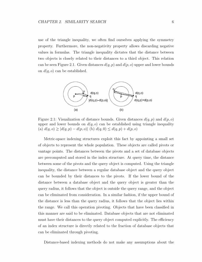
values in formulas. The triangle inequality dictates that the distance between
two objects is closely related to their distances to a third object. This relation
can be seen Figure 2.1. Given distances d(q, p) and d(p, o) upper and lower bounds
on d(q, o) can be established.
Figure 2.1: Visualization of distance bounds. Given distances d(q, p) and d(p, o)upper and lower bounds on d(q, o) can be established using triangle inequality(a) d(q, o) ≥ |d(q, p)− d(p, o)| (b) d(q, 0) ≤ d(q, p) + d(p, o)
Metric-space indexing structures exploit this fact by appointing a small set
of objects to represent the whole population. These objects are called pivots or
vantage points. The distances between the pivots and a set of database objects
are precomputed and stored in the index structure. At query time, the distance
between some of the pivots and the query object is computed. Using the triangle
inequality, the distance between a regular database object and the query object
can be bounded by their distances to the pivots. If the lower bound of the
distance between a database object and the query object is greater than the
query radius, it follows that the object is outside the query range, and the object
can be eliminated from consideration. In a similar fashion, if the upper bound of
the distance is less than the query radius, it follows that the object lies within
the range. We call this operation pivoting. Objects that have been classified in
this manner are said to be eliminated. Database objects that are not eliminated
must have their distances to the query object computed explicitly. The efficiency
of an index structure is directly related to the fraction of database objects that
can be eliminated through pivoting.
Distance-based indexing methods do not make any assumptions about the

CHAPTER 2. SIMILARITY SEARCH 7
internal structure about objects as long as distance function is defined over all
pair of objects in the collection. This level of abstraction enables us the capability
of capturing a large variety of similarity search applications. It provides a natural
and intuitive way to approach a problem. For example, the distance between two
character strings may easily be determined by the edit distance, which is a metric
[53]. On the other side, this level of abstraction eliminates some constraints which
could be useful in building indexes. For example, vector-based methods can
enhance efficiency by processing the dimensions of the vector one at a time. An
example of this is incremental distance computation [3], where the distance of the
query object to a bounding box is computed one dimension at a time. Another
example is the TV-tree [55]. In the TV-tree, new dimensions are introduced only
as they are needed.
The advantage of distance-based indexing methods is that once the index has
been built, similarity queries can often be performed with a significantly lower
number of distance computations than a sequential scan of the entire dataset, as
would be the case if no index exists. Another advantage over the multidimen-
sional indexing methods is that different distance metrics can be defined objects
and used to index them. Of course, in situations where we may want to apply
several different distance metrics, then distance-based indexing techniques have
the drawback of requiring that the index be rebuilt for each different distance
metric.
There are two main approaches when only distance functions are used in
similarity search. First method is to derive artificial features based on inter object
distances (e.g., methods described in [22, 42, 57, 89]). In these approaches, goal is
to find a mapping F that is defined for all elements of S and query objects which
maps original objects to points in k-dimensional space. New distance function
de defined in k-dimensional space should be as close as possible original distance
function d. The advantage of this approach is that it replaces original function
d with a new function de which is expected to be much less expensive. Another
advantage of this approach is that after mapping new points can be indexed using
multidimensional indexes. These methods are known as embedding methods and
they are also applicable if objects are represented as feature vectors. Advantage

CHAPTER 2. SIMILARITY SEARCH 8
of using embedding methods on features vectors is reduction in the number of
dimensions, if the dimensions of newly mapped space k, is smaller than original
dimensions of feature vector.
An important constraint on embedding methods is that the mapping F should
be contractive [39], which implies that it does not increase the distances between
objects. That is, de(F (o1), F (o2)) ≤ d(o1, o2)∀o1, o2 ∈ S. This property ensures
that there will be no incorrect elimination of objects when processing query using
new mapped space and new distance function. Results are later refined using d
(e.g., [48, 79]).
Another approach which is used when only distance functions are known is
to index objects with respect to their distances from a few selected objects called
pivots. Almost all existing index structures for metric similarity search are built
around the concept of pivoting. They differ in the way they select pivots, which
objects are associated with each pivot, how the pivot distances will be organized
and how pivots separate objects. These differences also affect how the querying
process will be carried out.
Deciding how pivots partition data is also a differentiating factor among sim-
ilarity search algorithms. [85] identified two basic partitioning schemes, ball par-
titioning and generalized hyperplane partitioning.
Figure 2.2: Possible partitioning of a set of objects. (a)ball partitioning and (b)generalized hyperplane partitioning.
In ball partitioning, the data set is partitioned based on distances from one

CHAPTER 2. SIMILARITY SEARCH 9
distinguished object, sometimes called a vantage point [93], that is, into the subset
that is inside and the subset that is outside a ball around the object (e.g., Figure
2.2(a)).
In generalized hyperplane partitioning, two distinguished objects a and b are
chosen and the data set is partitioned based on which of the two distinguished
objects is the closest, that is, all the objects in subset A are closer to a than to
b, while the objects in subset B are closer to b (e.g., Figure 2.2(b)).
2.2 Survey on Related Work
Some of the earliest distance-based indexing methods are due to [14], but most
of the work in this area has taken place in the past decades. Typical of distance
based indexing structures are metric trees [85], which are binary trees that result
in recursively partitioning a data set into two subsets at each node. The VP-tree
[93] stands out as one requiring only a small amount of memory and being able
to be constructed efficiently. However it is inferior to others in terms of query
performance, including methods like the MVP-tree [9], and GNAT [10], both of
which improve performance at the cost of greater space and construction time.
The M-tree [17] and Slim-tree [44] are disk-based structures, and support
dynamic manipulations on the index while maintaining the balance of the tree.
In order to be able to efficiently handle split and merge operations, however,
they keep less precise data than the comparable GNAT structure. This results in
poorer query performance.
While most distance based indexing structures are variations on and/or exten-
sions of metric trees, there are also other approaches. Several methods based on
distance matrices have been designed [65, 87, 88]. In these methods, all or some of
the distances between the objects in the data set are precomputed. Then, when
evaluating queries, once we have computed the actual distances of some of the
objects from the query object, the distances of the other objects can be estimated
based on the precomputed distances. Clearly, these distance matrix methods do

CHAPTER 2. SIMILARITY SEARCH 10
not form a hierarchical partitioning of the data set, but combinations of such
methods and metric tree-like structures have been proposed [64]. The SA-tree
[66] is another departure from metric trees, inspired by the Voronoi diagram. In
essence, the SA-tree records a portion of the Delaunay graph of the data set, a
graph whose vertices are the Voronoi cells, with edges between adjacent cells.
Tree structures typically only allow an object to have as many pivots as the
height of the tree. This may not be satisfactory for difficult distributions and
queries. For this reason tree-based structures are not flexible enough to provide
greater elimination power when needed. In contrast, vantage point structures
like LAESA [65], Spaghettis [15] and FQA [16] represent another family of solu-
tions. They use more space and construction time, but provide greater efficiency
at query time. Although other tree structures also have some parameters that
can be adjusted, their improvements are not as pervasive or as dramatic. The
shortcomings of vantage points-based methods are the extra computational over-
head that they incur, higher construction costs, and higher space usage. If they
are allowed to use a sufficient number of pivots, these methods have been shown
to outperform other methods in terms of the number of distance computations
performed. Some of the structures in this family offer some improvements to the
common problems of high space and construction time. The Spaghettis structure
reduces computational overhead but uses more space than the common approach.
The FQA also reduces overhead, but it uses less precision in the distance informa-
tion it stores, resulting in reduced performance in terms of the number of distance
computations.
Further material on similarity search methods can be found at [66] and [38]
which are very good surveys on similarity search.
In the following sections we report similarity search methods under three broad
categories: Clustering-based methods, local pivot-based methods, and vantage
points-based methods.

CHAPTER 2. SIMILARITY SEARCH 11
2.2.1 Clustering-Based Methods
The basic theme behind clustering-based methods is the use of a hierarchical,
tree-based decomposition of the space, where the subtrees are designed to group
close objects together. We also observe that each subtree is represented by a
single object from the database that is ideally located near the center of the
group of objects stored in this subtree.
J. Uhlmann [85] defined the gh-tree, short for generalized hyperplane tree, as
one of the first examples in this category. The idea is to pick two objects from
the current subset as representatives, and partition the rest of the set into two
classes, depending on which representative is closer.
The GNAT tree, presented by S. Brin [10] is a generalization of the gh-tree,
where there are more than two representatives. A simple algorithm is given to
pick the representatives. According to the algorithm, if we are to select k repre-
sentatives, we first pick 3 · k points randomly. Then, starting with an initial set
consisting of one random representative, we incrementally grow the set by adding
the point that maximizes the minimum distance to the other representatives.
In addition to its representatives, each node can also maintain the radius of the
associated region, that is, the maximum distance of the objects inside a represen-
tatives region. This method was used in the M-tree (described below). Another
enhancement would be to include the distances between the representatives as
well. An even more precise way is used in the GNAT tree. Every representative
stores the minimum and maximum distances to the objects in every other subset.
The performance of GNAT, in the best case, has been reported to make more
than a factor of 6 fewer distance computations than the VP-tree, while requiring
about a factor of 14 more in distance computations in its construction. How-
ever, it was reported to be worse than the VP-tree in some cases. The original
study [10] also showed that GNAT was outperformed by a variant of the vantage
points structure, although no data was given about the parameters used in the
construction of this structure. Recent experiments presented by [66], [16] show
CHAPTER 2. SIMILARITY SEARCH 12
indeed that GNAT performs consistently worse than variants of vantage points
structures in terms of number of distance computations, while it consumes less
space and has less computational overhead.
The M-tree [17] is designed to be a dynamic structure, with emphasis being
paid to the structures ability to perform queries efficiently and to optimize I/O
performance after a sequence of data insertions. Similar to SS-tree [90], it keeps
the distance to the farthest object in a subtree. Maintaining the radius of the
representative objects allows it to easily reorganize disk blocks. Splitting a node
involves selecting two new representatives and redistributing objects associated
with this node among these two new nodes. The M-tree considers all possibilities
for a split and chooses the one with tightest covering radius.
The Slim-tree [44] employs a more efficient splitting method. The minimum
spanning tree of the objects is generated and the longest arcs of the spanning tree
is removed partition the set of objects into two subsets.
2.2.2 Local Pivot-Based Methods
The structures in this category are also tree-based, however, the partitions are
based on the distances of objects to either one or two selected objects called
pivots. Objects that have similar distances to the pivots are put inside the same
subtree, but that does not necessarily mean they are in close proximity of each
other. The pivots are only used within their subset, and this is why we call
them local pivots. W. Burkhard and R. Keller [14] suggested selecting a random
object in the data set and partitioning the rest such that every object having the
same distance to the preselected object is placed in the same subset. The tree
construction continues recursively on the subset of points at the same distance.
Since their application domain produced discrete distance values, it was possible
for many points to be at the same distance.
An adaptation of the same basic idea to continuous distance values is the
VP-tree, [93]. Such a tree is defined by a branching factor. In order to construct

CHAPTER 2. SIMILARITY SEARCH 13
a vp-tree with a given branching factor k, at a given node, one of the objects is
selected as the vantage point, and the distances from the other objects to this
vantage point are calculated. Then these objects are partitioned into k groups
of roughly equal size based on these distances. In this way a node can have k
branches with each subtree having roughly m/k objects, where m denotes the
number of objects for that node. The only information that needs to be stored
is the vantage point itself, and the k − 1 distance values, denoted as cutoff[1..k],
defining the ranges of distances for each subtree.
A range query of radius r centered at a query point q is answered as follows:
at any given node, the distance d between q and the nodes vantage point is
calculated. If d is smaller than r, the vantage point is added into the result set.
For every subset i of the node defined by the cutoff values, if the interval of the
subset, [cutoff [ i− 1 ], cutoff [i]] intersects the interval [d− r, d + r], then subset
i is searched recursively.
A nice feature of the VP-tree is that it is possible to divide the space into
many divisions through a single distance calculation. As a result, when doing
a search, we need only perform one distance calculation per node. However, as
the dimensionality of the data distribution grows, it is well known that for many
distributions, the objects tend to cluster around a single distance value [5]. As
a result, almost all of the objects are at the same distance to the vantage point.
Thus, the distance to the vantage point loses its discriminating power with respect
to the objects. Another common way to describe the situation is to visualize
the situation in a 3 dimensional space, where the median spheres dividing the
branches have very similar radii, subdividing space into thin spherical shells. As
a result, objects that are grouped under same subtree tend to be spread around
the space rather being close to one another.
The MVP-tree [9] uses two vantage points per node. After partitioning the
points with one primary vantage point, the partitions are further divided by using
the second vantage point. This way, if we divide the space into m different regions
by first vantage point, we will have a total of up to m2 subsets. It should be
noted that the second vantage point uses different cutoff values for each partition

CHAPTER 2. SIMILARITY SEARCH 14
of the first vantage point. This allows the tree to maintain balance by assigning
approximately the same number of points to each subset. This occurs at the cost
of more space consumption per node. The value of this partitioning approach is
that, instead of dividing the space into very thin shells, it strives to produce more
tightly clustered subsets, while still achieving the same fanout.
The MVP-tree stores distances to two vantage points at the leaf nodes, making
it a hybrid of the vantage-point structures. It is reported to perform up to 80
2.2.3 Vantage-Point Methods
In vantage-point methods the pivots are used to control processing for the entire
set of objects instead of having local scope as they do in the previously described
methods. A subset of the objects are selected as vantage points. The distance
between the pivots and the rest of the objects are computed at initialization time
and stored in the database. At query time these precomputed distances are used
to eliminate candidates in a way that is similar to local methods. If there are
k vantage points, then the basic method performs k · n distance computations
at construction and keeps k · n distance values in the index structure. A range
query accesses these distance values to determine which objects can be eliminated
based on their distances to vantage points. Finally, a pass through all objects
not eliminated by use of pivots is performed.
Note that vantage-point methods require extra processing compared to local
methods, where determination of the partition at a node is done only for the
objects covered by the node. Local methods require storage that is only linear in
the database size, whereas vantage-point methods require O(k · n) storage.
A powerful aspect of these methods is that it is possible to use as many
pivots as desired at the cost of construction time, which results in higher storage
requirements and extra preprocessing time. Nonetheless, this additional effort
and space can yield progressively better query performance in terms of the number
of distance computations.

CHAPTER 2. SIMILARITY SEARCH 15
The first vantage-point structure that appeared in literature was LAESA [65],
as a special case of AESA [87]. There have been some improvements over the
basic LAESA algorithm, such as keeping distances to the vantage points sorted
and doing binary searches to identify which objects can be eliminated from con-
sideration [67].
The TLAESA structure [64] was proposed as a hybrid method between the
LAESA and the gh-tree. The pivots are organized as in a gh-tree, but a distance
matrix is also used to provide lower bounds for the distance of the query object to
the node representatives. Their experiments were performed in low dimensions,
and although were superior to LAESA in terms of total CPU cost, it was inferior
in terms of the number of distance computations.
The Spaghettis structure [15] was introduced as a method designed to further
decrease computational overhead. Here the distances are sorted in a similar
fashion. In addition, every distance has a pointer for the same objects distance in
the next array of distances. As done in the case of sorted distances, the feasible
ranges are computed for each array using binary search. For each point, its path
starting from first array is traced using the pointers. Once the object falls out
of range in any of the arrays, we may infer that the object cannot lie within the
query region.
The Fixed Queries Array (FQA) [16] is one of the recent global pivot-based
methods. It sorts the points according to their distances to the first vantage
point, then on the second, and so on. It decreases the precision with which
distances are measured, for otherwise the points effectively would be sorted only
in their distance to the first pivot. Using this sorted structure, the query algorithm
performs binary searches within each distance range. The first pivot is processed
as in the sorted-array approach, after that, for each range of objects that has the
same discretized distance to the first vantage point, we perform a binary search
to find the range that is valid for the second pivot. The search continues in this
fashion performing binary searches within ranges.
FQA is unique among vantage-point methods that are designed to reduce com-
putational overhead in that it does not require any additional storage. However

CHAPTER 2. SIMILARITY SEARCH 16
it does not work very well if too many bits are used for the distance values, since
this would require that the structure be sorted only by the first pivot. This cre-
ates an additional trade-off between the number of bits used for distance storage
and extra CPU processing time needed. This comes in addition to the trade-o
between number of bits and query performance in terms of distance computa-
tions. Their experiments show great improvements in low dimensions, but for 20
dimensional data for a database of one million objects, they estimate FQA would
take only 37.6
2.3 KVP Algorithm
In this section KVP structure [18], will be introduced in detail. This structure
is unique since it improves both the storage and computational overhead of the
classical vantage-points approach. The KVP structure offers a number of benefits:
1. It is a simple data structure and can be implemented relatively easily.
2. It can support dynamic operations like insertion and deletion.
3. It is easily adapted for use as a disk-based structure and its access patterns
minimize the number of disk-seek operations.
4. Queries may be executed in parallel.
2.3.1 The KVP Structure
In vantage points all pivots are kept in structure even though not all of them
may be useful in query evaluation. In [18], it is reported that it is desirable to
use pivots that are particularly close to the query object. Similarly, a pivot to
be more effective for objects that are close to or distant from it. This suggest an
improvement over keeping all pivots, at index creation time, one can find pivots
that are more close or distant to a object, and choose to keep only the distances
to these promising pivots.
CHAPTER 2. SIMILARITY SEARCH 17
This is indeed what is done with KVP, the distance relations between the
pivots and database elements are computed beforehand at construction time.
In addition to reducing CPU overhead by first processing the most promising
pivots, one can eliminate distance computations to the less promising pivots, thus
decreasing the space requirements. There are two ways this can be implemented.
One way would involve the usual layout, where every pivot stores an array of
distances to all the database objects. The object distances can be sorted so that
binary search can be used to quickly determine set of objects that are eliminated.
Another way to implement the basic idea is to have a collection of object entries,
where each object entry stores the distances to its selected pivots. The benefit
of this latter approach is that it is very easy to insert or delete objects from the
database, since there is no global data structure that keeps information about the
objects. KVP takes the second approach. Figure 2.3 illustrates the approach.
Other than the fact that KVP only stores a subset of pivot distances, the way
it processes queries is identical to the classical global pivot-based method. For
each database object it maintains a lower and upper bound for the distance to
the query object. Each pivot is used to attempt to tighten these bounds. After
processing all possible pivot distances, if the bounds are good enough to either
discard the object as out of the query range, or prove that it is within the query
range, one avoids computing the actual distance between the object and the query
object. Otherwise this distance is computed.
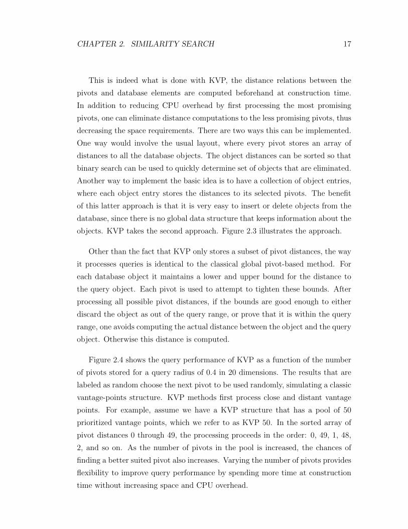
Figure 2.4 shows the query performance of KVP as a function of the number
of pivots stored for a query radius of 0.4 in 20 dimensions. The results that are
labeled as random choose the next pivot to be used randomly, simulating a classic
vantage-points structure. KVP methods first process close and distant vantage
points. For example, assume we have a KVP structure that has a pool of 50
prioritized vantage points, which we refer to as KVP 50. In the sorted array of
pivot distances 0 through 49, the processing proceeds in the order: 0, 49, 1, 48,
2, and so on. As the number of pivots in the pool is increased, the chances of
finding a better suited pivot also increases. Varying the number of pivots provides
flexibility to improve query performance by spending more time at construction
time without increasing space and CPU overhead.

CHAPTER 2. SIMILARITY SEARCH 18
Figure 2.3: A sample database of 9 vectors in 2-dimensional space, and an ex-ample of the KVP structure on this database that keeps 2 distance values perdatabase object. (a) The location of objects. Boxes represent objects that havebeen selected as pivots. (b) The distance matrix between pivots and regulardatabase objects. For each object, the 2 most promising pivot distances are se-lected to be stored in KVP (indicated by using gray background color). (c) Thefirst three object entries in the KVP. Each object entry keeps the id of the object,and an array of pivot distances.
As seen from the graphs that KVP, can eliminate database objects much faster
than the classic approach.
2.3.2 Secondary Storage
Access patterns of pivot-based structures are targeted toward minimizing CPU
time, but they are not always suitable to be stored on disk. For example, per-
forming binary search in secondary storage is expensive as it involves many seek

CHAPTER 2. SIMILARITY SEARCH 19
Figure 2.4: Query performance of the KVP structure, for vectors uniformly dis-tributed in 20 dimensions.
operations. Disks are much better at performing sequential scans. The KVP
structure is quite amenable for data that are stored on disk. It only requires a
sequential scan of distance values. It does not involve a heavy processing burden,
so processing time does not dominate over I/O time. It requires relatively little
memory, since only the vantage objects, the query object, and the distance vector
of the processed object is needed.
2.3.3 Memory Usage
KVP and its variants HKvp and EcKvp store fewer distance values than the clas-
sic vantage-point methods [18]. Depending on the parameters of KVP structure,
memory usage of KVP changes. KVP structure keeps tracks of indexes used in
structure. Also for each object a subset of pivots is selected, and distance from

CHAPTER 2. SIMILARITY SEARCH 20
object to selected pivots is precomputed and stored.
For object collection of n objects, if bd bits are used for distance values and
bi bits are used for indexes of pivots, and assuming npivot selected in index con-
struction with npivotlimit limit per object, memory usage of KVP is mKV P ,
mKV P = n× (npivotlimit × (bd + bi)) + npivot ∗ bi
As with FQA, KVP can decrease memory consumption by discretization, so
that fewer bits are used for the distance values. Consider its simplest form where
the intervals have equal width, using b bits in a metric space where the maximum
distance is Dmax. This will map distances into buckets of width Dw where
Dw = Dmax
2b
Since all the distances in the same bucket will be assigned the same distance
value, the maximum error will be Dw per distance value. Assuming query objects
are distributed uniformly, we can approximate the error toDw/2 .
Therefore, query process is modified to use r+ Dmax
2, instead of r and rest of al-
gorithm stays same. This discretization can improve memory usage considerably,
since can be very large n.
2.3.4 Comparison of KVP and Tree-Based Structures
Using a KVP structure, one can easily vary a number of parameters, including
the construction cost, the number of pivots used per object, the number of pivots
stored per object, the number of pivots processed at query time per object, and
the number of bits used per distance value.
In a sense, it is possible to view most of the existing structures as variants of
the vantage point-based methods. For example in a VP-tree with a branching fac-
tor of k, there is one pivot per node, all the objects in subtrees can be eliminated
with their distances to this pivot, and number of branches have an affect similar
to the number of bits used. For a database object, there are approximately as
CHAPTER 2. SIMILARITY SEARCH 21
many pivots as the height of the tree. This view explains why changing k in the
VP-tree has little affect on query performance, since as k increases and pivots
become more precise (which is similar to using more bits), the height of the tree
becomes shorter and there are fewer pivots per database object. A major problem
with the VP-tree is that the only data that is used are the cutoff values. The
individual distances of objects to the pivots are computed but then discarded.
From the perspective of vantage points, it is also easier to see why GNAT
with branching factor k improves on the VP-tree. In GNAT, there are k pivots
per node, and the distance ranges of k subtree to these pivots are stored. One
slight disadvantage of GNAT is that ranges of distances to a pivot can overlap.
However, instead of having just one pivot per one, objects in GNAT make use of
k pivots.
Tree-based methods have two advantages over the classical vantage points
methods. Whereas a pivoting operation involves one object in vantage points,
it usually involves groups of objects in tree-based structures. This is something
that only cause increase on the CPU overhead, and has a negative impact on
the number of distance computations. Secondly, tree-based methods attempt to
divide the space into clusters in order to benefit from the locality of pivots. This
is similar to what priority vantage points and KVP try to accomplish. While
tree structures have varying degrees of success in clustering similar objects to-
gether, KVP takes a direct approach and precisely computes the closest pivots.
In addition, KVP properly makes use of far pivots as well.
Chapter 3
General Purpose Computing On
GPU
Recent developments on graphics chips, known generically as Graphics Processing
Units or GPUs, have provided a quite powerful computational units. Researchers
and developers have become interested in utilizing this power for general purpose
computing, an effort known collectively as GPGPU (for General Purpose com-
puting on the GPU). In this section we summarize the efforts in field of GPGPU,
give an overview of the techniques and computational building blocks used to
map general purpose computation to graphics hardware, and survey the various
general purpose computing tasks to which GPUs have been applied. A quite good
survey on this field is provided by Owens et al. [71], which this section is based.
Recent graphics architectures provide tremendous memory bandwidth and
computational horsepower. For example, the flagship ATI Radeon HD 5970
($625 as of January 2010) boasts 256.0 GB/sec memory bandwidth; with 4.64
TeraFLOPS theoretical single precision processing power. Similarly competitor
NVIDIA’s flagship product GeForce 295 GTX ($475 as of January 2010) has
223.8 GB/sec memory bandwidth. GPUs also use advanced processor technol-
ogy; for example, the ATI HD 5970 contains 4.3 billion transistors and is built
on a 40-nanometer fabrication process.
22

CHAPTER 3. GENERAL PURPOSE COMPUTING ON GPU 23
Graphics hardware is fast and getting faster quickly. In fact graphics hard-
ware performance increasing more rapidly than that of CPUs. The disparity can
be attributed to fundamental architectural differences: CPUs are optimized for
high performance on sequential code, with many transistors dedicated to extract-
ing instruction-level parallelism with techniques such as branch prediction and
out-of-order execution. On the other hand, the highly data-parallel nature of
graphics computations enables GPUs to use additional transistors more directly
for computation, achieving higher arithmetic intensity with the same transistor
count.
Modern graphics architectures have become flexible as well as powerful. Early
GPUs were fixed-function pipelines whose output was limited to 8-bit-per-channel
color values, whereas modern GPUs now include fully programmable processing
units that support vectorized floating point operations on values stored at full
IEEE single precision (but note that the arithmetic operations themselves are not
yet perfectly IEEE-compliant). High level languages have emerged to support the
new programmability of the vertex and pixel pipelines [12, 61, 62]. Additional
levels of programmability are emerging with every major generation of GPU
(roughly every 18 months). For example, current generation GPUs introduced
vertex texture access, full branching support in the vertex pipeline, and limited
branching capability in the fragment pipeline. The next generation will expand
on these changes and add geometry shaders, or programmable primitive assembly,
bringing flexibility to an entirely new stage in the pipeline [6]. The raw speed,
increasing precision, and rapidly expanding programmability of GPUs make them
an attractive platform for general purpose computation.
Yet the GPU is hardly a computational panacea. Its arithmetic power results
from a highly specialized architecture, evolved and tuned over years to extract
maximum performance on the highly parallel tasks of traditional computer graph-
ics. The increasing flexibility of GPUs, coupled with some ingenious uses of that
flexibility by GPGPU developers, has enabled many applications outside the orig-
inal narrow tasks for which GPUs were originally designed, but many applications
still exist for which GPUs are not (and likely never will be) well suited. Word
processing, for example, is a classic example of a pointer chasing application,

CHAPTER 3. GENERAL PURPOSE COMPUTING ON GPU 24
dominated by memory communication and difficult to parallelize.
Todays GPUs also lack some fundamental computing constructs, such as effi-
cient scatter memory operations (i.e., indexed write array operations) and integer
data operands. The lack of integers and associated operations such as bit-shifts
and bitwise logical operations (AND, OR, XOR, NOT) makes GPUs ill-suited
for many computationally intense tasks such as cryptography (though upcoming
Direct3D 10 class hardware will add integer support and more generalized in-
structions [6]). Finally, while the recent increase in precision to 32-bit floating
point has enabled a host of GPGPU applications, 64-bit double precision arith-
metic remains a promise on the horizon. The lack of double precision hampers
or prevents GPUs from being applicable to many very large scale computational
science problems.
Furthermore, graphics hardware remains difficult to apply to non-graphics
tasks. The GPU uses an unusual programming model, so effective GPGPU pro-
gramming is not simply a matter of learning a new language. Instead, the com-
putation must be recast into graphics terms by a programmer familiar with the
design, limitations, and evolution of the underlying hardware. Today, harnessing
the power of a GPU for scientific or general purpose computation often requires
a concerted effort by experts in both computer graphics and in the particular
computational domain. But despite the programming challenges, the potential
benefits, a leap forward in computing capability and a growth curve much faster
than traditional CPUs are too large to ignore.
3.1 Overview Of Graphics Hardware
In this section we will outline the evolution of the GPU and describe its current
hardware and software.
3D graphics applications require high computation rates and exhibit substan-
tial parallelism which differentiate it from more general computation domains.
Graphic cards are designed to take advantage of the native parallelism in the

CHAPTER 3. GENERAL PURPOSE COMPUTING ON GPU 25
application, allowing higher performance on graphics applications than can be
obtained on more traditional microprocessors.
All of today’s commodity GPUs structure their graphics computation in a
similar organization called the graphics pipeline. This pipeline is designed to allow
hardware implementations to maintain high computation rates through parallel
execution. The pipeline is divided into several stages. All geometric primitives
pass through each stage: vertex operations, primitive assembly, rasterization,
fragment operations, and composition into a final image. In hardware, each stage
is implemented as a separate piece of hardware on the GPU in what is termed a
task parallel machine organization. Figure 3.1 shows the pipeline stages in current
GPUs. For more detail on GPU hardware and the graphics pipeline, NVIDIA’s
GeForce 6 series of GPUs is described by Kilgariff and Fernando [47]. From
a software perspective, the OpenGL Programming Guide provides an excellent
reference [69].
Figure 3.1: The modern graphics hardware pipeline. The vertex and fragmentprocessor stages are both programmable by the user.

CHAPTER 3. GENERAL PURPOSE COMPUTING ON GPU 26
3.1.1 Programmable hardware
The graphics pipeline described above was historically a fixed function pipeline,
where the limited number of operations available at each stage of the graphics
pipeline were hardwired for specific tasks. However, the success of off-line ren-
dering systems such as Pixars RenderMan [86] demonstrated the benefit of more
flexible operations, particularly in the areas of lighting and shading. Instead
of limiting lighting and shading operations to a few fixed functions, RenderMan
evaluated a user defined shader program on each primitive, with impressive visual
results.
Over the past seven years, graphics vendors have transformed the fixed func-
tion pipeline into a more flexible programmable pipeline. This effort has been
primarily concentrated on two stages of the graphics pipeline: the vertex stage
and the fragment stage. In the fixed function pipeline, the vertex stage included
operations on vertices such as transformations and lighting calculations. In the
programmable pipeline, these fixed function operations are replaced with a user
defined vertex program. Similarly, the fixed function operations on fragments
that determine the fragment’s color are replaced with a user defined fragment
program.
Each new generation of GPUs has increased the functionality and generality
of these two programmable stages. 1999 marked the introduction of the first pro-
grammable stage, NVIDIA’s register combiner operations that allowed a limited
combination of texture and interpolated color values to compute a fragment color.
In 2002, ATI’s Radeon 9700 led the transition to floating point computation in
the fragment pipeline.
The vital step for enabling general purpose computation on GPUs was the
introduction of fully programmable hardware and an assembly language for spec-
ifying programs to run on each vertex [56] or fragment. This programmable shader
hardware is explicitly designed to process multiple data parallel primitives at the
same time. In general, these programmable stages input a limited number of
32-bit floating point 4-vectors. The vertex stage outputs a limited number of

CHAPTER 3. GENERAL PURPOSE COMPUTING ON GPU 27
32-bit floating point 4-vectors that will be interpolated by the rasterizer; the
fragment stage outputs up to 4 floating point 4-vectors, typically colors. Each
programmable stage can access constant registers across all primitives and also
read-write registers per primitive. The programmable stages have limits on their
numbers of inputs, outputs, constants, registers, and instructions; with each new
revision of the vertex shader and pixel [fragment] shader standard, these limits
have increased.
GPUs typically have multiple vertex and fragment processors. Fragment pro-
cessors have the ability to fetch data from textures, so they are capable of memory
gather. However, the output address of a fragment is always determined before
the fragment is processed, and the processor cannot change the output location
of a pixel. Vertex processors recently acquired texture capabilities, and they are
capable of changing the position of input vertices, which ultimately affects where
in the image pixels will be drawn. Thus, vertex processors are capable of both
gather and scatter. Unfortunately, vertex scatter can lead to memory and ras-
terization coherence issues further down the pipeline. Combined with the lower
performance of vertex processors, this limits the utility of vertex scatter in current
GPUs.
3.2 GPU Programming Model
GPUs are a compelling solution for applications that require high arithmetic rates
and data bandwidths. GPUs achieve this high performance through data paral-
lelism, which requires a programming model distinct from the traditional CPU
sequential programming model. In this section, we briefly introduce the GPU
programming model using both graphics API terminology and the terminology
of the more abstract stream programming model, because both are common in
the literature.
The stream programming model exposes the parallelism and communication
CHAPTER 3. GENERAL PURPOSE COMPUTING ON GPU 28
patterns inherent in the application by structuring data into streams and ex-
pressing computation as arithmetic kernels that operate on streams. Owens [70]
discuss the stream programming model in the context of graphics hardware, and
the Brook programming system [12] offers a stream programming system for
GPUs.
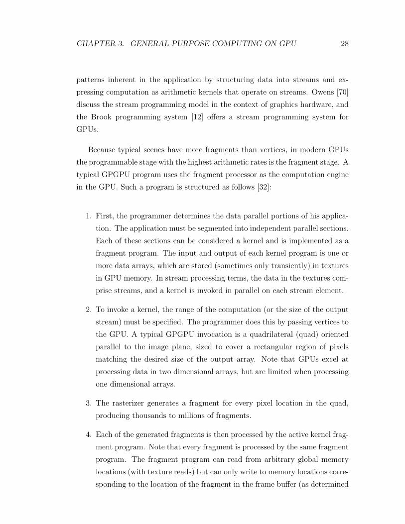
Because typical scenes have more fragments than vertices, in modern GPUs
the programmable stage with the highest arithmetic rates is the fragment stage. A
typical GPGPU program uses the fragment processor as the computation engine
in the GPU. Such a program is structured as follows [32]:
1. First, the programmer determines the data parallel portions of his applica-
tion. The application must be segmented into independent parallel sections.
Each of these sections can be considered a kernel and is implemented as a
fragment program. The input and output of each kernel program is one or
more data arrays, which are stored (sometimes only transiently) in textures
in GPU memory. In stream processing terms, the data in the textures com-
prise streams, and a kernel is invoked in parallel on each stream element.
2. To invoke a kernel, the range of the computation (or the size of the output
stream) must be specified. The programmer does this by passing vertices to
the GPU. A typical GPGPU invocation is a quadrilateral (quad) oriented
parallel to the image plane, sized to cover a rectangular region of pixels
matching the desired size of the output array. Note that GPUs excel at
processing data in two dimensional arrays, but are limited when processing
one dimensional arrays.
3. The rasterizer generates a fragment for every pixel location in the quad,
producing thousands to millions of fragments.
4. Each of the generated fragments is then processed by the active kernel frag-
ment program. Note that every fragment is processed by the same fragment
program. The fragment program can read from arbitrary global memory
locations (with texture reads) but can only write to memory locations corre-
sponding to the location of the fragment in the frame buffer (as determined

CHAPTER 3. GENERAL PURPOSE COMPUTING ON GPU 29
by the rasterizer). The domain of the computation is specified for each in-
put texture (stream) by specifying texture coordinates at each of the input
vertices, which are then interpolated at each generated fragment. Texture
coordinates can be specified independently for each input texture, and can
also be computed on the fly in the fragment program, allowing arbitrary
memory addressing.
5. The output of the fragment program is a value (or vector of values) per
fragment. This output may be the final result of the application, or it may
be stored as a texture and then used in additional computations. Com-
plex applications may require several or even dozens of passes (multipass)
through the pipeline.
While the complexity of a single pass through the pipeline may be limited
(for example, by the number of instructions, by the number of outputs allowed
per pass, or by the limited control complexity allowed in a single pass), using
multiple passes allows the implementation of programs of arbitrary complexity.
3.2.1 GPU Program Flow
Flow control is a fundamental concept in computation. Branching and looping
are such basic concepts that it can be daunting to write software for a platform
that supports them to only a limited extent. The latest GPUs support vertex and
fragment program branching in multiple forms, but their highly parallel nature
requires care in how they are used. This section surveys some of the limitations
of branching on current GPUs and describes a variety of techniques for iteration
and decision making in GPGPU programs. Harris and Buck [33] provide more
detail on GPU flow control.
CHAPTER 3. GENERAL PURPOSE COMPUTING ON GPU 30
3.2.1.1 Hardware mechanisms for flow control
There are three basic implementations of data parallel branching in use on current
GPUs: predication, MIMD branching, and SIMD branching.
Architectures that support only predication do not have true data dependent
branch instructions. Instead, the GPU evaluates both sides of the branch and
then discards one of the results based on the value of the Boolean branch condi-
tion. The disadvantage of predication is that evaluating both sides of the branch
can be costly, but not all current GPUs have true data dependent branching
support. The compiler for high level shading languages like Cg or the OpenGL
Shading Language automatically generates predicated assembly language instruc-
tions if the target GPU supports only predication for flow control.
In Multiple Instruction Multiple Data (MIMD) architectures that support
branching, different processors can follow different paths through the program.
In Single Instruction Multiple Data (SIMD) architectures, all active processors
must execute the same instructions at the same time. The only MIMD processors
in a current GPU are the vertex processors of the NVIDIA GeForce 6 and 7 series
and NV40 and G70 based Quadro GPUs. Classifying GPU fragment processors
is more difficult. The programming model is effectively Single Program Multiple
Data (SPMD), meaning that threads (pixels) can take different branches. How-
ever, in terms of architecture and performance, fragment processors on current
GPUs process pixels in SIMD groups. Within a SIMD group, when evaluation
of the branch condition is identical for all pixels in the group, only the taken
side of the branch must be evaluated. However, if one or more of the processors
evaluates the branch condition differently, then both sides must be evaluated and
the results predicated. As a result, divergence in the branching of simultaneously
processed fragments can lead to reduced performance.

CHAPTER 3. GENERAL PURPOSE COMPUTING ON GPU 31
3.2.1.2 Moving branching up the pipeline
Because explicit branching can hamper performance on GPUs, it is useful to have
multiple techniques to reduce the cost of branching. A useful strategy is to move
flow control decisions up the pipeline to an earlier stage where they can be more
efficiently evaluated.
Static Branch Resolution On the GPU, as on the CPU, avoiding branching
inside inner loops is beneficial. For example, when evaluating a partial differential
equation (PDE) on a discrete spatial grid, an efficient implementation divides
the processing into multiple loops: one over the interior of the grid, excluding
boundary cells, and one or more over the boundary edges. This static branch
resolution results in loops that contain efficient code without branches. (In stream
processing terminology, this technique is typically referred to as the division of
a stream into substreams.) On the GPU, the computation is divided into two
fragment programs: one for interior cells and one for boundary cells. The interior
program is applied to the fragments of a quad drawn over all but the outer one
pixel edge of the output buffer. The boundary program is applied to fragments
of lines drawn over the edge pixels. Static branch resolution is further discussed
by Goodnight et al. [25].
Z-Cull Precomputed branch results can be taken a step further by using an-
other GPU feature to entirely skip unnecessary work. Modern GPUs have a
number of features designed to avoid shading pixels that will not be seen. One
of these is Z-cull. Z-cull is a hierarchical technique for comparing the depth (Z)
of an incoming block of fragments with the depth of the corresponding block of
fragments in the Z-buffer. If the incoming fragments will all fail the depth test,
then they are discarded before their pixel colors are calculated in the fragment
processor. Thus, only fragments that pass the depth test are processed, work is
saved, and the application runs faster. In fluid simulation, land locked obstacle
cells can be masked with a z-value of zero so that all fluid simulation computa-
tions will be skipped for those cells. If the obstacles are fairly large, then a lot
of work is saved by not processing these cells. Harris and Buck provide pseudo
code [33] for the technique.

CHAPTER 3. GENERAL PURPOSE COMPUTING ON GPU 32
Data Dependent Looping With Occlusion Queries Another GPU feature de-
signed to avoid drawing what is not visible is the hardware occlusion query (OQ).
This feature provides the ability to query the number of pixels updated by a ren-
dering call. These queries are pipelined, which means that they provide a way
to get a limited amount of data (an integer count) back from the GPU without
stalling the pipeline (which would occur when actual pixels are read back). Be-
cause GPGPU applications almost always draw quads with known pixel coverage,
OQ can be used with fragment kill functionality to get a count of fragments up-
dated and killed. This allows the implementation of global decisions controlled
by the CPU based on GPU processing. Harris and Buck provide pseudo code for
the technique [33].
3.2.2 GPU Programming Systems
In this section we look at the high level languages that have been developed for
GPU programming, and the debugging tools that are available for GPU pro-
grammers. Code profiling and tuning tends to be a very architecture specific
task. GPU architectures have evolved very rapidly, making profiling and tuning
primarily the domain of the GPU manufacturer. As such, we will not discuss
code profiling tools in this section.
3.2.2.1 High Level Shading Languages
Most high level GPU programming languages today share one thing in common:
they are designed around the idea that GPUs generate pictures. As such, the high
level programming languages are often referred to as shading languages. That
is, they are a high level language that compiles a shader program into a vertex
shader and a fragment shader to produce the image described by the program.
Cg [61], HLSL, and the OpenGL Shading Language all abstract the capabil-
ities of the underlying GPU and allow the programmer to write GPU programs
in a more familiar C-like programming language. They do not stray far from
CHAPTER 3. GENERAL PURPOSE COMPUTING ON GPU 33
their origins as languages designed to shade polygons. All retain graphics specific
constructs: vertices, fragments, textures, etc. Cg and HLSL provide abstractions
that are very close to the hardware, with instruction sets that expand as the
underlying hardware capabilities expand. The OpenGL Shading Language was
designed looking a bit further out, with many language features (e.g. integers)
that do not directly map to hardware available today.
Sh is a shading language implemented on top of C++ [62]. Sh provides a
shader algebra for manipulating and defining procedurally parameterized shaders.
Sh manages buffers and textures, and handles shader partitioning into multiple
passes. Sh also provides a stream programming abstraction suitable for GPGPU
programming.
3.2.3 GPGPU languages and libraries
More often than not, the graphics centric nature of shading languages makes
GPGPU programming more difficult than it needs to be. As a simple example,
initiating a GPGPU computation usually involves drawing a primitive. Looking
up data from memory is done by issuing a texture fetch. The GPGPU program
may conceptually have nothing to do with drawing geometric primitives and
fetching textures, yet the shading languages described in the previous section
force the GPGPU application writer to think in terms of geometric primitives,
fragments, and textures. Instead, GPGPU algorithms are often best described as
memory and math operations, concepts much more familiar to CPU programmers.
The programming systems below attempt to provide GPGPU functionality while
hiding the GPU specific details from the programmer.
The Brook programming language extends ANSI C with concepts from stream
programming [12]. Brook can use the GPU as a compilation target. Brook
streams are conceptually similar to arrays, except all elements can be operated
on in parallel. Kernels are the functions that operate on streams. Brook auto-
matically maps kernels and streams into fragment programs and texture memory.

CHAPTER 3. GENERAL PURPOSE COMPUTING ON GPU 34
Accelerator is a system from Microsoft Research that aims to simplify GPGPU
programming by providing a high level data parallel programming model in a
library that is accessible from within traditional imperative programming lan-
guages [82]. Accelerator translates data parallel operations on the fly to GPU
pixel shaders, demonstrating significant speedups over C versions running on the
CPU.
CGiS is a data parallel programming language from the Saarland University
Compiler Design Lab with similar aims to Brook and Accelerator, but with a
slightly different approach [63]. Like Brook, CGiS provides stream data types,
but instead of explicit kernels that run on the GPU, the language invokes GPU
computation via a built in data parallel forall operator.
The Glift template library provides a generic template library designed to
simplify GPU data structure design and separate GPU algorithms from data
structures [51]. Glift defines GPU computation as parallel iteration over the
elements of a data structure. The model generalizes the stream computation
model and connects GPGPU with CPU based parallel data structure libraries
such as the Standard Template Adaptive Parallel Library (STAPL). The library
integrates with a C++, Cg, and OpenGL GPU development environment.
CUDA (an acronym for Compute Unified Device Architecture) is a parallel
computing architecture developed by NVIDIA. CUDA is the computing engine in
NVIDIA graphics processing units or GPUs that is accessible to software develop-
ers through industry standard programming languages. Programmers use ’C for
CUDA’ (C with NVIDIA extensions), compiled through a PathScale Open64 C
compiler, to code algorithms for execution on the GPU. CUDA architecture sup-
ports a range of computational interfaces including OpenCL and DirectCompute.
Third party wrappers are also available for Python, Fortran, Java and Matlab.
AMD first released its Stream Computing SDK (v1.0), in December 2007 un-
der the AMD EULA, to be run on Windows XP. The SDK includes ”Brook+”,
an AMD hardware optimized version of the Brook language developed by Stan-
ford University, itself a variant of the ANSI C (C language), open-sourced and
optimized for stream computing. The AMD Core Math Library (ACML) and

CHAPTER 3. GENERAL PURPOSE COMPUTING ON GPU 35
AMD Performance Library (APL) also be included as a part of SDK. Another
important part of the SDK, the Compute Abstraction Layer (CAL), is a software
development layer aimed for low-level access, through the CTM hardware inter-
face, to the GPU architecture for performance tuning software written in various
high-level programming languages.
Finally, the OpenCL (Open Computing Language) is a framework for writing
programs that execute across heterogeneous platforms consisting of CPUs, GPUs,
and other processors. OpenCL includes a language (based on C99) for writing
kernels (functions that execute on OpenCL devices), plus APIs that are used to
define and then control the platforms. OpenCL provides parallel computing using
task-based and data-based parallelism.
OpenCL is analogous to the open industry standards OpenGL and OpenAL,
for 3D graphics and computer audio, respectively. OpenCL extends the power
of the GPU beyond graphics (GPGPU). OpenCL is managed by the non-profit
technology consortium Khronos Group (http://www.khronos.org/opencl/).
3.2.4 Debugging tools
Support for debugging on GPUs is fairly limited, when compared with CPU. The
advent of GPGPU programming makes it clear that a GPU debugger should have
similar capabilities as traditional CPU debuggers, including variable watches, pro-
gram break points, and single-step execution. GPU programs often involve user
interaction. While a debugger does not need to run the application at full speed,
the application being debugged should maintain some degree of interactivity. A
GPU debugger should be easy to add to and remove from an existing applica-
tion, should mangle GPU state as little as possible, and should execute the debug
code on the GPU, not in a software rasterizer. Finally, a GPU debugger should
support the major GPU programming APIs and vendor-specific extensions.
There are a few different systems for debugging GPU programs available to
use, but nearly all are missing one or more of the important features that are

CHAPTER 3. GENERAL PURPOSE COMPUTING ON GPU 36
present in cpu debuggers.
gDEBugger [2] and GLIntercept [83] are tools designed to help debug OpenGL
programs. Both are able to capture and log OpenGL state from a program. gDE-
Bugger allows a programmer to set breakpoints and watch OpenGL state variables
at runtime, as well as to profile applications using GPU hardware performance
signals. There is currently no specific support for debugging shaders, but both
support runtime shader editing.
The Microsoft Shader Debugger [1], however, does provide runtime variable
watches and breakpoints for shaders. The shader debugger is integrated into the
Visual Studio IDE, and provides all the same functionality programmers are used
to for traditional programming. Unfortunately, debugging requires the shaders to
be run in software emulation rather than on the hardware. In contrast, the Apple
OpenGL Shader Builder also has a sophisticated IDE and actually runs shaders in
real time on the hardware during shader debug and edit. The downside to this tool
is that it was designed for writing shaders, not for computation. The shaders are
not run in the context of the application, but in a separate environment designed
to help facilitate shader writing.
While many of the tools mentioned so far provide a lot of useful features for
debugging, none provide any support for shader data visualization or printf-style
debugging. Sometimes this is the single most useful tool for debugging programs.
The Image Debugger [4] was among the first tools to provide this functionality by
providing a printf-like function over a region of memory. The region of memory
gets mapped to a display window, allowing a programmer to visualize any block of
memory as an image. The Image Debugger does not provide any special support
for shader programs, so programmers must write shaders such that the output
gets mapped to an output buffer for visualization.
The Shadesmith Fragment Program Debugger [74] was the first system to
automate printf-style debugging while providing basic shader debugging func-
tionality like breakpoints, program stepping, and programmable scale and bias
for the image printf. While Shadesmith represents a big step in the right direction
for GPGPU debugging, it still has many limitations, the largest of which is that

CHAPTER 3. GENERAL PURPOSE COMPUTING ON GPU 37
Shadesmith is currently limited to debugging assembly language shaders. Addi-
tionally, Shadesmith only works for OpenGL fragment programs, and provides
no support for debugging OpenGL state.
3.3 GPGPU Techniques
In this section we describe some of the building blocks of GPU computation.
3.3.1 Stream operations
There are several fundamental operations on streams that many GPGPU appli-
cations implement. These operations are: map, reduce, scatter and gather, scan,
stream filtering, sort, and search. In the following sections we define each of these
operations.
3.3.1.1 Map
Given a stream of data elements and a function, map will apply the function to
every element in the stream. The GPU implementation of map is straightforward,
and perhaps best illustrated with an example. Assume we have a stream of data
with values. We would like to compute squares of these values. A kernel to do
this would multiply each element in the stream by itself to produce the output
stream. This application of a function to an input stream is the essence of the
map operation.
3.3.1.2 Reduce
Sometimes a computation requires computing a smaller stream from a larger
input stream, possibly to a single element stream. This type of computation is

CHAPTER 3. GENERAL PURPOSE COMPUTING ON GPU 38
called a reduction. For example, a reduction can be used to compute the sum or
maximum of all the elements in a stream.
On GPUs, reductions can be performed by alternately rendering to and read-
ing from a pair of textures. On each rendering pass, the size of the output, the
computational range, is reduced by one half. In general, we can compute a re-
duction over a set of n data elements in O(nplogn) time steps using the parallel
GPU hardware (with p elements processed in one time step), compared to O(n)
time steps for a sequential reduction on the CPU. To produce each element of the
output, a fragment program reads two values, one from a corresponding location
on either half of the previous pass result buffer, and combines them using the
reduction operator (for example, addition or maximum). These passes continue
until the output is a one-by-one buffer, at which point we have our reduced re-
sult. For a two dimensional reduction, the fragment program reads four elements
from four quadrants of the input texture, and the output size is halved in both
dimensions at each step. Buck et al. describe GPU reductions in more detail in
the context of the Brook programming language [12].
3.3.1.3 Scatter and Gather
Two fundamental memory operations with which most programmers are familiar
are write and read. If the write and read operations access memory indirectly,
they are called scatter and gather respectively. A scatter operation looks like the
C code d[a] = v where the value v is being stored into the data array d at address
a. A gather operation is just the opposite of the scatter operation. The C code
for gather looks like v = d[a].
The GPU implementation of gather is essentially a dependent texture fetch
operation. A texture fetch from texture d with computed texture coordinates a
performs the indirect memory read that defines gather. Unfortunately, scatter
is not as straightforward to implement. Fragments have an implicit destination
address associated with them: their location in frame buffer memory. A scatter
operation would require that a program change the framebuffer write location of
CHAPTER 3. GENERAL PURPOSE COMPUTING ON GPU 39
a given fragment, or would require a dependent texture write operation. Since
neither of these mechanisms exist on today’s GPU, GPGPU programmers must
resort to various tricks to achieve a scatter. These tricks include rewriting the
problem in terms of gather; tagging data with final addresses during a traditional
rendering pass and then sorting the data by address to achieve an effective scatter;
and using the vertex processor to scatter (since vertex processing is inherently a
scattering operation). Buck has described these mechanisms for changing scatter
to gather in greater detail [11].
3.3.1.4 Scan
A simple and common parallel algorithmic building block is the all-prefix-sums
operation, also known as scan [37]. For each element in a sequence of elements,
prefix-sum computes the sum of all previous elements in the sequence. The
first implementation of scan on GPUs was presented by Horn and demonstrated
for the applications of collision detection and subdivision surfaces [41]. Hensley
et al. used a similar scan implementation to generate summed-area tables on
the GPU [36]. The algorithms of Horn and Hensley et al. were efficient in
the number of passes (O(log n)) executed, but required O(n log n) total work,
a factor of log n worse than the optimal sequential work complexity of O(n).
Greß et al. presented O(n) algorithms for GPUs [30]. Greß et al. construct
a list of potentially intersecting bounding box pairs and utilize scan to remove
the non-intersecting pairs. The algorithm of Sengupta et al. is notable for its
method of switching from a tree-based work-efficient algorithm to Horns brute-
force algorithm as it approaches the root of the tree. This hybrid approach more
efficiently uses all of the parallelism provided by the GPU.
3.3.1.5 Stream filtering
Many algorithms require the ability to select a subset of elements from a stream,
and discard the rest. The location and number of elements to be filtered is vari-
able and not known a priori. Example algorithms that benefit from this stream

CHAPTER 3. GENERAL PURPOSE COMPUTING ON GPU 40
filtering operation include simple data partitioning (where the algorithm only
needs to operate on stream elements with positive keys and is free to discard neg-
ative keys) and collision detection (where only objects with intersecting bounding
boxes need further computation).
Horn has described a technique called stream compaction [41] that implements
stream filtering on the GPU. Using a combination of scan and search, stream
filtering can be achieved in O(log n) passes.
3.3.1.6 Sort
A sort operation allows us to transform an unordered set of data into an or-
dered set of data. Sorting is a classic algorithmic problem that has been solved
by several different techniques on the CPU. Many of these algorithms are data-
dependent and generally require scatter operations; therefore, they are not di-
rectly applicable to a clean GPU implementation. Data-dependent operations
are difficult to implement efficiently, and scatter is not implemented for frag-
ment processors on today’s GPUs. To make efficient use of GPU resources, a
GPU-based sort should be oblivious to the input data, and should not require
scatter.
Most GPU-based sorting implementations [31, 46, 76, 75] have been based on
sorting networks. The main idea behind a sorting network is that a given network
configuration will sort input data in a fixed number of steps, regardless of the
input data. Additionally, all the nodes in the network have a fixed communication
pattern. The fixed communication pattern means the problem can be stated in
terms of gather rather than scatter, and the fixed number of stages for a given
input size means the sort can be implemented without data-dependent branching.
This yields an efficient GPU-based sort, with an overall O(nlog2n) computational
complexity.
Sorting networks can also be implemented efficiently using the texture map-
ping and blending functionalities of the GPU [29]. In each step of the sorting
network, a comparator mapping is created at each pixel on the screen and the

CHAPTER 3. GENERAL PURPOSE COMPUTING ON GPU 41
color of the pixel is compared against exactly one other pixel. The comparison
operations are implemented using the blending functionality and the comparator
mapping is implemented using the texture mapping hardware, thus entirely elimi-
nating the need for fragment programs. Govindaraju et al. have also analyzed the
cache efficiency of sorting network algorithms and presented an improved bitonic
sorting network algorithm with a better data access pattern and data layout.
The precision of the underlying sorting algorithm using comparisons with fixed-
function blending hardware is limited to the precision of the blending hardware.
For example, the current blending hardware has 16-bit floating point precision.
Alternatively, the limitation to 16-bit values on current GPUs can be alleviated
by using a single-line fragment program for evaluating the conditionals, but the
fragment program implementation on current GPUs is slightly slower than the
fixed-function pipeline.
Greß and Zachmann [31] present a novel algorithm, GPU-ABiSort, to further
enhance the sorting performance on GPUs. Their algorithm is based on an adap-
tive bitonic sorting algorithm and achieves an optimal performance of O(n log
n) for any computation time T in the range of O(log2n) ≤ T ≤ O(nlogn). The
algorithm maps well to the GPU and is able to achieve good performance on an
NVIDIA 7800 GTX GPU.
GPUs have also been used to efficiently perform 1-D and 3-D adaptive sorting
of sequences [27]. Unlike sorting network algorithms, the computational complex-
ity of adaptive sorting algorithms is dependent on the extent of disorder in the
input sequence, and work well for nearly-sorted sequences. The extent of disorder
is computed using Knuths measure of disorder. Given an input sequence I, the
measure of disorder is defined as the minimal number of elements that need to
be removed for the rest of the sequence to remain sorted. The algorithm pro-
ceeds in multiple iterations. In each iteration, the unsorted sequence is scanned
twice. In the first pass, the sequence is scanned from the last element to the
first, and an increasing sequence of elements M is constructed by comparing each
element with the current minimum. In the second pass, the sorted elements in
the increasing sequence are computed by comparing each element in M against
the current minimum in I M. The overall algorithm is simple and requires only
CHAPTER 3. GENERAL PURPOSE COMPUTING ON GPU 42
comparisons against the minimum of a set of values. The algorithm is, therefore,
useful for fast 3D visibility ordering of elements where the minimum comparisons
are implemented using the depth buffer [27].
External memory sorting algorithms are used to organize large terabyte-scale
datasets. These algorithms proceed in two phases and use limited main memory
to order the data. Govindaraju et al. [26] present a novel external memory
sorting algorithm to sort billion-record wide-key databases using a GPU. In the
first phase, GPUTeraSort pipelines the following tasks on the CPU, disk controller
and GPU: read disk asynchronously, build keys, sort using a GPU, generate runs
and write disk. In this phase, GPUTeraSort uses the data parallelism and high
memory bandwidth on GPUs to quickly sort large runs. In the second phase,
GPUTera-Sort uses a similar task pipeline to read, merge and write the runs.
GPUTeraSort offloads the compute-intensive and memory intensive tasks to the
GPU; therefore, it is able to achieve higher I/O performance and better memory
performance than CPU-only algorithms.
3.3.1.7 Search
The last stream operation we discuss, search, allows us to find a particular ele-
ment within a stream. Search can also be used to find the set of nearest neighbors
to a specified element. Nearest neighbor search is used extensively when com-
puting database queries (e.g. find the 10 nearest restaurants to point X). When
searching, we will use the parallelism of the GPU not to decrease the latency of
a single search, but rather to increase search throughput by executing multiple
searches in parallel.
Binary Search The simplest form of search is the binary search. This is a
basic algorithm, where an element is located in a sorted list in O(log n) time.
Binary search works by comparing the center element of a list with the element
being searched for. Depending on the result of the comparison, the search then
recursively examines the left or right half of the list until the element is found,
or is determined not to exist.

CHAPTER 3. GENERAL PURPOSE COMPUTING ON GPU 43
The GPU implementation of binary search [41, 76, 75] is a straightforward
mapping of the standard CPU algorithm to the GPU. Binary search is inherently
serial, so we can not parallelize lookup of a single element. That means only a
single pixel’s worth of work is done for a binary search. We can easily perform
multiple binary searches on the same data in parallel by sending more fragments
through the search program.
Nearest Neighbor Search Nearest neighbor search is a slightly more compli-
cated form of search. In this search, we want to find the k nearest neighbors to
a given element. During a nearest neighbor search, candidate elements are main-
tained in a priority queue, ordered by distance from the seed element. At the end
of the search, the queue contains the nearest neighbors to the seed element.
Unfortunately, the GPU implementation of nearest neighbor search is not as
straightforward. We can search a k-d tree data structure [23], but it is difficult
to efficiently maintain a priority queue. The important detail about the prior-
ity queue is that candidate neighbors can be removed from the queue if closer
neighbors are found. Purcell et al. propose a data structure for finding nearest
neighbors called the kNN-grid [76, 75]. The grid approximates a nearest-neighbor
search, but is unable to reject candidate neighbors once they are added to the
list. The quality of the search then depends on the density of the grid and the
order in which candidate neighbors are visited during the search.
3.3.2 Data Structures
Every GPGPU algorithm must operate on data stored in an appropriate struc-
ture. This section describes the data structures used thus far for GPU computa-
tion. Effective GPGPU data structures must support fast and coherent parallel
accesses as well as efficient parallel iteration, and must also work within the con-
straints of the GPU memory model.
GPU data are almost always stored in texture memory. To maintain paral-
lelism, operations on these textures are limited to read-only or write-only access
CHAPTER 3. GENERAL PURPOSE COMPUTING ON GPU 44
within a kernel. Write access is further limited by the lack of scatter support.
Outside of kernels, users may allocate or delete textures, copy data between the
CPU and GPU, copy data between GPU textures, or bind textures for kernel
access. Lastly, most GPGPU data structures are built using 2D textures for
three reasons. First, GPU’s 2D memory layout and rasterization pattern (i.e.,
iteration traversal pattern) are closely coupled to deliver the best possible mem-
ory access pattern. Second, the maximum 1D texture size is often too small for
most problems, and third, current GPUs cannot efficiently write to a slice of a
3D texture.
Iteration In modern C/C++ programming, algorithms are defined in terms of
iteration over the elements of a data structure. The stream programming model
performs an implicit data parallel iteration over a stream. Iteration over a dense
set of elements is usually accomplished by drawing a single large quad. This is
the computation model supported by Brook, Sh, and Scout. Complex structures,
however, such as sparse arrays, adaptive arrays, and grid-of-list structures often
require more complex iteration constructs [8, 49, 50]. These range iterators are
usually defined using numerous smaller quads, lines, or point sprites.
Generalized Arrays via Address Translation The majority of data structures
used thus far in GPGPU programming are random-access multidimensional con-
tainers, including dense arrays, sparse arrays, and adaptive arrays. Lefohn et
al. [51] show that these virtualized grid structures share a common design pat-
tern. Each structure defines a virtual grid domain (the problem space), a physical
grid domain (usually a 2D texture), and an address translator between the two
domains. A simple example is a 1D array represented with a 2D texture. In
this case, the virtual domain is 1D, the physical domain is 2D, and the address
translator converts between them.
In order to provide programmers with the abstraction of iterating over ele-
ments in the virtual domain, GPGPU data structures must support both virtual-
to-physical and physical-to-virtual address translation. For example, in the 1D
array example above, an algorithm reads from the 1D array using a virtual-to-
physical (1D-to-2D) translation. An algorithm that writes to the array, however,

CHAPTER 3. GENERAL PURPOSE COMPUTING ON GPU 45
must convert the 2D pixel (physical) position of each stream element to a 1D
virtual address before performing computations on 1D addresses. A number of
authors describe optimization techniques for pre-computing these address trans-
lation operations before the fragment processor [8, 49, 50]. These optimizations
pre-compute the address translation using the CPU, the vertex processor, and/or
the rasterizer.
The Brook programming systems provide virtualized interfaces to most GPU
memory operations for contiguous, multi-dimensional arrays. Sh provides a sub-
set of the operations for large 1D arrays. The Glift template library provides
virtualized interfaces to GPU memory operations for any structure that can be
defined using the programmable address translation paradigm. These systems
also define iteration constructs over their respective data structures [12, 51, 62].
3.4 GPGPU applications
In this section we survey a range of applications and tasks implemented on graph-
ics hardware.
The use of computer graphics hardware for general purpose computation has
been an area of active research for many years, beginning on machines like the
Ikonas [19], and the Pixel Machine [73]. Pixars Chap [54] was one of the ear-
liest processors to explore a programmable SIMD computational organization,
on 16-bit integer data; Flap, described three years later, extended Chaps integer
capabilities with SIMD floating point pipelines. These early graphics computers
were typically graphics compute servers rather than desktop workstations. Early
work on procedural texturing and shading was performed on the UNC Pixel-
Planes 5 and PixelFlow machines [68]. This work can be seen as precursor to
the high level shading languages in common use today for both graphics and
GPGPU applications. The PixelFlow SIMD graphics computer was also used to
crack UNIX password encryption [45].
The wide deployment of GPUs in the last several years has resulted in an

CHAPTER 3. GENERAL PURPOSE COMPUTING ON GPU 46
increase in experimental research with graphics hardware. The earliest work
on desktop graphics processors used non-programmable (fixed-function) GPUs.
Lengyel et al. used rasterization hardware for robot motion planning [52]. Bohn
used fixed-function graphics hardware in the computation of artificial neural net-
works [7]. Convolution and wavelet transforms with the fixed-function pipeline
were realized by Hopf [40].
Programmability in GPUs first appeared in the form of vertex programs
combined with a limited form of fragment programmability via extensive user-
configurable texture addressing and blending operations. While these dont con-
stitute a true ISA, so to speak, they were abstracted in a very simple shading
language in Microsoft’s pixel shader version 1.0 in Direct3D 8.0. Trendall and
Stewart gave a detailed summary of the types of computation available on these
GPUs [84]. A major limitation of this generation of GPUs was the lack of floating
point precision in the fragment processors. Strzodka showed how to combine mul-
tiple 8-bit texture channels to create virtual 16-bit precise operations [80], and
Harris analyzed the accumulated error in boiling simulation operations caused by
the low precision [34].
Below we briefly explain some GPU applications classified under some major
application areas:
Physically based simulation Early GPU-based physics simulations used cel-
lular techniques such as cellular automata (CA). Greg James of NVIDIA
demonstrated the Game of Life cellular automata and a 2D physically based
wave simulation running on NVIDIA GeForce 3 GPUs. Harris et al. used a
Coupled Map Lattice (CML) to simulate dynamic phenomena that can be
described by partial differential equations, such as boiling, convection, and
chemical reaction-diffusion [35].
Several groups have used the GPU to successfully simulate fluid dynamics.
Several papers presented solutions of the Navier-Stokes equations (NSE) for
incompressible fluid flow on the GPU [8, 25, 49].
Other recent work includes flow calculations around arbitrary obstacles [8,

CHAPTER 3. GENERAL PURPOSE COMPUTING ON GPU 47
49].
Rigid body simulation for computer games has been shown to perform very
well on GPUs. Havok FX demonstrated an API for rigid body and particle
simulation on GPUs, featuring full collisions between rigid bodies and par-
ticles, as well as support for simulating and rendering on separate GPUs
in a multi-GPU system. Running on a PC with dual NVIDIA GeForce
7900 GTX GPUs and a dual-core AMD Athlon 64 X2 CPU, Havok FX
achieves more than a 10x speedup running on GPUs compared to an equiv-
alent, highly optimized multithreaded CPU implementation running on the
dual-core CPU alone.
Signal and image processing The high computational rates of the GPU have
made graphics hardware an attractive target for demanding applications
such as those in signal and image processing.
Motivated by the high arithmetic capabilities of modern GPUs, several
projects have developed GPU implementations of the fast Fourier trans-
form (FFT) [12, 43]. (The GPU Gems 2 chapter by Sumanaweera and
Liu, in particular, gives a detailed description of the FFT and their GPU
implementation.) In general, these implementations operate on 1D or 2D
input data, use a Cooley-Tukey radix-2 decimation-in-time approach (with
the exception of Jansen et al.s decimation-in-frequency approach [43]), and
require one fragment program pass per FFT stage.
Yang and Pollefeys used GPUs for real-time stereo depth extraction from
multiple images [92]. Their pipeline first rectifies the images using per-pixel
projective texture mapping, then computes disparity values between the
two images, and, using adaptive aggregation windows and cross checking,
chooses the most accurate disparity value. Their implementation was more
than four times faster than a comparable CPU-based commercial system.
Woetzel and Koch addressed a similar problem using a plane sweep al-
gorithm. The approach of Woetzel and Koch begins with a plane sweep
over images from multiple cameras and pays particular attention to depth
discontinuities [91].
CHAPTER 3. GENERAL PURPOSE COMPUTING ON GPU 48
Strzodka and Garbe describe a real-time system that computes and visual-
izes motion on 640480 25 Hz 2D image sequences using graphics hardware
[81]. Their system assumes that image brightness only changes due to mo-
tion (due to the brightness change constraint equation). Using this assump-
tion, they estimate the motion vectors from calculating the eigenvalues and
eigenvectors of the matrix constructed from the averaged partial space and
time derivatives of image brightness.
Erra introduced fractal image compression to the GPU with a brute-force
Cg implementation that achieved a speedup of over 100:1 over a comparable
CPU implementation [20].
Image/Video Processing Frameworks Apple’s Core Image and Core Video
frameworks allow GPU acceleration of image and video processing tasks;
the open-source framework Jahshaka uses GPUs to accelerate video com-
positing.
Graphics Perhaps not surprisingly, one of the early areas of GPGPU research
was aimed at improving the visual quality of GPU-generated images. Many
of the techniques described below accomplish this by simulating an entirely
different image generation process from within a fragment program (e.g. a
ray tracer). These techniques use the GPU strictly as a computing engine.
Other techniques leverage the GPU to perform most of the rendering work,
and augment the resulting image with global effects.
Ray tracing is a rendering technique based on simulating light interactions
with surfaces. It is nearly the reverse of the traditional GPU rendering
algorithm: the color of each pixel in an image is computed by tracing rays
out from the scene camera and discovering which surfaces are intersected
by those rays and how light interacts with those surfaces. The ray-surface
intersection serves as a core for many global illumination algorithms. The
earliest GPGPU ray tracing systems demonstrated that the GPU was capa-
ble of not only performing ray-triangle intersections, but that the entire ray
tracing computation including acceleration structure traversal and shading
could be implemented entirely within a set of fragment programs [75].

CHAPTER 3. GENERAL PURPOSE COMPUTING ON GPU 49
Nearly all of the major ray tracing acceleration structures have been imple-
mented in some form on the GPU: uniform grids [75], k-d trees [23]. All
of these structures are limited to accelerating ray tracing of static scenes.
The efficient implementation of dynamic ray tracing acceleration structures
is an active research topic for both CPU and GPU based ray tracers.
Some of the early GPU based ray tracing work required special drivers, as
features like fragment programs and floating point buffers were relatively
new and rapidly evolving. There are currently open-source GPU-based ray
tracers that run with standard drivers and APIs.
Geometric computing GPUs have been widely used for performing a number
of geometric computations. These geometric computations are used in many
applications including motion planning, virtual reality, etc. and include the
following.
Collision Detection GPU-based collision detection algorithms rasterize the
objects and perform either 2D or 2.5-D overlap tests in screen space. Fur-
thermore, visibility computations can be performed using occlusion queries
and used to compute both intra and inter object collisions among multiple
objects [60].
Transparency Computation Transparency computations require the sorting
of 3D primitives or their image space fragments in a back-to-front or a
front-to-back order and can be performed by image-space occlusion queries
[27].
Particle Tracing Particle tracingand in general generation of vector-field vi-
sualizing primitives has been an active field of research, particularly since
the availability of geometry creation and modification features on GPUs.
Recent applications make use of either the copy-to-vertex-buffer, the render-
to-vertex-buffer [46] or the vertex-texture-fetch functionality to displace
primitives.
The performance of many geometric algorithms on GPUs is also dependent
upon the layout of polygonal meshes; a better layout more effectively uti-
lizes the vertex caches on GPUs. Yoon et al. proposed a novel method for
computing cache-oblivious layouts of polygonal meshes and applied it to

CHAPTER 3. GENERAL PURPOSE COMPUTING ON GPU 50
improve the performance of geometric applications such as view-dependent
rendering and collision detection on GPUs [94]. Their method does not
require any knowledge of cache parameters and does not make assumptions
on the data access patterns of applications. A user constructs a graph rep-
resenting an access pattern of an application, and the cache-oblivious algo-
rithm constructs a mesh layout that works well with the cache parameters.
The cache-oblivious algorithm was able to achieve 220 times improvement
on many complex scenarios without any modification to the underlying ap-
plication or the runtime algorithm.
Databases and data mining Database Management Systems (DBMSs) and
data mining algorithms are an integral part of a wide variety of commercial
applications such as online stock market trading and intrusion detection
systems. Many of these applications analyze large volumes of online data
and are highly computation-and memory-intensive. As a result, researchers
have been actively seeking new techniques and architectures to improve the
query execution time. The high memory bandwidth and the parallel pro-
cessing capabilities of the GPU can significantly accelerate the performance
of many essential database queries such as conjunctive selections, aggrega-
tions, semi-linear queries and join queries. Govindaraju et al. compared
the performance of SQL queries on an NVIDIA GeForce 6800 against a 2.8
GHz Intel Xeon processor. Preliminary comparisons indicate up to an or-
der of magnitude improvement for the GPU over a SIMD-optimized CPU
implementation [28].
GPUs are highly optimized for performing rendering operations on geomet-
ric primitives and can use these capabilities to accelerate spatial database
operations. Recent research has also focused attention on the effective uti-
lization of graphics processors for fast stream mining algorithms. In these
algorithms, data is collected continuously and the underlying algorithm per-
forms continuous queries on the data stream as opposed to one-time queries
in traditional systems. Many researchers have advocated the use of GPUs as
stream processors for compute-intensive algorithms [12]. Recently, Govin-
daraju et al. have presented fast streaming algorithms using the blending
CHAPTER 3. GENERAL PURPOSE COMPUTING ON GPU 51
and texture mapping functionalities of GPUs [29]. Data is streamed to and
from the GPU in real time, and a speedup of 25 times is demonstrated on
online frequency and quantile estimation queries over high end CPU imple-
mentations. The high growth rate of GPUs, combined with their substantial
processing power, are making the GPU a viable architecture for commercial
database and data mining applications.
Chapter 4
Implementation of Algorithms
Implementation work in this thesis is performed in C++ language and both CPU
and GPU executable versions of the implementations are provided. Since sev-
eral algorithms with different implementations are to be compared, a library to
support development is also implemented. Currently it contains implementations
of Brute Force Scan and KVP algorithm for CPU and GPU execution. Library
provides a framework to expand and integrate new algorithms as well as utilities
for different GPGPU programing environments. Tools to evaluate performance
for each index are also provided.
The library architecture closely mimics the goals and structure of similarity
search. The goal of similarity searching is, given a finite set of objects U, and a
distance function d(x, y) defined among objects of U, preprocess U and build a
data structure so that similarity searches can be carried out on that set. Although
several other queries like approximate search, joins are also possible the library
focuses on the two most popular types of queries:
1. Range queries: given a query object q ∈ U , and a radius r, retrieve all
database objects within distance r to q)
2. k-nearest-neighbor queries: given a query object q ∈ U and an integer K,
retrieve the K database objects closest to q, breaking ties arbitrarily).
52
CHAPTER 4. IMPLEMENTATION OF ALGORITHMS 53
There are three main interfaces in the library: MetricSpaceObject, Metric-
Space, and Index. These interfaces provide a basis to implement new metric
space and indexes easily. During design goal was to interpret these interfaces as
black boxes, on which the only operations one can perform are specified in the
interface, and nothing else should be assumed on them. Since we assume these
objects are black-boxes another interface GPUStreamSerializable is also intro-
duced. Although this interface has nothing to with similarity search it provides
a mechanism to transfer these object to GPU memory, if it is required. This
approach also enables seamless integration of GPU versions of the algorithms.
First of these interfaces MetricSpaceObject interface is the highest level de-
scription of metric space objects and provides essentially a (usually opaque) data
type. It provides basic operations like copying a metric object from an existing
object. It also extends GPUSerializable interface, so that object can be trans-
ferred to GPU memory, if algorithm is to be run on GPU.
Interface GPUSerializable provides and abstraction on how to load metric
spaces objects or index structures to GPU memory. Basically this interface defines
functionality to serialize a structure in a memory location. GPU programming
model requires each parameters to kernels to be either be streams or basic types
like int, float etc. Therefore by defining this interface a generic mechanism to
load each index or metric space to GPU is provided. Functions specified by this
interface are as follows:
virtual void* allocateBuffer(int objectCount): allocates a buffer big enough
to contain objectCount objects to be used in GPU transfer.
virtual void freeBuffer(void *ptr): frees a previously allocated buffer for
GPU transfer
virtual int getStreamSize(int objectCount): returns the size of serialized
structure for objectCount object in bytes.
virtual void* toStream(void* streamBuffer,int offset,int size): converts size
objects starting from index offset to memory location pointed by stream-
Buffer. If streamBuffer is null necessary memory is allocated first.
CHAPTER 4. IMPLEMENTATION OF ALGORITHMS 54
Interface MetricSpace describes collections of metric space object plus a dis-
tance function among pairs of such objects. It also implements functions to
load/save objects from/to disk, etc. Metric spaces can be either randomly gen-
erated (e.g. uniformly distributed unitary cubes) or gathered from some public
repository. In addition to extending GPUStreamSerializable interface, it defines
following functions:
virtual int size(): returns number of objects existing in collection.
virtual char* getPath(): returns path to the object collection file.
virtual void setPath(const char* path): sets path to file where object col-
lection is to be saved/found.
virtual int open(): opens and initializes metric space.
virtual bool isOpen(): returns true if metric space is opened before, false oth-
erwise
virtual void close(): closes and frees resources used by metric space.
virtual MetricSpaceObject* getObject(int index): return object specified
by the index.
virtual MetricSpaceObject* createNewObject(): creates a new metric
space object and returns a pointer to it.
virtual float distance(MetricSpaceObject *o1, MetricSpaceObject *o2):
computes distance between two given metric space objects
virtual bool generateRandomObjects(int argc,char** argv): generates a
random object collection
virtual bool convertToBinary(const char* path,const char*name): converts
text databases two binary versions
Currently only vector metric spaces are implemented by library. Class Vec-
torSpace implements generation, persistence and loading of metric vector spaces.

CHAPTER 4. IMPLEMENTATION OF ALGORITHMS 55
Index Interface provides an abstraction for data structures for indexing metric
spaces, and should work with any of them. An index implements functions to
build the index from a database, run range and kNN queries, etc. This interface
also extends GPUSerializable interface, for index to run on GPU. Complete list
of functions defined in this interface are as follows:
virtual char* getName(): returns unique name for the index implementation.
virtual char* getPath(): returns path to the index file.
virtual void setPath(const char* path): sets path to file where index is to
be saved/found.
virtual MetricSpace* getMetricSpace(): returns the metric space imple-
mentation that index uses
virtual void setMetricSpace(MetricSpace* space): sets the metric space
implementation that index uses
virtual Index* GPUImplementation(): returns GPU implementation of the
index
virtual Index* CPUImplementation(): returns CPU implementation of the
index
virtual void build (int n, int argc, char **argv): builds index using given
parameters. argc specifies number of arguments, argv contains the argu-
ments
virtual void save(): saves index
virtual void load(): load index
virtual RadiusQueryResults* search (MetricSpaceObject* qobj, float r,
RadiusQueryResults* results): performs range query
virtual KNNQueryResults * searchNN (MetricSpaceObject* qobj, int k,
KNNQueryResults * results): performs k-nearest neighbor query

CHAPTER 4. IMPLEMENTATION OF ALGORITHMS 56
virtual void getSearchTaskConstraints(SearchTaskConstraints *constraints):
returns any constraints that index imposes on search tasks
virtual SearchTask* createTask(int taskID,int offset,int size): creates a
search task for size number of objects with given taskID for objects starting
at index offset
virtual void initialize(SearchTask* task): initializes index, before queries
are made.
virtual RadiusQueryResults* search (SearchTask* task, MetricSpaceObject*
qobj, float r,RadiusQueryResults* results): performs range query as
specified in search task
virtual KNNQueryResults * searchNN (SearchTask* task, MetricSpaceObject*
qobj, int k,KNNQueryResults * results): performs k-nearest neighbor
query as specified in search task
Notice in this interface two different versions of range and k-nearest neighbor
query search functions are specified. The first specifications performs queries on
whole set of objects contained in metric space. Second versions performs queries
only on some objects specified by search tasks. Search task are abstraction on
decomposing search. Base interface only defines a task id for the task, number
of objects to be processed and index of object from which search will start. This
allows parallelization of similarity searches, without requiring index implemen-
tation to address the issue. Some other dispatcher class assigns this tasks to
available GPUs or CPU cores present in the system.
Library currently supports two queries, range and k-nearest neighbor. Classes
RadiusQueryResults and KNNQueryResults provides necessary structures to eas-
ily manage result set.
Queries are performed by calling corresponding search function of index. Spe-
cific implementations for range and k-nearest neighbor provides functionality to
handle generation of a query object, loading and persistence of queries.
CHAPTER 4. IMPLEMENTATION OF ALGORITHMS 57
In this design, to add a new index or metric space, it suffices to provide
only concrete implementation for corresponding object implementing necessary
interfaces.
4.1 Brute Force Search Implementation on
GPU
Brute Force Search is implemented to provide a benchmark for KVP algorithm
as well as to observe performance gains to be obtained by utilizing GPU.
Brute Force Search of distances involves computing distance of each object in
object collection with query object. Computed distances compared against query
radius and a result set of objects whose distance to query object is less than or
equal query object is returned.
The first step of GPU adaptation of the algorithm is to load object collection
into graphic card texture memory. ATI Cal and Brook+ requires this collection to
be converted into kernel streams first. Although specific function calls differ, both
frameworks basically requires objects to be serialized as bytes to some memory
location first. Thus objects are serialized into float array of appropriate size,
Figure 4.1 shows how this serialization is performed.
Brook+ and ATI Cal framework requires objects to be serialized into some
system memory before they can be copied into GPU local memory. Thus a naive
implementation requires double data copying, luckily by suitable implementation
of metric vector spaces, this double copy requirement is bypassed. Metric space
object structure designed so as match GPU memory representation, and just
pointer to this structure is passed to memory copy functions.
Another optimization worth of noting was to use float4 as stream type, this
optimization allowed us benefit from graphic card architecture as it enabled ex-
ecution of four multiplications concurrently in one instruction, which will be
explained while discussing distance computations kernel.
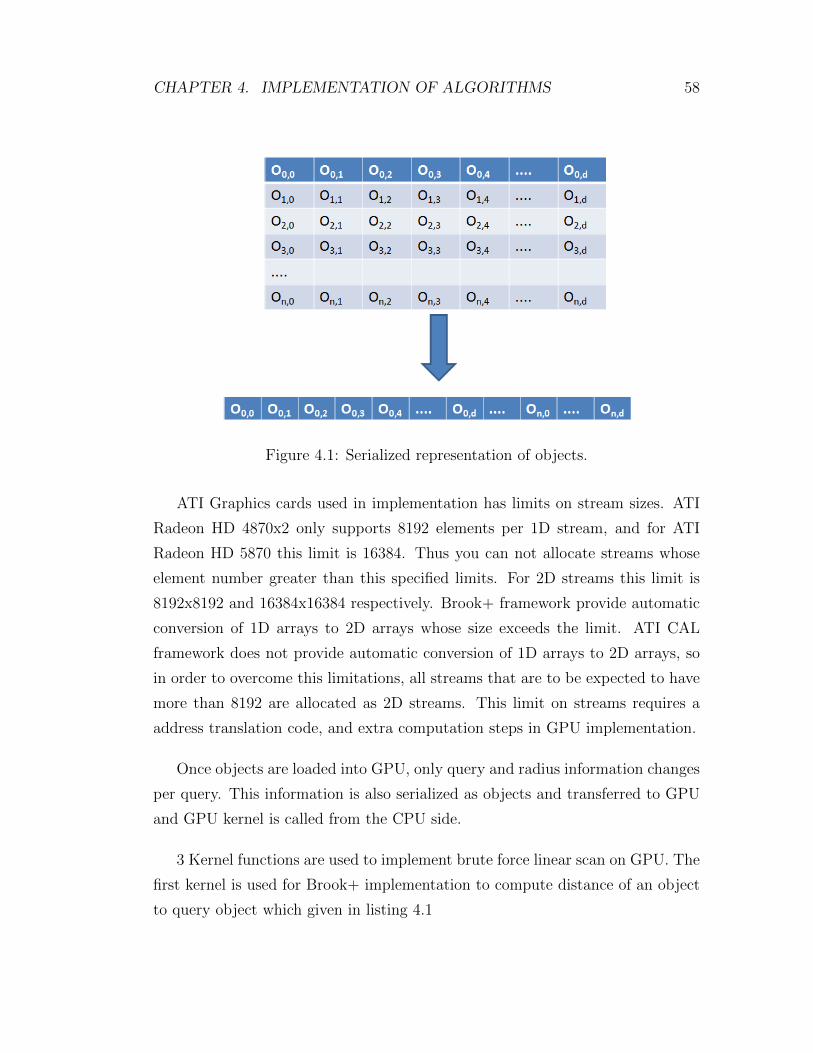
CHAPTER 4. IMPLEMENTATION OF ALGORITHMS 58
Figure 4.1: Serialized representation of objects.
ATI Graphics cards used in implementation has limits on stream sizes. ATI
Radeon HD 4870x2 only supports 8192 elements per 1D stream, and for ATI
Radeon HD 5870 this limit is 16384. Thus you can not allocate streams whose
element number greater than this specified limits. For 2D streams this limit is
8192x8192 and 16384x16384 respectively. Brook+ framework provide automatic
conversion of 1D arrays to 2D arrays whose size exceeds the limit. ATI CAL
framework does not provide automatic conversion of 1D arrays to 2D arrays, so
in order to overcome this limitations, all streams that are to be expected to have
more than 8192 are allocated as 2D streams. This limit on streams requires a
address translation code, and extra computation steps in GPU implementation.
Once objects are loaded into GPU, only query and radius information changes
per query. This information is also serialized as objects and transferred to GPU
and GPU kernel is called from the CPU side.
3 Kernel functions are used to implement brute force linear scan on GPU. The
first kernel is used for Brook+ implementation to compute distance of an object
to query object which given in listing 4.1

CHAPTER 4. IMPLEMENTATION OF ALGORITHMS 59
1 ke rne l f loat distL2D ( f l o a t 4 ob j e c t [ ] , int o f f s e t ,
2 f l o a t 4 queryObject [ ] , int d)
3 {4 int i = 0 ;
5 f l o a t 4 d i f f ;
6 f l o a t 4 t o t a l = f l o a t 4 ( 0 . 0 f , 0 . 0 f , 0 . 0 f , 0 . 0 f ) ;
7
8 for ( i =0; i<d ; i++){9 d i f f = ob j e c t [ o f f s e t+i ]−queryObject [ i ] ;
10 t o t a l += d i f f ∗ d i f f ;11 }12 return s q r t ( t o t a l . x+t o t a l . y+t o t a l .w+t o t a l . z ) ;
13 }
Listing 4.1: Brook+ Kernel for distance computation
This kernel is a reduce kernel which computes distance from query object to
a given object using euclidean distance. First parameter is a float4 stream rep-
resenting objects. Second parameter named offset, and represents the starting
index of object whose distance to query object is to be computed. Third param-
eter is query object stream and finally fourth parameter is the dimension of the
object divided by four.
distL2D kernel computes euclidean distance of query object to some given
object. Lines 4-5 initializes variables used in kernel. Local variable i used as loop
counter, diff to hold difference between each vector coordinate, total is used to
hold running cumulative sum of squared differences. Local variables are defined
as float4, which is basically a record of 4 floats. Advantage of this type is that
it enables use of packed arithmetic operations. Packed version of arithmetic
operations performs the operation simultaneously on the corresponding fields of
the record. Consider following code:

CHAPTER 4. IMPLEMENTATION OF ALGORITHMS 60
f loat val1x , val2x , rx ;
f loat val1y , val2y , ry ;
f loat val1w , val2w , rw ;
f loat val1z , val2z , rz ;
rx = val1x ∗ val2x ;
ry = val1y ∗ val2y ;
rw = val1w∗val2w ;
rz = va l1z ∗ va l2z ;
which is equivalent to following code
f l o a t 4 val1 , val2 , r ;
r = val1 ∗ va l2 ;
because of packed operation instructions available in GPU.
In each loop iteration difference between vector coordinates is computed,
squared and added to running sum total. As it can be seen loop does not run num-
ber of dimension times, as would expected. It runs number of dimensions/4 times
because of and architecture of GPU supports 4 operations in one instruction. As
depicted in figure 4.2, by using float4 type loop is optimized by performing 4
coordinate pair differences in one instruction.
Similarly running sum and squaring of difference in line 10, also benefits by
performing operations in one instruction. Instead of d * (1 subtraction+1 multi-
plication+1 addition), packed versions of operations are performed in GPU thus
number of required clock cycles is reduced by 4. Finally in line 12 each separate
running sum in float4 structure is summed and square root of total is returned
as distance.
Second kernel used in Brook+ implementation is given in listing 4.2

CHAPTER 4. IMPLEMENTATION OF ALGORITHMS 61
Figure 4.2: Packed instruction execution.
1 ke rne l void BROOK linear scan r query ( f l o a t 4 ob j e c t [ ] , int d , f l o a t 4
queryObject [ ] ,
2 out f loat di s tance<>)
3 {4 d i s t ance = distL2D ( object , i n s t ance ( ) . x∗d , queryObject , d ) ;
5 }
Listing 4.2: Brook+ Kernel for Brute Force Search
This kernel calls first kernel for each object in objects collection. Although
no for loop is present, code defined in the kernel is invoked per each output
stream element, which is named distance. First parameter of kernel is object
stream which holds objects whose distance is to be computed. Second parameter
is dimensions of objects /4 and third parameter is query object stream. In line
4 kernel invokes distL2D kernel by passing object and query streams, along with
dimension information. Index of object whose distance to query object is to
be computed is determined by instance() primitive of Brook+ language, which
returns index of output stream for which kernel is invoked.
ATI Cal implementation of Brute Force Search kernel is given in listing 4.3

CHAPTER 4. IMPLEMENTATION OF ALGORITHMS 62
1 ke rne l void CAL l inear scan r query ( int indexMetaData [ ] ,
2 f l o a t 4 ob j e c t [ ] [ ] , f l o a t 4 queryObject [ ] , out f loat di s tance<>)
3 {4 int i =0;
5 int width = indexMetaData [ 0 ] ;
6 int d = indexMetaData [ 2 ] ;
7 f l o a t 4 d i f f ;
8 f l o a t 4 t o t a l = f l o a t 4 ( 0 . 0 f , 0 . 0 f , 0 . 0 f , 0 . 0 f ) ;
9 in t2 idx = in s t ance ( ) . xy ;
10 int actua l Index = ( idx . y∗width+idx . x ) ;
11
12 i f ( actua l Index >= indexMetaData [ 1 ] ) {13 return ;
14 }15 actua l Index = actua l Index ∗ d ;
16
17 idx . x = actua l Index % width ;
18 idx . y = actua l Index / width ;
19
20
21 for ( i =0; i<d ; i++){22 d i f f = ob j e c t [ idx . y ] [ idx . x]−queryObject [ i ] ;
23 t o t a l += d i f f ∗ d i f f ;24 idx . x++;
25 i f ( idx . x >= width ) {26 idx . y ++;
27 idx . x = 0 ;
28 }29 }30 d i s t ance = sq r t ( t o t a l . x+t o t a l . y+t o t a l .w+t o t a l . z ) ;
31 }
Listing 4.3: ATI CAL Kernel for Brute Force Search
This kernel differs from Brook+ kernel as there is no automatic address trans-
lation support in ATI Cal framework, also distance computation kernel is un-
folded. First parameter of this kernel is indexMetaData, which consists of several
values guiding computation in kernel. First value in indexMetaData stream is

CHAPTER 4. IMPLEMENTATION OF ALGORITHMS 63
supposed to be the width of distance stream, hence object stream. Second value
is the number of objects in object collection and third value is the number of
dimensions/4.
Lines 4 to 10 consists of initialization of local variables used in kernel.
In line 12 a check is performed to terminate kernel if computations is not
necessary. This is because of the stream size limits imposed by graphic card. Since
we can not allocate arbitrary sized 1D streams, 2D stream is allocated if limit is
surpassed. Width of 2D stream is set to maximum allowed value and height is
computed accordingly. This approach can sometimes allocate unnecessary space,
if total number of objects is not multiple of maximum 2D stream width. Line 12
checks this condition and exits from kernel without any further computation.
Line 17 and 18 translates 1D index to 2D stream index and in for loop starting
on line 21 computes euclidean distance of object to query object in similar fashion
as in Brook+ kernel.
4.2 KVP Implementation GPU
KVP algorithm is chosen for implementation because it readily supports paral-
lelization.This structure is unique since it improves both the storage and compu-
tational overhead of the classical vantage-points approach. The KVP structure
offers a number of benefits:
1. It is a simple data structure and can be implemented relatively easily.
2. It can support dynamic operations like insertion and deletion.
3. It is easily adapted for use as a disk-based structure and its access patterns
minimize the number of disk-seek operations.
4. Queries may be executed in parallel.
CHAPTER 4. IMPLEMENTATION OF ALGORITHMS 64
KVP algorithm utilizes precomputed object to pivot distances to reduce num-
ber of distance computations in a similarity search. Given a query, algorithm first
computes distances to pivots from query object. These distances, along with pre-
computed object to pivot distances are used to set a bound on query to object
distances. If distance bounds are found to be greater than search radius query
object is discarded. If upper bound for distance is smaller than radius, then
object is added to result set without any need for actual distance computation.
The first step of GPU adaptation of the algorithm is to load object collection
into graphic card texture memory as in brute force search method. This step is
performed similar to GPU adaptation of Brute Force search.
Second step is to load index structure into memory. The same limitations
on streams sizes and memory copy requirements apply, so KVP representation is
modified to adapt GPU. Original implementation of KVP stores a record per ob-
ject which consist of object pivot distances and indexes to pivots whose distances
is precomputed. In our implementation, they are represented as a single array
of object to pivots distances and pivot indexes respectively. This representation
enables loading of KVP structure into graphic card memory without temporary
memory copy operations.
Another modification to original implementation was to change data struc-
ture which hold the indexes of pivots used in KVP. Since GPU adaptation of
KVP designed to utilize all graphic processing units available on a system, this
representation posed a problem. When there is more than one graphic processor
present in the system processing of query is divided between each graphic process-
ing unit by assigning a part of object collection to each graphic processing unit.
Thus not every object is present in each graphical processing unit, and indexes to
pivots are not useful. So instead of passing indexes of pivots in collection, pivot
object is passed instead.
Once objects are loaded into GPU, only query and radius information changes
per query. This information is also serialized as objects and transferred to GPU
and GPU kernel is called from the CPU side.

CHAPTER 4. IMPLEMENTATION OF ALGORITHMS 65
5 Kernel functions are used to implement brute KVP algorithm on GPU. The
first kernel is used for address translation of indexes for objects. As noted before
this was due to stream size limitations of graphics cards. Kernel listed in listing
4.4 takes two arguments, actual index of object in 1D streams and maximum 2D
width allowed by graphic card. Using this values objects index is calculated and
result is returned in structure consisting of two integers.
1 ke rne l i n t2 t rans l a t eAddre s s ( int actual Index , int width )
2 {3 in t2 idx ;
4 idx . x = actua l Index % width ;
5 idx . y = actua l Index / width ;
6 return idx ;
7 }
Listing 4.4: ATI CAL kernel for Address Translation
Next kernel is implemented to perform distance computations between query
object and a object whose index is given. Listing for this kernel is show in listing
4.5.

CHAPTER 4. IMPLEMENTATION OF ALGORITHMS 66
1 ke rne l f loat distL2D ( f l o a t 4 ob j e c t [ ] [ ] , int d , f l o a t 4 queryObject [ ] ,
int l o g i c a l I ndex , int width )
2 {3 int i =0;
4 f l o a t 4 d i f f ;
5 f l o a t 4 t o t a l = f l o a t 4 ( 0 . 0 f , 0 . 0 f , 0 . 0 f , 0 . 0 f ) ;
6
7 in t2 idx = trans l a t eAddre s s ( l o g i c a l I nd e x ∗d , width ) ;
8
9 for ( i =0; i<d ; i++){10 d i f f = ob j e c t [ idx . y ] [ idx . x]−queryObject [ i ] ;
11 t o t a l += d i f f ∗ d i f f ;12 idx . x++;
13 i f ( idx . x >= width ) {14 idx . y ++;
15 idx . x = 0 ;
16 }17 }18 return s q r t ( t o t a l . x+t o t a l . y+t o t a l .w+t o t a l . z ) ;
19 }
Listing 4.5: ATI CAL kernel for Object distance computation
distL2D kernel after local variable initialization, actual index of object whose
distance is to be computed is found. Then euclidean distance computation is
performed similar to Brute Force Search.
The kernel presented on listing 4.6 used for computing distance from query
object to each pivot in KVP structure. It consists of one line, a call to distL2D
kernel with appropriate parameters. After execution of this kernel queryPivot-
Distance stream contains distance of query to each pivot, which is later used on
computation of object to query distance bounds.

CHAPTER 4. IMPLEMENTATION OF ALGORITHMS 67
1 ke rne l void computeQueryToPivotDistances ( int indexMetaData [ ] , f l o a t 4
ob j e c t [ ] [ ] , f l o a t 4 queryObject [ ] , out f loat queryPivotDistance<>)
2 {3 queryPivotDistance = distL2D ( object , indexMetaData [ 2 ] , queryObject ,
i n s t anc e ( ) . x , indexMetaData [ 0 ] ) ;
4 }
Listing 4.6: ATI CAL kernel for Query object to pivot distance computation
Kernel computeDistanceBounds which is show in listing 4.7, computes dis-
tance bounds for an object whose index is specified. First argument of kernel,
indexMetaData stream, is used to pass index and graphic card specific informa-
tion to kernel. First value of stream contains maximum 2D width supported by
graphic card. Second value is the number of objects in object collection. Third
value is dimensions of objects divided by four, as objects are represented as float4
streams. Lastly fourth value is the number of pivots selected during KVP index
construction. Next parameter of the kernel is a stream used to represent ob-
ject pivot distances. Third parameter is a stream representing indexes of pivots
whose distance to objects is precomputed. Fourth parameter is the query to pivot
distances. Last two parameters are query radius and index of the object whose
distance bounds is to be computed.
After initialization in computeDistanceBounds kernel, for loop in line 10
computes minimum and maximum possible distance of object to query ob-
ject using precomputed object to pivot distance. In each iteration of loop,
a pivot next in sequence of pivots is selected (Line 11). According triangle
inequality of metric spaces, upper bound for this objects distance should be
d(query,pivot)+d(pivot,object). If this maximum possible distance is greater than
query radius, which implies that object is query result set, this maximum distance
value is returned without considering other pivots. If it is not smaller or equal to
query radius than minimum possible distance is computed. Again this minimum
on distance value is checked against query radius. If minimum possible distance
value is greater than query radius, which implies that object is not definitely in
query result set, minimum distance is returned without considering remaining
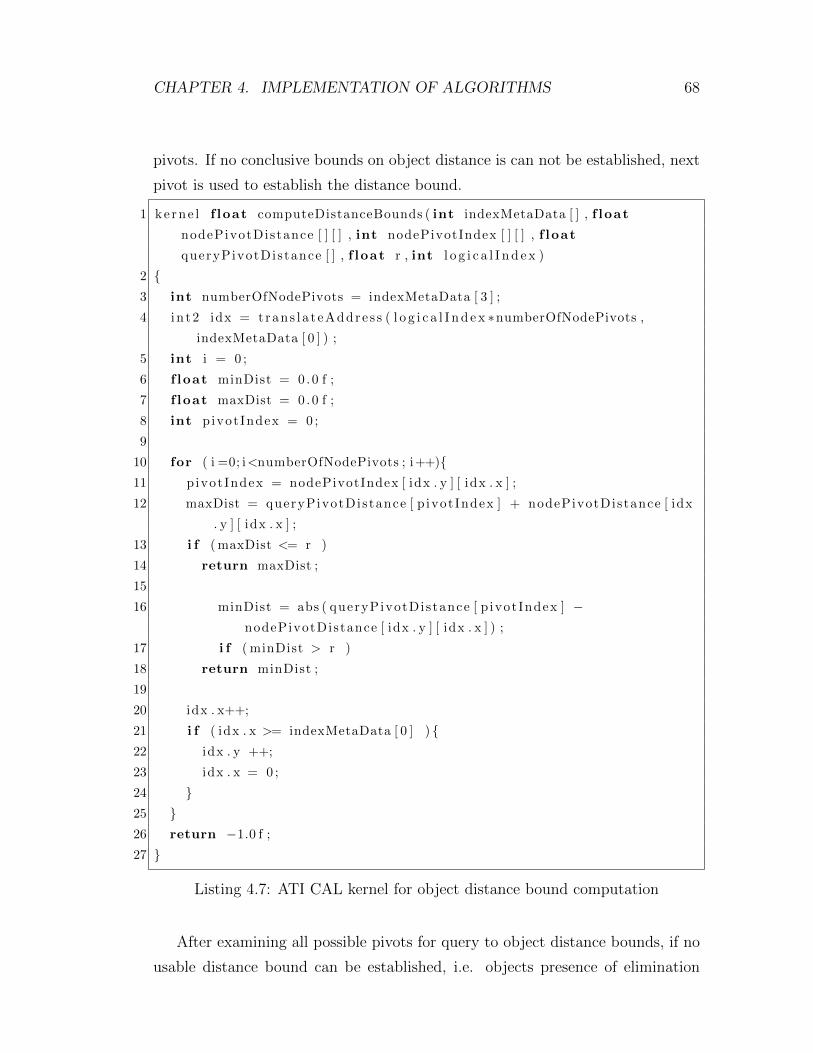
CHAPTER 4. IMPLEMENTATION OF ALGORITHMS 68
pivots. If no conclusive bounds on object distance is can not be established, next
pivot is used to establish the distance bound.
1 ke rne l f loat computeDistanceBounds ( int indexMetaData [ ] , f loat
nodePivotDistance [ ] [ ] , int nodePivotIndex [ ] [ ] , f loat
queryPivotDistance [ ] , f loat r , int l o g i c a l I nd e x )
2 {3 int numberOfNodePivots = indexMetaData [ 3 ] ;
4 i n t2 idx = trans l a t eAddre s s ( l o g i c a l I nd e x ∗numberOfNodePivots ,
indexMetaData [ 0 ] ) ;
5 int i = 0 ;
6 f loat minDist = 0 .0 f ;
7 f loat maxDist = 0 .0 f ;
8 int pivotIndex = 0 ;
9
10 for ( i =0; i<numberOfNodePivots ; i++){11 pivotIndex = nodePivotIndex [ idx . y ] [ idx . x ] ;
12 maxDist = queryPivotDistance [ p ivot Index ] + nodePivotDistance [ idx
. y ] [ idx . x ] ;
13 i f (maxDist <= r )
14 return maxDist ;
15
16 minDist = abs ( queryPivotDistance [ p ivotIndex ] −nodePivotDistance [ idx . y ] [ idx . x ] ) ;
17 i f ( minDist > r )
18 return minDist ;
19
20 idx . x++;
21 i f ( idx . x >= indexMetaData [ 0 ] ) {22 idx . y ++;
23 idx . x = 0 ;
24 }25 }26 return −1.0 f ;27 }
Listing 4.7: ATI CAL kernel for object distance bound computation
After examining all possible pivots for query to object distance bounds, if no
usable distance bound can be established, i.e. objects presence of elimination

CHAPTER 4. IMPLEMENTATION OF ALGORITHMS 69
from query result set can be proved, object is marked for distance computation
by returning special value -1.
Last kernel implementation for KVP algorithm is presented in listing 4.8. This
kernel starts computation by checking whether this invocation is for a valid object.
If it is not it immediately returns. If it is for a valid object, first distance bounds
on object is computed. If result of distance bound computation is conclusive so
as to decide whether include object in result set or eliminate it kernel returns. If
not distance from query to object is computed (Line 11).
1 ke rne l void computeObjectQueryDistances ( int indexMetaData [ ] , f l o a t 4
ob j e c t [ ] [ ] , f loat nodePivotDistance [ ] [ ] , int nodePivotIndex [ ] [ ] ,
f loat queryPivotDistance [ ] , f loat r , f l o a t 4 queryObject [ ] , out f loat
di s tance<>)
2 {3 in t4 index = in s t ance ( ) ;
4 int ob jec t Index = index . y∗ indexMetaData [0 ]+ index . x ;
5 f loat d i s t ;
6
7 i f ( ob jec t Index >= indexMetaData [ 1 ] )
8 return ;
9 d i s t = computeDistanceBounds ( indexMetaData , nodePivotDistance ,
nodePivotIndex , queryPivotDistance , r , ob j ec t Index ) ;
10 i f ( d i s t == −1.0 f )11 d i s t = distL2D ( object , indexMetaData [ 2 ] , queryObject , object Index ,
indexMetaData [ 0 ] ) ;
12 d i s t ance = d i s t ;
13 }
Listing 4.8: ATI CAL kernel for KVP algorithm
4.3 Filtering Results on GPU
Adaptations of search algorithms presented in this thesis rely on the fragment
processor, which operates across a large set of output memory locations, consum-
ing a fixed number of input elements per location and operating a small program

CHAPTER 4. IMPLEMENTATION OF ALGORITHMS 70
on those elements to produce a single output element in that location. Because
the fragment program must write its results to a preordained memory location,
it is not able to vary the amount of data that it outputs according to the input
data it processes.
Many algorithms are difficult to implement under these limitations, specif-
ically, algorithms that reduce many data elements to few data elements. The
reduction of data by a fixed factor has been carefully studied on GPUs [12]; such
operations require an amount of time linear in the size of the data to be reduced.
However, nonuniform reductionsthat is, reductions that filter out data based on
its content on a per element basis have been less thoroughly studied, yet they are
required for a number of interesting applications.
Search algorithms presented in this thesis does not specifically require distance
filtering to be performed on GPU. Filtering of results, i.e. deciding whether an
object is in result set based on its distance which is basically a condition check on
an array of distance values, can be performed in CPU side. Even filtering result
set on CPU provides speed up of several times in execution times, as bulk of
the time is spent on distance computations. Thus and implementation provided
still benefit acceleration by utilization of graphic cards, yet if this filtering can be
performed efficiently in GPU, additional speed up can be obtained by eliminating
some data transfer from GPU to CPU. In order to explore this possibility a result
set filtering algorithm that makes it possible to perform filtering GPU is presented
is also designed.
Our problem is to eliminate objects from result set that have distance value
greater than specified query radius. Several approaches can be used. The most
obvious method for compaction can be a stable sort to eliminate the records;
however, using bitonic sort to do this will result in a running time of O(n (log
n)2) ([13]). Instead, we present a technique here that uses a scan ([37]) to obtain
a running count of the number of distances that are smaller or equal to query
radius, and then use a scatter pass to compact them, for a final running time of
O(n log n) similar the algorithm given [72] .
Given a list of objects, to decide where a particular object redirect itself, it

CHAPTER 4. IMPLEMENTATION OF ALGORITHMS 71
is sufficient to count the number of distances that are smaller or equal to query
radius to the left of the each distance, then move the object that many records
to the left. On a parallel system, the cost of finding a running count is actually
O(n log n). The multipass technique to perform a running sum is called a scan.
It starts by counting the number of valid distance in the current record. This
number is saved to a stream for further processing. The kernel for this part is
listed in listing 4.9
1 ke rne l void i n i t i a l i z e r e s u l t s i n d e x ( f loat di s tance <>, f loat rad iu s ,
out int r e s u l t s i nd ex <>,out int r e s u l t s i nd ex2 <>)
2 {3 i f ( d i s t anc e > rad iu s ) {4 r e s u l t s i n d e x = 0 ;
5 r e s u l t s i n d e x 2 = 0 ;
6 }7 else {8 r e s u l t s i n d e x = 1 ;
9 r e s u l t s i n d e x 2 = 1 ;
10 }11 }
Listing 4.9: ATI CAL Kernel for Result Set Filtering Initialization
Now each record in the stream holds the number of valid distances (distances
thats are smaller or equal to query radius) at its location, which is 0 or 1. This
can be used to the algorithm’s advantage in another pass, where the stream sums
itself with records indexed to the left and saves the result to a new stream. Now
each record in the new stream effectively has added the number of valid distances
at its current position and left of it. The subsequent steps add their values to
values indexed at records of increasing powers of two to their left, until the power
of two exceeds the length of the input array. This process is illustrated in Figure
4.3.
Kernel used for this multipass operation is presented in listing 4.10

CHAPTER 4. IMPLEMENTATION OF ALGORITHMS 72
Figure 4.3: Iteratively counting number of objects in result set.
1 ke rne l void s can index ( int metaData [ ] , int twotoi , int input [ ] [ ] , out
int r e s u l t s i nd ex <>)
2 {3 in t2 c index = in s t ance ( ) . xy ;
4 int l o g i c a l I nd e x = (metaData [ 0 ] ∗ c index . y )+cindex . x−twoto i ;
5 int va l = input [ c index . y ] [ c index . x ] ;
6
7 i f ( l o g i c a l I nd e x >= metaData [ 1 ] )
8 return ;
9
10 i f ( l o g i c a l I nd e x >= 0) {11 c index . x = l o g i c a l I n d e x % metaData [ 0 ] ;
12 c index . y = l o g i c a l I n d e x / metaData [ 0 ] ;
13 va l += input [ c index . y ] [ c index . x ] ;
14 }15 r e s u l t s i n d e x = va l ;
16 }
Listing 4.10: ATI CAL Kernel for Result Set Filtering Scan

CHAPTER 4. IMPLEMENTATION OF ALGORITHMS 73
After performing this multipass counting kernel log n times, each record knows
how many valid distances are present before them. The value at the very right of
the stream indicates how many objects there are in the result set, and hence the
length of the compacted output. To get size of result set kernel listed in listing
4.11 is invoked.
1 ke rne l void r e s u l t s e t s i z e ( int metaData [ ] , int r e s u l t s i n d e x [ ] [ ] , out
int count<>)
2 {3 in t2 index ;
4 index . x = (metaData [1 ]−1) % metaData [ 0 ] ;
5 index . y = (metaData [1 ]−1) / metaData [ 0 ] ;
6 count = r e s u l t s i n d e x [ index . y ] [ index . x ] ;
7 }
Listing 4.11: ATI CAL Kernel for Obtaining Result Set Size
If result set size greater than zero, a new stream where first number of result
set size elements contains indexes of objects that are in result set is computed
through a scatter operation. As in this step each value in the stream holds number
of valid distances to left of it (counting it self also), its position on this new stream
is its value minus one. Kernel implementing scatter operation is listed in listing
4.12
1 ke rne l void f i l t e r r e s u l t s ( int metaData [ ] , f loat radius , f loat
di s tance <>,int r e s u l t s i nd ex <>,out int f i l t e r e d i n d e x [ ] [ ] )
2 {3 in t2 index = in s t ance ( ) . xy ;
4 int i n pu t l o g i c a l I nd ex ;
5 int ou tpu t l og i c a l I ndex ;
6 i f ( rad iu s >= di s t ance ) {7 i npu t l o g i c a l I nd ex = (metaData [ 0 ] ∗ index . y )+index . x ;
8
9 i f ( i npu t l o g i c a l I nd ex >= metaData [ 1 ] )
10 return ;
11
12 ou tpu t l og i c a l I ndex = r e s u l t s i nd ex −1;13 index . x = outpu t l og i c a l I ndex % metaData [ 0 ] ;
14 index . y = outpu t l og i c a l I ndex / metaData [ 0 ] ;

CHAPTER 4. IMPLEMENTATION OF ALGORITHMS 74
15
16 f i l t e r e d i n d e x [ index . y ] [ index . x ] = inpu t l o g i c a l I nd ex ;
17 }18 }
Listing 4.12: ATI CAL Kernel for Filtering Result set
Now we have a stream which contain indexes of objects which are in the result
set, a new stream with appropriate size is created to retrieve index and computed
distance to query object. Kernel listed in listing 4.13 is used to copy results back
to system memory.
1 ke rne l void c o p y f i l t e r e d r e s u l t s ( int metaData [ ] , f loat d i s t anc e [ ] [ ] ,
int r e s u l t s i n d e x [ ] [ ] , out f l o a t 2 r e s u l t s e t <>)
2 {3 f l o a t 2 va l ;
4
5 int c index = ( ( in s t anc e ( ) . y∗metaData [ 0 ] )+in s tance ( ) . x ) ∗4 ;6 int r index = r e s u l t s i n d e x [ c index /metaData [ 0 ] ] [ c index % metaData
[ 0 ] ] ;
7 int x = r index % metaData [ 0 ] ;
8 int y = r index / metaData [ 0 ] ;
9 va l . x = ( f loat ) r index ;
10 va l . y = d i s t ance [ y ] [ x ] ;
11 r e s u l t s e t = va l ;
12 }
Listing 4.13: ATI CAL Kernel for copying Filtered Result set

Chapter 5
Experiment Results
Experimental data are collected using a system which had 2 graphics cards; ATI
Radeon 4870x2 (2GB) and ATI Radeon 5870 (1GB), 6GB of system memory with
Intel i7 cpu. Details of system configuration is given in table 5.1 Implementation
is done on C++ and compiled with all optimization flags enabled. In order to
utilize all the multi-threading capabilities of cpu, cpu versions of algorithms are
run in 8 (which produced the best performance) different threads. In these tests,
measurements are performed by following steps:
1. Initialization: objects,index structures and queries are loaded.
2. Warming Run: before measuring execution time, a warming run for the
query is performed.
3. Query Execution: 1000 queries are repeatedly executed to minimize mea-
surement errors and elapsed time is reported.
The synthetic data used in these tests consists of randomly generated vectors
with varying dimensions (16,32,48,64,80,96,112,128,144 and 160). Each dimen-
sion is random coordinate value uniformly distributed over the range [0.0− 1.0].
The object collection on which similarity queries were executed consisted of 220
vectors up to 10×220 vectors. Measurements of timings are grouped into two test
75

CHAPTER 5. EXPERIMENT RESULTS 76
Test Hardware
Processor Intel Core i7-920 (Bloomfield) 2.66 GHz, 8 MB L3 Cache,power-saving settings disabled
Motherboard LANPARTY DK X58-T3eH6Memory Corsair Dominator 6GB (3 x 2GB) DDR3-1600 8-8-8-24 @
1,600 MHzGraphics Cards ATI Radeon HD 4870x2
ATI Radeon HD 5870
System Software and Drivers
Operating System Microsoft Windows 7 Ultimate x64Graphics Driver AMD Catalyst 9.12
Table 5.1: System configuration of Test Hardware
Test Set 1 Test Set 2Run# Dimension Object Count Dimension Object Count1 16 1048576 16 10485762 32 1048576 16 20971523 48 1048576 16 31457284 64 1048576 16 41943045 80 1048576 16 52428806 96 1048576 16 62914567 112 1048576 16 73400328 128 1048576 16 83886089 144 1048576 16 943718410 160 1048576 16 10485760
Table 5.2: Number of objects and dimension sizes used in measurements.
sets and named as test set 1 and test set 2. Test set 1 aims to measure effect of
dimensionality on execution times, by taking execution times with same object
count (220) and varying dimensions. Test set 2 aims to measure effect of object
count on execution times, by taking execution times with same dimensionality
(16) and varying object count. Table 5.2 shows object counts and dimension sizes
used in each test set
Only results of ATI CAL implementation is reported in this work, as Brook+
and OpenCL implementation performances were similar, as they are built on ATI
CAL framework in implementations provided by ATI.

CHAPTER 5. EXPERIMENT RESULTS 77
These test sets are measured against various implementations. First GPU
implementations where distance computations were done in GPU, distance val-
ues returned to system memory and result set filtering was done on CPU were
measured. Then in order to see effect of GPU to CPU data transfers, same tests
are repeated and execution times are measured for the modified implementation
where there were no distance value transfer from GPU to system memory. Lastly
same tests are repeated with implementation where filtering performed on GPU
and only result set is transferred from GPU to system memory.
In the following sub-sections we report results of theses experiments.
5.1 Comparison of implementations with Result
Set Filtering on CPU
In these tests, aim was to measure speedups obtained by GPU utilization in dis-
tance computation. Implementations used in this test compute distance values
on the GPU and reports back query to object distance for each object. Dis-
tance function was selected to be euclidean distance of query and object vectors.
Filtering of distances are done on CPU side.
D N Linear Scan KVP CAL KVP CAL16 1048576 59.11 35.25 20.16 22.1832 1048576 101.13 36.87 21.19 21.9448 1048576 140.81 37.18 22.18 21.9964 1048576 182.76 30.53 22.67 21.9280 1048576 223.68 32.25 23.95 22.0696 1048576 264.41 36.11 25.09 22.13112 1048576 301.96 35.95 27.31 19.54128 1048576 355.24 37.84 27.99 20.86144 1048576 385.97 38.17 30.78 20.45160 1048576 427.46 39.66 30.81 20.03
Table 5.3: Execution times in seconds for 1000 radius queries on object set sizeof 220 vectors, with varying vector dimensions. Result set filtering performed onCPU.

CHAPTER 5. EXPERIMENT RESULTS 78
In order to see effects of object dimension size and object collection size two
sets of different tests were performed. In test set 1, dimension of the vectors
were changed between 16 to 160, by increments of 16, and number of objects are
kept constant at 220. Table 5.3 shows measured timings for test set 1, figure 5.1
shows results as chart. Figure 5.2 shows speed up factors for each implementation
compared to CPU brute force search.
Figure 5.1: Execution times in seconds for 1000 radius queries on 220 vectors,with varying vector dimensions. Result set filtering performed on CPU.
Figure 5.2: Relative speeds of implementations for test set 1, when result setfiltering is performed on CPU.
Results show that as the number of dimensions increase, GPU versions of
the algorithms perform considerable better from CPU versions. While in lower
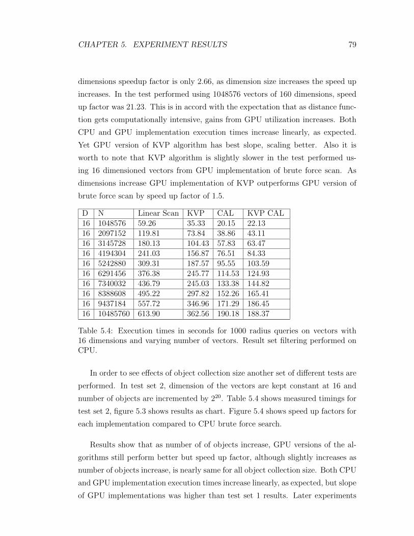
CHAPTER 5. EXPERIMENT RESULTS 79
dimensions speedup factor is only 2.66, as dimension size increases the speed up
increases. In the test performed using 1048576 vectors of 160 dimensions, speed
up factor was 21.23. This is in accord with the expectation that as distance func-
tion gets computationally intensive, gains from GPU utilization increases. Both
CPU and GPU implementation execution times increase linearly, as expected.
Yet GPU version of KVP algorithm has best slope, scaling better. Also it is
worth to note that KVP algorithm is slightly slower in the test performed us-
ing 16 dimensioned vectors from GPU implementation of brute force scan. As
dimensions increase GPU implementation of KVP outperforms GPU version of
brute force scan by speed up factor of 1.5.
D N Linear Scan KVP CAL KVP CAL16 1048576 59.26 35.33 20.15 22.1316 2097152 119.81 73.84 38.86 43.1116 3145728 180.13 104.43 57.83 63.4716 4194304 241.03 156.87 76.51 84.3316 5242880 309.31 187.57 95.55 103.5916 6291456 376.38 245.77 114.53 124.9316 7340032 436.79 245.03 133.38 144.8216 8388608 495.22 297.82 152.26 165.4116 9437184 557.72 346.96 171.29 186.4516 10485760 613.90 362.56 190.18 188.37
Table 5.4: Execution times in seconds for 1000 radius queries on vectors with16 dimensions and varying number of vectors. Result set filtering performed onCPU.
In order to see effects of object collection size another set of different tests are
performed. In test set 2, dimension of the vectors are kept constant at 16 and
number of objects are incremented by 220. Table 5.4 shows measured timings for
test set 2, figure 5.3 shows results as chart. Figure 5.4 shows speed up factors for
each implementation compared to CPU brute force search.
Results show that as number of of objects increase, GPU versions of the al-
gorithms still perform better but speed up factor, although slightly increases as
number of objects increase, is nearly same for all object collection size. Both CPU
and GPU implementation execution times increase linearly, as expected, but slope
of GPU implementations was higher than test set 1 results. Later experiments
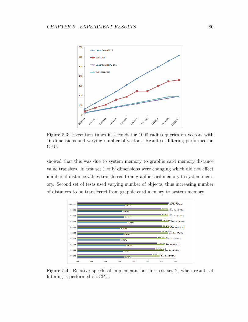
CHAPTER 5. EXPERIMENT RESULTS 80
Figure 5.3: Execution times in seconds for 1000 radius queries on vectors with16 dimensions and varying number of vectors. Result set filtering performed onCPU.
showed that this was due to system memory to graphic card memory distance
value transfers. In test set 1 only dimensions were changing which did not effect
number of distance values transferred from graphic card memory to system mem-
ory. Second set of tests used varying number of objects, thus increasing number
of distances to be transferred from graphic card memory to system memory.
Figure 5.4: Relative speeds of implementations for test set 2, when result setfiltering is performed on CPU.

CHAPTER 5. EXPERIMENT RESULTS 81
5.2 Performance Overhead of Data Transfers
from GPU to CPU
As it can be seen results of previous tests, memory transfers from GPU to CPU
has quite impact on execution times. The tests reported in this section are
performed to see how great this impact was.
D N Linear Scan KVP CAL KVP CAL16 1048576 59.11 35.25 2.17 2.5432 1048576 101.13 36.87 3.81 2.7048 1048576 140.81 37.18 5.21 2.8764 1048576 182.76 30.53 6.76 2.9080 1048576 223.68 32.25 8.23 3.0696 1048576 264.41 36.11 9.41 3.21112 1048576 301.96 35.95 11.27 3.20128 1048576 355.24 37.84 12.54 3.28144 1048576 385.97 38.17 14.09 3.35160 1048576 427.46 39.66 14.78 3.60
Table 5.5: Execution times in seconds for 1000 radius queries on object set sizeof 220 vectors, with varying vector dimensions, no result set fetching.
In order to measure effect of memory transfers from GPU to CPU, implemen-
tations were modified so as leave distances values on the graphic card memory.
Other than distance value fetch code from graphic memory, everything in the
code left same, which assures that GPU still computes the distance values. After
this modification same sets of tests performed. Table 5.5 shows measured timings
for test set 1, figure 5.5 shows results as chart. Figure 5.6 shows speed up factors
for each implementation compared to CPU brute force search.

CHAPTER 5. EXPERIMENT RESULTS 82
Figure 5.5: Execution times in seconds for 1000 radius queries on object set sizeof 220 vectors, with varying vector dimensions, no result set fetching.
Figure 5.6: Relative speeds of implementations for test set 1, no result set fetch-ing.

CHAPTER 5. EXPERIMENT RESULTS 83
When we compare these measurement of execution times with the implemen-
tations that fetch distance values from GPU memory, we can compute memory
transfer overheads from GPU to system memory. By dividing size of data trans-
ferred to time difference data transfer rate is calculated. Data transfer rates is
shown in Table 5.6.
D N Data (MB) Time(sec.) Transfer Rate (MB/sec) % Execu-tion
16 1048576 4,000 17.99 222.3213 89.25%32 1048576 4,000 17.39 230.0770 82.03%48 1048576 4,000 16.96 235.8018 76.49%64 1048576 4,000 15.91 251.4362 70.18%80 1048576 4,000 15.72 254.5087 65.62%96 1048576 4,000 15.68 255.1284 62.50%112 1048576 4,000 16.03 249.5135 58.71%128 1048576 4,000 15.45 258.8953 55.20%144 1048576 4,000 16.69 239.6985 54.22%160 1048576 4,000 16.03 249.4988 52.04%
16 1048576 4,000 18.00 222.2045 89.32%16 2097152 8,000 35.61 224.6259 91.64%16 3145728 12,000 53.48 224.3881 92.48%16 4194304 16,000 71.05 225.2083 92.86%16 5242880 20,000 89.02 224.6768 93.16%16 6291456 24,000 106.92 224.4599 93.36%16 7340032 28,000 124.67 224.5862 93.47%16 8388608 32,000 142.46 224.6204 93.56%16 9437184 36,000 160.41 224.4290 93.65%16 10485760 40,000 178.19 224.4748 93.70%
Table 5.6: Data Transfer rate and percentage of time used in data transfers.
Analysis of data shows data transfer rates are below theoretical value. Ac-
cording to PCI Express Base 2.0 specification on 15 January 2007 the per-lane
throughput is 500 MB/s. This means a 16-lane PCI connector which is supported
by graphic cards, can support throughput up to 8 GB/s aggregate. Observed max-
imum transfer rate was only 259MB/sec, which is far below theoretical value. In
order to understand reason for slow data transfers, transfer rate is measured
with a utility program provided by ATI, in order to identify non compliant or
fault motherboard or some other hardware issue. Measuring with utility program
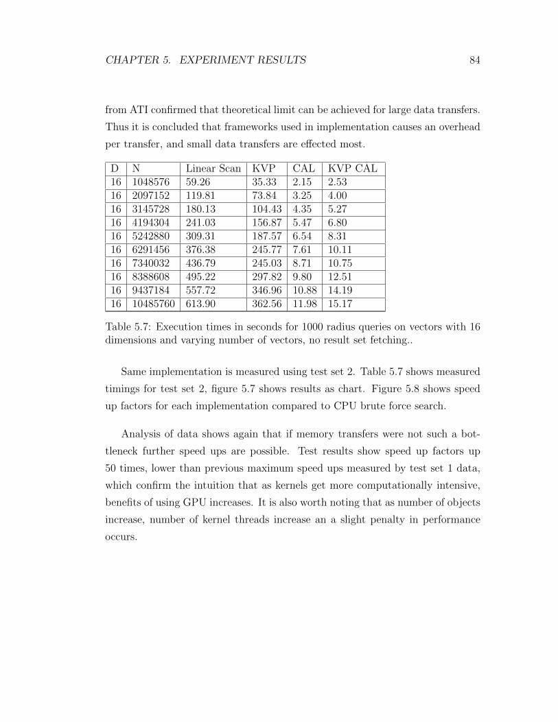
CHAPTER 5. EXPERIMENT RESULTS 84
from ATI confirmed that theoretical limit can be achieved for large data transfers.
Thus it is concluded that frameworks used in implementation causes an overhead
per transfer, and small data transfers are effected most.
D N Linear Scan KVP CAL KVP CAL16 1048576 59.26 35.33 2.15 2.5316 2097152 119.81 73.84 3.25 4.0016 3145728 180.13 104.43 4.35 5.2716 4194304 241.03 156.87 5.47 6.8016 5242880 309.31 187.57 6.54 8.3116 6291456 376.38 245.77 7.61 10.1116 7340032 436.79 245.03 8.71 10.7516 8388608 495.22 297.82 9.80 12.5116 9437184 557.72 346.96 10.88 14.1916 10485760 613.90 362.56 11.98 15.17
Table 5.7: Execution times in seconds for 1000 radius queries on vectors with 16dimensions and varying number of vectors, no result set fetching..
Same implementation is measured using test set 2. Table 5.7 shows measured
timings for test set 2, figure 5.7 shows results as chart. Figure 5.8 shows speed
up factors for each implementation compared to CPU brute force search.
Analysis of data shows again that if memory transfers were not such a bot-
tleneck further speed ups are possible. Test results show speed up factors up
50 times, lower than previous maximum speed ups measured by test set 1 data,
which confirm the intuition that as kernels get more computationally intensive,
benefits of using GPU increases. It is also worth noting that as number of objects
increase, number of kernel threads increase an a slight penalty in performance
occurs.

CHAPTER 5. EXPERIMENT RESULTS 85
Figure 5.7: Execution times in seconds for 1000 radius queries on vectors with 16dimensions and varying number of vectors, no result set fetching..
Figure 5.8: Relative speeds of implementations for test set 2, no result set fetch-ing.

CHAPTER 5. EXPERIMENT RESULTS 86
5.3 Comparison of implementations with Result
Set Filtering on GPU
If we look at table 5.6, we see that nearly %90 time is used for data transfers. So
it is expected that further acceleration is possible if this situation was remedied.
Since we had no control over frameworks used and PCI bus hardware, we tried to
reduce data size transferred. By performing filtering of distance values that are
greater than query radius on GPU side, we were able to reduce data transferred
at the expense of more computationally expensive filtering.
D N Linear Scan KVP CAL KVP CAL16 1048576 59.11 35.25 13.55 14.0132 1048576 101.13 36.87 14.94 14.1048 1048576 140.81 37.18 16.26 14.1064 1048576 182.76 30.53 16.82 14.1280 1048576 223.68 32.25 18.16 14.1696 1048576 264.41 36.11 19.15 14.53112 1048576 301.96 35.95 21.32 14.49128 1048576 355.24 37.84 22.03 14.44144 1048576 385.97 38.17 24.10 15.71160 1048576 427.46 39.66 24.72 16.02
Table 5.8: Execution times in seconds for 1000 radius queries on object set sizeof 220 vectors, with varying vector dimensions, GPU result set filtering.
D N Linear Scan KVP CAL KVP CAL16 1048576 59.26 35.33 13.49 13.9116 2097152 119.81 73.84 19.28 20.1616 3145728 180.13 104.43 28.21 29.3116 4194304 241.03 156.87 35.37 37.3816 5242880 309.31 187.57 47.33 49.6716 6291456 376.38 245.77 56.45 59.6716 7340032 436.79 245.03 62.59 65.2816 8388608 495.22 297.82 71.41 74.7016 9437184 557.72 346.96 82.97 87.2516 10485760 613.90 362.56 92.07 96.10
Table 5.9: Execution times in seconds for 1000 radius queries on vectors with 16dimensions and varying number of vectors, GPU result set filtering.
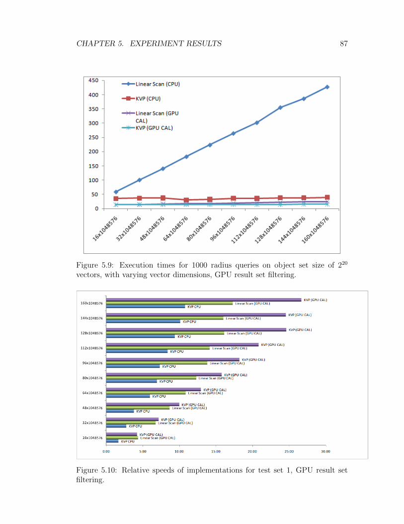
CHAPTER 5. EXPERIMENT RESULTS 87
Figure 5.9: Execution times for 1000 radius queries on object set size of 220
vectors, with varying vector dimensions, GPU result set filtering.
Figure 5.10: Relative speeds of implementations for test set 1, GPU result setfiltering.

CHAPTER 5. EXPERIMENT RESULTS 88
Figure 5.11: Execution times for 1000 radius queries on vectors with 16 dimen-sions and varying number of vectors, GPU result set filtering.
Figure 5.12: Relative speeds of implementations for test set 2, GPU result setfiltering.
Same sets of tests are performed and results are presented in Table 5.8 which
shows measured timings for test set 1, figure 5.9 shows results as chart. Figure
5.10 shows speed up factors for each implementation compared to CPU brute
force search. Table 5.9 shows measured timings for test set 2, figure 5.11 shows
results as chart. Figure 5.12 shows speed up factors for each implementation
compared to CPU brute force search.
Results show that as number of dimensions increase, GPU versions of the
algorithms perform considerable better from CPU versions in accordance with

CHAPTER 5. EXPERIMENT RESULTS 89
previous tests. While in lower dimensions speedup factor is only 4.36, as dimen-
sion size increases speed up increases. In tests performed using 1048576 vectors
of 160 dimensions, speed up factor was 26.68. This was an improvement over
implementing filtering in CPU, which yielded speed up factor of 21.23.

Chapter 6
Conclusion
The field of GPGPU computing is advancing quickly. Many GPGPU algorithms
continue to be developed for a wide range of problems, from physical simulations
to data mining. Current graphics APIs, and GPGPU languages, provide a fast
computation platform, hiding much of the complexity of parallel execution.
GPUs are growing more general and as high-level languages and toolkits be-
come available, low-level GPGPU programming is becoming obsolete. Progress
of graphic card architecture suggest next generation of graphic cards to be more
suitable to general purpose computation. High-level shader languages provides
eases task of GPU developers, and languages like BrookGPU and standardization
efforts like OpenCL hold similar promise for non-graphics developers who wish
to harness the power of GPUs.
From a general perspective, GPUs may be seen as the first generation of
commodity data-parallel co-processors. Their rapidly increasing computational
capacity that is growing faster than CPUs, make them an attractive platform
for domain specialized, data-parallel computing. Benefits of this platform can
be leveraged further by performing large-scale GPGPU computing with large
clusters of GPU-equipped computers.
At the same time, CPU vendors are aggressively pursuing multi-core designs,
90

CHAPTER 6. CONCLUSION 91
including a heterogeneous example in the Cell processor produced by IBM, Sony,
and Toshiba. The tiled architecture of Cell provides a dense computational fabric
well suited to the stream programming model, similar in many ways to GPUs but
oriented toward running fewer threads with more available resources than the very
large number of fine-grained, lightweight threads on the GPU. Mainstream CPU
vendors like Intel and AMD are continually increasing core numbers to improve
performance as opposed to previous approach of making them faster by increasing
operating frequencies.
All these advances in computer hardware provide an opportunity for devel-
oping new algorithms or adaptation of current algorithms so that one can utilize
these emerging hardware. In the light of this facts, we decided a computationally
intensive task like similarity searching can benefit from advances in graphics card
hardware, more generally architectures that emphasize parallelism in computa-
tion. Our work confirms this intuition.
In this thesis, we have presented an approach for accelerating similarity search
queries using GPUs. A number of implementations with practical improvements
to data structures and algorithms for similarity searching in metric spaces in
GPUs is presented. We have evaluated the efficiency of these implementations
through a number of empirical analyses.
We provided implementations for brute force search and KVP algorithms for
CPU and GPU. When compared with CPU implementation of brute force search,
GPU version of brute force search was faster 17 times. GPU version of KVP
algorithm achieved speed ups up to 27 times.
We showed that similarity search implementations can benefit significantly
from GPU utilization. Experimental results show that current graphic card pro-
cessors extremely powerful. Although hindered by system memory to graphic
card memory data transfers and overhead incurred by GPGPU frameworks, im-
plementations provided in this work provided speedups up to 27 times when
compared with optimized, multi threaded CPU implementation. We believe this
speed up can be greater for applications that requires more computationally in-
tensive distance function than used in this work.

CHAPTER 6. CONCLUSION 92
We have showed that data transfer from graphic memory to system memory
(and vice versa) incurs significant impact on execution time. We have provided
a solution to reduce data transfers in processing similarity search queries.
The challenge in this work was to adapt existing algorithms that were designed
with the CPU architecture in mind, to graphic cards execution architecture. Also
another problem was the lack of tools like debuggers and profilers for GPGPU
environment. Although GPGPU computing is maturing, it is completely estab-
lished. Thus bugs, and lack of documentation on part of vendors that produces
graphic cards made some problems harder to solve.
As future work, same work can be implemented on emerging heterogeneous
systems such as the Sony Playstation 3, which joins a Cell processor and a mod-
ern GPU with a high-bandwidth bus, present interesting opportunities and chal-
lenges.

Bibliography
[1] Microsoft shader debugger. Available at http://msdn.microsoft.
com/library/default.asp?url=/library/en-us/directx9c/directx/
graphics/Tools/ShaderDebugger.asp, 2005.
[2] Graphic remedy gdebugger. Available at http://www.gremedy.com/, 2006.
[3] S. Arya and D. M. Mount. Algorithm for fast vector quantization. In J. A.
Storer and M. Cohn, editors, Proceedings DCC93 (IEEE Data Compression
Conference), pages 381–390, Snowbird, UT, USA, March 1993.
[4] B. Baxter. The image debugger. Available at http://www.billbaxter.
com/projects/imdebug/, 2006.
[5] K. S. Beyer, J. Goldstein, R. Ramakrishnan, and U. Shaft. When is ”near-
est neighbor” meaningful? In ICDT ’99: Proceedings of the 7th Interna-
tional Conference on Database Theory, pages 217–235, London, UK, 1999.
Springer-Verlag.
[6] D. Blythe. The direct3d 10 system. ACM Trans. Graph., 25(3):724–734,
2006.
[7] C.-A. Bohn. Kohonen feature mapping through graphics hardware. In In
Proceedings of Int. Conf. on Compu. Intelligence and Neurosciences, pages
64–67, 1998.
[8] J. Bolz, I. Farmer, E. Grinspun, and P. Schrooder. Sparse matrix solvers on
the gpu: conjugate gradients and multigrid. ACM Trans. Graph., 22(3):917–
924, 2003.
93

BIBLIOGRAPHY 94
[9] T. Bozkaya and M. Ozsoyoglu. Distance-based indexing for high-dimensional
metric spaces. In SIGMOD ’97: Proceedings of the 1997 ACM SIGMOD
international conference on Management of data, pages 357–368, New York,
NY, USA, 1997. ACM.
[10] S. Brin. Near neighbor search in large metric spaces. In The VLDB Journal,
pages 574–584, 1995.
[11] I. Buck. Taking the plunge into gpu computing. In M. Pharr, editor, GPU
Gems 2, pages 509–519. Addison Wesley, 2005.
[12] I. Buck, T. Foley, D. Horn, J. Sugerman, K. Mike, and H. Pat. Brook
for gpus: Stream computing on graphics hardware. In ACM Transactions
on Graphics (Proceedings of SIGGRAPH 2004), volume 23, pages 777–786,
2004.
[13] I. Buck and T. Purcell. A toolkit for computation on gpus. In R. Fernando,
editor, GPU Gems, pages 621–636, 2004.
[14] W. A. Burkhard and R. M. Keller. Some approaches to best-match file
searching. Commun. ACM, 16(4):230–236, April 1973.
[15] E. Chavez, J. L. Marroquın, and R. Baeza-Yates. Spaghettis: An array based
algorithm for similarity queries in metric spaces. In SPIRE ’99: Proceedings
of the String Processing and Information Retrieval Symposium & Interna-
tional Workshop on Groupware, page 38, Washington, DC, USA, 1999. IEEE
Computer Society.
[16] E. Chavez, J. L. Marroquın, and G. Navarro. Fixed queries array: A fast and
economical data structure for proximity searching. Multimedia Tools Appl.,
14(2):113–135, 2001.
[17] P. Ciaccia, M. Patella, and P. Zezula. M-tree: An efficient access method
for similarity search in metric spaces. In VLDB ’97: Proceedings of the 23rd
International Conference on Very Large Data Bases, pages 426–435, San
Francisco, CA, USA, 1997. Morgan Kaufmann Publishers Inc.

BIBLIOGRAPHY 95
[18] C. C. elik. New Approaches to Similarity Searching in Metric Spaces. PhD
thesis, University of Maryland, 2006.
[19] J. N. England. A system for interactive modeling of physical curved surface
objects. SIGGRAPH Comput. Graph., 12(3):336–340, 1978.
[20] U. Erra. Toward real time fractal image compression using graphics hard-
ware. pages 723–728, 2005.
[21] C. Faloutsos, R. Barber, M. Flickner, J. Hafner, W. Niblack, D. Petkovic,
and W. Equitz. Efficient and effective querying by image content. Journal
of Intelligent Information Systems, 3(3/4):231–262, 1994.
[22] C. Faloutsos and K.-I. Lin. Fastmap: a fast algorithm for indexing, data-
mining and visualization of traditional and multimedia datasets. In SIGMOD
’95: Proceedings of the 1995 ACM SIGMOD international conference on
Management of data, pages 163–174, New York, NY, USA, 1995. ACM.
[23] T. Foley and J. Sugerman. Kd-tree acceleration structures for a gpu
raytracer. In HWWS ’05: Proceedings of the ACM SIGGRAPH/EURO-
GRAPHICS conference on Graphics hardware, pages 15–22, New York, NY,
USA, 2005. ACM.
[24] V. Gaede and O. Gunther. Multidimensional access methods. ACM Com-
puting Surveys, 30(2):170–231, 1998.
[25] N. Goodnight, C. Woolley, G. Lewin, D. Luebke, and G. Humphreys. A
multigrid solver for boundary value problems using programmable graphics
hardware. In HWWS ’03: Proceedings of the ACM SIGGRAPH/EURO-
GRAPHICS conference on Graphics hardware, pages 102–111, Aire-la-Ville,
Switzerland, Switzerland, 2003. Eurographics Association.
[26] N. Govindaraju, J. Gray, R. Kumar, and D. Manocha. Gputerasort: high
performance graphics co-processor sorting for large database management.
In SIGMOD ’06: Proceedings of the 2006 ACM SIGMOD international con-
ference on Management of data, pages 325–336, New York, NY, USA, 2006.
ACM.

BIBLIOGRAPHY 96
[27] N. K. Govindaraju, M. Henson, M. C. Lin, and D. Manocha. Interactive vis-
ibility ordering and transparency computations among geometric primitives
in complex environments. In I3D ’05: Proceedings of the 2005 symposium
on Interactive 3D graphics and games, pages 49–56, New York, NY, USA,
2005. ACM.
[28] N. K. Govindaraju, B. Lloyd, W. Wang, M. Lin, and D. Manocha. Fast com-
putation of database operations using graphics processors. In SIGGRAPH
’05: ACM SIGGRAPH 2005 Courses, page 206, New York, NY, USA, 2005.
ACM.
[29] N. K. Govindaraju, N. Raghuvanshi, and D. Manocha. Fast and approxi-
mate stream mining of quantiles and frequencies using graphics processors.
In SIGMOD ’05: Proceedings of the 2005 ACM SIGMOD international con-
ference on Management of data, pages 611–622, New York, NY, USA, 2005.
ACM.
[30] A. Greß, M. Guthe, and R. Klein. Gpu-based collision detection for de-
formable parameterized surfaces. Computer Graphics Forum, 25(3):497–506,
Sept. 2006.
[31] E. Greß and G. Zachmann. Gpu-abisort: Optimal parallel sorting on stream
architectures. In In Proceedings of the 20th IEEE International Parallel and
Distributed Processing Symposium (IPDPS 06) (Apr, page 45, 2006.
[32] M. Harris. Mapping computational concepts to gpus. In SIGGRAPH ’05:
ACM SIGGRAPH 2005 Courses, page 50, New York, NY, USA, 2005. ACM.
[33] M. Harris and I. Buck. Gpu flow control idioms. In M. Pharr, editor, GPU
Gems 2, pages 547–555. Addison Wesley, 2005.
[34] M. J. Harris. Analysis of error in a cml diffusion operation. Technical report,
2002.
[35] M. J. Harris, G. Coombe, T. Scheuermann, and A. Lastra. Physically-
based visual simulation on graphics hardware. In HWWS ’02: Proceedings of
the ACM SIGGRAPH/EUROGRAPHICS conference on Graphics hardware,

BIBLIOGRAPHY 97
pages 109–118, Aire-la-Ville, Switzerland, Switzerland, 2002. Eurographics
Association.
[36] J. Hensley, T. Scheuermann, G. Coombe, M. Singh, and A. Lastra. Fast
summed-area table generation and its applications. Computer Graphics Fo-
rum, 24:547–555, 2005.
[37] D. W. Hillis and G. L. Steele. Data parallel algorithms. Commun. ACM,
29(12):1170–1183, December 1986.
[38] G. R. Hjaltason and H. Samet. Index-driven similarity search in metric
spaces (survey article). ACM Trans. Database Syst., 28(4):517–580, 2003.
[39] G. R. Hjaltason and H. Samet. Properties of embedding methods for simi-
larity searching in metric spaces. IEEE Trans. Pattern Anal. Mach. Intell.,
25(5):530–549, May 2003.
[40] M. Hopf and T. Ertl. Hardware based wavelet transformations, 1999.
[41] D. Horn. Stream reduction operations for gpgpu applications. In M. Pharr,
editor, GPU Gems 2, pages 573–589. Addison Wesley, 2005.
[42] G. Hristescu and M. Farach. Cluster-preserving embedding of proteins. Tech-
nical report, 1999.
[43] T. Jansen, B. von Rymon-Lipinski, N. Hanssen, and E. Keeve. Fourier
volume rendering on the gpu using a split-stream-fft. In VMV, pages 395–
403, 2004.
[44] C. T. Jr., A. J. M. Traina, B. Seeger, and C. Faloutsos. Slim-trees: High
performance metric trees minimizing overlap between nodes. In EDBT, pages
51–65, 2000.
[45] G. Kedem and Y. Ishihara. Brute force attack on unix passwords with simd
computer. In SSYM’99: Proceedings of the 8th conference on USENIX Secu-
rity Symposium, pages 8–8, Berkeley, CA, USA, 1999. USENIX Association.

BIBLIOGRAPHY 98
[46] P. Kipfer, M. Segal, and R. Westermann. Uberflow: a gpu-based particle en-
gine. In HWWS ’04: Proceedings of the ACM SIGGRAPH/EUROGRAPH-
ICS conference on Graphics hardware, pages 115–122, New York, NY, USA,
2004. ACM.
[47] A. Kolb and N. Cuntz. Dynamic particle coupling for gpu-based fluid sim-
ulation. Proc. 18th Symposium on Simulation Technique, pages 722–727,
2005.
[48] F. Korn, N. Sidiropoulos, C. Faloutsos, E. Siegel, and Z. Protopapas. Fast
nearest neighbor search in medical image databases. In The VLDB Journal,
pages 215–226, 1996.
[49] J. Kruger and R. Westermann. Linear algebra operators for gpu implemen-
tation of numerical algorithms. In SIGGRAPH ’05: ACM SIGGRAPH 2005
Courses, page 234, New York, NY, USA, 2005. ACM.
[50] A. E. Lefohn, J. M. Kniss, C. D. Hansen, and R. T. Whitaker. A streaming
narrow-band algorithm: interactive computation and visualization of level
sets. In SIGGRAPH ’05: ACM SIGGRAPH 2005 Courses, page 243, New
York, NY, USA, 2005. ACM.
[51] A. E. Lefohn, S. Sengupta, J. Kniss, R. Strzodka, and J. D. Owens. Glift:
Generic, efficient, random-access gpu data structures. ACM Trans. Graph.,
25(1):60–99, 2006.
[52] J. Lengyel, M. Reichert, B. R. Donald, and D. P. Greenberg. Real-time robot
motion planning using rasterizing computer graphics hardware. SIGGRAPH
Comput. Graph., 24(4):327–335, 1990.
[53] V. I. Levenshtein. Binary codes capable of correcting deletions, insertions
and reversals. Soviet Physics Doklady, 10:707+, February 1966.
[54] A. Levinthal and T. Porter. Chap - a simd graphics processor. In SIGGRAPH
’84: Proceedings of the 11th annual conference on Computer graphics and
interactive techniques, pages 77–82, New York, NY, USA, 1984. ACM.

BIBLIOGRAPHY 99
[55] K. I. Lin, H. V. Jagadish, and C. Faloutsos. The tv-tree: an index structure
for high-dimensional data. The VLDB Journal, 3(4):517–542, October 1994.
[56] E. Lindholm, M. J. Kligard, and H. Moreton. A user-programmable vertex
engine. In SIGGRAPH ’01: Proceedings of the 28th annual conference on
Computer graphics and interactive techniques, pages 149–158, New York,
NY, USA, 2001. ACM.
[57] N. Linial, E. London, and Y. Rabinovich. The geometry of graphs and some
of its algorithmic applications. Combinatorica, 15:215–245, 1995.
[58] X. Lu, Y. Wang, and A. K. Jain. Combining classifiers for face recognition. In
ICME ’03: Proceedings of the 2003 International Conference on Multimedia
and Expo - Volume 3 (ICME ’03), pages 13–16, Washington, DC, USA, 2003.
IEEE Computer Society.
[59] D. Maio and D. Maltoni. A structural approach to fingerprint classification.
In ICPR ’96: Proceedings of the International Conference on Pattern Recog-
nition (ICPR ’96) Volume III-Volume 7276, pages 578–585, Washington,
DC, USA, 1996. IEEE Computer Society.
[60] D. Manocha. Quick-cullide: Fast inter- and intra-object collision culling
using graphics hardware. In VR ’05: Proceedings of the 2005 IEEE Con-
ference 2005 on Virtual Reality, pages 59–66, 319, Washington, DC, USA,
2005. IEEE Computer Society.
[61] W. R. Mark, R. S. Glanville, K. Akeley, and M. J. Kilgard. Cg: a system for
programming graphics hardware in a c-like language. In SIGGRAPH ’03:
ACM SIGGRAPH 2003 Papers, pages 896–907, New York, NY, USA, 2003.
ACM.
[62] M. McCool, S. Du Toit, T. Popa, B. Chan, and K. Moule. Shader algebra.
In SIGGRAPH ’04: ACM SIGGRAPH 2004 Papers, pages 787–795, New
York, NY, USA, 2004. ACM.
[63] P. McCormick, J. Inman, J. Ahrens, J. Mohd-Yusof, G. Roth, and S. Cum-
mins. Scout: a data-parallel programming language for graphics processors.
Parallel Comput., 33(10-11):648–662, 2007.

BIBLIOGRAPHY 100
[64] L. Mico, J. Oncina, and R. Carrasco. A fast branch-and-bound nearest-
neighbor classifier in metric-spaces. 17(7):731–739, June 1996.
[65] L. Mico, J. Oncina, and E. Vidal. A new version of the nearest-neighbour ap-
proximating and eliminating search algorithm (aesa) with linear preprocess-
ing time and memory requirements. Pattern Recognition Letters, 15(1):9–17,
1994.
[66] G. Navarro. Searching in metric spaces by spatial approximation. The VLDB
Journal, 11:141–148, 1999.
[67] S. A. Nene and S. K. Nayar. A simple algorithm for nearest neighbor search
in high dimensions. IEEE Trans. Pattern Anal. Mach. Intell., 19(9):989–
1003, 1997.
[68] M. Olano and A. Lastra. A shading language on graphics hardware: the
pixelflow shading system. In SIGGRAPH ’98: Proceedings of the 25th annual
conference on Computer graphics and interactive techniques, pages 159–168,
New York, NY, USA, 1998. ACM.
[69] Opengl, D. Shreiner, M. Woo, J. Neider, and T. Davis. OpenGL(R) Pro-
gramming Guide : The Official Guide to Learning OpenGL(R), Version 2
(5th Edition). Addison-Wesley Professional, August 2005.
[70] J. Owens. Streaming architectures and technology trends. In SIGGRAPH
’05: ACM SIGGRAPH 2005 Courses, page 9, New York, NY, USA, 2005.
ACM.
[71] J. D. Owens, D. Luebke, N. Govindaraju, M. Harris, J. Kruger, A. E. Lefohn,
and T. J. Purcell. A survey of general-purpose computation on graphics
hardware. Computer Graphics Forum, 26(1):80–113, March 2007.
[72] M. Pharr and R. Fernando. GPU Gems 2: Programming Techniques for
High-Performance Graphics and General-Purpose Computation. Addison-
Wesley Professional, March 2005.
[73] M. Potmesil and E. M. Hoffert. The pixel machine: a parallel image com-
puter. SIGGRAPH Comput. Graph., 23(3):69–78, 1989.

BIBLIOGRAPHY 101
[74] T. Purcell and J. Sen. Shadesmith fragment program debugger., 2003.
[75] T. J. Purcell. Ray tracing on a stream processor. PhD thesis, Stanford, CA,
USA, 2004. Adviser-Hanrahan, Patrick M.
[76] T. J. Purcell, C. Donner, M. Cammarano, H. W. Jensen, and P. Hanrahan.
Photon mapping on programmable graphics hardware. In SIGGRAPH ’05:
ACM SIGGRAPH 2005 Courses, page 258, New York, NY, USA, 2005.
ACM.
[77] H. Samet. The design and analysis of spatial data structures. Addison-Wesley
Longman Publishing Co., Inc., Boston, MA, USA, 1990.
[78] H. Samet. Spatial data structures. In Modern Database Systems: The Object
Model, Interoperability, and Beyond., pages 361–385. 1995.
[79] T. Seidl and H. P. Kriegel. Optimal multi-step k-nearest neighbor search. In
SIGMOD Conference, pages 154–165, 1998.
[80] R. Strzodka. Virtual 16 bit precise operations on RGBA8 textures. In
Proceedings of Vision, Modeling, and Visualization (VMV’02), pages 171–
178, 2002.
[81] R. Strzodka and C. Garbe. Real-time motion estimation and visualization on
graphics cards. In VIS ’04: Proceedings of the conference on Visualization
’04, pages 545–552, Washington, DC, USA, 2004. IEEE Computer Society.
[82] D. Tarditi, S. Puri, and J. Oglesby. Accelerator: using data parallelism to
program gpus for general-purpose uses. SIGARCH Comput. Archit. News,
34(5):325–335, 2006.
[83] D. Trebilco. Glintercept. Available at http://glintercept.nutty.org/,
2006.
[84] C. Trendall and A. J. Stewart. General calculations using graphics hardware
with applications to interactive caustics. In Proceedings of the Eurographics
Workshop on Rendering Techniques 2000, pages 287–298, London, UK, 2000.
Springer-Verlag.

BIBLIOGRAPHY 102
[85] J. K. Uhlmann. Satisfying general proximity/similarity queries with metric
trees. Information Processing Letters, 40(4):175–179, 1991.
[86] S. Upstill. RenderMan Companion: A Programmer’s Guide to Realistic
Computer Graphics. Addison-Wesley Longman Publishing Co., Inc., Boston,
MA, USA, 1989.
[87] E. Vidal Ruiz. An algorithm for finding nearest neighbors in (approximately)
constant time. 4:145–157, 1986.
[88] J. T.-L. Wang and D. Shasha. Query processing for distance metrics. In
VLDB ’90: Proceedings of the 16th International Conference on Very Large
Data Bases, pages 602–613, San Francisco, CA, USA, 1990. Morgan Kauf-
mann Publishers Inc.
[89] J. T.-L. Wang, X. Wang, K.-I. Lin, D. Shasha, B. A. Shapiro, and K. Zhang.
Evaluating a class of distance-mapping algorithms for data mining and clus-
tering. In KDD, pages 307–311, 1999.
[90] D. A. White and R. Jain. Similarity indexing with the ss-tree. In ICDE ’96:
Proceedings of the Twelfth International Conference on Data Engineering,
pages 516–523, Washington, DC, USA, 1996. IEEE Computer Society.
[91] J. Woetzel and R. Koch. Multi-camera real-time depth estimation with dis-
continuity handling on pc graphics hardware. In ICPR ’04: Proceedings of
the Pattern Recognition, 17th International Conference on (ICPR’04) Vol-
ume 1, pages 741–744, Washington, DC, USA, 2004. IEEE Computer Society.
[92] R. Yang and M. Pollefeys. A versatile stereo implementation on commodity
graphics hardware. Real-Time Imaging, 11(1):7–18, 2005.
[93] P. N. Yianilos. Data structures and algorithms for nearest neighbor search in
general metric spaces. In SODA ’93: Proceedings of the fourth annual ACM-
SIAM Symposium on Discrete algorithms, pages 311–321, Philadelphia, PA,
USA, 1993. Society for Industrial and Applied Mathematics.

BIBLIOGRAPHY 103
[94] S.-E. Yoon, P. Lindstrom, V. Pascucci, and D. Manocha. Cache-oblivious
mesh layouts. In SIGGRAPH ’05: ACM SIGGRAPH 2005 Papers, pages
886–893, New York, NY, USA, 2005. ACM.
Top Related