


Languages
Pages
Legal

A report for the David and Lucile Packard Foundation
April 2012
Greenhouse gas emissions and nitrogen pollution in U.S. agriculture: An assessment of current emissions, projections, and mitigation strategies
Executive summary Executive summary > GHG emissions > GHG mitigation > Nitrogen pollution > Nitrogen mitigation
2
Project overview
In the winter of 2012, The Packard Foundation engaged California Environmental Associates to review available data and literature to provide as granular an answer as possible to the following questions:
1) Over the last few years, what has been the range of plausible scenarios for US agriculture emissions and sequestration from 2008 and 2020? What trajectory are we following?
2) Within the US agricultural sector, what are the sources of GHG emissions?
3) What are the most promising opportunities for US agriculture to mitigate climate change?
4) What was the range of plausible scenarios for nitrogen pollution associated with US agriculture between 2008 and 2020? What trajectory are we following?
5) Within the US agricultural sector, what are the sources of nitrogen pollution?
6) What are the most promising opportunities for US agriculture to mitigate nitrogen pollution?
3
Over the last few years, what has been the range of plausible scenarios for US agriculture emissions and sequestration from 2008 and 2020? What trajectory are we following? We seem to be on a fairly consistent trajectory of very slow growth at ~0.1% per year. Even changes in biofuel mandates do not seem to change agricultural emissions trajectories very much over the long run.
• The 2008 EPA GHG Inventory reported annual agricultural emissions of 454 Mt for 2006. Note that these emissions do not include CO2 fluxes. The expected growth rate based on this historical data was 0.1% per year. Other scenarios run between 2005 – 2008 projected a faster growth in agricultural emissions.
• The 2011 EPA GHG Inventory reports lower historical emissions, but this change is due to a change in methodology, not a change in actual emissions. The expected growth rate based on this historical data is 0.5% per year since 1990, but only 0.1% per year if we only consider the trajectory since 1995.
• Regular changes in inventory methodology and high levels of uncertainty make it difficult to determine exactly what trajectory we are following, or if interventions are having an impact on emissions.
• Other scenarios that have been published recently are fairly consistent with respect to expected growth rates, and are also well within the uncertainty range published by the EPA Inventory. One scenario expects much larger growth and seems to be an outliner. But it is possibly based on incorrect assumptions.
• Macro-economic models have not been run to determine the overall impact of widespread adoption of conservation measures that do not significantly change production patterns. We suggest further work in this area.
4
Within the US agricultural sector, what are the sources of GHG emissions?
Agricultural greenhouse gas emissions are very diffuse and are generated from all cropland, most grazed land, and all livestock. However, emissions are heavily concentrated in certain commodities (corn, cattle), and certain geographies (Midwest, California, Texas).
• Emissions are roughly split 60/40 between livestock and croplands, with the largest sub-categories being nitrous oxide emissions from soil management (fertilizers and crop biological fixation), and methane emissions from livestock digestion (enteric fermentation).
• Corn has the highest emissions per acre of all major crops.
• Dairy cattle have the highest emissions per head of all livestock.
• Texas, Iowa, and California lead the country in terms of per state emissions.
• Manure management (primarily from dairy cattle and swine) is one of the few sub-categories of emissions that is growing (growth rate of 42% from 1990 - 2008).
• The greatest area of uncertainty is around nitrous oxide emissions from croplands and soil carbon fluxes.
• Nitrous oxide and methane are both very potent greenhouse gases, producing approximately 300 and 21 times more impact per unit weight than CO2, respectively.
5
What are the most promising opportunities for US agriculture to mitigate climate change? Mitigation opportunities in US agriculture are very significant. Because of the potential to sequester carbon in crop and grazed land soils – which exceeds the opportunities to reduce nitrous oxide or methane emissions by as much as an order of magnitude - the biophysical mitigation potential may be greater than the total emissions from the sector.
However, there is a great deal of uncertainty around the mitigation potential and the economic feasibility of discrete practices.
• There are a number of cautions and challenges that need to be considered and understood when pursuing agricultural mitigation opportunities:
• Soil carbon fluxes are reversible so practices must be continued over the long-term. Further, the soil’s capacity to store carbon is limited, so over a 30 - 50 year time horizon, soils will become saturated and the potential to sequester will diminish on an annual basis.
• Practices that take land out of production or significantly change cropping patterns may be difficult to implement because of high opportunity costs and may also have indirect land use changes, potentially causing net global GHG gains.
• More research is needed to better understand the some of the practices with the largest biophysical potential. Biochar and grazing land management are two such practices.
• This study did not dive very deeply into the mitigation opportunities in livestock emissions. Further review of these opportunities is advised.
6
What was the range of plausible scenarios for nitrogen pollution associated with US agriculture between 2008 and 2020? What trajectory are we following?
Agricultural nitrogen has been growing at approximately 1.5% per year from 1990 – 2008. Growth rates are closely tied to fertilizer demand. Recent studies finds that biofuel mandates do increase demand for nitrogen fertilizer (because of the increased demand for corn, a nitrogen heavy crop), but that the incremental effect is small relative to total use.
7
Within the US agricultural sector, what are the sources of nitrogen pollution?
Agricultural nitrogen is the largest source of new reactive nitrogen annually in the U.S. Agricultural nitrogen is split approximately 60/40 between synthetic fertilizers and crop biological fixation. Crop biological fixation is growing at about 2.5x the rate of the synthetic fertilizers (2.4% and 0.9% per year respectively).
• Synthetic nitrogen fertilizer use has leveled off after dramatic growth in the 1960s and 1970s.
• Corn is the largest user of nitrogen fertilizer in the U.S., accounting for about 40% of use. However, on a per acre basis, some of the specialty crops are bigger nitrogen users.
• Soybeans account for about 40% of nitrogen from crop biological fixation, and are the major crop that has grown the fastest over the last 20 years in terms of planted acreage.
• We did not study the relative impact on nitrogen between various crop rotations, so cannot say whether the growth in soy acres is a positive or negative trend with respect to nitrogen fluxes and nitrous oxide emissions. Further inquiry is advised.
• Once nitrogen is applied to fields, its pathway is difficult to track and measure. Flows vary greatly by site. In many parts of the country a significant portion (20-30%) ends up in aquatic systems. Only ~1% is released as nitrous oxide, but it is such a potent greenhouse gas that these small volumes have very a very big impact.
• The Mississippi River Basin is one watershed with particularly high fluxes of nitrates into the river system. High fluxes are in part due to the tiling system the drains much of the Midwestern agricultural lands.
8
What are the most promising opportunities for US agriculture to mitigate nitrogen pollution?
Mechanisms for mitigating nitrogen pollution in the US are fairly well understood in the aggregate, although they can vary greatly by site. Aside from changes in demand or production constraints on nitrogen intensive crops, improvements to nutrient use efficiency and adoption of conservation practices that filter nitrogen are the best known practices.
• A majority of acres of major crops in the US do not meet best management practices for fertilizer management, resulting in hundreds of thousands of tons of excess nitrogen application.
• Corn is the biggest offender of the major crops with respect to adherence to best management practices for fertilizer management.
• The USDA’s Conservation Effects Assessment Project has found that adoption of conservation practices have successfully reduced nitrogen losses from fields, but that some of the most vulnerable acres are undertreated and that further gains are possible.
• We did not carefully study the extent to which the current level of adoption of conservation practices has had an impact on the water quality in the Mississippi River Basin, but expect that it is too soon and/or too small of an impact to create a signal.
• Both Denmark and the Netherlands have been able to improve water quality thanks to regulations that reduce agricultural nitrogen inputs by around 40%. Their experiences indicate that improvements are possible if wide scale reductions are implemented, and that regulations are an effective way of achieving these impacts.
• Eastern Europe is another area that has had a lot of success in improving water quality because of the economic collapse there in the early 1990s. We advise looking at this literature.
• The literature also indicates that a change in human diet can have a very big impact.
9
Other key considerations and recommendations 10
• There are a number of gaps in our analysis, some of which can be answered by further review and some of which require additional research or modeling. These include a better understanding of:
• Livestock emissions mitigation potential. (further review and research)
• The mitigation potential for biochar and grazing land management. (further review, modeling, and research)
• Economic modeling of wide scale adoption of various conservation practices, and the economic potential of some of the major practices (e.g. tillage, winter cover crops). (modeling)
• The connection between crop biological fixation and nitrogen pollution, including nitrous oxide emissions. (further review)
• A better understanding of flows of nitrogen and sources of nitrous oxide emissions. (research)
• Based on the findings included in this report, we recommend considering the following interventions:
• Behavioral changes could have a very significant impact if a viable lever can be identified. We recommend further exploration of this possibility.
• Because GHG emissions and nitrogen pollution sources are heavily concentrated in certain commodities and geographies, we recommend a sector specific and state-by-state approach to mitigation. State level policies or specific sector initiatives (e.g. restrictions on fall application of fertilizer in the Midwest, incentives for improved manure management in California, or focused work on BMP adoption with corn growers) may yield a bigger bang for the buck than federal policy.
• Proceed cautiously, or not at all, with mitigation practices that change production patterns or take land out of production – unless it is very marginal, or very vulnerable to nitrogen losses – because of the risk of indirect land use.

GHG Emissions Executive summary > GHG emissions > GHG mitigation > Nitrogen pollution > Nitrogen mitigation
- Scenarios - Global and national context - US agricultural emissions
overview - Livestock - Croplands
11
Section summary: US agricultural GHG emissions are growing very slowly and are resilient to supply and demand shocks—both positive and negative—over the long run.
• Agricultural GHG emissions in the US have been growing at approximately 0.5% per year since 1990, or at 0.1% per year if we only consider the trajectory since 1995.
• Both of these trajectory lines are fairly consistent with those suggested by historical inventories, as well as the Nicholas Institute’s baseline scenario and Iowa State University’s baseline scenario.
• Other recent projections of US agricultural GHG emissions (specifically EPA’s draft 2011 Global Anthropogenic Non-CO2 Greenhouse Gas Emissions: 1990-2030) show a much steeper trend line. However, we have reason to believe that these projections are not using as appropriate or precise methodologies.
• Because of the uncertainty around GHG emissions measurement, and because the EPA inventory changes its methodology on almost a yearly basis, it is very difficult to determine whether or not philanthropic initiatives are having an impact.
• Scenario modeling from both the Nicholas Institute and Iowa State University shows that agricultural GHG emissions are somewhat sensitive to biofuels policy in the short-term, and are very resilient to shocks (including demand shocks from biofuels policy) in the long-term.
12
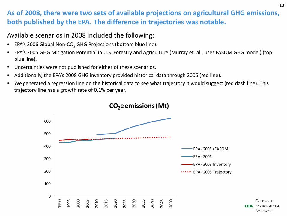
As of 2008, there were two sets of available projections on agricultural GHG emissions, both published by the EPA. The difference in trajectories was notable.
Available scenarios in 2008 included the following: • EPA’s 2006 Global Non-CO2 GHG Projections (bottom blue line).
• EPA’s 2005 GHG Mitigation Potential in U.S. Forestry and Agriculture (Murray et. al., uses FASOM GHG model) (top blue line).
• Uncertainties were not published for either of these scenarios.
• Additionally, the EPA’s 2008 GHG inventory provided historical data through 2006 (red line).
• We generated a regression line on the historical data to see what trajectory it would suggest (red dash line). This trajectory line has a growth rate of 0.1% per year.
13
0
100
200
300
400
500
600
1990
1995
2000
2005
2010
2015
2020
2025
2030
2035
2040
2045
2050
CO2e emissions (Mt)
EPA - 2005 (FASOM)
EPA - 2006
EPA - 2008 Inventory
EPA - 2008 Trajectory
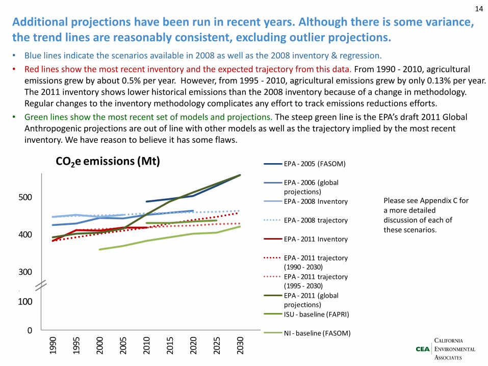
Additional projections have been run in recent years. Although there is some variance, the trend lines are reasonably consistent, excluding outlier projections.
• Blue lines indicate the scenarios available in 2008 as well as the 2008 inventory & regression.
• Red lines show the most recent inventory and the expected trajectory from this data. From 1990 - 2010, agricultural emissions grew by about 0.5% per year. However, from 1995 - 2010, agricultural emissions grew by only 0.13% per year. The 2011 inventory shows lower historical emissions than the 2008 inventory because of a change in methodology. Regular changes to the inventory methodology complicates any effort to track emissions reductions efforts.
• Green lines show the most recent set of models and projections. The steep green line is the EPA’s draft 2011 Global Anthropogenic projections are out of line with other models as well as the trajectory implied by the most recent inventory. We have reason to believe it has some flaws.
14
0
100
200
300
400
500
1990
1995
2000
2005
2010
2015
2020
2025
2030
CO2e emissions (Mt)EPA - 2005 (FASOM)
EPA - 2006 (global projections)
EPA - 2008 Inventory
EPA - 2008 trajectory
EPA - 2011 Inventory
EPA - 2011 trajectory (1990 - 2030)
EPA - 2011 trajectory (1995 - 2030)
EPA - 2011 (global projections)
ISU - baseline (FAPRI)
NI - baseline (FASOM) 0
100
200
300
400
500
1990
1995
2000
2005
2010
2015
2020
2025
2030
CO2e emissions (Mt)EPA - 2005 (FASOM)
EPA - 2006 (global projections)
EPA - 2008 Inventory
EPA - 2008 trajectory
EPA - 2011 Inventory
EPA - 2011 trajectory (1990 - 2030)
EPA - 2011 trajectory (1995 - 2030)
EPA - 2011 (global projections)
ISU - baseline (FAPRI)
NI - baseline (FASOM)
0
100
200
300
400
500
1990
1995
2000
2005
2010
2015
2020
2025
2030
CO2e emissions (Mt)EPA - 2005 (FASOM)
EPA - 2006 (global projections)
EPA - 2008 Inventory
EPA - 2008 trajectory
EPA - 2011 Inventory
EPA - 2011 trajectory (1990 - 2030)
EPA - 2011 trajectory (1995 - 2030)
EPA - 2011 (global projections)
ISU - baseline (FAPRI)
NI - baseline (FASOM)
Please see Appendix C for a more detailed discussion of each of these scenarios.
489
453 455431
384
419
-75
25
125
225
325
425
525
625
EPA - 2005 (FASOM) EPA - 2006 (global projections)
EPA - 2011 (global projections)
ISU - baseline (FAPRI) NI - baseline (FASOM) EPA Inventory (2009)
2010 emissions (Mt CO2e)
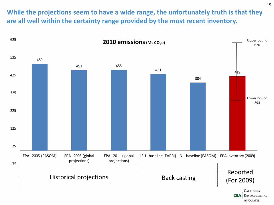
While the projections seem to have a wide range, the unfortunately truth is that they are all well within the certainty range provided by the most recent inventory.
Historical projections Back casting Reported (For 2009)
15
Upper bound 620
Lower bound 293
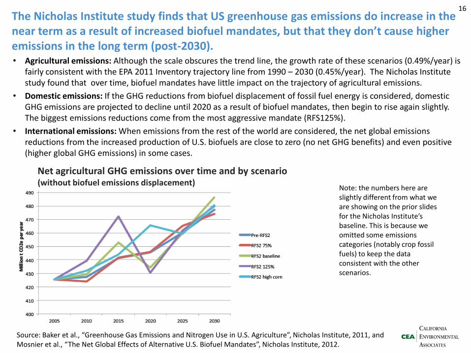
The Nicholas Institute study finds that US greenhouse gas emissions do increase in the near term as a result of increased biofuel mandates, but that they don’t cause higher emissions in the long term (post-2030).
16
Source: Baker et al., “Greenhouse Gas Emissions and Nitrogen Use in U.S. Agriculture”, Nicholas Institute, 2011, and Mosnier et al., “The Net Global Effects of Alternative U.S. Biofuel Mandates”, Nicholas Institute, 2012.
Net agricultural GHG emissions over time and by scenario (without biofuel emissions displacement)
• Agricultural emissions: Although the scale obscures the trend line, the growth rate of these scenarios (0.49%/year) is fairly consistent with the EPA 2011 Inventory trajectory line from 1990 – 2030 (0.45%/year). The Nicholas Institute study found that over time, biofuel mandates have little impact on the trajectory of agricultural emissions.
• Domestic emissions: If the GHG reductions from biofuel displacement of fossil fuel energy is considered, domestic GHG emissions are projected to decline until 2020 as a result of biofuel mandates, then begin to rise again slightly. The biggest emissions reductions come from the most aggressive mandate (RFS125%).
• International emissions: When emissions from the rest of the world are considered, the net global emissions reductions from the increased production of U.S. biofuels are close to zero (no net GHG benefits) and even positive (higher global GHG emissions) in some cases.
Note: the numbers here are slightly different from what we are showing on the prior slides for the Nicholas Institute’s baseline. This is because we omitted some emissions categories (notably crop fossil fuels) to keep the data consistent with the other scenarios.
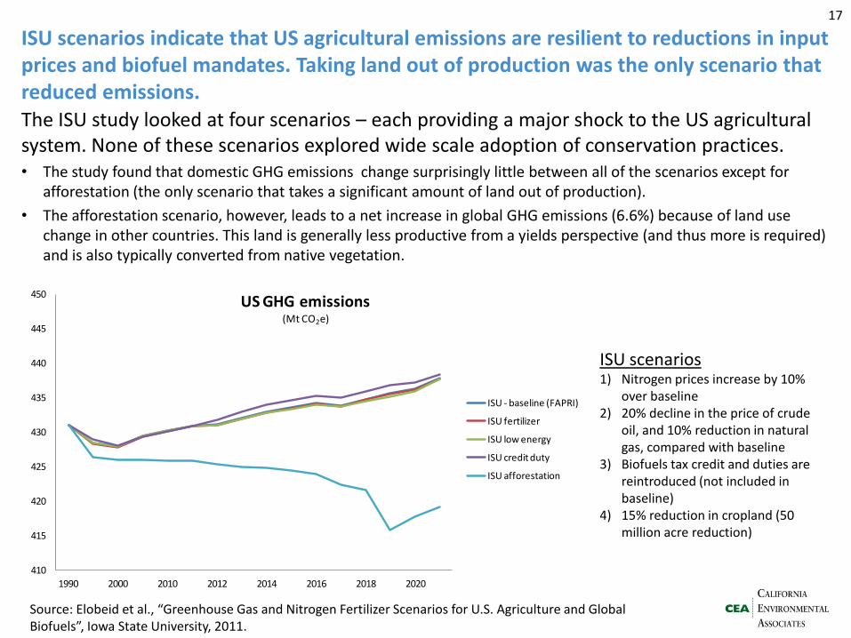
ISU scenarios indicate that US agricultural emissions are resilient to reductions in input prices and biofuel mandates. Taking land out of production was the only scenario that reduced emissions. The ISU study looked at four scenarios – each providing a major shock to the US agricultural system. None of these scenarios explored wide scale adoption of conservation practices. • The study found that domestic GHG emissions change surprisingly little between all of the scenarios except for
afforestation (the only scenario that takes a significant amount of land out of production).
• The afforestation scenario, however, leads to a net increase in global GHG emissions (6.6%) because of land use change in other countries. This land is generally less productive from a yields perspective (and thus more is required) and is also typically converted from native vegetation.
ISU scenarios 1) Nitrogen prices increase by 10%
over baseline 2) 20% decline in the price of crude
oil, and 10% reduction in natural gas, compared with baseline
3) Biofuels tax credit and duties are reintroduced (not included in baseline)
4) 15% reduction in cropland (50 million acre reduction)
17
Source: Elobeid et al., “Greenhouse Gas and Nitrogen Fertilizer Scenarios for U.S. Agriculture and Global Biofuels”, Iowa State University, 2011.
410
415
420
425
430
435
440
445
450
1990 2000 2010 2012 2014 2016 2018 2020
US GHG emissions (Mt CO2e)
ISU - baseline (FAPRI)
ISU fertilizer
ISU low energy
ISU credit duty
ISU afforestation
0
50
100
150
200
250
300
350
400
450
500
1990 1995 2000 2005 2008
CO2e emissions (Mt)
EPA 2011 - no carbon
USDA 2011 - no carbon
USDA 2011 - with carbon (gross)
USDA 2011 - with carbon (net)
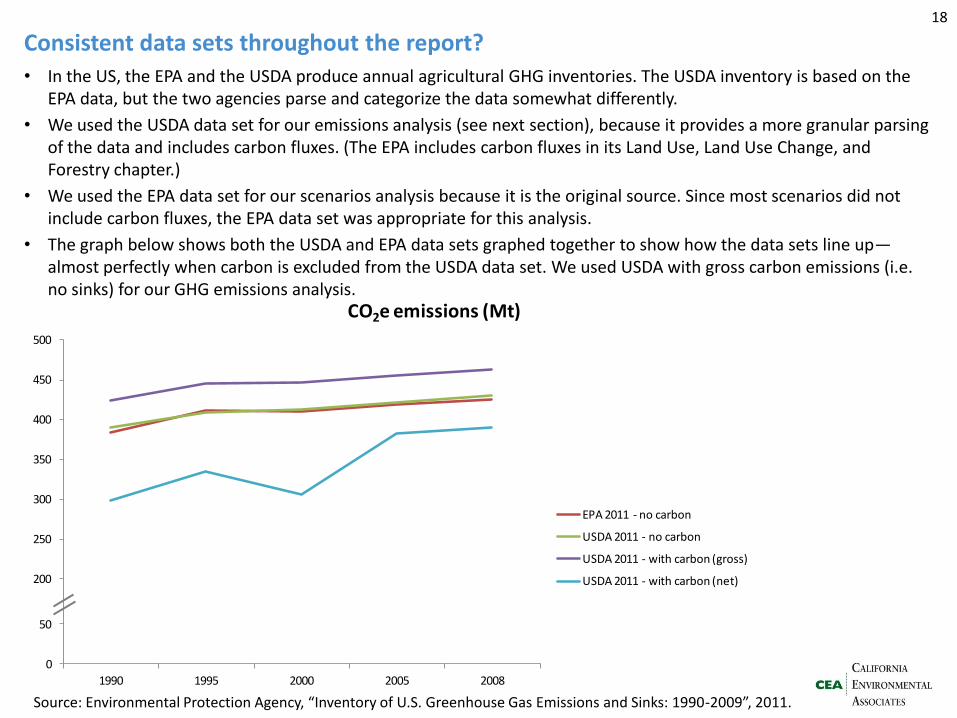
Consistent data sets throughout the report? 18
Source: Environmental Protection Agency, “Inventory of U.S. Greenhouse Gas Emissions and Sinks: 1990-2009”, 2011.
0
50
100
150
200
250
300
350
400
450
500
1990 1995 2000 2005 2008
CO2e emissions (Mt)
EPA 2011 - no carbon
USDA 2011 - no carbon
USDA 2011 - with carbon (gross)
USDA 2011 - with carbon (net)
• In the US, the EPA and the USDA produce annual agricultural GHG inventories. The USDA inventory is based on the EPA data, but the two agencies parse and categorize the data somewhat differently.
• We used the USDA data set for our emissions analysis (see next section), because it provides a more granular parsing of the data and includes carbon fluxes. (The EPA includes carbon fluxes in its Land Use, Land Use Change, and Forestry chapter.)
• We used the EPA data set for our scenarios analysis because it is the original source. Since most scenarios did not include carbon fluxes, the EPA data set was appropriate for this analysis.
• The graph below shows both the USDA and EPA data sets graphed together to show how the data sets line up—almost perfectly when carbon is excluded from the USDA data set. We used USDA with gross carbon emissions (i.e. no sinks) for our GHG emissions analysis.
GHG Emissions Executive summary > GHG emissions > GHG mitigation > Nitrogen pollution > Nitrogen mitigation
- Scenarios - Global and national context - US agricultural emissions
overview - Livestock - Croplands
19
Section summary: The sources of agricultural emissions—both by commodity and geography—are fairly stable. The leading commodities are corn and cattle (both beef and dairy), and the leading regions are the Midwest, Texas, and California.
• Emissions are roughly split 60/40 between livestock and crops . N2O emissions from agricultural soils (~33%) and enteric fermentation from livestock (~30%) are the two biggest overall contributors.
• Corn is the leading commodity crop contributor because it has the largest acreage and the greatest emissions on a per acre basis due to its intensive use of nitrogen fertilizer.
• Soil carbon in cropped and grazed lands can function as either a source or a sink, depending on weather, usage patterns, and management of the land. Soil carbon from croplands has served as a small net sink in recent years, reducing overall agricultural emissions by approximately 10% per year since 2003.
• Emissions from the manure of dairy cattle and swine have grown notably. Between 1990 and 2008, emissions from dairy cattle grew 26% and emissions from swine grew 46%.
• Dairy cattle have the highest emissions per head and are the only animal whose emissions per head has increased significantly in the last 20 years.
• The states with the highest agricultural GHG emissions are Texas (40 Mt CO2e/yr), Iowa (30 Mt CO2e/yr), and California (27 Mt CO2e/yr).
20
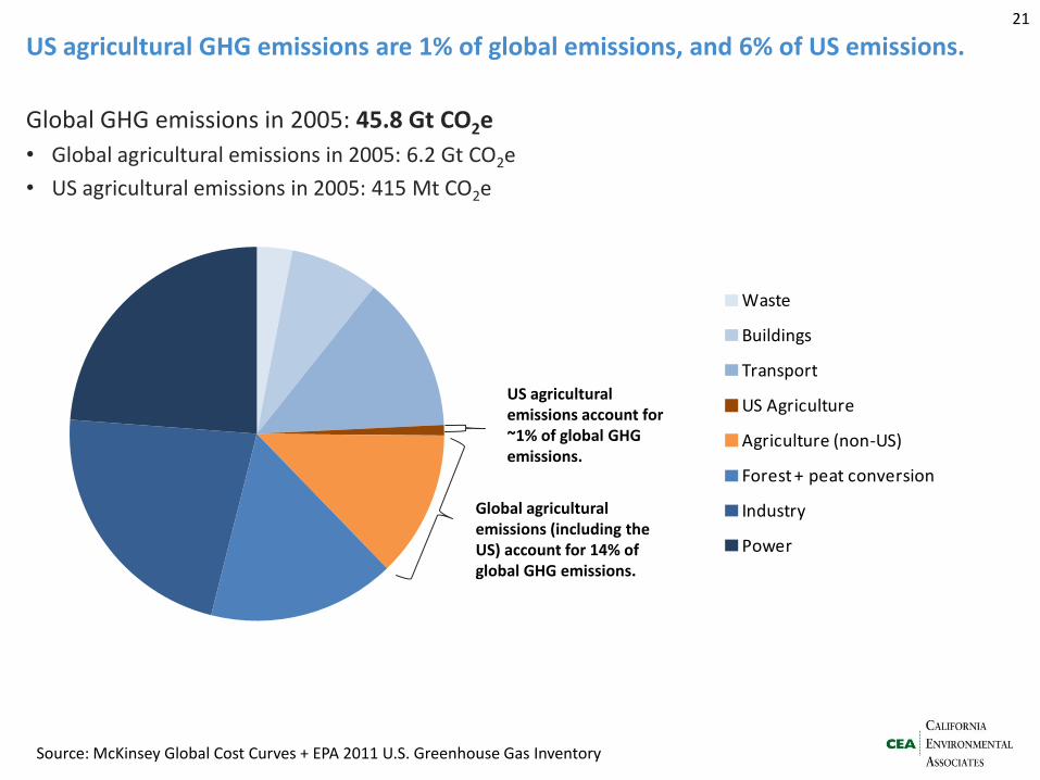
US agricultural GHG emissions are 1% of global emissions, and 6% of US emissions.
Global GHG emissions in 2005: 45.8 Gt CO2e
• Global agricultural emissions in 2005: 6.2 Gt CO2e
• US agricultural emissions in 2005: 415 Mt CO2e
Source: McKinsey Global Cost Curves + EPA 2011 U.S. Greenhouse Gas Inventory
Waste
Buildings
Transport
US Agriculture
Agriculture (non-US)
Forest + peat conversion
Industry
Power
Waste
Buildings
Transport
US Agriculture
Agriculture (non-US)
Forest + peat conversion
Industry
Power
US agricultural emissions account for ~1% of global GHG emissions.
21
Global agricultural emissions (including the US) account for 14% of global GHG emissions.
-2,000
-1,000
0
1,000
2,000
3,000
4,000
5,000
6,000
7,000
8,000
1990 1995 2000 2005 2008
Land Use, Land-Use Change, and Forestry (Sinks)
U.S. Territories
Residential
Commercial
Agriculture
Industry
Transportation
Electric Power Industry
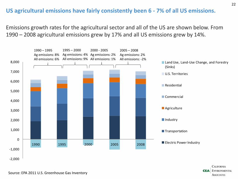
US agricultural emissions have fairly consistently been 6 - 7% of all US emissions.
Emissions growth rates for the agricultural sector and all of the US are shown below. From 1990 – 2008 agricultural emissions grew by 17% and all US emissions grew by 14%.
Source: EPA 2011 U.S. Greenhouse Gas Inventory
1990 – 1995 Ag emissions: 8% All emissions: 6%
1995 – 2000 Ag emissions: 4% All emissions: 9%
2000 - 2005 Ag emissions: 2% All emissions: 1%
2005 – 2008 Ag emissions: 2% All emissions: -2%
22
GHG Emissions Executive summary > GHG emissions > GHG mitigation > Nitrogen pollution > Nitrogen mitigation
- Scenarios - Global and national context - US agricultural emissions overview - Livestock - Croplands
23
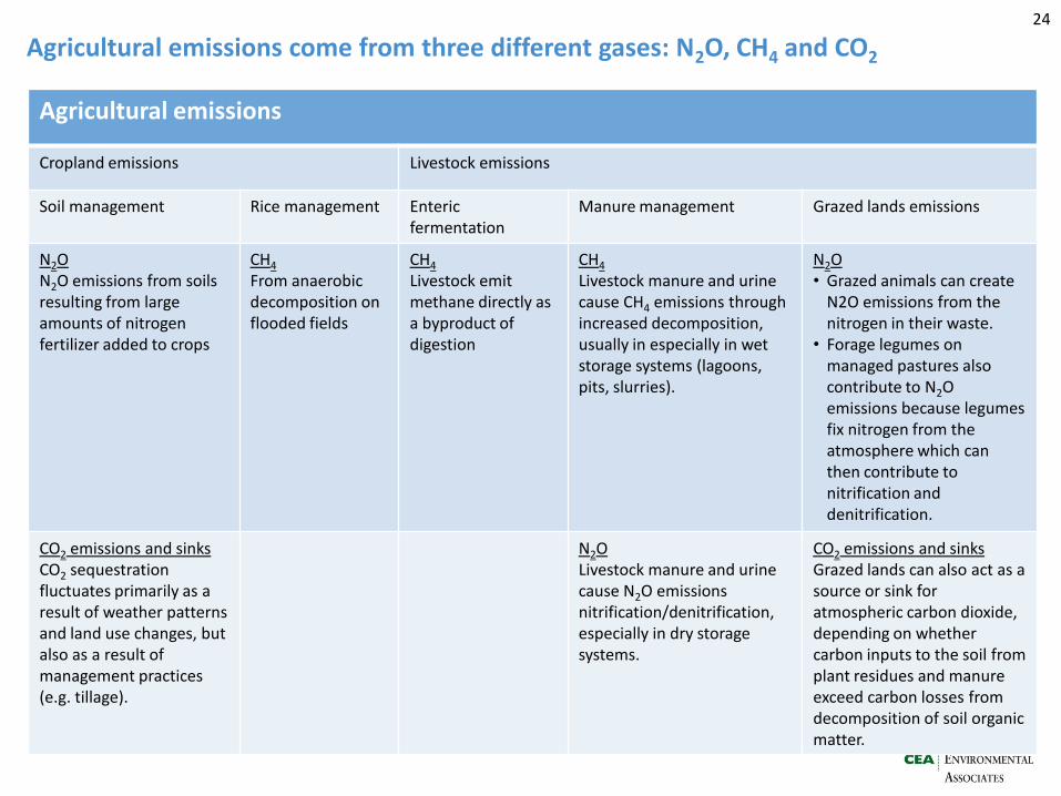
Agricultural emissions come from three different gases: N2O, CH4 and CO2 24
Agricultural emissions
Cropland emissions Livestock emissions
Soil management Rice management Enteric fermentation
Manure management Grazed lands emissions
N2O N2O emissions from soils resulting from large amounts of nitrogen fertilizer added to crops
CH4 From anaerobic decomposition on flooded fields
CH4 Livestock emit methane directly as a byproduct of digestion
CH4 Livestock manure and urine cause CH4 emissions through increased decomposition, usually in especially in wet storage systems (lagoons, pits, slurries).
N2O • Grazed animals can create
N2O emissions from the nitrogen in their waste.
• Forage legumes on managed pastures also contribute to N2O emissions because legumes fix nitrogen from the atmosphere which can then contribute to nitrification and denitrification.
CO2 emissions and sinks CO2 sequestration fluctuates primarily as a result of weather patterns and land use changes, but also as a result of management practices (e.g. tillage).
N2O Livestock manure and urine cause N2O emissions nitrification/denitrification, especially in dry storage systems.
CO2 emissions and sinks Grazed lands can also act as a source or sink for atmospheric carbon dioxide, depending on whether carbon inputs to the soil from plant residues and manure exceed carbon losses from decomposition of soil organic matter.
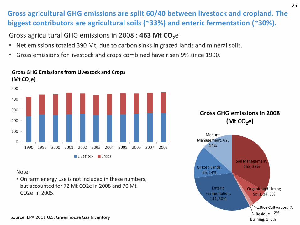
Gross agricultural GHG emissions are split 60/40 between livestock and cropland. The biggest contributors are agricultural soils (~33%) and enteric fermentation (~30%).
Gross agricultural GHG emissions in 2008 : 463 Mt CO2e
• Net emissions totaled 390 Mt, due to carbon sinks in grazed lands and mineral soils.
• Gross emissions for livestock and crops combined have risen 9% since 1990.
Source: EPA 2011 U.S. Greenhouse Gas Inventory
25
Gross GHG emissions in 2008 (Mt CO2e)
Soil Management, 153, 33%
Organic and Liming Soils, 34, 7%
Rice Cultivation, 7, 2%Residue
Burning, 1, 0%
Enteric Fermentation,
141, 30%
Grazed Lands, 65, 14%
Manure Management, 62,
14%
Gross GHG Emissions from Crops and Livestock in 2008(Mt CO2e)
Note: • On farm energy use is not included in these numbers,
but accounted for 72 Mt CO2e in 2008 and 70 Mt CO2e in 2005.
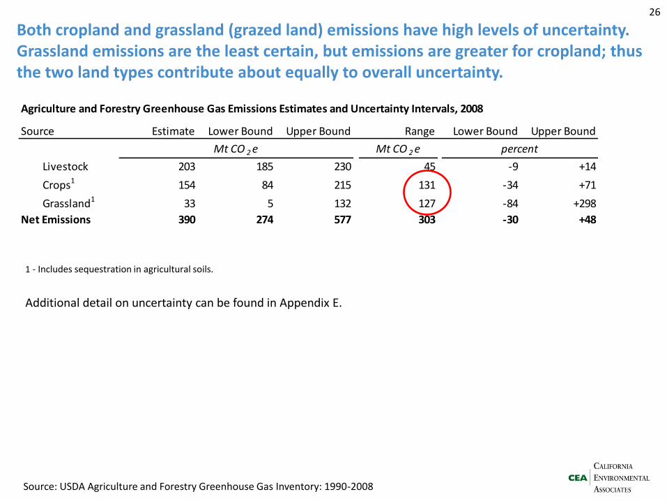
Agriculture and Forestry Greenhouse Gas Emissions Estimates and Uncertainty Intervals, 2008
Source Estimate Lower Bound Upper Bound Range Lower Bound Upper Bound
Mt CO 2 e
Livestock 203 185 230 45 -9 +14
Crops1 154 84 215 131 -34 +71
Grassland1 33 5 132 127 -84 +298
Net Emissions 390 274 577 303 -30 +48
Mt CO 2 e percent
Both cropland and grassland (grazed land) emissions have high levels of uncertainty. Grassland emissions are the least certain, but emissions are greater for cropland; thus the two land types contribute about equally to overall uncertainty.
1 - Includes sequestration in agricultural soils.
Source: USDA Agriculture and Forestry Greenhouse Gas Inventory: 1990-2008
26
Additional detail on uncertainty can be found in Appendix E.
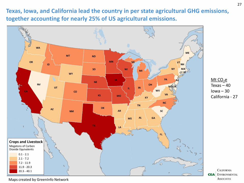
Texas, Iowa, and California lead the country in per state agricultural GHG emissions, together accounting for nearly 25% of US agricultural emissions.
27
Mt CO2e Texas – 40 Iowa – 30 California - 27
Maps created by GreenInfo Network

GHG Emissions Executive summary > GHG emissions > GHG mitigation > Nitrogen pollution > Nitrogen mitigation
- Scenarios - Global and national context - US agricultural emissions overview - Livestock - Croplands
28
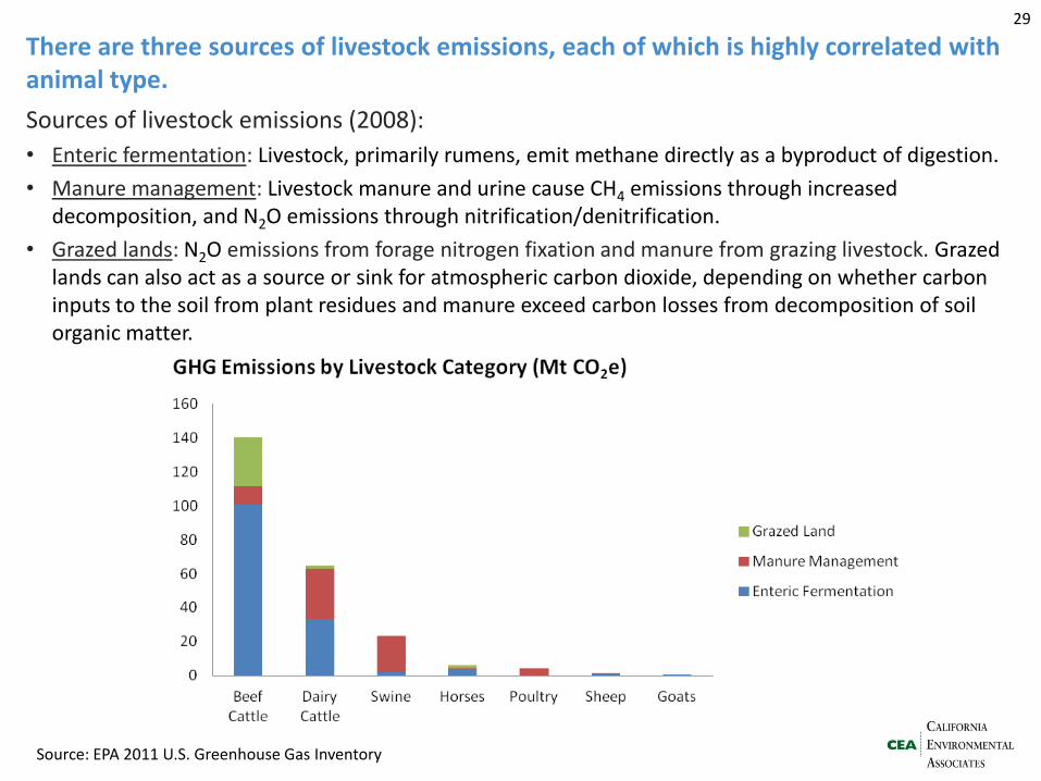
There are three sources of livestock emissions, each of which is highly correlated with animal type.
Sources of livestock emissions (2008):
• Enteric fermentation: Livestock, primarily rumens, emit methane directly as a byproduct of digestion.
• Manure management: Livestock manure and urine cause CH4 emissions through increased decomposition, and N2O emissions through nitrification/denitrification.
• Grazed lands: N2O emissions from forage nitrogen fixation and manure from grazing livestock. Grazed lands can also act as a source or sink for atmospheric carbon dioxide, depending on whether carbon inputs to the soil from plant residues and manure exceed carbon losses from decomposition of soil organic matter.
Source: EPA 2011 U.S. Greenhouse Gas Inventory
29
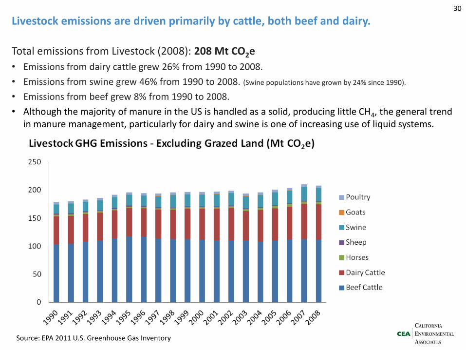
Livestock emissions are driven primarily by cattle, both beef and dairy.
Total emissions from Livestock (2008): 208 Mt CO2e
• Emissions from dairy cattle grew 26% from 1990 to 2008.
• Emissions from swine grew 46% from 1990 to 2008. (Swine populations have grown by 24% since 1990).
• Emissions from beef grew 8% from 1990 to 2008.
• Although the majority of manure in the US is handled as a solid, producing little CH4, the general trend in manure management, particularly for dairy and swine is one of increasing use of liquid systems.
Source: EPA 2011 U.S. Greenhouse Gas Inventory
30
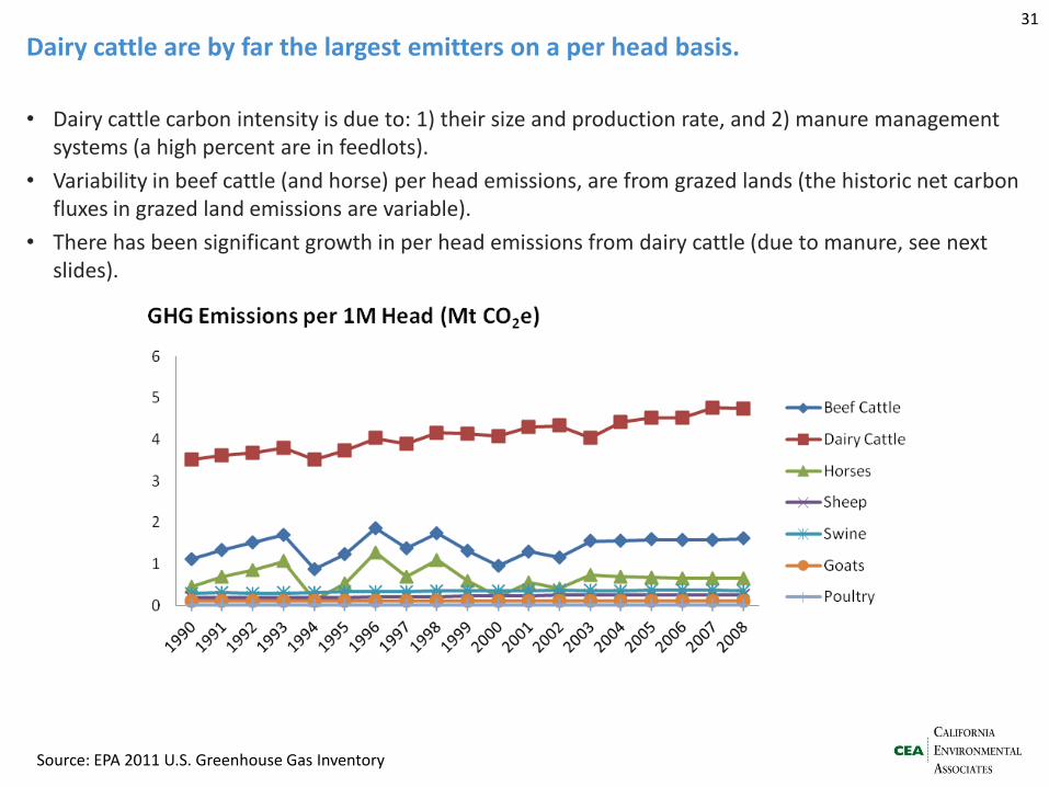
Dairy cattle are by far the largest emitters on a per head basis.
• Dairy cattle carbon intensity is due to: 1) their size and production rate, and 2) manure management systems (a high percent are in feedlots).
• Variability in beef cattle (and horse) per head emissions, are from grazed lands (the historic net carbon fluxes in grazed land emissions are variable).
• There has been significant growth in per head emissions from dairy cattle (due to manure, see next slides).
Source: EPA 2011 U.S. Greenhouse Gas Inventory
31
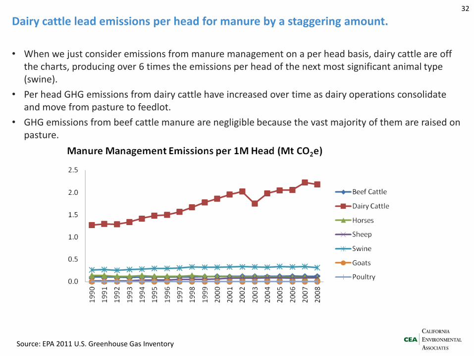
Dairy cattle lead emissions per head for manure by a staggering amount.
• When we just consider emissions from manure management on a per head basis, dairy cattle are off the charts, producing over 6 times the emissions per head of the next most significant animal type (swine).
• Per head GHG emissions from dairy cattle have increased over time as dairy operations consolidate and move from pasture to feedlot.
• GHG emissions from beef cattle manure are negligible because the vast majority of them are raised on pasture.
Source: EPA 2011 U.S. Greenhouse Gas Inventory
32
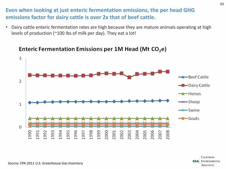
Even when looking at just enteric fermentation emissions, the per head GHG emissions factor for dairy cattle is over 2x that of beef cattle.
• Dairy cattle enteric fermentation rates are high because they are mature animals operating at high levels of production (~100 lbs of milk per day). They eat a lot!
Source: EPA 2011 U.S. Greenhouse Gas Inventory
33
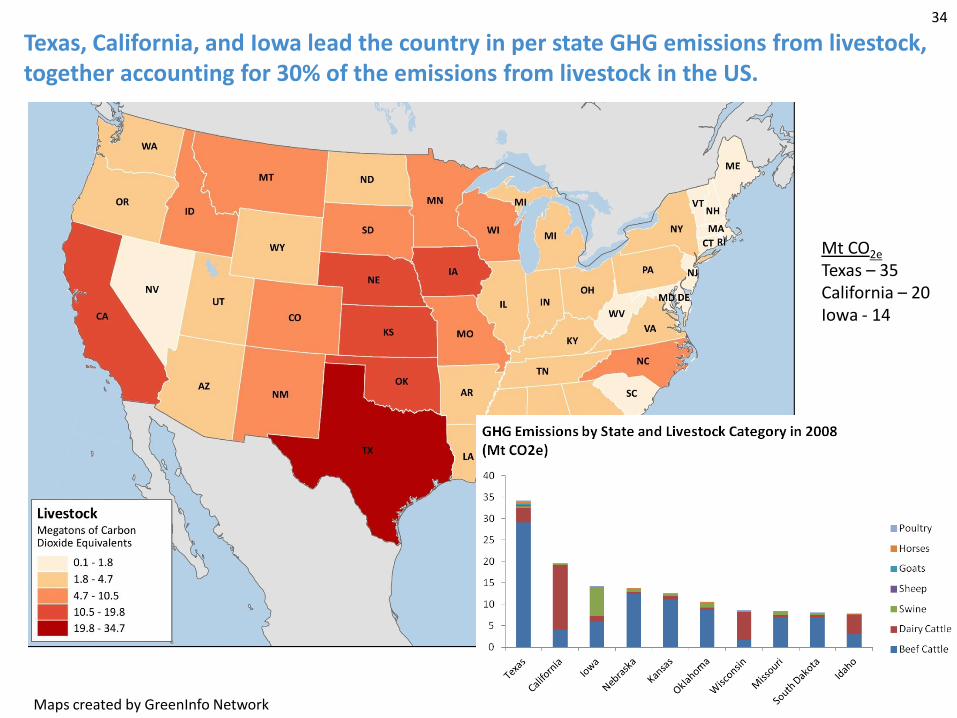
Texas, California, and Iowa lead the country in per state GHG emissions from livestock, together accounting for 30% of the emissions from livestock in the US.
34
Mt CO2e
Texas – 35 California – 20 Iowa - 14
Maps created by GreenInfo Network
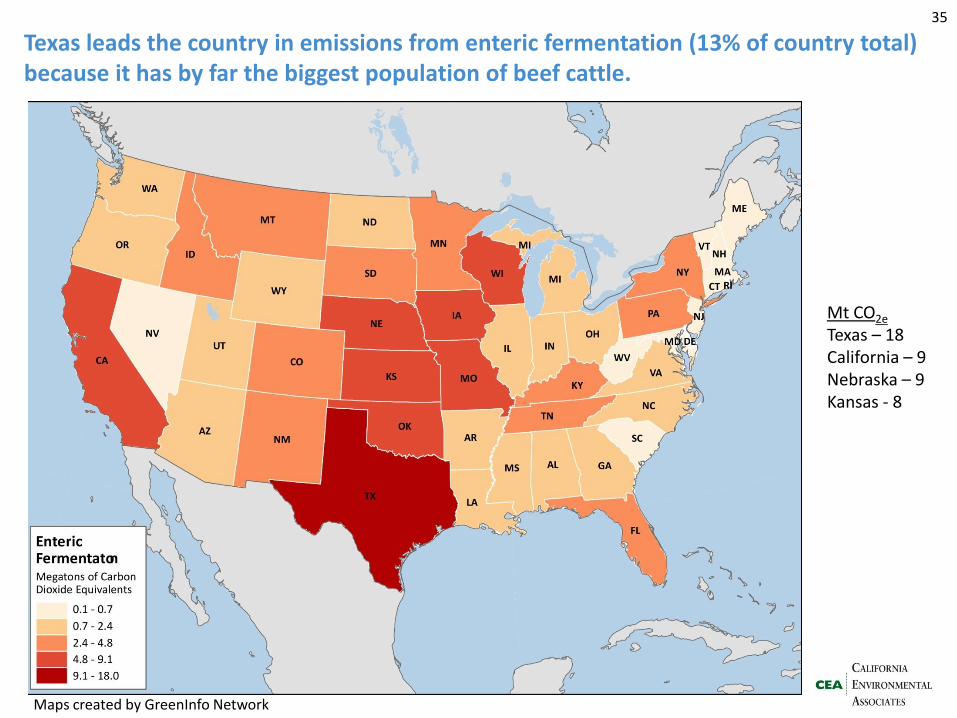
Texas leads the country in emissions from enteric fermentation (13% of country total) because it has by far the biggest population of beef cattle.
35
Mt CO2e
Texas – 18 California – 9 Nebraska – 9 Kansas - 8
Maps created by GreenInfo Network
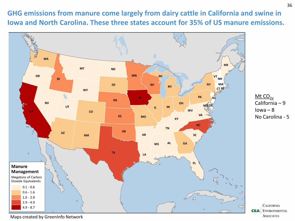
GHG emissions from manure come largely from dairy cattle in California and swine in Iowa and North Carolina. These three states account for 35% of US manure emissions.
36
Mt CO2e
California – 9 Iowa – 8 No Carolina - 5
Maps created by GreenInfo Network
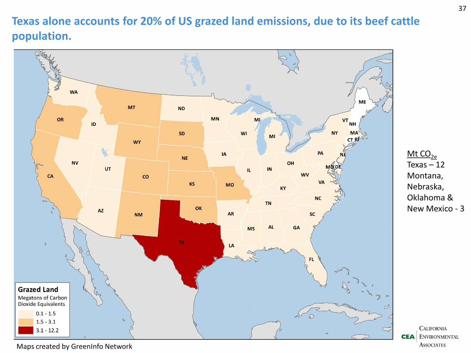
Texas alone accounts for 20% of US grazed land emissions, due to its beef cattle population.
37
Mt CO2e
Texas – 12 Montana, Nebraska, Oklahoma & New Mexico - 3
Maps created by GreenInfo Network
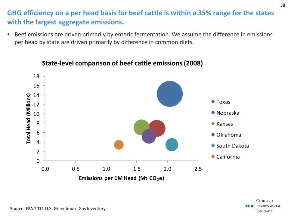
GHG efficiency on a per head basis for beef cattle is within a 35% range for the states with the largest aggregate emissions.
Source: EPA 2011 U.S. Greenhouse Gas Inventory
38
State-level comparison of beef cattle emissions (2008)
• Beef emissions are driven primarily by enteric fermentation. We assume the difference in emissions per head by state are driven primarily by difference in common diets.
0
2
4
6
8
10
12
14
16
18
0.0 0.5 1.0 1.5 2.0 2.5
Tota
l He
ad (
Mill
ion
s)
Emissions per 1M Head (Mt CO2e)
Emissions per Head, Total Head, and Total Emissions for Beef Cattle
Texas
Nebraska
Kansas
Oklahoma
South Dakota
California
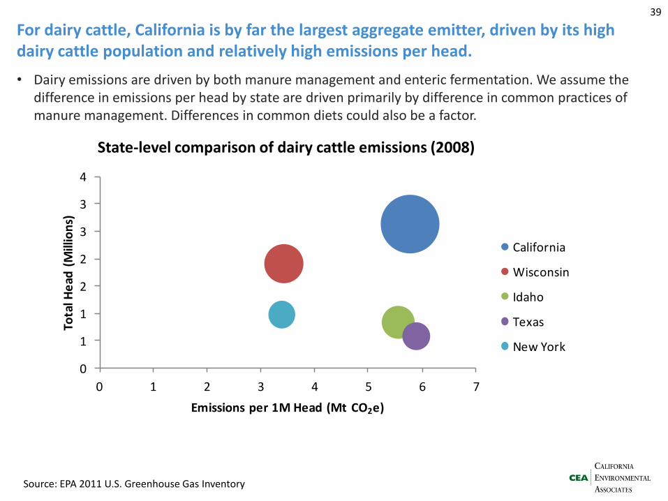
• Dairy emissions are driven by both manure management and enteric fermentation. We assume the difference in emissions per head by state are driven primarily by difference in common practices of manure management. Differences in common diets could also be a factor.
For dairy cattle, California is by far the largest aggregate emitter, driven by its high dairy cattle population and relatively high emissions per head.
Source: EPA 2011 U.S. Greenhouse Gas Inventory
39
State-level comparison of dairy cattle emissions (2008)
0
1
1
2
2
3
3
4
0 1 2 3 4 5 6 7
Tota
l He
ad (
Mill
ion
s)
Emissions per 1M Head (Mt CO2e)
Emissions per Head, Total Head, and Total Emissions for Dairy Cattle
California
Wisconsin
Idaho
Texas
New York
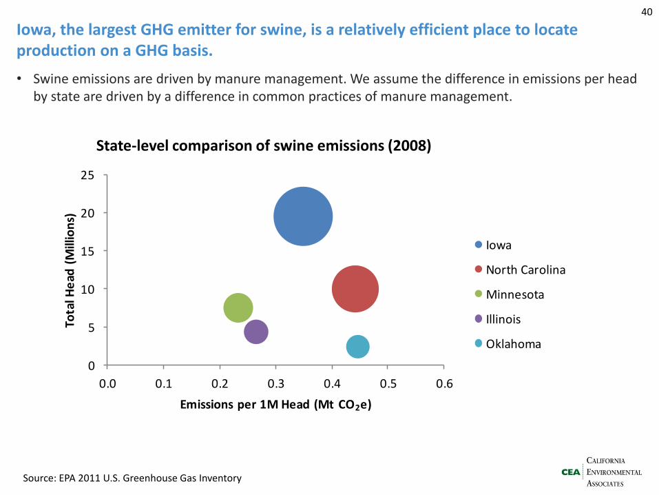
• Swine emissions are driven by manure management. We assume the difference in emissions per head by state are driven by a difference in common practices of manure management.
Iowa, the largest GHG emitter for swine, is a relatively efficient place to locate production on a GHG basis.
Source: EPA 2011 U.S. Greenhouse Gas Inventory
40
State-level comparison of swine emissions (2008)
0
5
10
15
20
25
0.0 0.1 0.2 0.3 0.4 0.5 0.6
Tota
l He
ad (
Mill
ion
s)
Emissions per 1M Head (Mt CO2e)
Emissions per Head, Total Head, and Total Emissions for Swine
Iowa
North Carolina
Minnesota
Illinois
Oklahoma
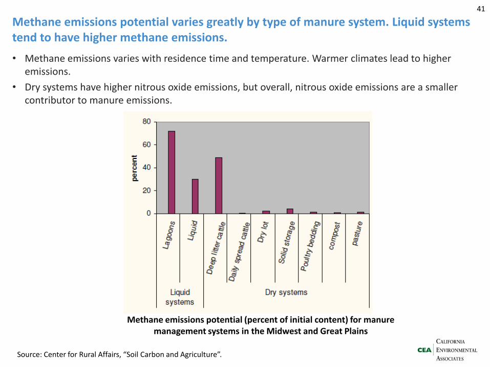
Methane emissions potential varies greatly by type of manure system. Liquid systems tend to have higher methane emissions.
41
Source: Center for Rural Affairs, “Soil Carbon and Agriculture”.
• Methane emissions varies with residence time and temperature. Warmer climates lead to higher emissions.
• Dry systems have higher nitrous oxide emissions, but overall, nitrous oxide emissions are a smaller contributor to manure emissions.
Methane emissions potential (percent of initial content) for manure management systems in the Midwest and Great Plains
GHG Emissions Executive summary > GHG emissions > GHG mitigation > Nitrogen pollution > Nitrogen mitigation
- Scenarios - Global and national context - US agricultural emissions overview - Livestock - Croplands
42
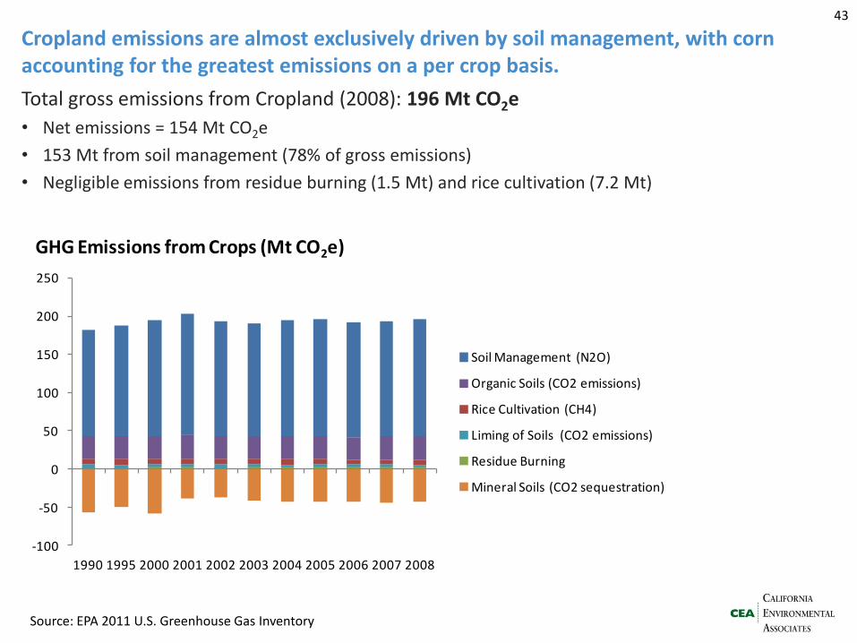
Cropland emissions are almost exclusively driven by soil management, with corn accounting for the greatest emissions on a per crop basis.
Source: EPA 2011 U.S. Greenhouse Gas Inventory
Total gross emissions from Cropland (2008): 196 Mt CO2e
• Net emissions = 154 Mt CO2e
• 153 Mt from soil management (78% of gross emissions)
• Negligible emissions from residue burning (1.5 Mt) and rice cultivation (7.2 Mt)
43
-100
-50
0
50
100
150
200
250
1990 1995 2000 2001 2002 2003 2004 2005 2006 2007 2008
GHG Emissions from Crops (Mt CO2e)
Soil Management (N2O)
Organic Soils (CO2 emissions)
Rice Cultivation (CH4)
Liming of Soils (CO2 emissions)
Residue Burning
Mineral Soils (CO2 sequestration)
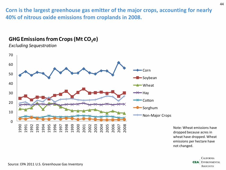
Corn is the largest greenhouse gas emitter of the major crops, accounting for nearly 40% of nitrous oxide emissions from croplands in 2008.
44
0
10
20
30
40
50
60
70
19
90
19
91
19
92
19
93
19
94
19
95
19
96
19
97
19
98
19
99
20
00
20
01
20
02
20
03
20
04
20
05
20
06
20
07
20
08
GHG Emissions from Crops (Mt CO2e)Excluding Sequestration
Corn
Soybean
Wheat
Hay
Cotton
Sorghum
Non-Major Crops
Source: EPA 2011 U.S. Greenhouse Gas Inventory
Note: Wheat emissions have dropped because acres in wheat have dropped. Wheat emissions per hectare have not changed.
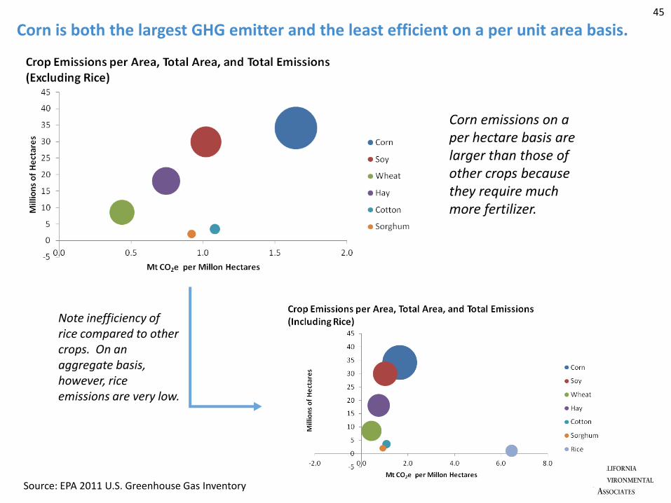
Corn is both the largest GHG emitter and the least efficient on a per unit area basis.
Source: EPA 2011 U.S. Greenhouse Gas Inventory
45
Note inefficiency of rice compared to other crops. On an aggregate basis, however, rice emissions are very low.
Corn emissions on a per hectare basis are larger than those of other crops because they require much more fertilizer.
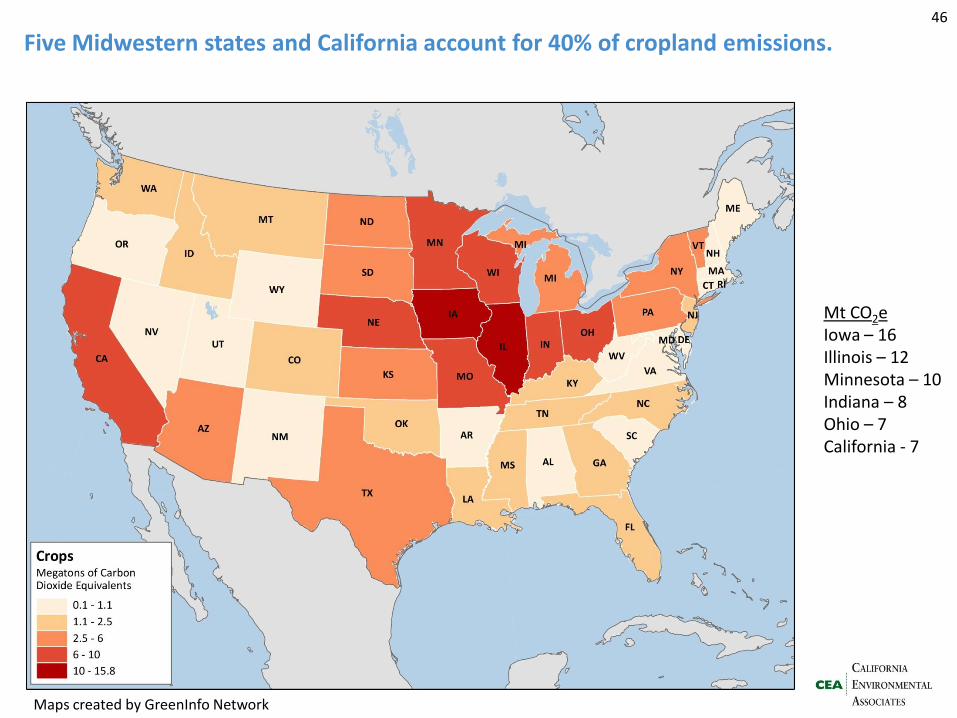
Five Midwestern states and California account for 40% of cropland emissions. 46
Mt CO2e
Iowa – 16 Illinois – 12 Minnesota – 10 Indiana – 8 Ohio – 7 California - 7
Maps created by GreenInfo Network
GHG Mitigation Executive summary > GHG emissions > GHG mitigation > Nitrogen pollution > Nitrogen mitigation
- Logic model - Literature review - Deep dive on croplands & grasslands - Livestock - Regional distribution - Economics
47
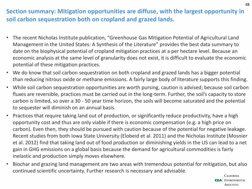
Section summary: Mitigation opportunities are diffuse, with the largest opportunity in soil carbon sequestration both on cropland and grazed lands.
• The recent Nicholas Institute publication, “Greenhouse Gas Mitigation Potential of Agricultural Land Management in the United States: A Synthesis of the Literature” provides the best data summary to date on the biophysical potential of cropland mitigation practices at a per hectare level. Because an economic analysis at the same level of granularity does not exist, it is difficult to evaluate the economic potential of these mitigation practices.
• We do know that soil carbon sequestration on both cropland and grazed lands has a bigger potential than reducing nitrous oxide or methane emissions. A fairly large body of literature supports this finding.
• While soil carbon sequestration opportunities are worth pursing, caution is advised; because soil carbon fluxes are reversible, practices must be carried out in the long-term. Further, the soil’s capacity to store carbon is limited, so over a 30 - 50 year time horizon, the soils will become saturated and the potential to sequester will diminish on an annual basis.
• Practices that require taking land out of production, or significantly reduce productivity, have a high opportunity cost and thus are only viable if there is economic compensation (e.g. a high price on carbon). Even then, they should be pursued with caution because of the potential for negative leakage. Recent studies from both Iowa State University (Elobeid et al. 2011) and the Nicholas Institute (Mosnier et al. 2012) find that taking land out of food production or diminishing yields in the US can lead to a net gain in GHG emissions on a global basis because the demand for agricultural commodities is fairly inelastic and production simply moves elsewhere.
• Biochar and grazing land management are two areas with tremendous potential for mitigation, but also continued scientific uncertainty. Further research is necessary and advisable.
48
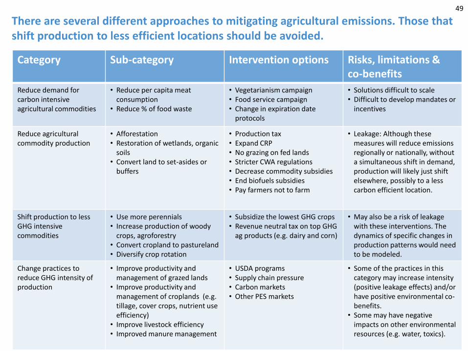
There are several different approaches to mitigating agricultural emissions. Those that shift production to less efficient locations should be avoided.
Category Sub-category Intervention options Risks, limitations & co-benefits
Reduce demand for carbon intensive agricultural commodities
• Reduce per capita meat consumption
• Reduce % of food waste
• Vegetarianism campaign • Food service campaign • Change in expiration date
protocols
• Solutions difficult to scale • Difficult to develop mandates or
incentives
Reduce agricultural commodity production
• Afforestation • Restoration of wetlands, organic
soils • Convert land to set-asides or
buffers
• Production tax • Expand CRP • No grazing on fed lands • Stricter CWA regulations • Decrease commodity subsidies • End biofuels subsidies • Pay farmers not to farm
• Leakage: Although these measures will reduce emissions regionally or nationally, without a simultaneous shift in demand, production will likely just shift elsewhere, possibly to a less carbon efficient location.
Shift production to less GHG intensive commodities
• Use more perennials • Increase production of woody
crops, agroforestry • Convert cropland to pastureland • Diversify crop rotation
• Subsidize the lowest GHG crops • Revenue neutral tax on top GHG
ag products (e.g. dairy and corn)
• May also be a risk of leakage with these interventions. The dynamics of specific changes in production patterns would need to be modeled.
Change practices to reduce GHG intensity of production
• Improve productivity and management of grazed lands
• Improve productivity and management of croplands (e.g. tillage, cover crops, nutrient use efficiency)
• Improve livestock efficiency • Improved manure management
• USDA programs • Supply chain pressure • Carbon markets • Other PES markets
• Some of the practices in this category may increase intensity (positive leakage effects) and/or have positive environmental co-benefits.
• Some may have negative impacts on other environmental resources (e.g. water, toxics).
49
GHG Mitigation Executive summary > GHG emissions > GHG mitigation > Nitrogen pollution > Nitrogen mitigation
- Logic model - Literature review - Deep dive on croplands & grasslands - Livestock - Regional distribution - Economics
50
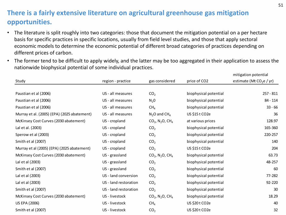
There is a fairly extensive literature on agricultural greenhouse gas mitigation opportunities.
51
Study region - practice gas considered price of CO2
mitigation potential
estimate (Mt CO2e / yr)
Paustian et al (2006) US - all measures CO2 biophysical potential 257 - 811
Paustian et al (2006) US - all measures N20 biophysical potential 84 - 114
Paustian et al (2006) US - all measures CH4 biophysical potential 33 - 66
Murray et al. (2005) (EPA) (2025 abatement) US - all measures N2O and CH4 US $15 t CO2e 36
McKinsey Cost Curves (2030 abatement) US - cropland CO2, N2O, CH4 at various prices 128.97
Lal et al. (2003) US - cropland CO2 biophysical potential 165-360
Sperow et al (2003) US - cropland CO2 biophysical potential 220-257
Smith et al (2007) US - cropland CO2 biophysical potential 140
Murray et al (2005) (EPA) (2025 abatement) US - cropland CO2 US $15 t CO2e 204
McKinsey Cost Curves (2030 abatement) US - grassland CO2, N2O, CH4 biophysical potential 63.73
Lal et al (2003) US - grassland CO2 biophysical potential 48-257
Smith et al (2007) US - grassland CO2 biophysical potential 60
Lal et al (2003) US - land conversion CO2 biophysical potential 77-282
Lal et al (2003) US - land restoration CO2 biophysical potential 92-220
Smith et al (2007) US - land restoration CO2 biophysical potential 30
McKinsey Cost Curves (2030 abatement) US - livestock CO2, N2O, CH4 biophysical potential 18.29
US EPA (2006) US - livestock CH4 US $20 t CO2e 40
Smith et al (2007) US - livestock CO2 US $20 t CO2e 32
• The literature is split roughly into two categories: those that document the mitigation potential on a per hectare basis for specific practices in specific locations, usually from field level studies, and those that apply sectoral economic models to determine the economic potential of different broad categories of practices depending on different prices of carbon.
• The former tend to be difficult to apply widely, and the latter may be too aggregated in their application to assess the nationwide biophysical potential of some individual practices.
0
100
200
300
400
500
600
700
800
900
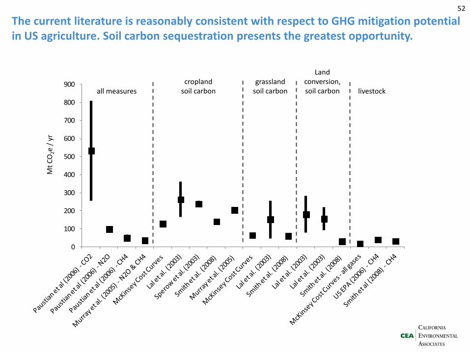
The current literature is reasonably consistent with respect to GHG mitigation potential in US agriculture. Soil carbon sequestration presents the greatest opportunity.
52
all measures cropland
soil carbon grassland
soil carbon
Land conversion, soil carbon livestock
Mt
CO
2e
/ yr
GHG Mitigation Executive summary > GHG emissions > GHG mitigation > Nitrogen pollution > Nitrogen mitigation
- Logic model - Literature review - Deep dive on croplands & grasslands - Livestock - Regional distribution - Economics
53
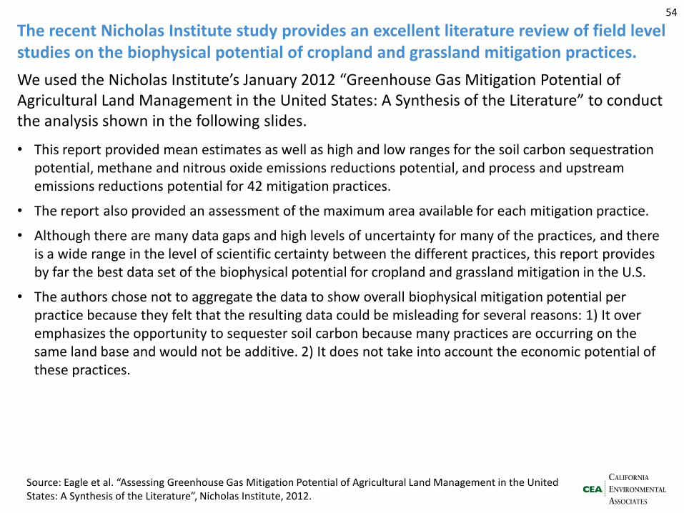
The recent Nicholas Institute study provides an excellent literature review of field level studies on the biophysical potential of cropland and grassland mitigation practices.
We used the Nicholas Institute’s January 2012 “Greenhouse Gas Mitigation Potential of Agricultural Land Management in the United States: A Synthesis of the Literature” to conduct the analysis shown in the following slides.
• This report provided mean estimates as well as high and low ranges for the soil carbon sequestration potential, methane and nitrous oxide emissions reductions potential, and process and upstream emissions reductions potential for 42 mitigation practices.
• The report also provided an assessment of the maximum area available for each mitigation practice.
• Although there are many data gaps and high levels of uncertainty for many of the practices, and there is a wide range in the level of scientific certainty between the different practices, this report provides by far the best data set of the biophysical potential for cropland and grassland mitigation in the U.S.
• The authors chose not to aggregate the data to show overall biophysical mitigation potential per practice because they felt that the resulting data could be misleading for several reasons: 1) It over emphasizes the opportunity to sequester soil carbon because many practices are occurring on the same land base and would not be additive. 2) It does not take into account the economic potential of these practices.
Source: Eagle et al. “Assessing Greenhouse Gas Mitigation Potential of Agricultural Land Management in the United States: A Synthesis of the Literature”, Nicholas Institute, 2012.
54
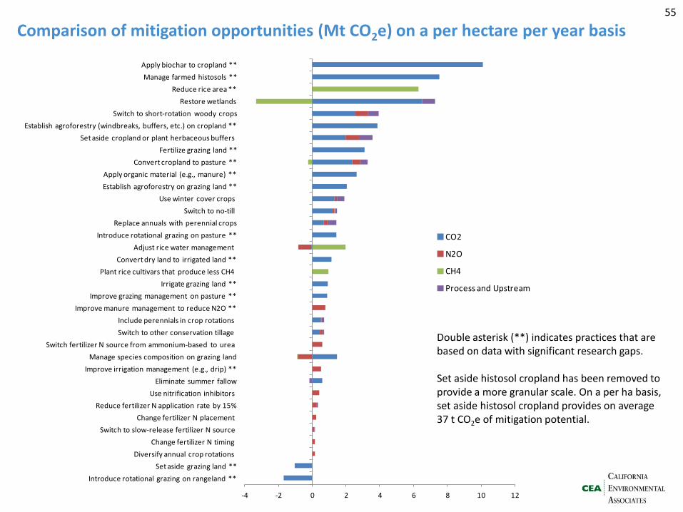
Comparison of mitigation opportunities (Mt CO2e) on a per hectare per year basis 55
-4 -2 0 2 4 6 8 10 12
Introduce rotational grazing on rangeland **
Set aside grazing land **
Diversify annual crop rotations
Change fertilizer N timing
Switch to slow-release fertilizer N source
Change fertilizer N placement
Reduce fertilizer N application rate by 15%
Use nitrification inhibitors
Eliminate summer fallow
Improve irrigation management (e.g., drip) **
Manage species composition on grazing land
Switch fertilizer N source from ammonium-based to urea
Switch to other conservation tillage
Include perennials in crop rotations
Improve manure management to reduce N2O **
Improve grazing management on pasture **
Irrigate grazing land **
Plant rice cultivars that produce less CH4
Convert dry land to irrigated land **
Adjust rice water management
Introduce rotational grazing on pasture **
Replace annuals with perennial crops
Switch to no-till
Use winter cover crops
Establish agroforestry on grazing land **
Apply organic material (e.g., manure) **
Convert cropland to pasture **
Fertilize grazing land **
Set aside cropland or plant herbaceous buffers
Establish agroforestry (windbreaks, buffers, etc.) on cropland **
Switch to short-rotation woody crops
Restore wetlands
Reduce rice area **
Manage farmed histosols **
Apply biochar to cropland **
GHG Mitigation Opportunity per Hectare (Mt CO2e)
CO2
N2O
CH4
Process and Upstream
Double asterisk (**) indicates practices that are based on data with significant research gaps. Set aside histosol cropland has been removed to provide a more granular scale. On a per ha basis, set aside histosol cropland provides on average 37 t CO2e of mitigation potential.
-4 -2 0 2 4 6 8 10 12
Introduce rotational grazing on rangeland **
Set aside grazing land **
Diversify annual crop rotations
Change fertilizer N timing
Switch to slow-release fertilizer N source
Change fertilizer N placement
Reduce fertilizer N application rate by 15%
Use nitrification inhibitors
Eliminate summer fallow
Improve irrigation management (e.g., drip) **
Manage species composition on grazing land
Switch fertilizer N source from ammonium-based to urea
Switch to other conservation tillage
Include perennials in crop rotations
Improve manure management to reduce N2O **
Improve grazing management on pasture **
Irrigate grazing land **
Plant rice cultivars that produce less CH4
Convert dry land to irrigated land **
Adjust rice water management
Introduce rotational grazing on pasture **
Replace annuals with perennial crops
Switch to no-till
Use winter cover crops
Establish agroforestry on grazing land **
Apply organic material (e.g., manure) **
Convert cropland to pasture **
Fertilize grazing land **
Set aside cropland or plant herbaceous buffers
Establish agroforestry (windbreaks, buffers, etc.) on cropland **
Switch to short-rotation woody crops
Restore wetlands
Reduce rice area **
Manage farmed histosols **
Apply biochar to cropland **
GHG Mitigation Opportunity per Hectare (Mt CO2e)
CO2
N2O
CH4
Process and Upstream
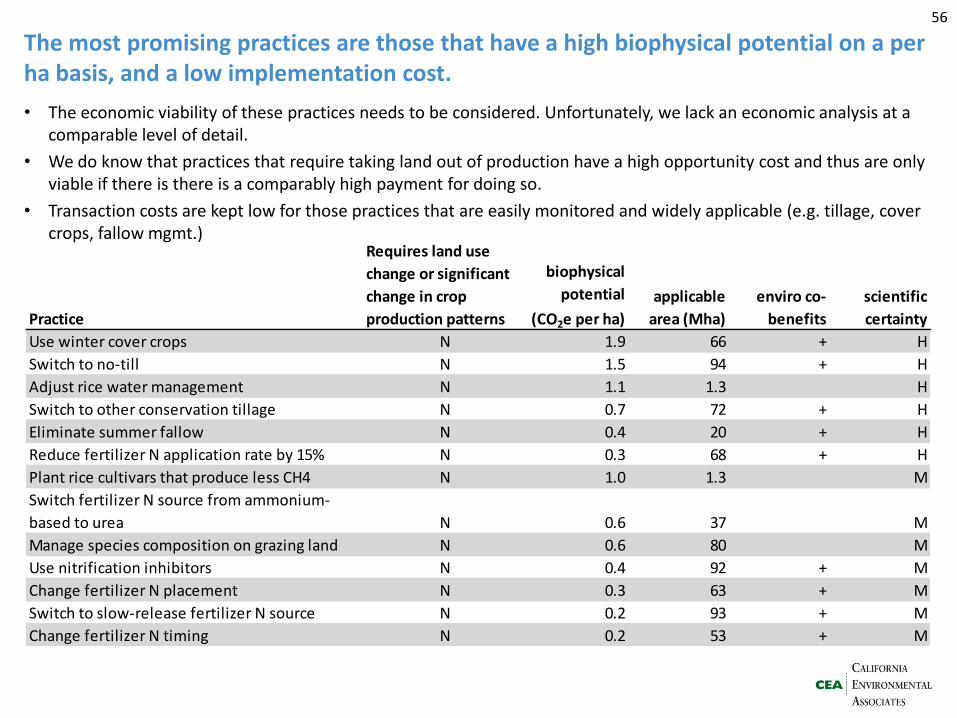
The most promising practices are those that have a high biophysical potential on a per ha basis, and a low implementation cost.
56
• The economic viability of these practices needs to be considered. Unfortunately, we lack an economic analysis at a comparable level of detail.
• We do know that practices that require taking land out of production have a high opportunity cost and thus are only viable if there is there is a comparably high payment for doing so.
• Transaction costs are kept low for those practices that are easily monitored and widely applicable (e.g. tillage, cover crops, fallow mgmt.)
Practice
Requires land use
change or significant
change in crop
production patterns
biophysical
potential
(CO2e per ha)
applicable
area (Mha)
enviro co-
benefits
scientific
certainty
Use winter cover crops N 1.9 66 + H
Switch to no-till N 1.5 94 + H
Adjust rice water management N 1.1 1.3 H
Switch to other conservation tillage N 0.7 72 + H
Eliminate summer fallow N 0.4 20 + H
Reduce fertilizer N application rate by 15% N 0.3 68 + H
Plant rice cultivars that produce less CH4 N 1.0 1.3 M
Switch fertilizer N source from ammonium-
based to urea N 0.6 37 M
Manage species composition on grazing land N 0.6 80 M
Use nitrification inhibitors N 0.4 92 + M
Change fertilizer N placement N 0.3 63 + M
Switch to slow-release fertilizer N source N 0.2 93 + M
Change fertilizer N timing N 0.2 53 + M
Practice
Requires land use
change or significant
change in crop
production patterns
biophysical
potential
(CO2e per ha)
applicable
area (Mha)
enviro co-
benefits
scientific
certainty
Establish agroforestry (windbreaks, buffers, etc.) on cropland partial 3.9 21 + L
Switch to short-rotation woody crops Y 3.9 40 + H
Set aside cropland or plant herbaceous buffers Y 3.6 17 + H
Convert cropland to pasture Y 3.1 unknown + H
Include perennials in crop rotations Y 0.7 56 + H
Diversify annual crop rotations Y 0.2 46 + H
Set aside histosol cropland Y 37.8 0.8 + L
Reduce rice area Y 6.3 1.3 L
Set aside grazing land Y -1.0 unknown + L
Restore wetlands Y 3.9 3.8 + M
Replace annuals with perennial crops Y 1.4 13 + M
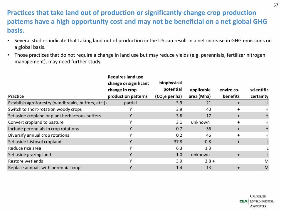
Practices that take land out of production or significantly change crop production patterns have a high opportunity cost and may not be beneficial on a net global GHG basis.
57
• Several studies indicate that taking land out of production in the US can result in a net increase in GHG emissions on a global basis.
• Those practices that do not require a change in land use but may reduce yields (e.g. perennials, fertilizer nitrogen management), may need further study.
58
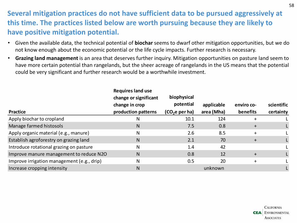
Several mitigation practices do not have sufficient data to be pursued aggressively at this time. The practices listed below are worth pursuing because they are likely to have positive mitigation potential.
Practice
Requires land use
change or significant
change in crop
production patterns
biophysical
potential
(CO2e per ha)
applicable
area (Mha)
enviro co-
benefits
scientific
certainty
Apply biochar to cropland N 10.1 124 + L
Manage farmed histosols N 7.5 0.8 + L
Apply organic material (e.g., manure) N 2.6 8.5 + L
Establish agroforestry on grazing land N 2.1 70 + L
Introduce rotational grazing on pasture N 1.4 42 L
Improve manure management to reduce N2O N 0.8 12 + L
Improve irrigation management (e.g., drip) N 0.5 20 + L
Increase cropping intensity N unknown L
• Given the available data, the technical potential of biochar seems to dwarf other mitigation opportunities, but we do not know enough about the economic potential or the life cycle impacts. Further research is necessary.
• Grazing land management is an area that deserves further inquiry. Mitigation opportunities on pasture land seem to have more certain potential than rangelands, but the sheer acreage of rangelands in the US means that the potential could be very significant and further research would be a worthwhile investment.
High level takeaways from Nicholas Institute’s assessment
Soil carbon sequestration provides a bigger opportunity than reduction of N2O or CH4. • Understanding the aggregate mitigation opportunity for soil carbon is challenging because the ability of any single
hectare of cropland to sequester soil is limited, and only 1 or 2 practices can be applied at one time. Adding the potential of all of these practices together is counting the same carbon multiple times.
• The additionality, reversibility, and additive (i.e. time limited) characteristics of soil carbon sequestration need to be considered.
• Because soil carbon sequestration opportunities are largely diffuse, they may be costly to implement.
• The soil sequestration potential of both biochar and grazing lands may be very large and should be studied further.
The impact of mitigation practices on commodity markets needs to be carefully considered. • Baker et al. 2011 finds that “climate mitigation opportunities increase the demand for land for nonfood benefits,
reduce commodity supply, and result in significant commodity market impacts.”
• Recent studies from both Iowa State University (Elobeid et al. 2011) and the Nicholas Institute (Mosnier et al. 2012) find that taking land out of food production in the US, either for biofuel production or afforestation, can lead to a net rise in global GHG emissions.
Nutrient use efficiency that is managed so as not to reduce yields is worth pursuing despite implementation barriers. It has potential to be a low cost, scientifically valid, widely applicable opportunity with significant environmental co-benefits.
Mitigation opportunities that are only applicable to very limited areas (e.g. rice, organic soils restoration, and wetlands restoration) may be low hanging fruit and worth pursuing, but will not have a significant impact in the aggregate.
59
GHG Mitigation Executive summary > GHG emissions > GHG mitigation > Nitrogen pollution > Nitrogen mitigation
- Logic model - Literature review - Deep dive on croplands & grasslands - Livestock - Regional distribution - Economics
60
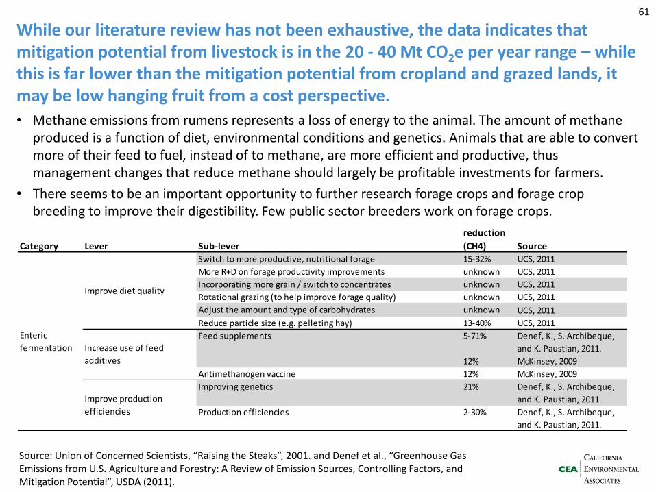
While our literature review has not been exhaustive, the data indicates that mitigation potential from livestock is in the 20 - 40 Mt CO2e per year range – while this is far lower than the mitigation potential from cropland and grazed lands, it may be low hanging fruit from a cost perspective.
• Methane emissions from rumens represents a loss of energy to the animal. The amount of methane produced is a function of diet, environmental conditions and genetics. Animals that are able to convert more of their feed to fuel, instead of to methane, are more efficient and productive, thus management changes that reduce methane should largely be profitable investments for farmers.
• There seems to be an important opportunity to further research forage crops and forage crop breeding to improve their digestibility. Few public sector breeders work on forage crops.
61
Source: Union of Concerned Scientists, “Raising the Steaks”, 2001. and Denef et al., “Greenhouse Gas Emissions from U.S. Agriculture and Forestry: A Review of Emission Sources, Controlling Factors, and Mitigation Potential”, USDA (2011).
Category Lever Sub-lever
%
reduction
(CH4) Source
Switch to more productive, nutritional forage 15-32% UCS, 2011
More R+D on forage productivity improvements unknown UCS, 2011
Incorporating more grain / switch to concentrates unknown UCS, 2011
Rotational grazing (to help improve forage quality) unknown UCS, 2011
Adjust the amount and type of carbohydrates unknown UCS, 2011
Reduce particle size (e.g. pelleting hay) 13-40% UCS, 2011
5-71% Denef, K., S. Archibeque,
and K. Paustian, 2011.
12% McKinsey, 2009
Antimethanogen vaccine 12% McKinsey, 2009
Improving genetics 21% Denef, K., S. Archibeque,
and K. Paustian, 2011.
Production efficiencies 2-30% Denef, K., S. Archibeque,
and K. Paustian, 2011.
Enteric
fermentation
Improve diet quality
Increase use of feed
additives
Improve production
efficiencies
Feed supplements
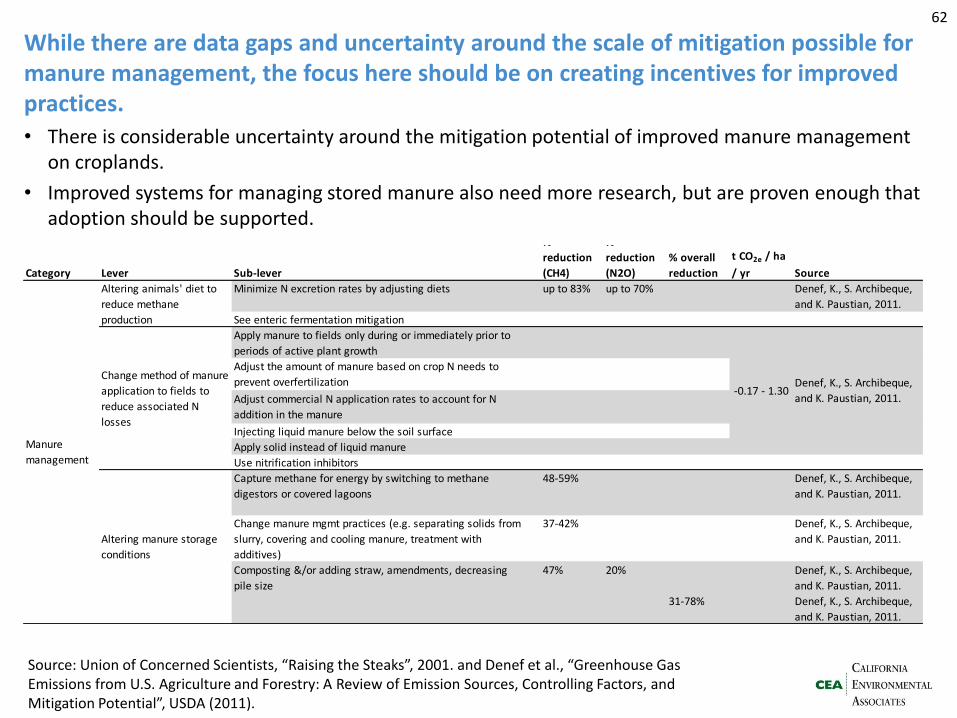
While there are data gaps and uncertainty around the scale of mitigation possible for manure management, the focus here should be on creating incentives for improved practices.
• There is considerable uncertainty around the mitigation potential of improved manure management on croplands.
• Improved systems for managing stored manure also need more research, but are proven enough that adoption should be supported.
62
Source: Union of Concerned Scientists, “Raising the Steaks”, 2001. and Denef et al., “Greenhouse Gas Emissions from U.S. Agriculture and Forestry: A Review of Emission Sources, Controlling Factors, and Mitigation Potential”, USDA (2011).
Category Lever Sub-lever
%
reduction
(CH4)
%
reduction
(N2O)
% overall
reduction
t CO2e / ha
/ yr Source
Minimize N excretion rates by adjusting diets up to 83% up to 70% Denef, K., S. Archibeque,
and K. Paustian, 2011.
See enteric fermentation mitigation
Apply manure to fields only during or immediately prior to
periods of active plant growth
Adjust the amount of manure based on crop N needs to
prevent overfertilization
Adjust commercial N application rates to account for N
addition in the manure
Injecting liquid manure below the soil surface
Apply solid instead of liquid manure
Use nitrification inhibitors
48-59% Denef, K., S. Archibeque,
and K. Paustian, 2011.
Change manure mgmt practices (e.g. separating solids from
slurry, covering and cooling manure, treatment with
additives)
37-42% Denef, K., S. Archibeque,
and K. Paustian, 2011.
47% 20% Denef, K., S. Archibeque,
and K. Paustian, 2011.
31-78% Denef, K., S. Archibeque,
and K. Paustian, 2011.
Denef, K., S. Archibeque,
and K. Paustian, 2011.
Capture methane for energy by switching to methane
digestors or covered lagoons
Composting &/or adding straw, amendments, decreasing
pile size
-0.17 - 1.30
Manure
management
Altering animals' diet to
reduce methane
production
Change method of manure
application to fields to
reduce associated N
losses
Altering manure storage
conditions
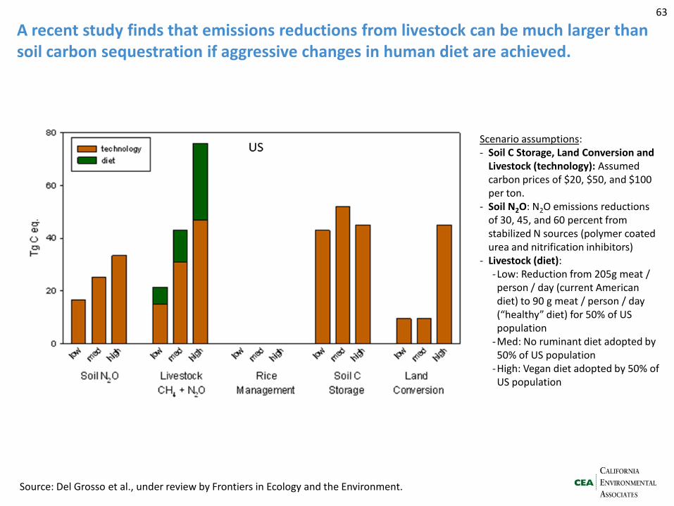
A recent study finds that emissions reductions from livestock can be much larger than soil carbon sequestration if aggressive changes in human diet are achieved.
63
Source: Del Grosso et al., under review by Frontiers in Ecology and the Environment.
Scenario assumptions: - Soil C Storage, Land Conversion and
Livestock (technology): Assumed carbon prices of $20, $50, and $100 per ton.
- Soil N2O: N2O emissions reductions of 30, 45, and 60 percent from stabilized N sources (polymer coated urea and nitrification inhibitors)
- Livestock (diet): - Low: Reduction from 205g meat / person / day (current American diet) to 90 g meat / person / day (“healthy” diet) for 50% of US population
-Med: No ruminant diet adopted by 50% of US population
-High: Vegan diet adopted by 50% of US population
GHG Mitigation Executive summary > GHG emissions > GHG mitigation > Nitrogen pollution > Nitrogen mitigation
- Logic model - Literature review - Deep dive on croplands & grasslands - Livestock - Regional distribution - Economics
64
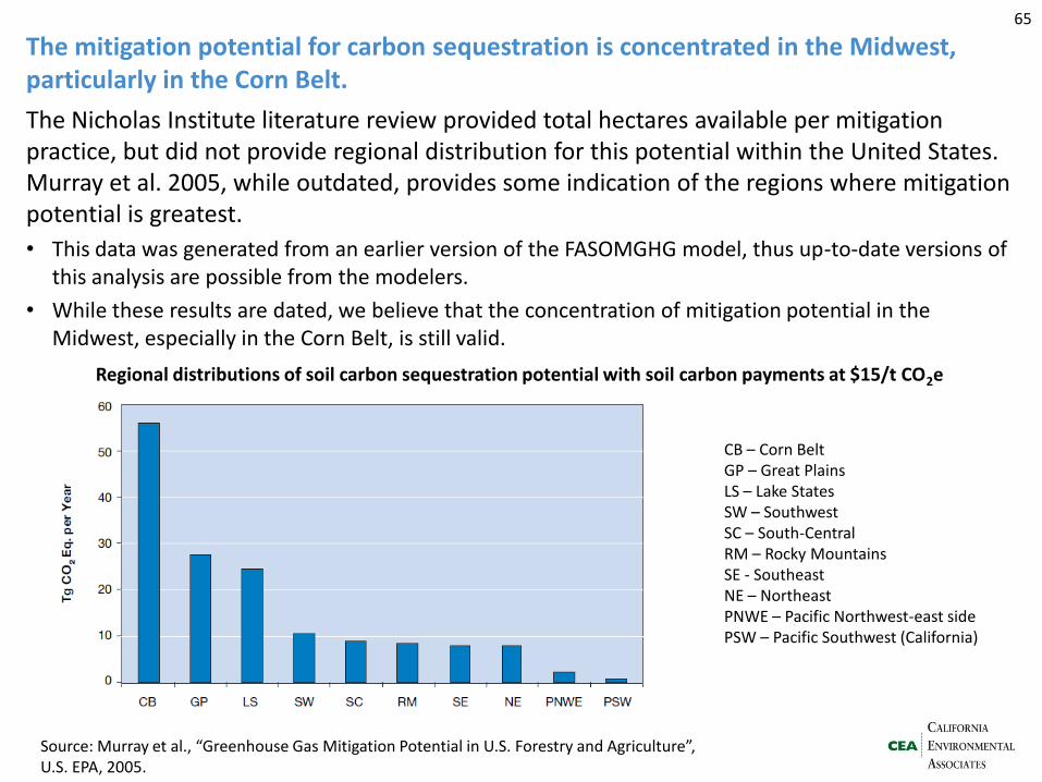
The mitigation potential for carbon sequestration is concentrated in the Midwest, particularly in the Corn Belt.
The Nicholas Institute literature review provided total hectares available per mitigation practice, but did not provide regional distribution for this potential within the United States. Murray et al. 2005, while outdated, provides some indication of the regions where mitigation potential is greatest.
• This data was generated from an earlier version of the FASOMGHG model, thus up-to-date versions of this analysis are possible from the modelers.
• While these results are dated, we believe that the concentration of mitigation potential in the Midwest, especially in the Corn Belt, is still valid.
65
CB – Corn Belt GP – Great Plains LS – Lake States SW – Southwest SC – South-Central RM – Rocky Mountains SE - Southeast NE – Northeast PNWE – Pacific Northwest-east side PSW – Pacific Southwest (California)
Regional distributions of soil carbon sequestration potential with soil carbon payments at $15/t CO2e
Source: Murray et al., “Greenhouse Gas Mitigation Potential in U.S. Forestry and Agriculture”, U.S. EPA, 2005.
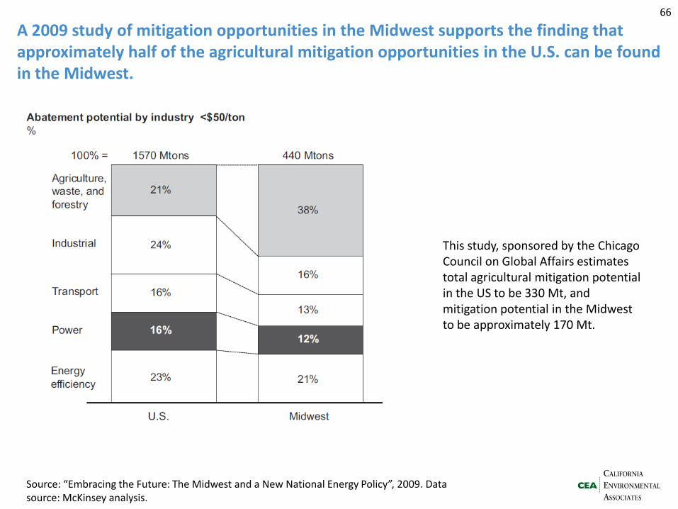
A 2009 study of mitigation opportunities in the Midwest supports the finding that approximately half of the agricultural mitigation opportunities in the U.S. can be found in the Midwest.
66
This study, sponsored by the Chicago Council on Global Affairs estimates total agricultural mitigation potential in the US to be 330 Mt, and mitigation potential in the Midwest to be approximately 170 Mt.
Source: “Embracing the Future: The Midwest and a New National Energy Policy”, 2009. Data source: McKinsey analysis.
GHG Mitigation Executive summary > GHG emissions > GHG mitigation > Nitrogen pollution > Nitrogen mitigation
- Logic model - Literature review - Deep dive on croplands & grasslands - Livestock - Regional distribution - Economics
67
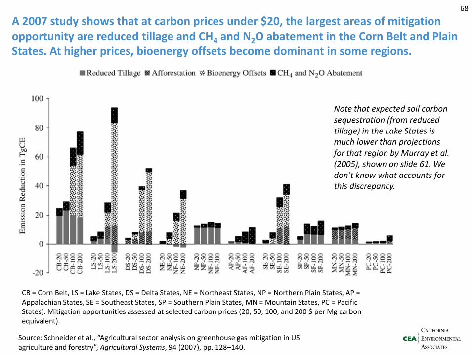
A 2007 study shows that at carbon prices under $20, the largest areas of mitigation opportunity are reduced tillage and CH4 and N2O abatement in the Corn Belt and Plain States. At higher prices, bioenergy offsets become dominant in some regions.
68
Source: Schneider et al., “Agricultural sector analysis on greenhouse gas mitigation in US agriculture and forestry”, Agricultural Systems, 94 (2007), pp. 128–140.
CB = Corn Belt, LS = Lake States, DS = Delta States, NE = Northeast States, NP = Northern Plain States, AP = Appalachian States, SE = Southeast States, SP = Southern Plain States, MN = Mountain States, PC = Pacific States). Mitigation opportunities assessed at selected carbon prices (20, 50, 100, and 200 $ per Mg carbon equivalent).
Note that expected soil carbon sequestration (from reduced tillage) in the Lake States is much lower than projections for that region by Murray et al. (2005), shown on slide 61. We don’t know what accounts for this discrepancy.
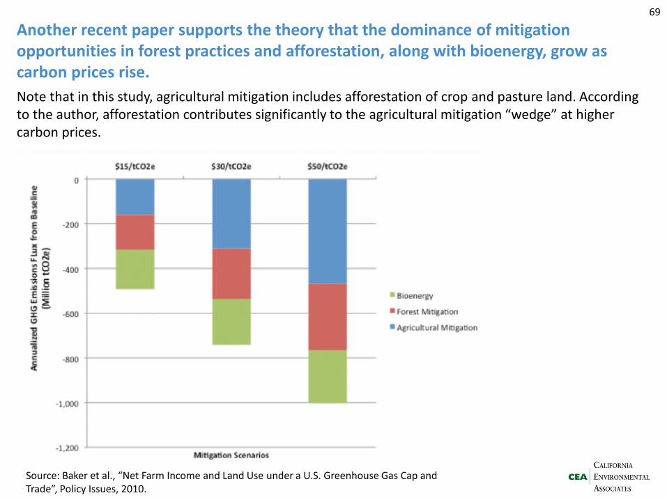
Another recent paper supports the theory that the dominance of mitigation opportunities in forest practices and afforestation, along with bioenergy, grow as carbon prices rise.
69
Note that in this study, agricultural mitigation includes afforestation of crop and pasture land. According to the author, afforestation contributes significantly to the agricultural mitigation “wedge” at higher carbon prices.
Source: Baker et al., “Net Farm Income and Land Use under a U.S. Greenhouse Gas Cap and Trade”, Policy Issues, 2010.
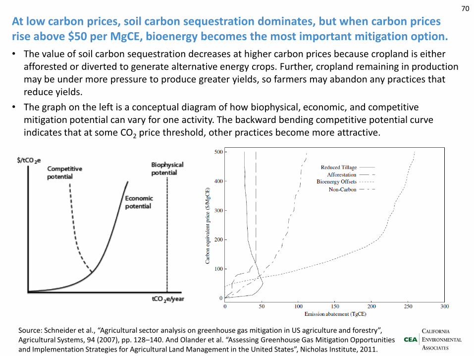
At low carbon prices, soil carbon sequestration dominates, but when carbon prices rise above $50 per MgCE, bioenergy becomes the most important mitigation option.
• The value of soil carbon sequestration decreases at higher carbon prices because cropland is either afforested or diverted to generate alternative energy crops. Further, cropland remaining in production may be under more pressure to produce greater yields, so farmers may abandon any practices that reduce yields.
• The graph on the left is a conceptual diagram of how biophysical, economic, and competitive mitigation potential can vary for one activity. The backward bending competitive potential curve indicates that at some CO2 price threshold, other practices become more attractive.
70
Source: Schneider et al., “Agricultural sector analysis on greenhouse gas mitigation in US agriculture and forestry”, Agricultural Systems, 94 (2007), pp. 128–140. And Olander et al. “Assessing Greenhouse Gas Mitigation Opportunities and Implementation Strategies for Agricultural Land Management in the United States”, Nicholas Institute, 2011.
Nitrogen pollution Executive summary > GHG emissions > GHG mitigation > Nitrogen pollution > Nitrogen mitigation
- Inputs and projections - Outputs
71
Section summary: Agricultural nitrogen is a major contributor to greenhouse gas pollution as well as air and water pollution. Agricultural nitrogen is growing, slowly. Corn and soybeans are the major contributors.
• Agricultural nitrogen – from synthetic fertilizer and crop biological fixation – is the greatest source of new reactive nitrogen in the US annually. Together, these sources of nitrogen are growing at ~1.5% / year.
• Fertilizer use has leveled off substantially from the growth years of the 1960s and 1970s. Mandates for biofuels will increase nitrogen fertilizer use, but not dramatically.
• Nitrogen losses to the atmosphere (as N2O, NOX, and NH3) and to aquatic systems are major sources of air pollution, greenhouse gas pollution, and water pollution. Unfortunately, the pathways of agricultural nitrogen are very difficult to track and measure, but literature suggests that as much as 20-30% ends up in aquatic systems.
• Corn is by far the largest user of nitrogen fertilizer of the major crops in the US, receiving over 40% of all applied nitrogen fertilizer. Corn is also the major crop least in compliance with best management practices (BMPs) for nutrient management.
72
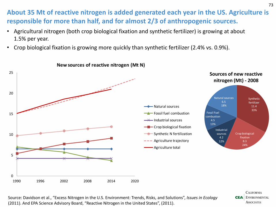
About 35 Mt of reactive nitrogen is added generated each year in the US. Agriculture is responsible for more than half, and for almost 2/3 of anthropogenic sources.
Source: Davidson et al., “Excess Nitrogen in the U.S. Environment: Trends, Risks, and Solutions”, Issues in Ecology (2011). And EPA Science Advisory Board, “Reactive Nitrogen in the United States”, (2011).
73
• Agricultural nitrogen (both crop biological fixation and synthetic fertilizer) is growing at about 1.5% per year.
• Crop biological fixation is growing more quickly than synthetic fertilizer (2.4% vs. 0.9%).
Synthetic
fertilizer11.433%
Crop biological
fixation8.324%
Industrial sources
4.212%
Fossil Fuel
combustion 4.5
13%
Natural sources6.518%
Sources of new reactive nitrogen (Mt) - 2008
0
5
10
15
20
25
1990 1996 2002 2008 2014 2020
New sources of reactive nitrogen (Mt N)
Natural sources
Fossil fuel combustion
Industrial sources
Crop biological fixation
Synthetic N fertilization
Agriculture trajectory
Agriculture total
0
2,000
4,000
6,000
8,000
10,000
12,000
14,000
1960
1962
1964
1966
1968
1970
1972
1974
1976
1978
1980
1982
1984
1986
1988
1990
1992
1994
1996
1998
2000
2002
2004
2006
2008
Nutrient use on US agricultural lands 1960 – 2009 (1,000 tons)
Nitrogen (N)
Phosphate (P2O5)
Potash (K2O)
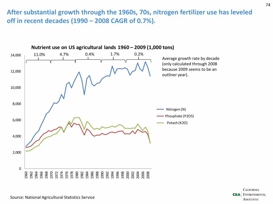
After substantial growth through the 1960s, 70s, nitrogen fertilizer use has leveled off in recent decades (1990 – 2008 CAGR of 0.7%).
74
Source: National Agricultural Statistics Service
0.2% 1.7% 0.4% 4.7% 11.0% Average growth rate by decade (only calculated through 2008 because 2009 seems to be an outliner year).
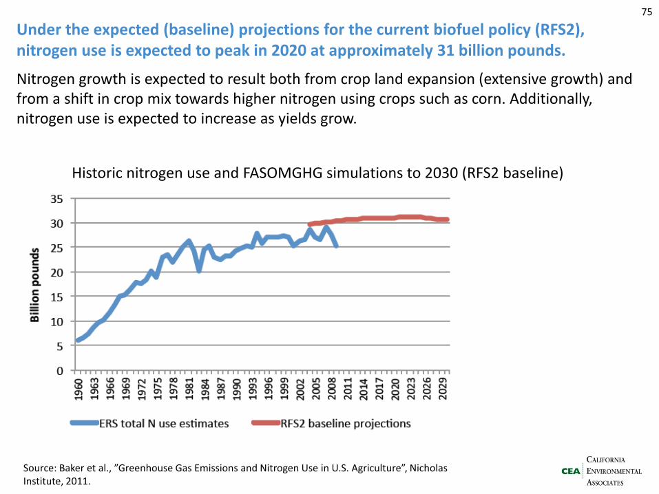
Under the expected (baseline) projections for the current biofuel policy (RFS2), nitrogen use is expected to peak in 2020 at approximately 31 billion pounds.
75
Source: Baker et al., ”Greenhouse Gas Emissions and Nitrogen Use in U.S. Agriculture”, Nicholas Institute, 2011.
Nitrogen growth is expected to result both from crop land expansion (extensive growth) and from a shift in crop mix towards higher nitrogen using crops such as corn. Additionally, nitrogen use is expected to increase as yields grow.
Historic nitrogen use and FASOMGHG simulations to 2030 (RFS2 baseline)
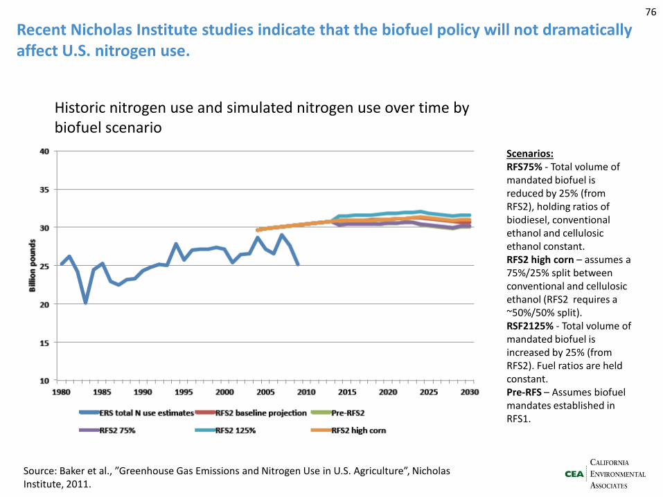
Recent Nicholas Institute studies indicate that the biofuel policy will not dramatically affect U.S. nitrogen use.
76
Source: Baker et al., ”Greenhouse Gas Emissions and Nitrogen Use in U.S. Agriculture”, Nicholas Institute, 2011.
Historic nitrogen use and simulated nitrogen use over time by biofuel scenario
Scenarios: RFS75% - Total volume of mandated biofuel is reduced by 25% (from RFS2), holding ratios of biodiesel, conventional ethanol and cellulosic ethanol constant. RFS2 high corn – assumes a 75%/25% split between conventional and cellulosic ethanol (RFS2 requires a ~50%/50% split). RSF2125% - Total volume of mandated biofuel is increased by 25% (from RFS2). Fuel ratios are held constant. Pre-RFS – Assumes biofuel mandates established in RFS1.
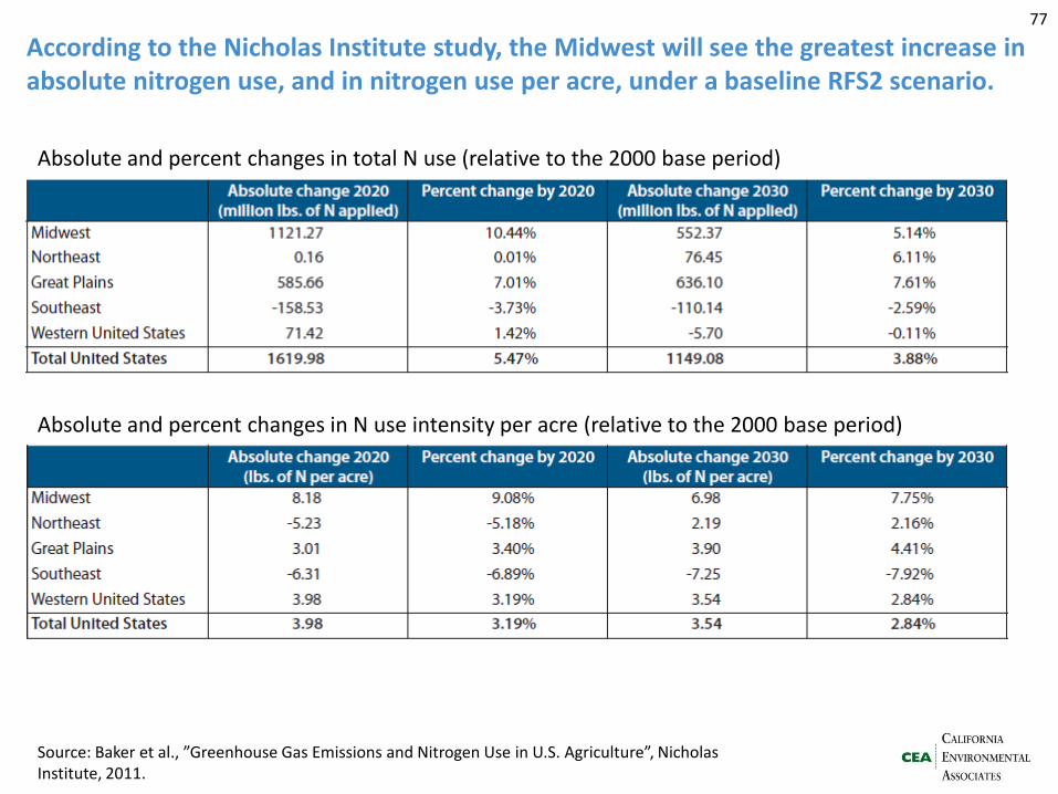
According to the Nicholas Institute study, the Midwest will see the greatest increase in absolute nitrogen use, and in nitrogen use per acre, under a baseline RFS2 scenario.
77
Absolute and percent changes in total N use (relative to the 2000 base period)
Absolute and percent changes in N use intensity per acre (relative to the 2000 base period)
Source: Baker et al., ”Greenhouse Gas Emissions and Nitrogen Use in U.S. Agriculture”, Nicholas Institute, 2011.
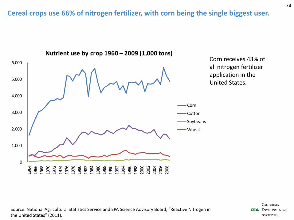
Cereal crops use 66% of nitrogen fertilizer, with corn being the single biggest user. 78
Source: National Agricultural Statistics Service and EPA Science Advisory Board, “Reactive Nitrogen in the United States” (2011).
0
1,000
2,000
3,000
4,000
5,000
6,000
1964
1966
1968
1970
1972
1974
1976
1978
1980
1982
1984
1986
1988
1990
1992
1994
1996
1998
2000
2002
2004
2006
2008
Nutrient use by crop 1960 – 2009 (1,000 tons)
Corn
Cotton
Soybeans
Wheat
Corn receives 43% of all nitrogen fertilizer application in the United States.
0
50
100
150
200
250
300
350
Kg N applied per hectare
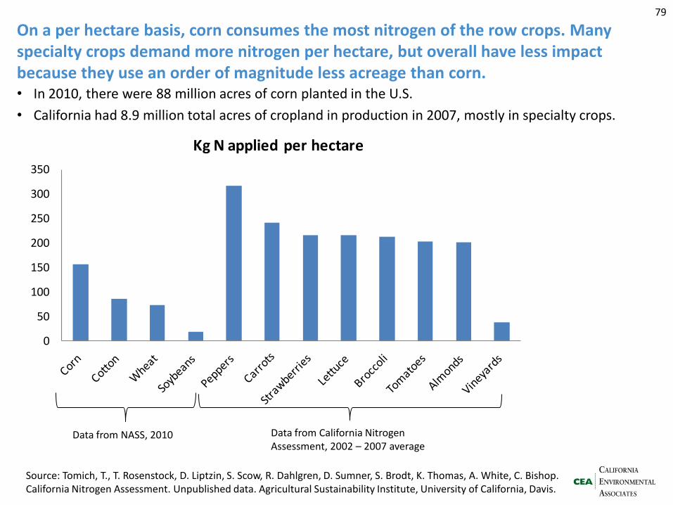
On a per hectare basis, corn consumes the most nitrogen of the row crops. Many specialty crops demand more nitrogen per hectare, but overall have less impact because they use an order of magnitude less acreage than corn. • In 2010, there were 88 million acres of corn planted in the U.S.
• California had 8.9 million total acres of cropland in production in 2007, mostly in specialty crops.
79
Data from NASS, 2010 Data from California Nitrogen Assessment, 2002 – 2007 average
Source: Tomich, T., T. Rosenstock, D. Liptzin, S. Scow, R. Dahlgren, D. Sumner, S. Brodt, K. Thomas, A. White, C. Bishop. California Nitrogen Assessment. Unpublished data. Agricultural Sustainability Institute, University of California, Davis.
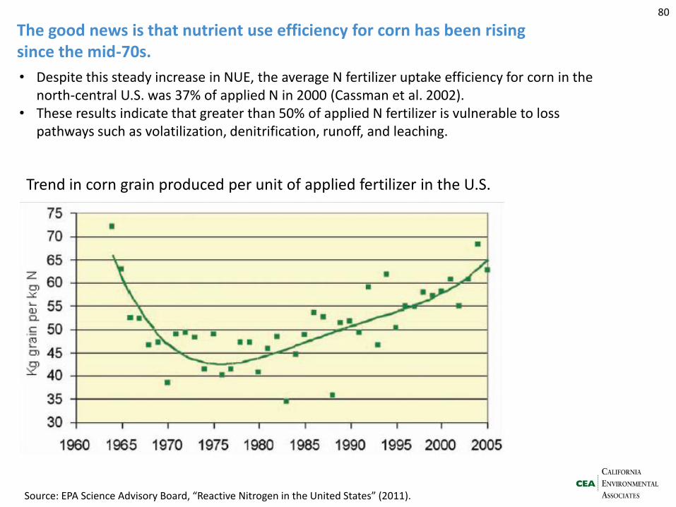
The good news is that nutrient use efficiency for corn has been rising since the mid-70s.
80
Trend in corn grain produced per unit of applied fertilizer in the U.S.
Source: EPA Science Advisory Board, “Reactive Nitrogen in the United States” (2011).
• Despite this steady increase in NUE, the average N fertilizer uptake efficiency for corn in the north-central U.S. was 37% of applied N in 2000 (Cassman et al. 2002).
• These results indicate that greater than 50% of applied N fertilizer is vulnerable to loss pathways such as volatilization, denitrification, runoff, and leaching.
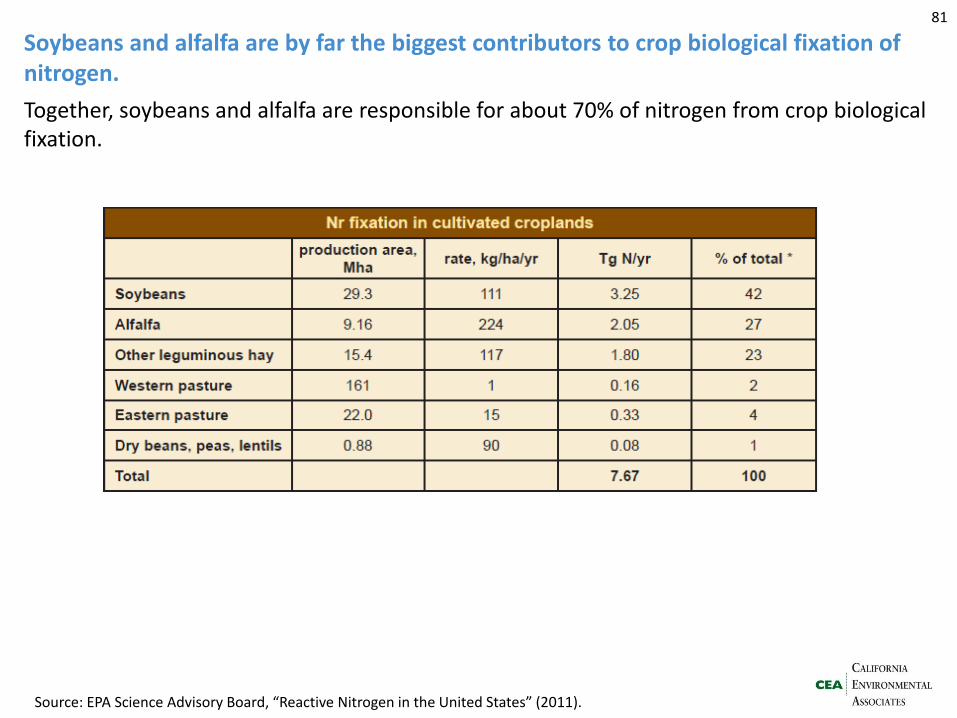
Soybeans and alfalfa are by far the biggest contributors to crop biological fixation of nitrogen.
Together, soybeans and alfalfa are responsible for about 70% of nitrogen from crop biological fixation.
81
Source: EPA Science Advisory Board, “Reactive Nitrogen in the United States” (2011).
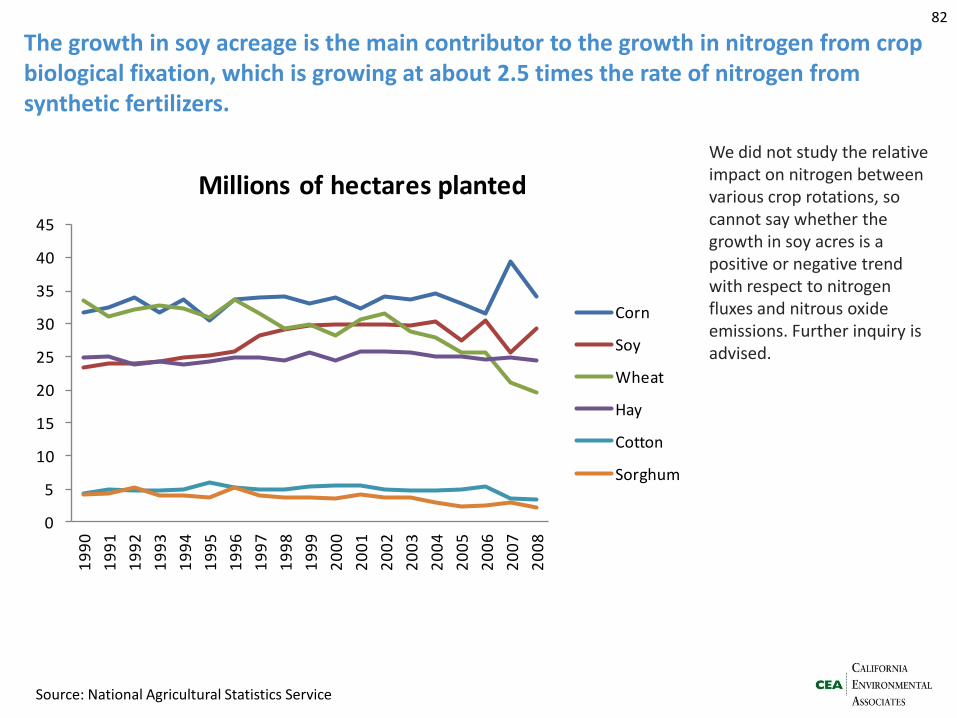
The growth in soy acreage is the main contributor to the growth in nitrogen from crop biological fixation, which is growing at about 2.5 times the rate of nitrogen from synthetic fertilizers.
82
0
5
10
15
20
25
30
35
40
45
19
90
19
91
19
92
19
93
19
94
19
95
19
96
19
97
19
98
19
99
20
00
20
01
20
02
20
03
20
04
20
05
20
06
20
07
20
08
Millions of hectares planted
Corn
Soy
Wheat
Hay
Cotton
Sorghum
Source: National Agricultural Statistics Service
We did not study the relative impact on nitrogen between various crop rotations, so cannot say whether the growth in soy acres is a positive or negative trend with respect to nitrogen fluxes and nitrous oxide emissions. Further inquiry is advised.
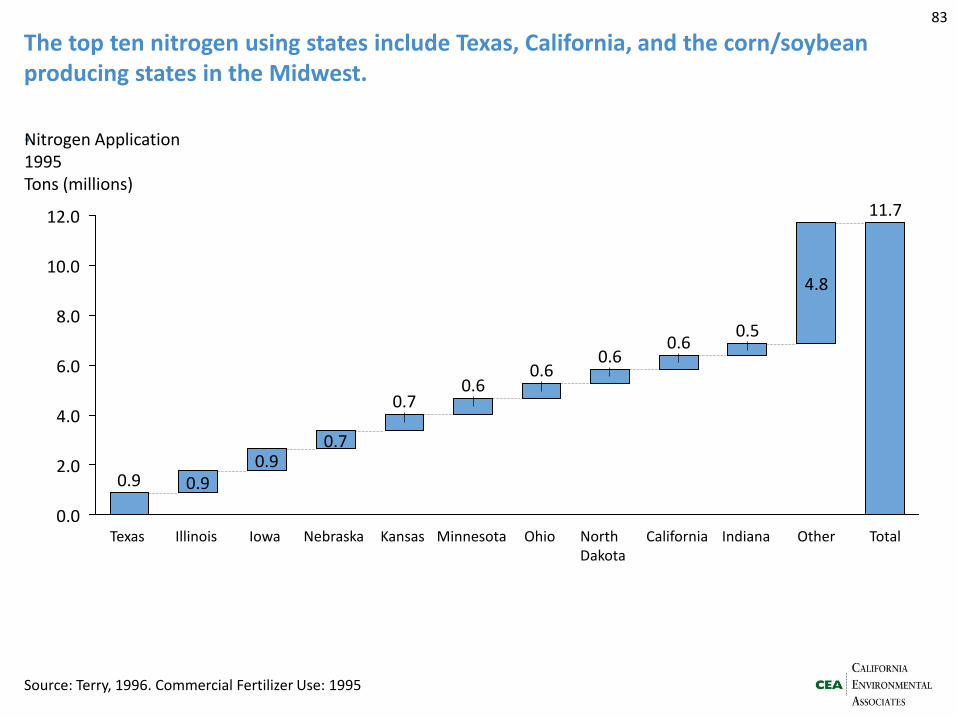
The top ten nitrogen using states include Texas, California, and the corn/soybean producing states in the Midwest. .
2.0
4.0
Indiana
4.8
Other
0.5
California
0.6
11.7
Total 0.0
North Dakota
0.6
Ohio
0.6
Minnesota
0.6
Kansas
0.7
Nebraska
0.7
Iowa
0.9
Illinois
0.9
Texas
0.9
6.0
8.0
10.0
12.0
Nitrogen Application 1995 Tons (millions)
Source: Terry, 1996. Commercial Fertilizer Use: 1995
83
Nitrogen pollution Executive summary > GHG emissions > GHG mitigation > Nitrogen pollution > Nitrogen mitigation
- Inputs and projections - Outputs
84
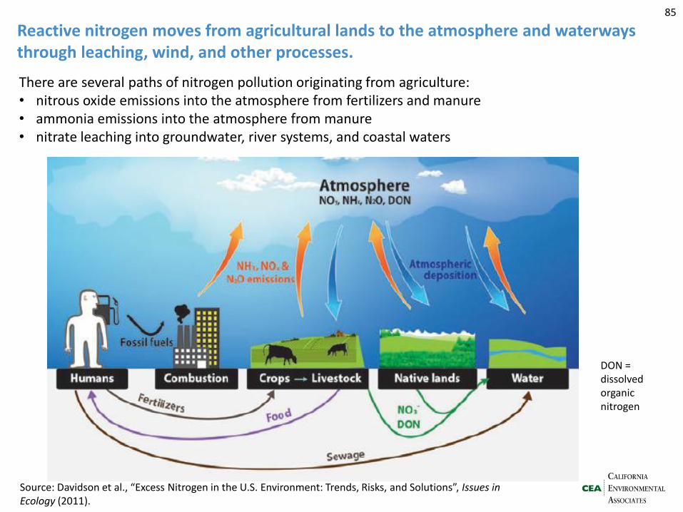
Reactive nitrogen moves from agricultural lands to the atmosphere and waterways through leaching, wind, and other processes.
There are several paths of nitrogen pollution originating from agriculture: • nitrous oxide emissions into the atmosphere from fertilizers and manure • ammonia emissions into the atmosphere from manure • nitrate leaching into groundwater, river systems, and coastal waters
85
Source: Davidson et al., “Excess Nitrogen in the U.S. Environment: Trends, Risks, and Solutions”, Issues in Ecology (2011).
DON = dissolved organic nitrogen
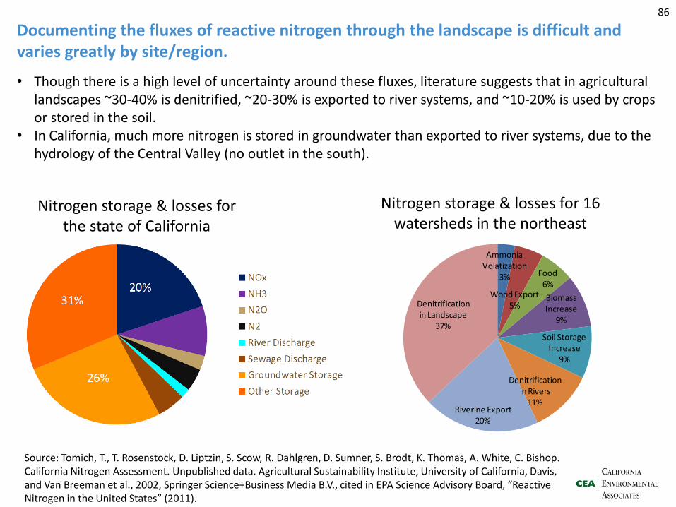
Documenting the fluxes of reactive nitrogen through the landscape is difficult and varies greatly by site/region.
• Though there is a high level of uncertainty around these fluxes, literature suggests that in agricultural landscapes ~30-40% is denitrified, ~20-30% is exported to river systems, and ~10-20% is used by crops or stored in the soil.
• In California, much more nitrogen is stored in groundwater than exported to river systems, due to the hydrology of the Central Valley (no outlet in the south).
86
Nitrogen storage & losses for 16 watersheds in the northeast
Nitrogen storage & losses for the state of California
Source: Tomich, T., T. Rosenstock, D. Liptzin, S. Scow, R. Dahlgren, D. Sumner, S. Brodt, K. Thomas, A. White, C. Bishop. California Nitrogen Assessment. Unpublished data. Agricultural Sustainability Institute, University of California, Davis, and Van Breeman et al., 2002, Springer Science+Business Media B.V., cited in EPA Science Advisory Board, “Reactive Nitrogen in the United States” (2011).
Ammonia Volatization
3%
Wood Export5%
Food6%
Biomass Increase
9%
Soil Storage Increase
9%
Denitrification in Rivers
11%Riverine Export
20%
Denitrification in Landscape
37%
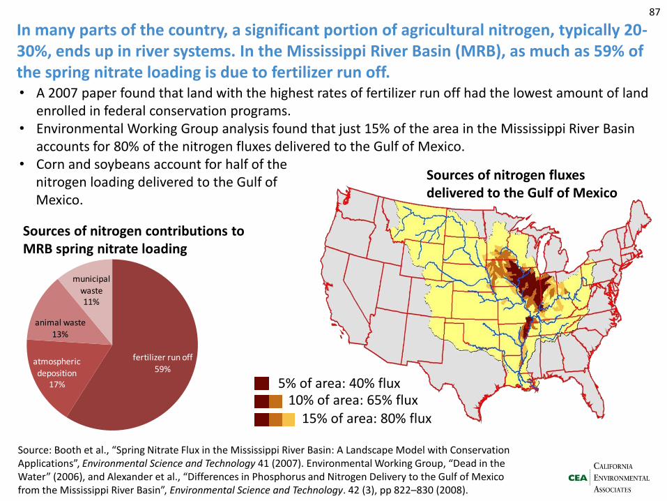
In many parts of the country, a significant portion of agricultural nitrogen, typically 20-30%, ends up in river systems. In the Mississippi River Basin (MRB), as much as 59% of the spring nitrate loading is due to fertilizer run off.
87
Source: Booth et al., “Spring Nitrate Flux in the Mississippi River Basin: A Landscape Model with Conservation Applications”, Environmental Science and Technology 41 (2007). Environmental Working Group, “Dead in the Water” (2006), and Alexander et al., “Differences in Phosphorus and Nitrogen Delivery to the Gulf of Mexico from the Mississippi River Basin”, Environmental Science and Technology. 42 (3), pp 822–830 (2008).
• A 2007 paper found that land with the highest rates of fertilizer run off had the lowest amount of land enrolled in federal conservation programs.
• Environmental Working Group analysis found that just 15% of the area in the Mississippi River Basin accounts for 80% of the nitrogen fluxes delivered to the Gulf of Mexico.
• Corn and soybeans account for half of the nitrogen loading delivered to the Gulf of Mexico.
15% of area: 80% flux 10% of area: 65% flux
5% of area: 40% flux
fertilizer run off
59%atmospheric deposition
17%
animal waste13%
municipal
waste 11%
Sources of nitrogen contributions to MRB spring nitrate loading
Sources of nitrogen fluxes delivered to the Gulf of Mexico
Nitrogen mitigation Executive summary > GHG emissions > GHG mitigation > Nitrogen pollution > Nitrogen mitigation
88
- Logic model - Diet and behavior - Best management
practices - Lessons from Europe
Section summary: Voluntary conservation measures in the U.S. are helping, but the European experience indicates that regulation is a much more powerful solution.
• USDA’s Conservation Effectiveness Assessment Program has found that in the Upper Mississippi River Basin, conservation practices adopted voluntarily between 2003 and 2006 have reduced nitrogen losses by about 20%. However, they also find that treating additional acreage could reduce nitrogen losses by an additional 40%.
• Analysis of losses along food supply chains indicate that diet choice matters a lot when it comes to nitrogen losses. Meat, especially beef, is a very inefficient user of nitrogen.
• The experience in Denmark and the Netherlands indicate that reducing nitrogen fertilizer can have a very significant impact on air quality and surface water quality. These countries reduced fertilizer use through regulation.
• The European experience is mixed, though. Historic data on the Thames River indicates that increases or decreases in nitrogen losses on agricultural lands can take a long time (decades) to impact on aquatic systems depending on the hydrology of the watershed.
• Because of the size and complexity of many of the river basis in the U.S., it may take a long time before the results of agricultural conservation measures can be observed in the aquatic systems.
89
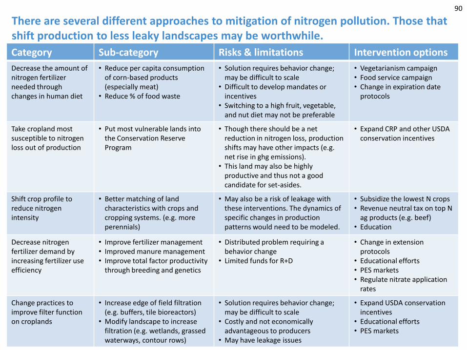
There are several different approaches to mitigation of nitrogen pollution. Those that shift production to less leaky landscapes may be worthwhile.
Category Sub-category Risks & limitations Intervention options
Decrease the amount of nitrogen fertilizer needed through changes in human diet
• Reduce per capita consumption of corn-based products (especially meat)
• Reduce % of food waste
• Solution requires behavior change; may be difficult to scale
• Difficult to develop mandates or incentives
• Switching to a high fruit, vegetable, and nut diet may not be preferable
• Vegetarianism campaign • Food service campaign • Change in expiration date
protocols
Take cropland most susceptible to nitrogen loss out of production
• Put most vulnerable lands into the Conservation Reserve Program
• Though there should be a net reduction in nitrogen loss, production shifts may have other impacts (e.g. net rise in ghg emissions).
• This land may also be highly productive and thus not a good candidate for set-asides.
• Expand CRP and other USDA conservation incentives
Shift crop profile to reduce nitrogen intensity
• Better matching of land characteristics with crops and cropping systems. (e.g. more perennials)
• May also be a risk of leakage with these interventions. The dynamics of specific changes in production patterns would need to be modeled.
• Subsidize the lowest N crops • Revenue neutral tax on top N
ag products (e.g. beef) • Education
Decrease nitrogen fertilizer demand by increasing fertilizer use efficiency
• Improve fertilizer management • Improved manure management • Improve total factor productivity
through breeding and genetics
• Distributed problem requiring a behavior change
• Limited funds for R+D
• Change in extension protocols
• Educational efforts • PES markets • Regulate nitrate application
rates
Change practices to improve filter function on croplands
• Increase edge of field filtration (e.g. buffers, tile bioreactors)
• Modify landscape to increase filtration (e.g. wetlands, grassed waterways, contour rows)
• Solution requires behavior change; may be difficult to scale
• Costly and not economically advantageous to producers
• May have leakage issues
• Expand USDA conservation incentives
• Educational efforts • PES markets
90

Nitrogen mitigation Executive summary > GHG emissions > GHG mitigation > Nitrogen pollution > Nitrogen mitigation
91
- Logic model - Diet and behavior - Best management
practices - Lessons from Europe
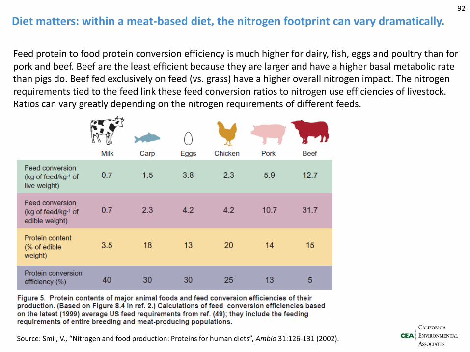
Diet matters: within a meat-based diet, the nitrogen footprint can vary dramatically. 92
Source: Smil, V., “Nitrogen and food production: Proteins for human diets”, Ambio 31:126-131 (2002).
Feed protein to food protein conversion efficiency is much higher for dairy, fish, eggs and poultry than for pork and beef. Beef are the least efficient because they are larger and have a higher basal metabolic rate than pigs do. Beef fed exclusively on feed (vs. grass) have a higher overall nitrogen impact. The nitrogen requirements tied to the feed link these feed conversion ratios to nitrogen use efficiencies of livestock. Ratios can vary greatly depending on the nitrogen requirements of different feeds.
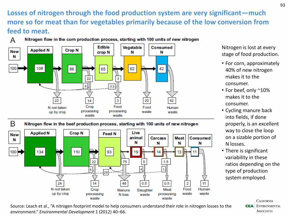
Losses of nitrogen through the food production system are very significant—much more so for meat than for vegetables primarily because of the low conversion from feed to meat.
93
Source: Leach et al., “A nitrogen footprint model to help consumers understand their role in nitrogen losses to the environment.” Environmental Development 1 (2012) 40–66.
Nitrogen is lost at every stage of food production.
• For corn, approximately 40% of new nitrogen makes it to the consumer.
• For beef, only ~10% makes it to the consumer.
• Cycling manure back into fields, if done properly, is an excellent way to close the loop on a sizable portion of N losses.
• There is significant variability in these ratios depending on the type of production system employed.
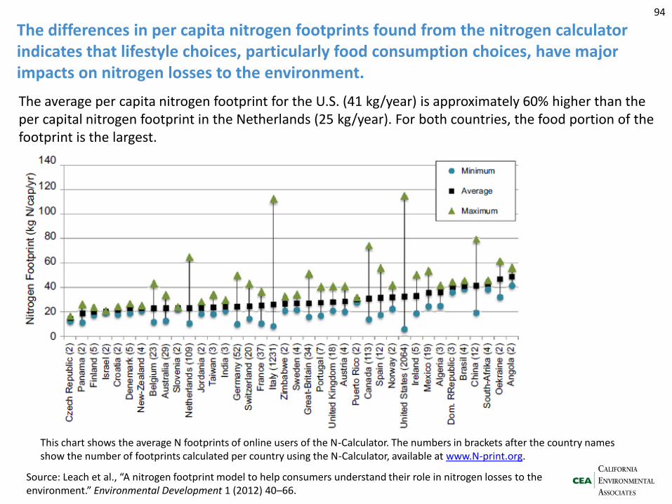
The differences in per capita nitrogen footprints found from the nitrogen calculator indicates that lifestyle choices, particularly food consumption choices, have major impacts on nitrogen losses to the environment.
94
Source: Leach et al., “A nitrogen footprint model to help consumers understand their role in nitrogen losses to the environment.” Environmental Development 1 (2012) 40–66.
The average per capita nitrogen footprint for the U.S. (41 kg/year) is approximately 60% higher than the per capital nitrogen footprint in the Netherlands (25 kg/year). For both countries, the food portion of the footprint is the largest.
This chart shows the average N footprints of online users of the N-Calculator. The numbers in brackets after the country names show the number of footprints calculated per country using the N-Calculator, available at www.N-print.org.

Nitrogen mitigation Executive summary > GHG emissions > GHG mitigation > Nitrogen pollution > Nitrogen mitigation
95
- Logic model - Diet and behavior - Best management
practices - Lessons from Europe
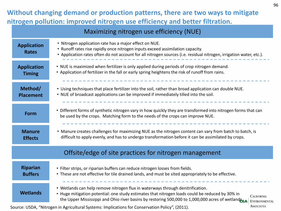
Application Rates
Application Timing
Method/ Placement
Form
Manure Effects
Maximizing nitrogen use efficiency (NUE)
• Nitrogen application rate has a major effect on NUE. • Runoff rates rise rapidly once nitrogen inputs exceed assimilation capacity. • Application rates often do not account for all nitrogen sources (i.e. residual nitrogen, irrigation water, etc.).
• NUE is maximized when fertilizer is only applied during periods of crop nitrogen demand. • Application of fertilizer in the fall or early spring heightens the risk of runoff from rains.
• Using techniques that place fertilizer into the soil, rather than broad application can double NUE. • NUE of broadcast applications can be improved if immediately tilled into the soil.
• Different forms of synthetic nitrogen vary in how quickly they are transformed into nitrogen forms that can be used by the crops. Matching form to the needs of the crops can improve NUE.
• Manure creates challenges for maximizing NUE as the nitrogen content can vary from batch to batch, is difficult to apply evenly, and has to undergo transformation before it can be assimilated by crops.
Source: USDA, “Nitrogen in Agricultural Systems: Implications for Conservation Policy”, (2011).
Riparian Buffers
Wetlands • Wetlands can help remove nitrogen flux in waterways through denitrification. • Huge mitigation potential: one study estimates that nitrogen loads could be reduced by 30% in
the Upper Mississippi and Ohio river basins by restoring 500,000 to 1,000,000 acres of wetlands
Offsite/edge of site practices for nitrogen management
• Filter strips, or riparian buffers can reduce nitrogen losses from fields. • These are not effective for tile drained lands, and must be sited appropriately to be effective.
96
Without changing demand or production patterns, there are two ways to mitigate nitrogen pollution: improved nitrogen use efficiency and better filtration.
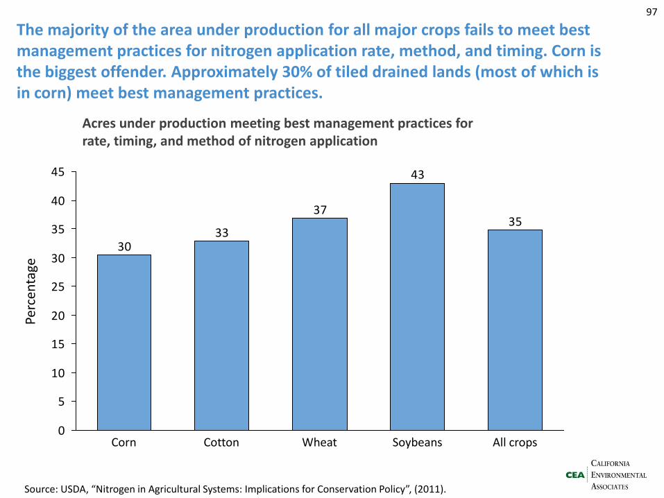
The majority of the area under production for all major crops fails to meet best management practices for nitrogen application rate, method, and timing. Corn is the biggest offender. Approximately 30% of tiled drained lands (most of which is in corn) meet best management practices.
43
37
3330
35
0
5
10
15
20
25
30
35
40
45
All crops Soybeans Corn Wheat Cotton
Source: USDA, “Nitrogen in Agricultural Systems: Implications for Conservation Policy”, (2011).
97
Acres under production meeting best management practices for rate, timing, and method of nitrogen application
Perc
enta
ge
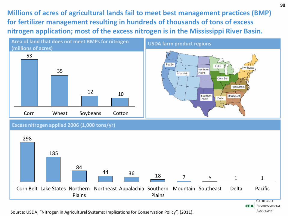
Millions of acres of agricultural lands fail to meet best management practices (BMP) for fertilizer management resulting in hundreds of thousands of tons of excess nitrogen application; most of the excess nitrogen is in the Mississippi River Basin.
Soybeans
12
Cotton
10
Wheat
35
Corn
53
Area of land that does not meet BMPs for nitrogen (millions of acres)
Excess nitrogen applied 2006 (1,000 tons/yr)
115718364484
185
298
Lake States Northern Plains
Corn Belt Northeast Southern Plains
Appalachia Mountain Pacific Delta Southeast
USDA farm product regions
Source: USDA, “Nitrogen in Agricultural Systems: Implications for Conservation Policy”, (2011).
98
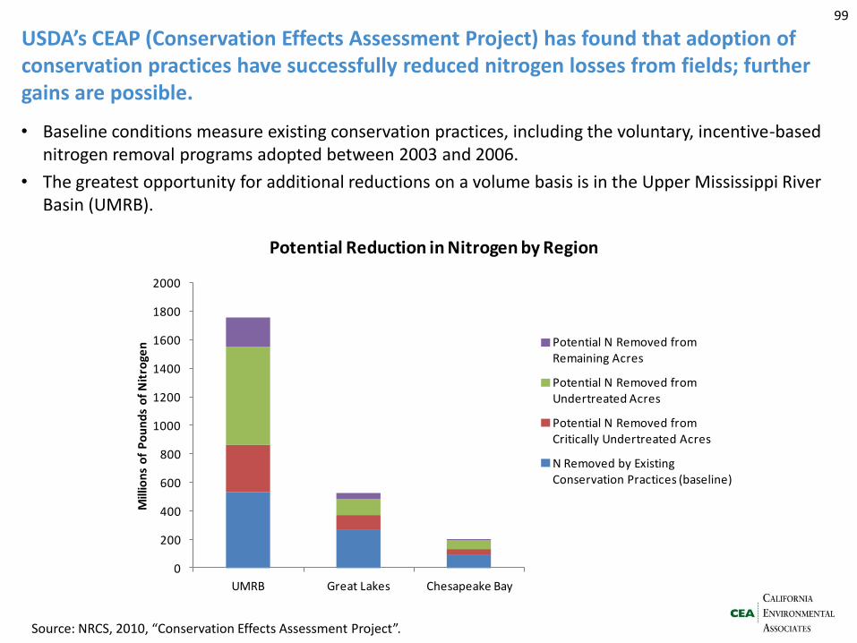
USDA’s CEAP (Conservation Effects Assessment Project) has found that adoption of conservation practices have successfully reduced nitrogen losses from fields; further gains are possible.
99
• Baseline conditions measure existing conservation practices, including the voluntary, incentive-based nitrogen removal programs adopted between 2003 and 2006.
• The greatest opportunity for additional reductions on a volume basis is in the Upper Mississippi River Basin (UMRB).
Source: NRCS, 2010, “Conservation Effects Assessment Project”.
0
200
400
600
800
1000
1200
1400
1600
1800
2000
UMRB Great Lakes Chesapeake Bay
Mill
ion
s o
f P
ou
nd
s o
f N
itro
gen
Potential Reduction in Nitrogen by Region
Potential N Removed from Remaining Acres
Potential N Removed from Undertreated Acres
Potential N Removed from Critically Undertreated Acres
N Removed by Existing Conservation Practices (baseline)
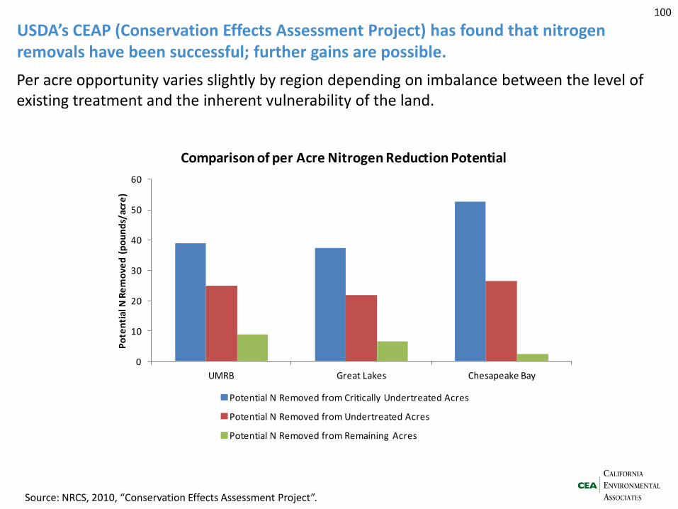
USDA’s CEAP (Conservation Effects Assessment Project) has found that nitrogen removals have been successful; further gains are possible.
100
Per acre opportunity varies slightly by region depending on imbalance between the level of existing treatment and the inherent vulnerability of the land.
Source: NRCS, 2010, “Conservation Effects Assessment Project”.
0
10
20
30
40
50
60
UMRB Great Lakes Chesapeake Bay
Po
ten
tial
N R
em
ove
d (
po
un
ds/
acre
)
Comparison of per Acre Nitrogen Reduction Potential
Potential N Removed from Critically Undertreated Acres
Potential N Removed from Undertreated Acres
Potential N Removed from Remaining Acres
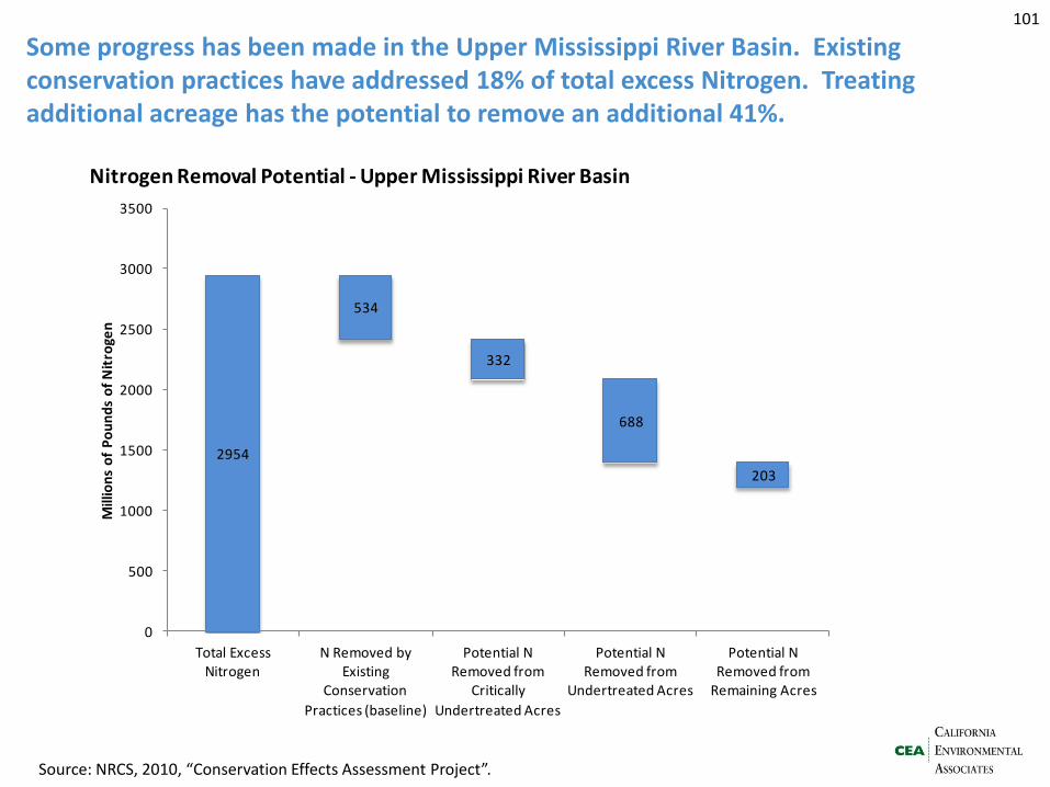
Some progress has been made in the Upper Mississippi River Basin. Existing conservation practices have addressed 18% of total excess Nitrogen. Treating additional acreage has the potential to remove an additional 41%.
101
Source: NRCS, 2010, “Conservation Effects Assessment Project”.
2954
534
332
688
203
0
500
1000
1500
2000
2500
3000
3500
Total Excess Nitrogen
N Removed by Existing
Conservation
Practices (baseline)
Potential N Removed from
Critically
Undertreated Acres
Potential N Removed from
Undertreated Acres
Potential N Removed from
Remaining Acres
Mill
ion
s o
f P
ou
nd
s o
f N
itro
gen
Nitrogen Removal Potential - Upper Mississippi River Basin
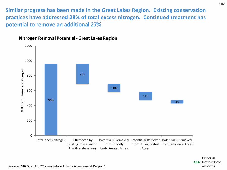
Similar progress has been made in the Great Lakes Region. Existing conservation practices have addressed 28% of total excess nitrogen. Continued treatment has potential to remove an additional 27%.
102
Source: NRCS, 2010, “Conservation Effects Assessment Project”.
956
265
106
110
45
0
200
400
600
800
1000
1200
Total Excess Nitrogen N Removed by Existing Conservation Practices (baseline)
Potential N Removed from Critically
Undertreated Acres
Potential N Removed from Undertreated
Acres
Potential N Removed from Remaining Acres
Mill
ion
s o
f P
ou
nd
s o
f N
itro
gen
Nitrogen Removal Potential - Great Lakes Region
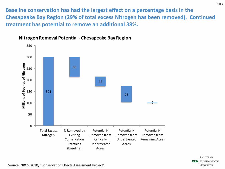
Baseline conservation has had the largest effect on a percentage basis in the Chesapeake Bay Region (29% of total excess Nitrogen has been removed). Continued treatment has potential to remove an additional 38%.
103
Source: NRCS, 2010, “Conservation Effects Assessment Project”.
301
86
42
69
2
0
50
100
150
200
250
300
350
Total Excess Nitrogen
N Removed by Existing
Conservation
Practices (baseline)
Potential N Removed from
Critically
Undertreated Acres
Potential N Removed from Undertreated
Acres
Potential N Removed from
Remaining Acres
Mill
ion
s o
f P
ou
nd
s o
f N
itro
gen
Nitrogen Removal Potential - Chesapeake Bay Region
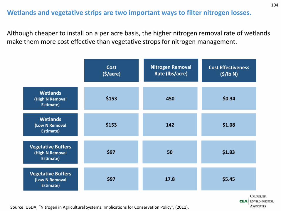
Wetlands and vegetative strips are two important ways to filter nitrogen losses.
Wetlands (High N Removal
Estimate)
Vegetative Buffers (High N Removal
Estimate)
Cost ($/acre)
Nitrogen Removal Rate (lbs/acre)
Cost Effectiveness ($/lb N)
Wetlands (Low N Removal
Estimate)
$153 450 $0.34
$153 142 $1.08
$97 50 $1.83
Vegetative Buffers (Low N Removal
Estimate)
$97 17.8 $5.45
Source: USDA, “Nitrogen in Agricultural Systems: Implications for Conservation Policy”, (2011).
104
Although cheaper to install on a per acre basis, the higher nitrogen removal rate of wetlands make them more cost effective than vegetative strops for nitrogen management.
Nitrogen mitigation Executive summary > GHG emissions > GHG mitigation > Nitrogen pollution > Nitrogen mitigation
105
- Logic model - Diet and behavior - Best management
practices - Lessons from Europe
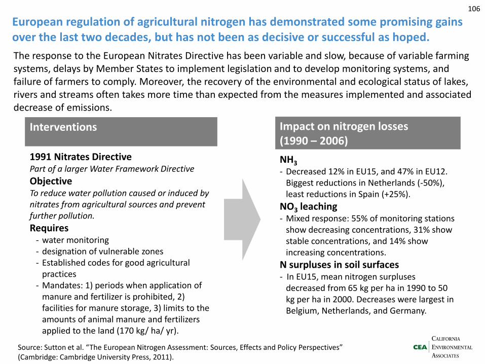
European regulation of agricultural nitrogen has demonstrated some promising gains over the last two decades, but has not been as decisive or successful as hoped.
106
Interventions
1991 Nitrates Directive Part of a larger Water Framework Directive
Objective To reduce water pollution caused or induced by nitrates from agricultural sources and prevent further pollution.
Requires - water monitoring - designation of vulnerable zones - Established codes for good agricultural
practices - Mandates: 1) periods when application of
manure and fertilizer is prohibited, 2) facilities for manure storage, 3) limits to the amounts of animal manure and fertilizers applied to the land (170 kg/ ha/ yr).
Impact on nitrogen losses (1990 – 2006)
NH3
- Decreased 12% in EU15, and 47% in EU12. Biggest reductions in Netherlands (-50%), least reductions in Spain (+25%).
NO3 leaching - Mixed response: 55% of monitoring stations
show decreasing concentrations, 31% show stable concentrations, and 14% show increasing concentrations.
N surpluses in soil surfaces - In EU15, mean nitrogen surpluses
decreased from 65 kg per ha in 1990 to 50 kg per ha in 2000. Decreases were largest in Belgium, Netherlands, and Germany.
The response to the European Nitrates Directive has been variable and slow, because of variable farming systems, delays by Member States to implement legislation and to develop monitoring systems, and failure of farmers to comply. Moreover, the recovery of the environmental and ecological status of lakes, rivers and streams often takes more time than expected from the measures implemented and associated decrease of emissions.
Source: Sutton et al. “The European Nitrogen Assessment: Sources, Effects and Policy Perspectives” (Cambridge: Cambridge University Press, 2011).
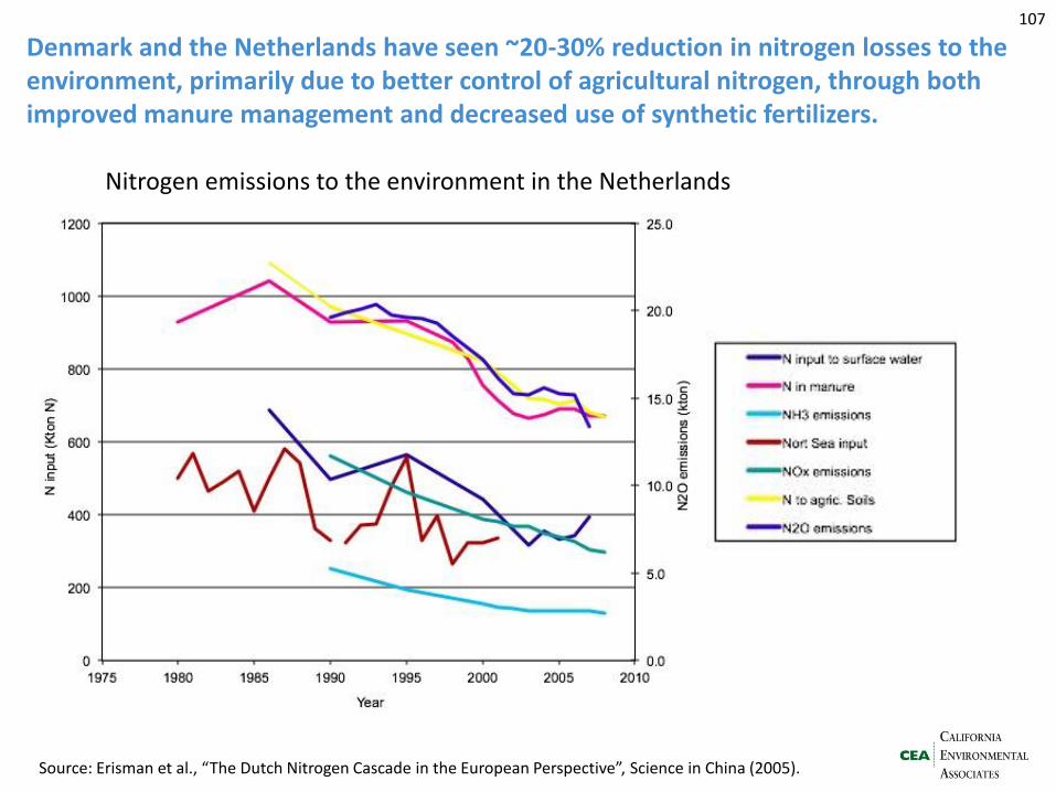
Denmark and the Netherlands have seen ~20-30% reduction in nitrogen losses to the environment, primarily due to better control of agricultural nitrogen, through both improved manure management and decreased use of synthetic fertilizers.
107
Source: Erisman et al., “The Dutch Nitrogen Cascade in the European Perspective”, Science in China (2005).
Nitrogen emissions to the environment in the Netherlands
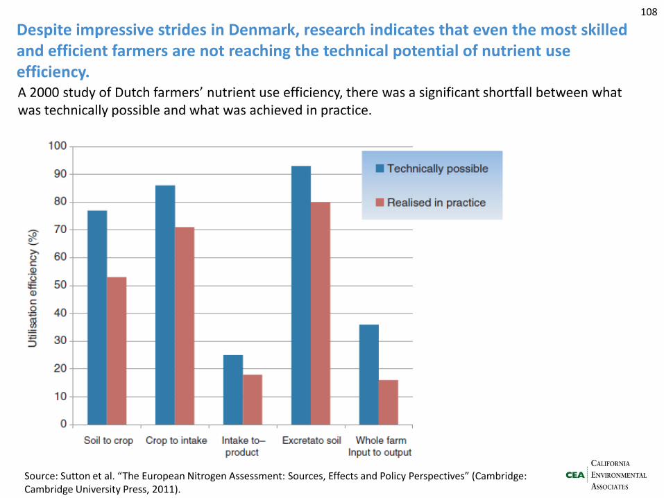
Despite impressive strides in Denmark, research indicates that even the most skilled and efficient farmers are not reaching the technical potential of nutrient use efficiency.
108
Source: Sutton et al. “The European Nitrogen Assessment: Sources, Effects and Policy Perspectives” (Cambridge: Cambridge University Press, 2011).
A 2000 study of Dutch farmers’ nutrient use efficiency, there was a significant shortfall between what was technically possible and what was achieved in practice.
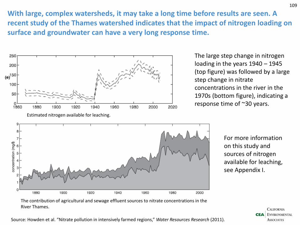
With large, complex watersheds, it may take a long time before results are seen. A recent study of the Thames watershed indicates that the impact of nitrogen loading on surface and groundwater can have a very long response time.
The large step change in nitrogen loading in the years 1940 – 1945 (top figure) was followed by a large step change in nitrate concentrations in the river in the 1970s (bottom figure), indicating a response time of ~30 years.
109
The contribution of agricultural and sewage effluent sources to nitrate concentrations in the River Thames.
Estimated nitrogen available for leaching.
Source: Howden et al. “Nitrate pollution in intensively farmed regions,” Water Resources Research (2011).
For more information on this study and sources of nitrogen available for leaching, see Appendix I.
Appendices
110

Appendix A:
Interviewees
111

Interviewees
Interviews completed
• Justin Baker, RTI International • Eric Davidson, Woods Hole Research Center • Otto Doering, Purdue University • Stephen DelGrosso, USDA – ARS • Jan Willem Erisman – Louis Bolk Institute (the Netherlands) • Marlen Eve, USDA Global Change Program • Erin Fitzgerald, Dairy Management Inc. • Dermot Hayes, Iowa State University • Jim Galloway, University of Virginia • Dan Liptzin, UC Davis • Sara Lewis, Sustainability Consortium • Brian Murray, Nicholas Institute • Lydia Olander and Alison Eagle, Nicholas Institute • Stephen Preston, USGS • Shaun Ragnauth, EPA • Debbie Reed, C-AGG • Karen Thomas and Sonja Brodt, UC Davis • Penelope Whitney, Resource Media • Tom Wirth, EPA
112
Appendix B:
Animal Populations
113
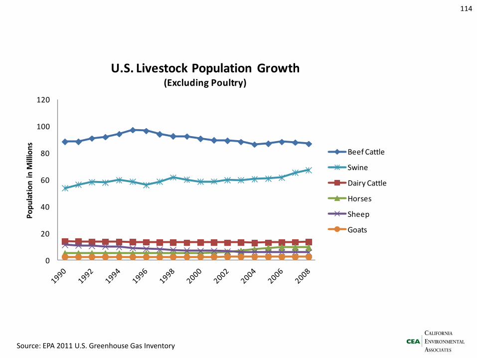
Source: EPA 2011 U.S. Greenhouse Gas Inventory
114
0
20
40
60
80
100
120
Po
pu
lati
on
in
Mill
ion
s
U.S. Livestock Population Growth (Excluding Poultry)
Beef Cattle
Swine
Dairy Cattle
Horses
Sheep
Goats
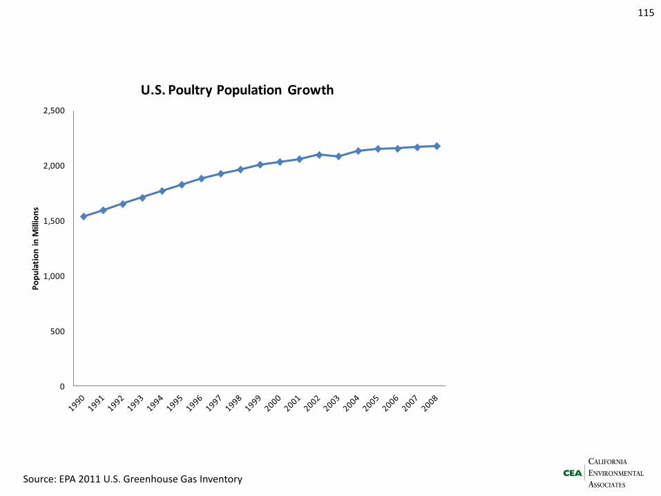
Source: EPA 2011 U.S. Greenhouse Gas Inventory
115
0
500
1,000
1,500
2,000
2,500
Po
pu
lati
on
in
Mill
ion
s
U.S. Poultry Population Growth
Appendix C:
Scenarios detail
116
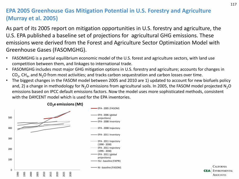
EPA 2005 Greenhouse Gas Mitigation Potential in U.S. Forestry and Agriculture (Murray et al. 2005)
As part of its 2005 report on mitigation opportunities in U.S. forestry and agriculture, the U.S. EPA published a baseline set of projections for agricultural GHG emissions. These emissions were derived from the Forest and Agriculture Sector Optimization Model with Greenhouse Gases (FASOMGHG).
• FASOMGHG is a partial equilibrium economic model of the U.S. forest and agriculture sectors, with land use competition between them, and linkages to international trade.
• FASOMGHG includes most major GHG mitigation options in U.S. forestry and agriculture; accounts for changes in CO2, CH4, and N2O from most activities; and tracks carbon sequestration and carbon losses over time.
• The biggest changes in the FASOM model between 2005 and 2010 are 1) updated to account for new biofuels policy and, 2) a change in methodology for N2O emissions from agricultural soils. In 2005, the FASOM model projected N2O emissions based on IPCC default emissions factors. Now the model uses more sophisticated methods, consistent with the DAYCENT model which is used for the EPA inventories.
117
0
100
200
300
400
500
1990
1995
2000
2005
2010
2015
2020
2025
2030
CO2e emissions (Mt)EPA - 2005 (FASOM)
EPA - 2006 (global projections)
EPA - 2008 Inventory
EPA - 2008 trajectory
EPA - 2011 Inventory
EPA - 2011 trajectory (1990 - 2030)
EPA - 2011 trajectory (1995 - 2030)
EPA - 2011 (global projections)
ISU - baseline (FAPRI)
NI - baseline (FASOM)
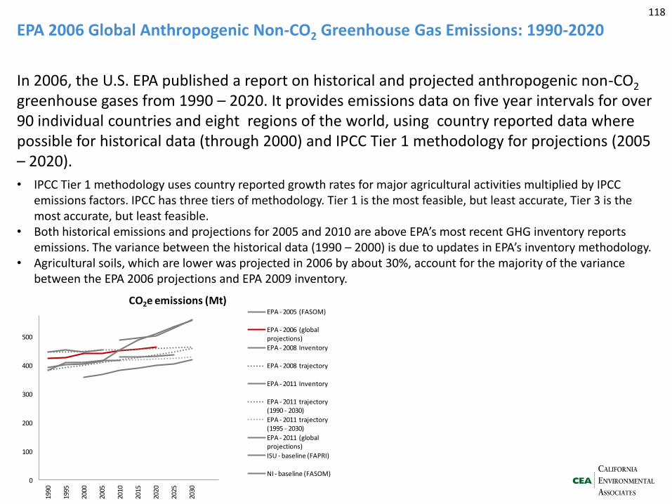
EPA 2006 Global Anthropogenic Non-CO2 Greenhouse Gas Emissions: 1990-2020
In 2006, the U.S. EPA published a report on historical and projected anthropogenic non-CO2 greenhouse gases from 1990 – 2020. It provides emissions data on five year intervals for over 90 individual countries and eight regions of the world, using country reported data where possible for historical data (through 2000) and IPCC Tier 1 methodology for projections (2005 – 2020).
• IPCC Tier 1 methodology uses country reported growth rates for major agricultural activities multiplied by IPCC emissions factors. IPCC has three tiers of methodology. Tier 1 is the most feasible, but least accurate, Tier 3 is the most accurate, but least feasible.
• Both historical emissions and projections for 2005 and 2010 are above EPA’s most recent GHG inventory reports emissions. The variance between the historical data (1990 – 2000) is due to updates in EPA’s inventory methodology.
• Agricultural soils, which are lower was projected in 2006 by about 30%, account for the majority of the variance between the EPA 2006 projections and EPA 2009 inventory.
118
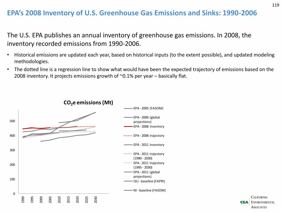
EPA’s 2008 Inventory of U.S. Greenhouse Gas Emissions and Sinks: 1990-2006
The U.S. EPA publishes an annual inventory of greenhouse gas emissions. In 2008, the inventory recorded emissions from 1990-2006.
• Historical emissions are updated each year, based on historical inputs (to the extent possible), and updated modeling methodologies.
• The dotted line is a regression line to show what would have been the expected trajectory of emissions based on the 2008 inventory. It projects emissions growth of ~0.1% per year – basically flat.
119
0
100
200
300
400
500
1990
1995
2000
2005
2010
2015
2020
2025
2030
CO2e emissions (Mt)EPA - 2005 (FASOM)
EPA - 2006 (global projections)
EPA - 2008 Inventory
EPA - 2008 trajectory
EPA - 2011 Inventory
EPA - 2011 trajectory (1990 - 2030)
EPA - 2011 trajectory (1995 - 2030)
EPA - 2011 (global projections)
ISU - baseline (FAPRI)
NI - baseline (FASOM)
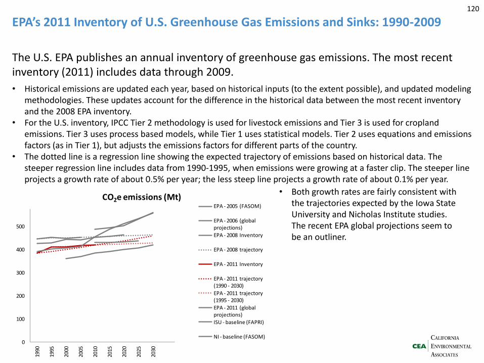
EPA’s 2011 Inventory of U.S. Greenhouse Gas Emissions and Sinks: 1990-2009
The U.S. EPA publishes an annual inventory of greenhouse gas emissions. The most recent inventory (2011) includes data through 2009.
• Historical emissions are updated each year, based on historical inputs (to the extent possible), and updated modeling methodologies. These updates account for the difference in the historical data between the most recent inventory and the 2008 EPA inventory.
• For the U.S. inventory, IPCC Tier 2 methodology is used for livestock emissions and Tier 3 is used for cropland emissions. Tier 3 uses process based models, while Tier 1 uses statistical models. Tier 2 uses equations and emissions factors (as in Tier 1), but adjusts the emissions factors for different parts of the country.
• The dotted line is a regression line showing the expected trajectory of emissions based on historical data. The steeper regression line includes data from 1990-1995, when emissions were growing at a faster clip. The steeper line projects a growth rate of about 0.5% per year; the less steep line projects a growth rate of about 0.1% per year.
120
• Both growth rates are fairly consistent with the trajectories expected by the Iowa State University and Nicholas Institute studies. The recent EPA global projections seem to be an outliner.
0
100
200
300
400
500
1990
1995
2000
2005
2010
2015
2020
2025
2030
CO2e emissions (Mt)EPA - 2005 (FASOM)
EPA - 2006 (global projections)
EPA - 2008 Inventory
EPA - 2008 trajectory
EPA - 2011 Inventory
EPA - 2011 trajectory (1990 - 2030)
EPA - 2011 trajectory (1995 - 2030)
EPA - 2011 (global projections)
ISU - baseline (FAPRI)
NI - baseline (FASOM)
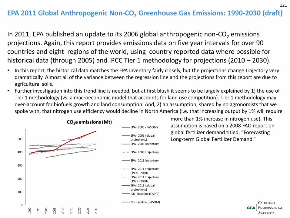
EPA 2011 Global Anthropogenic Non-CO2 Greenhouse Gas Emissions: 1990-2030 (draft)
In 2011, EPA published an update to its 2006 global anthropogenic non-CO2 emissions projections. Again, this report provides emissions data on five year intervals for over 90 countries and eight regions of the world, using country reported data where possible for historical data (through 2005) and IPCC Tier 1 methodology for projections (2010 – 2030).
• In this report, the historical data matches the EPA inventory fairly closely, but the projections change trajectory very dramatically. Almost all of the variance between the regression line and the projections from this report are due to agricultural soils.
• Further investigation into this trend line is needed, but at first blush it seems to be largely explained by 1) the use of Tier 1 methodology (vs. a macroeconomic model that accounts for land use competition). Tier 1 methodology may over-account for biofuels growth and land consumption. And, 2) an assumption, shared by no agronomists that we spoke with, that nitrogen use efficiency would decline in North America (i.e. that increasing output by 1% will require
121
0
100
200
300
400
500
1990
1995
2000
2005
2010
2015
2020
2025
2030
CO2e emissions (Mt)EPA - 2005 (FASOM)
EPA - 2006 (global projections)
EPA - 2008 Inventory
EPA - 2008 trajectory
EPA - 2011 Inventory
EPA - 2011 trajectory (1990 - 2030)
EPA - 2011 trajectory (1995 - 2030)
EPA - 2011 (global projections)
ISU - baseline (FAPRI)
NI - baseline (FASOM)
more than 1% increase in nitrogen use). This assumption is based on a 2008 FAO report on global fertilizer demand titled, “Forecasting Long-term Global Fertilizer Demand.”
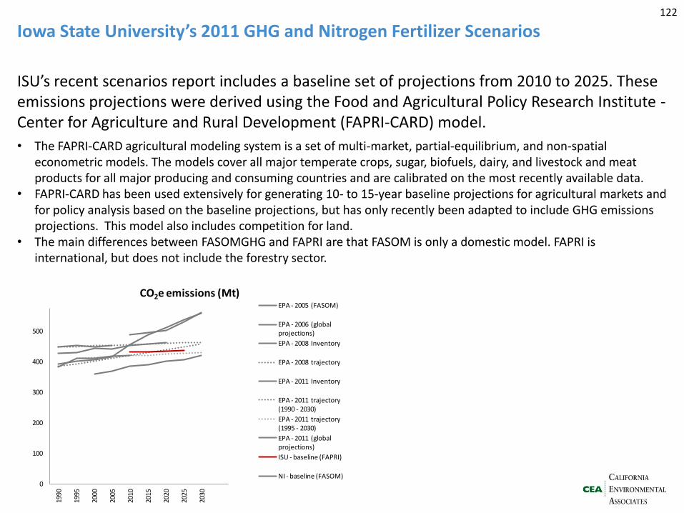
Iowa State University’s 2011 GHG and Nitrogen Fertilizer Scenarios
ISU’s recent scenarios report includes a baseline set of projections from 2010 to 2025. These emissions projections were derived using the Food and Agricultural Policy Research Institute - Center for Agriculture and Rural Development (FAPRI-CARD) model.
• The FAPRI-CARD agricultural modeling system is a set of multi-market, partial-equilibrium, and non-spatial econometric models. The models cover all major temperate crops, sugar, biofuels, dairy, and livestock and meat products for all major producing and consuming countries and are calibrated on the most recently available data.
• FAPRI-CARD has been used extensively for generating 10- to 15-year baseline projections for agricultural markets and for policy analysis based on the baseline projections, but has only recently been adapted to include GHG emissions projections. This model also includes competition for land.
• The main differences between FASOMGHG and FAPRI are that FASOM is only a domestic model. FAPRI is international, but does not include the forestry sector.
122
0
100
200
300
400
500
1990
1995
2000
2005
2010
2015
2020
2025
2030
CO2e emissions (Mt)EPA - 2005 (FASOM)
EPA - 2006 (global projections)
EPA - 2008 Inventory
EPA - 2008 trajectory
EPA - 2011 Inventory
EPA - 2011 trajectory (1990 - 2030)
EPA - 2011 trajectory (1995 - 2030)
EPA - 2011 (global projections)
ISU - baseline (FAPRI)
NI - baseline (FASOM)
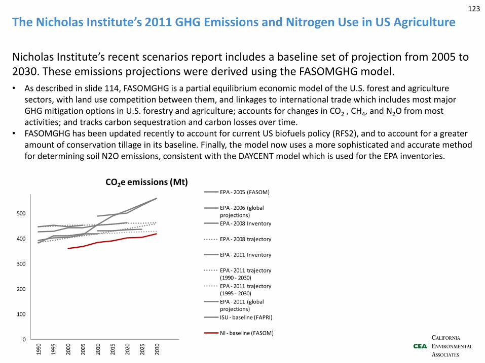
The Nicholas Institute’s 2011 GHG Emissions and Nitrogen Use in US Agriculture
Nicholas Institute’s recent scenarios report includes a baseline set of projection from 2005 to 2030. These emissions projections were derived using the FASOMGHG model.
• As described in slide 114, FASOMGHG is a partial equilibrium economic model of the U.S. forest and agriculture sectors, with land use competition between them, and linkages to international trade which includes most major GHG mitigation options in U.S. forestry and agriculture; accounts for changes in CO2 , CH4, and N2O from most activities; and tracks carbon sequestration and carbon losses over time.
• FASOMGHG has been updated recently to account for current US biofuels policy (RFS2), and to account for a greater amount of conservation tillage in its baseline. Finally, the model now uses a more sophisticated and accurate method for determining soil N2O emissions, consistent with the DAYCENT model which is used for the EPA inventories.
123
0
100
200
300
400
500
1990
1995
2000
2005
2010
2015
2020
2025
2030
CO2e emissions (Mt)EPA - 2005 (FASOM)
EPA - 2006 (global projections)
EPA - 2008 Inventory
EPA - 2008 trajectory
EPA - 2011 Inventory
EPA - 2011 trajectory (1990 - 2030)
EPA - 2011 trajectory (1995 - 2030)
EPA - 2011 (global projections)
ISU - baseline (FAPRI)
NI - baseline (FASOM)
Appendix D:
Global and U.S. greenhouse gas trends
124
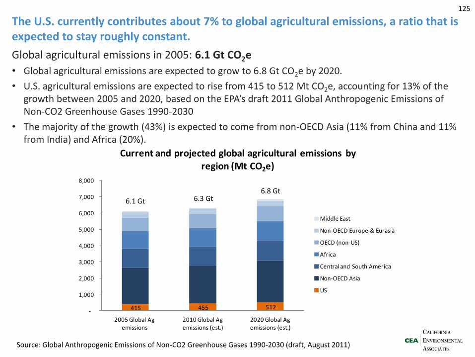
The U.S. currently contributes about 7% to global agricultural emissions, a ratio that is expected to stay roughly constant.
Global agricultural emissions in 2005: 6.1 Gt CO2e
• Global agricultural emissions are expected to grow to 6.8 Gt CO2e by 2020.
• U.S. agricultural emissions are expected to rise from 415 to 512 Mt CO2e, accounting for 13% of the growth between 2005 and 2020, based on the EPA’s draft 2011 Global Anthropogenic Emissions of Non-CO2 Greenhouse Gases 1990-2030
• The majority of the growth (43%) is expected to come from non-OECD Asia (11% from China and 11% from India) and Africa (20%).
Source: Global Anthropogenic Emissions of Non-CO2 Greenhouse Gases 1990-2030 (draft, August 2011)
125
415 455 512 -
1,000
2,000
3,000
4,000
5,000
6,000
7,000
8,000
2005 Global Ag emissions
2010 Global Ag emissions (est.)
2020 Global Ag emissions (est.)
Current and projected global agricultural emissions by region (Mt CO2e)
Middle East
Non-OECD Europe & Eurasia
OECD (non-US)
Africa
Central and South America
Non-OECD Asia
US
6.1 Gt 6.3 Gt 6.8 Gt
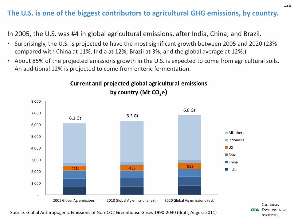
The U.S. is one of the biggest contributors to agricultural GHG emissions, by country.
In 2005, the U.S. was #4 in global agricultural emissions, after India, China, and Brazil.
• Surprisingly, the U.S. is projected to have the most significant growth between 2005 and 2020 (23% compared with China at 11%, India at 12%, Brazil at 3%, and the global average at 12%.)
• About 85% of the projected emissions growth in the U.S. is expected to come from agricultural soils. An additional 12% is projected to come from enteric fermentation.
Source: Global Anthropogenic Emissions of Non-CO2 Greenhouse Gases 1990-2030 (draft, August 2011)
126
415 455 512
-
1,000
2,000
3,000
4,000
5,000
6,000
7,000
8,000
2005 Global Ag emissions 2010 Global Ag emissions (est.) 2020 Global Ag emissions (est.)
Current and projected global agricultural emissions
by country (Mt CO2e)
All others
Indonesia
US
Brazil
China
India
6.1 Gt 6.3 Gt 6.8 Gt
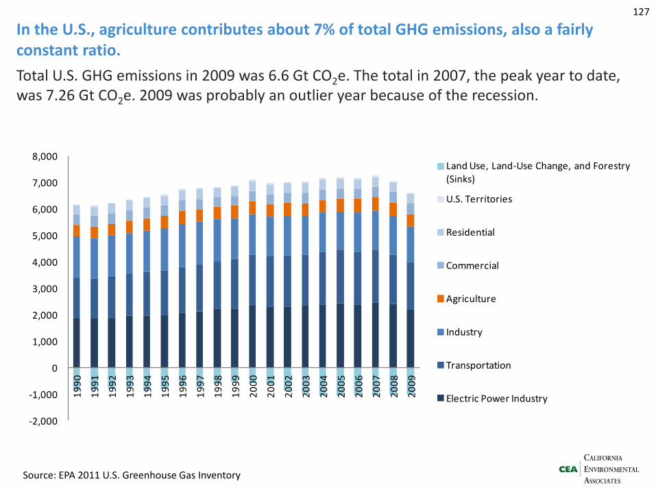
In the U.S., agriculture contributes about 7% of total GHG emissions, also a fairly constant ratio.
Total U.S. GHG emissions in 2009 was 6.6 Gt CO2e. The total in 2007, the peak year to date, was 7.26 Gt CO2e. 2009 was probably an outlier year because of the recession.
-2,000
-1,000
0
1,000
2,000
3,000
4,000
5,000
6,000
7,000
8,000
19
90
19
91
19
92
19
93
19
94
19
95
19
96
19
97
19
98
19
99
20
00
20
01
20
02
20
03
20
04
20
05
20
06
20
07
20
08
20
09
Land Use, Land-Use Change, and Forestry (Sinks)
U.S. Territories
Residential
Commercial
Agriculture
Industry
Transportation
Electric Power Industry
Source: EPA 2011 U.S. Greenhouse Gas Inventory
127

Appendix E:
Uncertainty
128

Livestock Greenhouse Gas Emission Estimates and Uncertainty Intervals, 2008
Source Estimate Lower Bound Upper Bound Range Lower Bound Upper Bound
Tg CO2e
CH4 enteric fermentation 141 125 166 41 -11 +18
CH4 managed waste and grazed land 48 39 57 18 -18 +20
N2O managed waste 14 12 18 6 -16 +24
N2O grazed land 62 39 156 117 -37 +153
CO2 grazed land remaining grazed land -5 -7 -3 4 -53 +42
CO2 land converted to grazed land -27 -29 -24 5 -8 +9
Net Emissions 234 204 332 128 -13 +42
Tg CO 2e percent
Agriculture and Forestry Greenhouse Gas Emissions Estimates and Uncertainty Intervals, 2008
Source Estimate Lower Bound Upper Bound Range Lower Bound Upper Bound
Tg CO2e
Livestock 203 185 230 45 -9 +14
Crops1 154 84 215 131 -34 +71
Grassland1 33 5 132 127 -84 +298
Net Emissions 390 274 577 303 -30 +48
Tg CO 2e percent
Both cropland and grassland (grazed land) emissions have high levels of uncertainty. Grassland emissions are the least certain, but emissions are greater for cropland; thus cropland and grassland contributes about equally to overall uncertainty.
Note: Negative numbers indicate net sequestration. 1 - Includes sequestration in agricultural soils. Livestock and Grassland (grazed land) emissions are combined in the second table.
Source: USDA Agriculture and Forestry Greenhouse Gas Inventory: 1990-2008
129
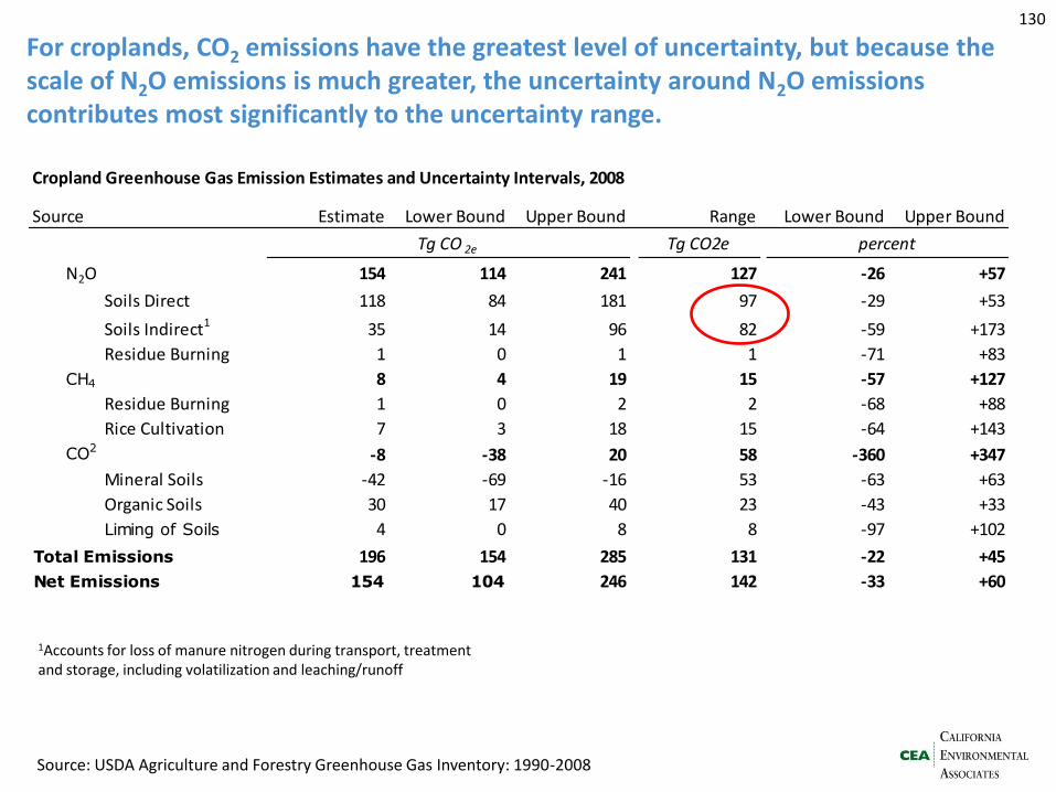
Cropland Greenhouse Gas Emission Estimates and Uncertainty Intervals, 2008
Source Estimate Lower Bound Upper Bound Range Lower Bound Upper Bound
Tg CO2e
N2O 154 114 241 127 -26 +57
Soils Direct 118 84 181 97 -29 +53
Soils Indirect1 35 14 96 82 -59 +173
Residue Burning 1 0 1 1 -71 +83
CH4 8 4 19 15 -57 +127
Residue Burning 1 0 2 2 -68 +88
Rice Cultivation 7 3 18 15 -64 +143
CO2 -8 -38 20 58 -360 +347
Mineral Soils -42 -69 -16 53 -63 +63
Organic Soils 30 17 40 23 -43 +33
Liming of Soils 4 0 8 8 -97 +102
Total Emissions 196 154 285 131 -22 +45
Net Emissions 154 104 246 142 -33 +60
Tg CO 2e percent
For croplands, CO2 emissions have the greatest level of uncertainty, but because the scale of N2O emissions is much greater, the uncertainty around N2O emissions contributes most significantly to the uncertainty range.
Source: USDA Agriculture and Forestry Greenhouse Gas Inventory: 1990-2008
1Accounts for loss of manure nitrogen during transport, treatment and storage, including volatilization and leaching/runoff
130
Appendix F:
Cropland and Livestock emissions back-up
131
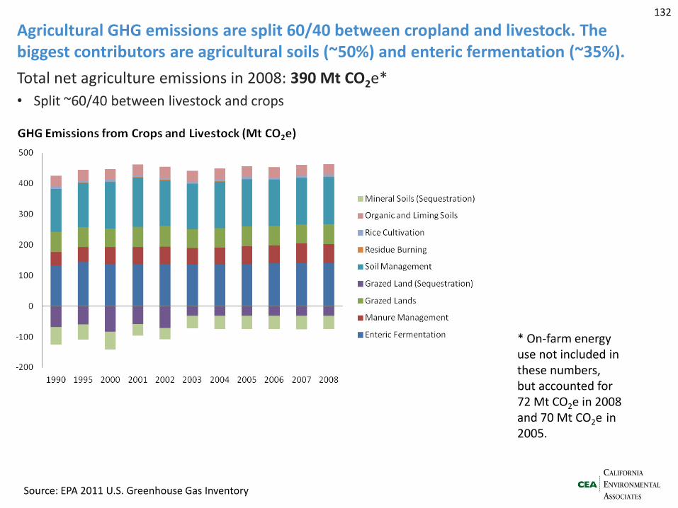
Agricultural GHG emissions are split 60/40 between cropland and livestock. The biggest contributors are agricultural soils (~50%) and enteric fermentation (~35%).
Total net agriculture emissions in 2008: 390 Mt CO2e*
• Split ~60/40 between livestock and crops
Source: EPA 2011 U.S. Greenhouse Gas Inventory
* On-farm energy use not included in these numbers, but accounted for 72 Mt CO2e in 2008 and 70 Mt CO2e in 2005.
132
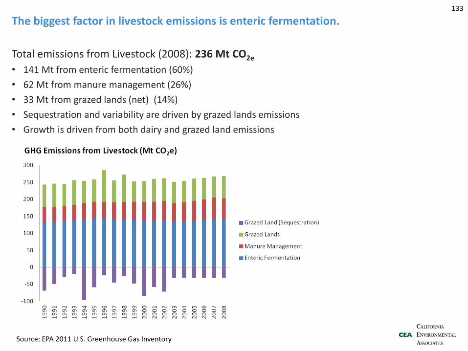
The biggest factor in livestock emissions is enteric fermentation.
Total emissions from Livestock (2008): 236 Mt CO2e
• 141 Mt from enteric fermentation (60%)
• 62 Mt from manure management (26%)
• 33 Mt from grazed lands (net) (14%)
• Sequestration and variability are driven by grazed lands emissions
• Growth is driven from both dairy and grazed land emissions
Source: EPA 2011 U.S. Greenhouse Gas Inventory
133
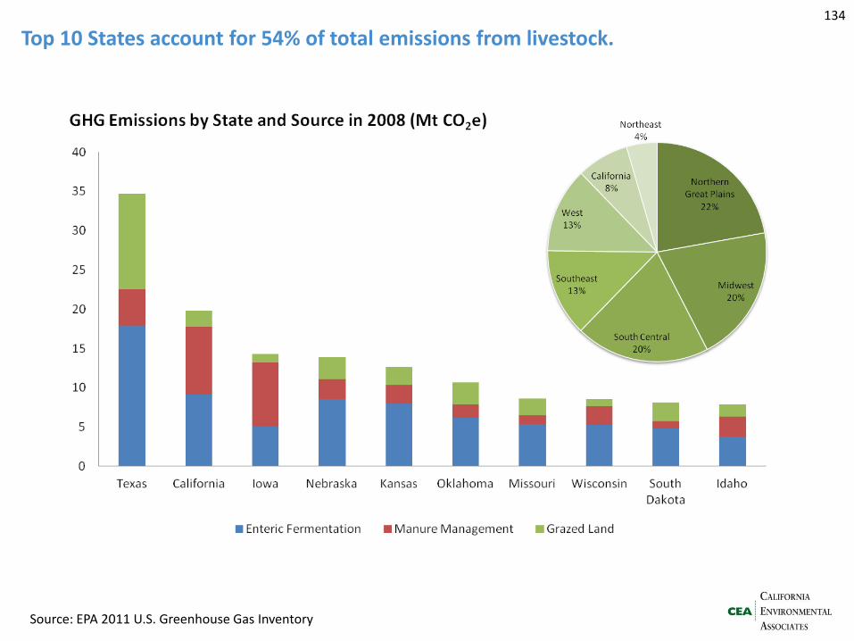
Top 10 States account for 54% of total emissions from livestock.
Source: EPA 2011 U.S. Greenhouse Gas Inventory
134
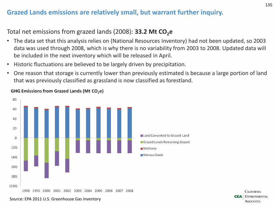
Grazed Lands emissions are relatively small, but warrant further inquiry.
Total net emissions from grazed lands (2008): 33.2 Mt CO2e
• The data set that this analysis relies on (National Resources Inventory) had not been updated, so 2003 data was used through 2008, which is why there is no variability from 2003 to 2008. Updated data will be included in the next inventory which will be released in April.
• Historic fluctuations are believed to be largely driven by precipitation.
• One reason that storage is currently lower than previously estimated is because a large portion of land that was previously classified as grassland is now classified as forestland.
Source: EPA 2011 U.S. Greenhouse Gas Inventory
135
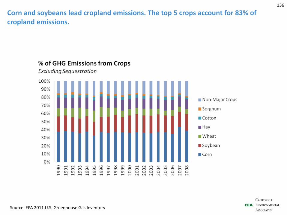
Corn and soybeans lead cropland emissions. The top 5 crops account for 83% of cropland emissions.
Source: EPA 2011 U.S. Greenhouse Gas Inventory
136
Appendix G:
Nitrogen sources back-up
137
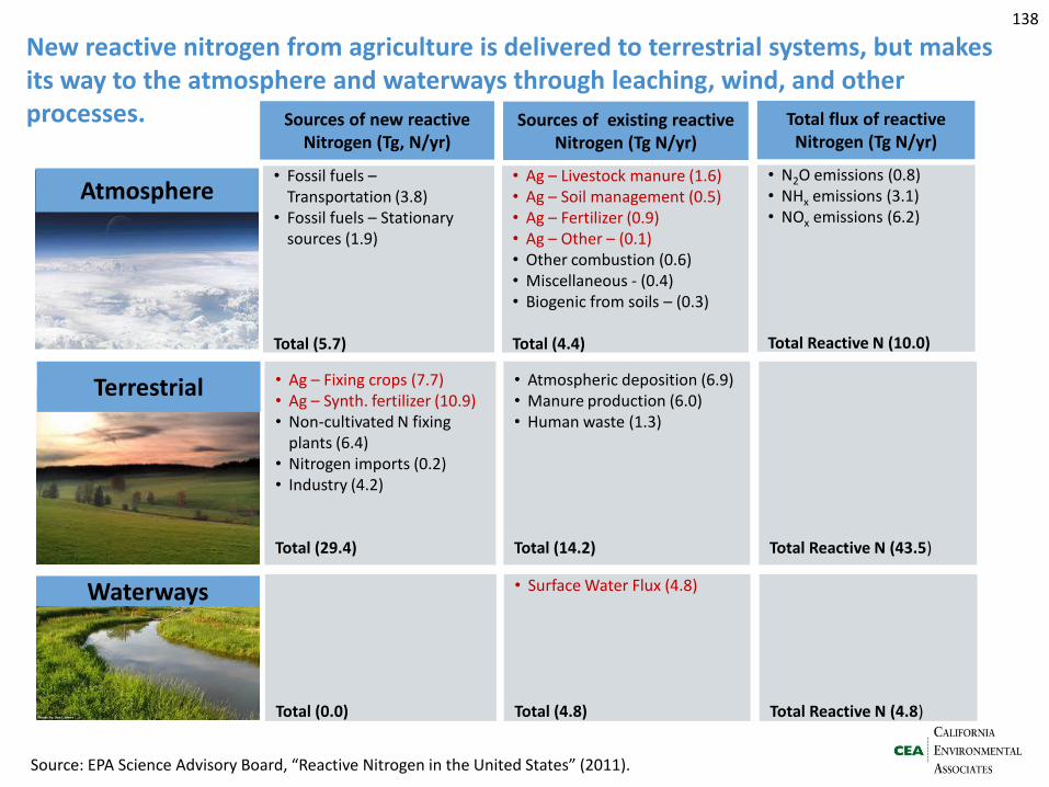
New reactive nitrogen from agriculture is delivered to terrestrial systems, but makes its way to the atmosphere and waterways through leaching, wind, and other processes.
Atmosphere
Terrestrial
Waterways
Sources of new reactive Nitrogen (Tg, N/yr)
Sources of existing reactive Nitrogen (Tg N/yr)
Total flux of reactive Nitrogen (Tg N/yr)
• Ag – Livestock manure (1.6) • Ag – Soil management (0.5) • Ag – Fertilizer (0.9) • Ag – Other – (0.1) • Other combustion (0.6) • Miscellaneous - (0.4) • Biogenic from soils – (0.3) Total (4.4)
• Fossil fuels – Transportation (3.8)
• Fossil fuels – Stationary sources (1.9)
Total (5.7)
• N2O emissions (0.8) • NHx emissions (3.1) • NOx emissions (6.2) Total Reactive N (10.0)
• Atmospheric deposition (6.9) • Manure production (6.0) • Human waste (1.3) Total (14.2)
• Ag – Fixing crops (7.7) • Ag – Synth. fertilizer (10.9) • Non-cultivated N fixing
plants (6.4) • Nitrogen imports (0.2) • Industry (4.2) Total (29.4)
Total Reactive N (43.5)
• Surface Water Flux (4.8) Total (4.8)
Total (0.0)
Total Reactive N (4.8)
Source: EPA Science Advisory Board, “Reactive Nitrogen in the United States” (2011).
138
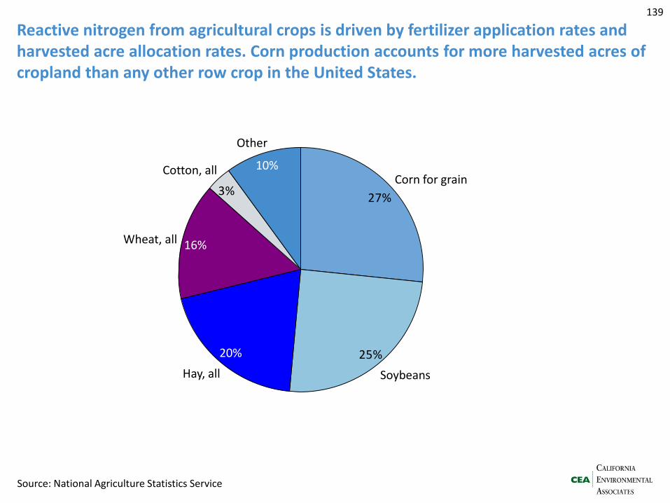
Reactive nitrogen from agricultural crops is driven by fertilizer application rates and harvested acre allocation rates. Corn production accounts for more harvested acres of cropland than any other row crop in the United States.
3%
25%
27%
Wheat, all
10%
20%
Corn for grain Cotton, all
Hay, all Soybeans
16%
Other
139
Source: National Agriculture Statistics Service
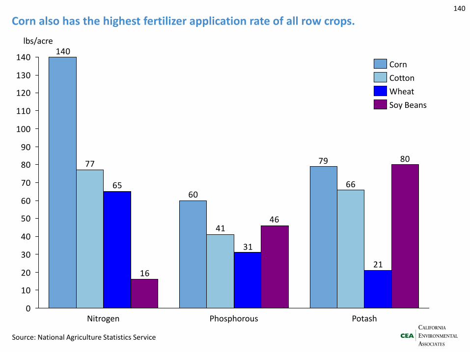
Corn also has the highest fertilizer application rate of all row crops.
79
60
140
66
41
77
21
31
65
80
46
16
0
10
20
30
40
50
60
70
80
90
100
110
120
130
140
Potash Phosphorous Nitrogen
lbs/acre
Soy Beans
Wheat
Cotton
Corn
Source: National Agriculture Statistics Service
140
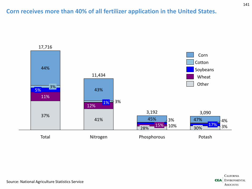
Corn receives more than 40% of all fertilizer application in the United States.
44%
3%
Total
17,716
37%
11%
5%
4% 47%
Phosphorous
3,192
28% 15% 10%
3% 45%
Nitrogen
3%
41%
43%
12%
11,434
1%
3% 17% 30%
Potash
3,090
Soybeans
Corn
Cotton
Other
Wheat
141
Source: National Agriculture Statistics Service
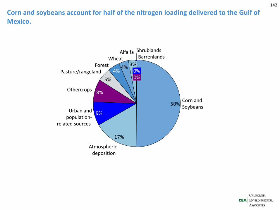
Corn and soybeans account for half of the nitrogen loading delivered to the Gulf of Mexico.
4%
5%
17%
50%
0%
Alfalfa
3% Wheat
Forest 4% Pasture/rangeland
Othercrops 8%
Urban and population-
related sources
9%
Atmospheric deposition
Corn and Soybeans
Barrenlands
0%
Shrublands
142
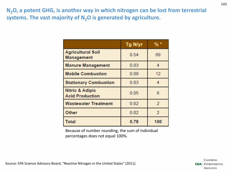
N2O, a potent GHG, is another way in which nitrogen can be lost from terrestrial systems. The vast majority of N2O is generated by agriculture.
143
Source: EPA Science Advisory Board, “Reactive Nitrogen in the United States” (2011).
Because of number rounding, the sum of individual percentages does not equal 100%.
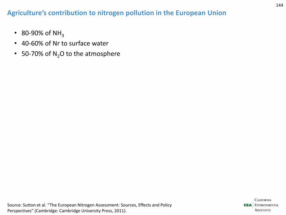
Agriculture’s contribution to nitrogen pollution in the European Union
• 80-90% of NH3
• 40-60% of Nr to surface water
• 50-70% of N2O to the atmosphere
144
Source: Sutton et al. “The European Nitrogen Assessment: Sources, Effects and Policy Perspectives” (Cambridge: Cambridge University Press, 2011).
Appendix H:
Nitrogen mitigation back-up
145
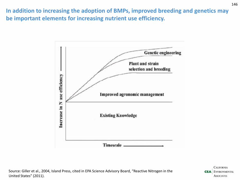
In addition to increasing the adoption of BMPs, improved breeding and genetics may be important elements for increasing nutrient use efficiency.
146
Source: Giller et al., 2004, Island Press, cited in EPA Science Advisory Board, “Reactive Nitrogen in the United States” (2011).
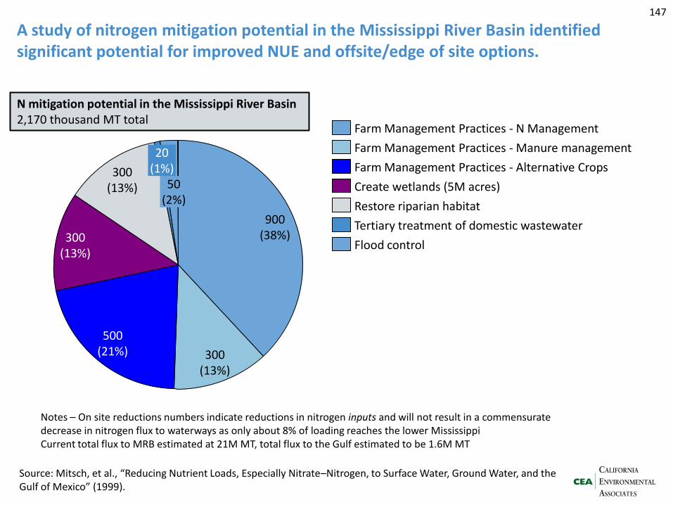
A study of nitrogen mitigation potential in the Mississippi River Basin identified significant potential for improved NUE and offsite/edge of site options.
300 (13%)
900 (38%)
300 (13%)
20 (1%)
300 (13%)
500 (21%)
50 (2%)
Farm Management Practices - N Management
Farm Management Practices - Manure management
Create wetlands (5M acres)
Farm Management Practices - Alternative Crops
Restore riparian habitat
Tertiary treatment of domestic wastewater
Flood control
N mitigation potential in the Mississippi River Basin 2,170 thousand MT total
Source: Mitsch, et al., “Reducing Nutrient Loads, Especially Nitrate–Nitrogen, to Surface Water, Ground Water, and the Gulf of Mexico” (1999).
Notes – On site reductions numbers indicate reductions in nitrogen inputs and will not result in a commensurate decrease in nitrogen flux to waterways as only about 8% of loading reaches the lower Mississippi Current total flux to MRB estimated at 21M MT, total flux to the Gulf estimated to be 1.6M MT
147
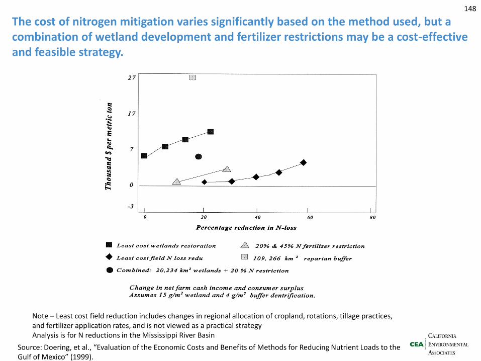
The cost of nitrogen mitigation varies significantly based on the method used, but a combination of wetland development and fertilizer restrictions may be a cost-effective and feasible strategy.
Source: Doering, et al., “Evaluation of the Economic Costs and Benefits of Methods for Reducing Nutrient Loads to the Gulf of Mexico” (1999).
Note – Least cost field reduction includes changes in regional allocation of cropland, rotations, tillage practices, and fertilizer application rates, and is not viewed as a practical strategy Analysis is for N reductions in the Mississippi River Basin
148
Appendix I:
Further detail on nitrogen in the River Thames
149
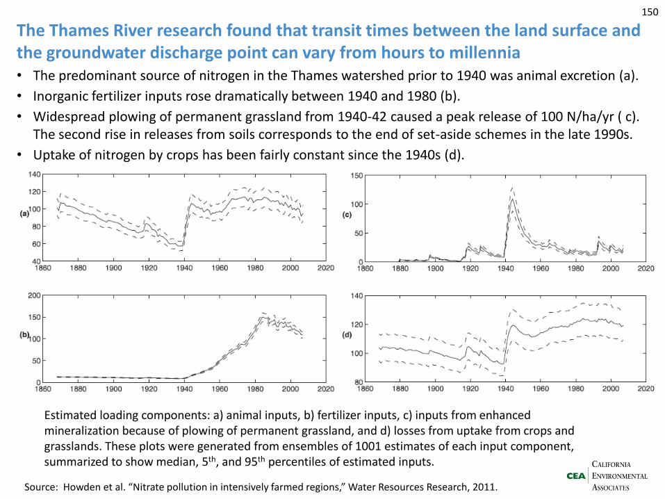
The Thames River research found that transit times between the land surface and the groundwater discharge point can vary from hours to millennia
150
Estimated loading components: a) animal inputs, b) fertilizer inputs, c) inputs from enhanced mineralization because of plowing of permanent grassland, and d) losses from uptake from crops and grasslands. These plots were generated from ensembles of 1001 estimates of each input component, summarized to show median, 5th, and 95th percentiles of estimated inputs.
Source: Howden et al. “Nitrate pollution in intensively farmed regions,” Water Resources Research, 2011.
• The predominant source of nitrogen in the Thames watershed prior to 1940 was animal excretion (a).
• Inorganic fertilizer inputs rose dramatically between 1940 and 1980 (b).
• Widespread plowing of permanent grassland from 1940-42 caused a peak release of 100 N/ha/yr ( c). The second rise in releases from soils corresponds to the end of set-aside schemes in the late 1990s.
• Uptake of nitrogen by crops has been fairly constant since the 1940s (d).
Top Related