


Languages
Pages
Legal


GRAVITY THEORIES AT LARGE NUMBER OF DIMENSIONS
A THESIS SUBMITTED TOTHE GRADUATE SCHOOL OF NATURAL AND APPLIED SCIENCES
OFMIDDLE EAST TECHNICAL UNIVERSITY
BY
GÖKÇEN DENIZ ÖZEN
IN PARTIAL FULFILLMENT OF THE REQUIREMENTSFOR
THE DEGREE OF DOCTOR OF PHILOSOPHYIN
PHYSICS
AUGUST 2021


Approval of the thesis:
GRAVITY THEORIES AT LARGE NUMBER OF DIMENSIONS
submitted by GÖKÇEN DENIZ ÖZEN in partial fulfillment of the requirementsfor the degree of Doctor of Philosophy in Physics Department, Middle EastTechnical University by,
Prof. Dr. Halil KalıpçılarDean, Graduate School of Natural and Applied Sciences
Prof. Dr. Seçkin KürkçüogluHead of Department, Physics
Prof. Dr. Bayram TekinSupervisor, Physics Department, METU
Examining Committee Members:
Prof. Dr. Atalay KarasuPhysics Department, METU
Prof. Dr. Bayram TekinPhysics Department, METU
Assoc. Prof. Dr. Ismet YurdusenMathematics Department, Hacettepe University
Prof. Dr. Ali Murat GülerPhysics Department, METU
Prof. Dr. Tahsin Çagrı SismanAstronautical Engineering, UTAA
Date: 13.08.2021

I hereby declare that all information in this document has been obtained andpresented in accordance with academic rules and ethical conduct. I also declarethat, as required by these rules and conduct, I have fully cited and referenced allmaterial and results that are not original to this work.
Name, Surname: Gökçen Denız Özen
Signature :
iv

ABSTRACT
GRAVITY THEORIES AT LARGE NUMBER OF DIMENSIONS
Özen, Gökçen Denız
Ph.D., Department of Physics
Supervisor: Prof. Dr. Bayram Tekin
August 2021, 103 pages
General Relativity is succesful in understanding the phenomena such as light bending
by the Sun and the perihelion precession of Mercury that could not be understood in
Newton’s gravity. Within solar system scales, General Relativity is a very powerful
theory but for very small or very large distances, the theory has non-renormalization
issues and lack of explanation of the accelerated expansion of the universe and the
galaxy rotation curves which give a hint at the need for modifications. In this thesis,
Born-Infeld type modifications of General Relativity are considered. In 1998 Deser
and Gibbons proposed Born-Infeld gravity theory that has some common features
with the Eddington’s gravitational action and the Born-Infeld electrodynamics. The
Born-Infeld gravity theory, like the other two, has a determinantal action but the free
variable of the theory is the metric not the connection as in the Eddington’s gravity
theory. In this thesis we have calculated the Wald entropy of the Born-Infeld gravity
theories and showed that this dynamical entropy reduces to the geometric Bekenstein-
Hawking entropy with the appropriate choice of effective gravitational constant. We
also discuss black hole entropy in generic dimensions for the Born-Infeld theories.
v
Keywords: Black holes, thermodynamics of black holes, nonlinear electrodynamics,
Born-Infeld gravity, Wald entropy, entropy in Born-Infeld gravity
vi

ÖZ
YÜKSEK SAYIDA BOYUTLARA SAHIP KÜTLE ÇEKIM TEORISI
Özen, Gökçen Denız
Doktora, Fizik Bölümü
Tez Yöneticisi: Prof. Dr. Bayram Tekin
Agustos 2021 , 103 sayfa
Genel Görelilik, Newton’un kütleçekiminde anlasılamayan Günes’in ısıgı bükmesi
ve Merkür’ün günberi devinimi gibi olguları anlamakta basarılıdır. Günes sistemi öl-
çeklerinde Genel Görelilik çok güçlü bir teoridir, ancak çok küçük veya çok büyük
mesafeler için teorinin re-normalizasyon sorunları, evrenin ivmelenerek genislemesi
ve galaksi dönme egrilerini açıklamasındaki eksiklikleri teorinin modifikasyon ihtiya-
cına dair bir ipucu vermektedir. Bu tezde, Genel Görelilik’in Born-Infeld tipi modifi-
kasyonları ele alınmıstır. 1998’de Deser ve Gibbons, Eddington’ın kütleçekim eylemi
ve Born-Infeld elektrodinamigi ile bazı ortak özelliklere sahip olan Born-Infeld kütle-
çekim teorisini önerdi. Born-Infeld kütleçekim teorisi, diger ikisi gibi, determinant ile
tanımlanmaktadır, ancak teorinin serbest degiskeni Eddington’ın kütleçekim teorisin-
deki gibi baglantı degil, metriktir. Bu tezde, Born-Infeld kütleçekim teorilerinin Wald
entropisini hesapladık ve bu dinamik entropinin, uygun etkin kütleçekim sabiti se-
çimi ile geometrik Bekenstein-Hawking entropisine indirgendigini gösterdik. Ayrıca
Born-Infeld teorileri için kara delik entropisini genel boyutlarda tartıstık.
vii

Anahtar Kelimeler: Karadelikler, karadeliklerin termodinamigi, dogrusal olmayan elekt-
rodinamik teorileri, Born-Infeld kütleçekimi, Wald entropi, Born-Infeld kütleçekim
entropisi
viii

To my parents
ix

ACKNOWLEDGMENTS
I would like to sincerely thank my supervisor Prof. Bayram Tekin for his guidence
and patience. I am also grateful to him when I was being unreasonable, he said it
without getting discouraged. I am thankful for all the lectures and the stories about
sometimes funniest sometimes the darkest parts of the physics. I hope I was able to
tell him a few things that he has not heard before.
I am grateful to Prof. Atalay Karasu and Assoc.Prof. Ismet Yurdusen for their valu-
able times they spent on my thesis. Their perspectives helped me to look the concepts
quite differently.
I would like to thank Prof. Umut Gürsoy for his supervision when I was studying in
Utrecht University for a year, and I am grateful to Gürsoy family to make my time in
Utrecht enjoyable.
I still remember the shock in my parents’ eyes when I said I wanted to study physics.
Although it turned into a fight at first, I’m very happy that at some point, they sup-
ported me even though they did not understand me. I know they wanted me to be a
doctor, and I think I succeeded, albeit differently. My dear parents, I am grateful for
everything.
I would like to thank my friends Merve Demirtas and Gökhan Alkaç for including
me in their cheerful conversations. I am also thankful to my friends Hüden Nese, Elif
Türkmen and Fulya Aydas for always being by my side.
I am grateful to my sister Reyhan Aracı, his husband Emrah Aracı and our little
monster Ege Robin Aracı for supporting me without hesistation. I can’t find the
words to express my gratitude to my aunt Meliha Vural and my dear cousin Özge
Vural who made my hard times bearable.
My last words are to my husband Yetkin Alıcı who reminded me how stubborn and
strong I am when I need it most. I am grateful for your love, patience and understand-
x

ing.
I am thankful to American Physics Society (APS) for giving me the right to use our
article "Entropy in Born-Infeld Gravity"[58] in this thesis without requesting permis-
sion from them.
I would like to thank to TÜBITAK for supporting me to carry on my research in
Utrecht University during 2019-2020 via the programme "2214-A - International Re-
search Fellowship Programme for PhD Students".
xi
TABLE OF CONTENTS
ABSTRACT . . . . . . . . . . . . . . . . . . . . . . . . . . . . . . . . . . . . v
ÖZ . . . . . . . . . . . . . . . . . . . . . . . . . . . . . . . . . . . . . . . . . vii
ACKNOWLEDGMENTS . . . . . . . . . . . . . . . . . . . . . . . . . . . . . x
TABLE OF CONTENTS . . . . . . . . . . . . . . . . . . . . . . . . . . . . . xii
LIST OF TABLES . . . . . . . . . . . . . . . . . . . . . . . . . . . . . . . . xv
LIST OF FIGURES . . . . . . . . . . . . . . . . . . . . . . . . . . . . . . . . xvi
LIST OF ABBREVIATIONS . . . . . . . . . . . . . . . . . . . . . . . . . . . xvii
CHAPTERS
1 INTRODUCTION . . . . . . . . . . . . . . . . . . . . . . . . . . . . . . . 1
1.0.1 Unitary Analysis of Born-Infeld Gravity . . . . . . . . . . . . 10
2 BLACK HOLE THERMODYNAMICS . . . . . . . . . . . . . . . . . . . 17
2.1 Thermodynamics of the generic metric . . . . . . . . . . . . . . . . 19
2.1.1 The Zeroth Law . . . . . . . . . . . . . . . . . . . . . . . . . 20
2.1.2 The First Law . . . . . . . . . . . . . . . . . . . . . . . . . . 22
2.1.3 The Second Law . . . . . . . . . . . . . . . . . . . . . . . . . 23
2.1.4 The Third Law . . . . . . . . . . . . . . . . . . . . . . . . . . 25
2.1.5 The Black hole Thermodynamics for Charged Black Holes . . 26
2.1.6 The Black hole Thermodynamics for Kerr Black holes . . . . . 27
xii

3 ENTROPY IN BORN-INFELD GRAVITY . . . . . . . . . . . . . . . . . . 33
3.1 Introduction . . . . . . . . . . . . . . . . . . . . . . . . . . . . . . . 33
3.2 Wald Entropy in Generic BI Gravity . . . . . . . . . . . . . . . . . . 40
3.3 Two Special BI gravities . . . . . . . . . . . . . . . . . . . . . . . . 44
3.4 BI extension of New Massive Gravity . . . . . . . . . . . . . . . . . 45
4 CONCLUSION . . . . . . . . . . . . . . . . . . . . . . . . . . . . . . . . 49
REFERENCES . . . . . . . . . . . . . . . . . . . . . . . . . . . . . . . . . . 51
APPENDICES
A CLASSICAL THERMODYNAMICS . . . . . . . . . . . . . . . . . . . . . 57
A.1 The Zeroth Law . . . . . . . . . . . . . . . . . . . . . . . . . . . . . 57
A.2 The First Law . . . . . . . . . . . . . . . . . . . . . . . . . . . . . . 58
A.3 The Second Law . . . . . . . . . . . . . . . . . . . . . . . . . . . . 60
A.3.1 Carnot Engine . . . . . . . . . . . . . . . . . . . . . . . . . . 61
A.3.2 Entropy . . . . . . . . . . . . . . . . . . . . . . . . . . . . . 63
A.4 Thermodynamic Potentials and Path to Equilibrium . . . . . . . . . . 65
A.5 The Third Law . . . . . . . . . . . . . . . . . . . . . . . . . . . . . 67
B SYMMETRIES, KILLING VECTORS AND CONSERVED QUANTITIES 69
B.1 Killing Vectors . . . . . . . . . . . . . . . . . . . . . . . . . . . . . 71
B.2 Conserved Quantities . . . . . . . . . . . . . . . . . . . . . . . . . . 72
C MOTION AROUND BLACK HOLES . . . . . . . . . . . . . . . . . . . . 75
C.1 Particle Action . . . . . . . . . . . . . . . . . . . . . . . . . . . . . 76
C.1.1 Flat Spacetime Case . . . . . . . . . . . . . . . . . . . . . . . 76
xiii

C.1.2 Curved Spacetime Case . . . . . . . . . . . . . . . . . . . . . 77
C.2 Motion Around the Schwarzchild Black Holes . . . . . . . . . . . . 78
C.2.1 Null hypersurfaces, Event and Killing horizons . . . . . . . . 80
C.2.2 Gravitational Redshift . . . . . . . . . . . . . . . . . . . . . . 82
C.2.3 Particle Motion . . . . . . . . . . . . . . . . . . . . . . . . . 83
C.2.4 Radial fall of a massive particle . . . . . . . . . . . . . . . . . 85
D LINEAR AND NONLINEAR ELECTRODYNAMICS . . . . . . . . . . . 87
D.1 Classical Electrodynamics . . . . . . . . . . . . . . . . . . . . . . . 87
D.2 Relativistic Electrodynamics . . . . . . . . . . . . . . . . . . . . . . 88
D.3 Non-linear and Born-Infeld Electrodynamıcs . . . . . . . . . . . . . 90
D.3.1 The non-linear electrodynamics . . . . . . . . . . . . . . . . . 90
D.3.2 Born-Infeld electrodynamics . . . . . . . . . . . . . . . . . . 93
E A BRIEF LOOK AT BLACK HOLE ENTROPY IN BORN-INFELD GRAV-ITY . . . . . . . . . . . . . . . . . . . . . . . . . . . . . . . . . . . . . . . 97
CURRICULUM VITAE . . . . . . . . . . . . . . . . . . . . . . . . . . . . . 101
xiv
LIST OF TABLES
TABLES
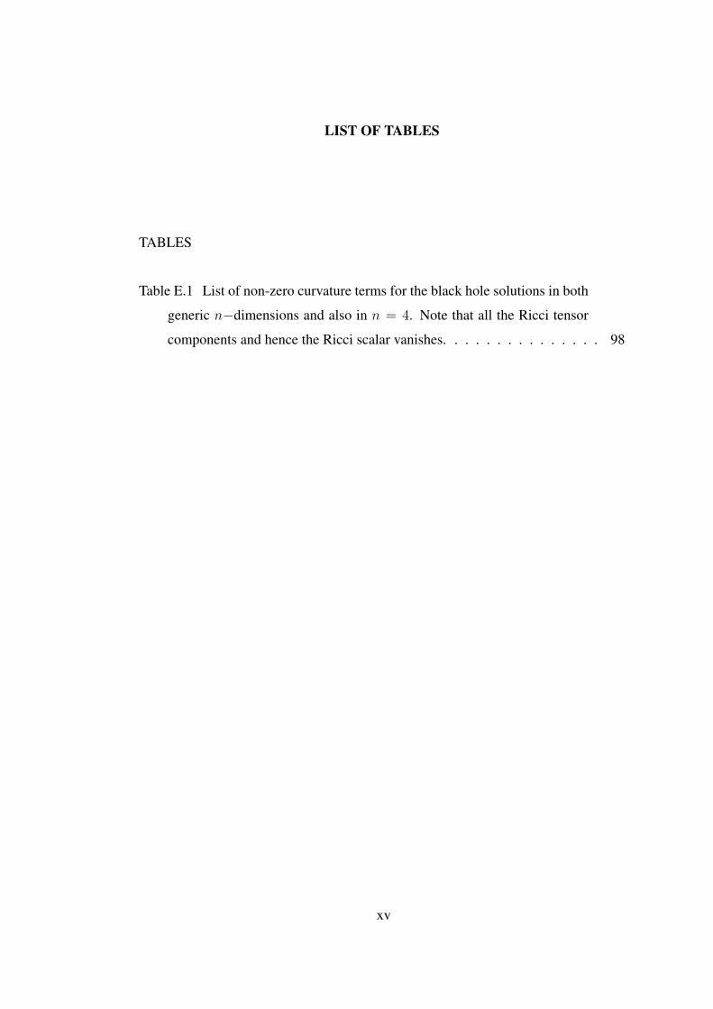
Table E.1 List of non-zero curvature terms for the black hole solutions in both
generic n−dimensions and also in n = 4. Note that all the Ricci tensor
components and hence the Ricci scalar vanishes. . . . . . . . . . . . . . . 98
xv

LIST OF FIGURES
FIGURES
Figure 1.1 Tree-level scattering amplitude between two sources . . . . . . 13
xvi

LIST OF ABBREVIATIONS
GR General Relativity
EH Einstein-Hilbert
BI Born-Infeld
RN Reissner-Nordström
ηµν Mostly plus Minkowski metric (−+ + + . . .)
gµν Generic metric
dΩ22 Line element on unit sphere
g Metric determinant
∂µ Partial derivative
∇µ Metric compatible covariant derivative
Fµν Electromagnetic field tensor
L Lagrangian density
NOTATION: Latin indices ijk run from 1 to (D− 1) and Greek indices µνρ
run from 0 to D. We follow Einstein’s summation convention,
i.e. uµvµ =
D∑µ=0
uµvµ and use units kB = c = 1 throughout
the text.
xvii

xviii

CHAPTER 1
INTRODUCTION
The life we experience may have surprises for us but to see an apple falling from a
tree is not one of them thanks to Isaac Newton. He thought that there was a force
which was responsible for this attraction between the apple and the Earth. In 1687 he
wrote his gravity theory that would last for centuries and formulated this force as [1]
F = −Gm1m2
r2, (1.1)
where the minus sign shows that the force is attractive, G is the Newton’s constant
and r is the distance between the two masses m1 and m2. Applying this equation
to the Newton’s laws of motion determined the orbits of the heavenly objects around
the Sun, the tidal forces of the Moon and even the mass of the Sun and the Earth [2].
The discovery of the planet Neptune whose location was predicted by the unexpected
perturbations of the orbit of Uranus was another success of the Newton’s theory of
gravity [3, 4]. In the beginning of the 20th century, the same approach was intended
to explain the perihelion precession of Mercury that was larger than the expectations
of the Newton’s gravity. As in the case of the discovery of Neptune, people searched
for a new planet named Vulcan which was never observed. Fortunately, this problem
was cured by a remedy found by Einstein. In 1915 he proposed the theory of General
Relativity [5] and showed that the discreapency in Mercury’s orbit could be explained
not by looking for a new planet but looking for a new theory.
General Relativity is a theory of space, time and gravitation. As John Wheeler said,
"Space-time tells matter how to move; matter tells space-time how to curve" [6]. The
spacetime and the matter are related via Einstein’s equations
Rµν −1
2Rgµν = κTµν , (1.2)
1

where κ is some constant and Tµν is the all the source that can be in the form of
energy, momentum, pressure and stress of the matter. The left hand side contains the
Ricci tensorRµν , the Ricci scalarR and the metric gµν which determine the geometry
of the spacetime.
After successfully explained the perihelion precession of Mercury, the theory of Gen-
eral Relativity immediately was tested for the phenomena such as the light bending
and the gravitational redshift that could not be understood by Newton’s gravity. Pass-
ing these two tests proved that the General Relativity was successful to explain the
phenomena within the solar system [7, 8] but out of this scale the theory is inadequate
to explain the "cosmological constant problem" that is still unsolved. Einstein was the
first person who speculated the existence of this constant. In 1917, to have a static
universe he included the cosmological constant term Λ to his equations (1.2)
Rµν −1
2Rgµν + Λgµν = κTµν , (1.3)
that can be considered as the simplest modification of the General Relativity [9, 10].
In 1922, Friedmann showed that there are two fates of the universe; either contracting
or expanding but not static [11]. In 1929, Hubble showed that our universe is not
contracting [12]. In fact in 1998 it was proved that our universe is expanding with an
acceleration. As we know from the Newton’s laws of motion, if there is an acceler-
ation then there should be some mass-energy in the environment. Today, we named
this energy as dark energy that is considered to be the 70% of the universe’s energy.
We started with the cosmological constant problem and ended with the dark energy.
The relation between them is that the cosmological constant Λ is considered as the
simplest form of the dark energy [10].
One can study the cosmological constant problem starting from its quantum field
theory origin. From the quantum field theory perspective, the vacuum energy density
is not zero. It follows from the fact that the processes of annihilation and creation
occur with pairs and occur at any time. Therefore the universe will have an energy
density even if there was nothing in it. If we apply this situation to General Relativity,
we reach the idea that it does not matter whether there is an energy distribution in the
universe, the existence of cosmological constant will lead to a curvature. The idea of
these two theories relate the cosmological constant and the vacuum energy density of
2
the universe. Although this relation warms our hearts, at the end of the day it turns
to a nightmare. Since we expect to obtain rather close values for the cosmological
constant, it should not be really important which theory we use. However this is not
true, in fact the values coming from the observation and the quantum field theory are
not close but differs with 10−122 (in Planck units) and (∼ 10−2) respectively. The
predictions of the theory and the observation do not match. This inconsistency is
known as cosmological constant problem. In the other extreme, to understand the
gravity in very small scales, one should consider the quantum effects. Unfortunately,
no consistent theory of quantum gravity has been written so far [10].
General Relativity is mandatory to understand the physics of the black holes including
their thermodynamics. In 1969, Penrose showed that it was possible to extract the
rotational energy of the Kerr black hole that had an angular momentum. This process,
known as Penrose process, depends on the existence of the ergosphere that is the
region between the stationary limit and the outer event horizon of the Kerr black hole.
In this process, he considered a particle with energy E1 that was sent from infinity.
It entered the ergoregion and then splitted into two pieces with energies E2 and E3
respectively such that the energy of the second particle, as measured by the observer
at infinity, is negative and absorbed by the black hole. However, the third particle with
the energy E3 escapes to infinity. By using the conservation of the energy and the fact
that the energy of the second particle is negative, one can conclude that E3 > E1 that
means the energy of the third particle is bigger than the energy of the original particle.
This extra energy is extracted from the black hole’s rotational energy [13]. In 1971,
Penrose and Floyd suggested that the surface area of the event horizon may naturally
increase in time [14]. In 1970 independently, Christodoulou derived the mass-energy
of a rotating black hole with angular momentum such that
m2 = m2ir +
L2
4m2ir, (1.4)
where m is the mass-energy, mir is the irreducible mass and L is the angular momen-
tum of a black hole. Although it was possible to increase or decrease the mass of
a black hole or its angular momentum as shown by Penrose, it was not possible to
decrease mir by any kind of processes. It can be only increased by irreversible trans-
formations or does not change by reversible transformations [15]. In 1971, Hawking
3

proved that the area of the event horizon never decreases which is given by
AH = 8πm[m+ (m2 − a2)1/2
], (1.5)
where AH is the area of the event horizon, m is the mass and a is the angular momen-
tum per unit mass. If one considers the merging of two black holes with parameters
m1, a1 and m2, a2 that formes a single black hole with parameters m3, a3, the surface
area after merging should satisfy the inequality [16]
m3
[m3 + (m2
3 − a23)1/2
]> m1
[m1 + (m2
1 − a21)1/2
]+m2
[m2 + (m2
2 − a22)1/2
].
(1.6)
In 1971, Christodoulou and Ruffini generalized their ideas for charged black holes
and obtained the result
m2 =(m2
ir +e2
4m2ir
)2+
L2
4m2ir, (1.7)
where m is the mass-energy, mir is the irreducible mass and L is the angular momen-
tum and e is the electric charge of the black hole. They also pointed out the one-to-one
connection between the mir and the proper surface area of the event horizon which
was a nondecreasing quantitiy shown by Hawking [16] such as
A = 16πm2ir, (1.8)
where A is the surface area of the event horizon [17].
In 1972, Bekenstein proposed that a black hole must have entropy, otherwise it would
violate the second law of thermodynamics. One can understand this violation by the
following example. Consider an observer throwing a particle into a black hole. When
the particle crosses the event horizon, since it never comes back and carries entropy,
the entropy of the exterior universe decreases hence the violation of the second law.
To prevent this, Bekenstein considered that black holes must have a finite entropy
and stated the second law as " Common entropy plus the black hole entropy never
decreses". Common entropy stands for the entropy of the exterior universe and the
black hole entropy is given by
SBH = η L−2P A, (1.9)
LP is the Planck’s length that are for dimensional considerations, A is the surface
area of a black hole and η is a constant of order unity [18]. The relation between the
4

black hole entropy SBH and the area of a black hole A follows from the conclusions
of Christodoulou [15, 17] and the Hawking [16, 19].
In 1973 Bardeen, Carter and Hawking wrote the thermodynamic-like expressions for
the stationary axisymmetric solution of the Einstein equations. By using the analogy
between the surface area A and the surface gravity κ of the event horizon with the
entropy and temperature respectively, they postulated the four laws of black hole
mechanics as follows [20]:
The Zeroth Law: For a stationary black hole, the surface gravity κ is constant on the
event horizon.
The First Law: δM = κ8πδA+ ΩδJ ,
where M is the mass, A is the surface area, Ω is the angular velocity and the J is
the angular momentum of a rotating black hole. They emphasized that the relation
between the surface gravity and the temperature is nothing but an analogy. If a black
hole has a temperature, it must also emit rediation, which is classically impossible
[20]. However as we are going to see, a black hole has a temperatue T =~κ2π
and it
emits Hawking radiation [21].
The Second Law: The surface area of an event horizon is a non decreasing quantity,
i.e δA ≥ 0.
This states that if two black holes with surface areas A1 and A2 merge, then the final
black hole with surface area A3 satisfies the relation
A3 > A1 + A2. (1.10)
We should note that this law is a bit stronger than the second law of the thermody-
namics because one can transfer entropy between two systems that cannot be done by
the areas.
The Third Law: It is not possible to reduce the surface gravity κ to zero by finite
number of processes.
If it was possible, then creating a naked singularity by carrying these processes would
be also possible [20].
5

In 1975, Hawking showed that a black hole could emit radiation due to the vacuum
quantum fluctuations near the event horizon and defined the entropy of a black hole
as
SBH =A
4G~, (1.11)
where A is the area of the event horizon, ~ is the Planck’s constant and G is the
Newton’s constant [21].
We should emphasized that all the four thermodynamic-like laws for black holes are
derived from Einstein’s equations and it was thought that the relation between the
laws of thermodynamics and the laws of black hole mechanics are nothing but an
analogy. However, the Hawking radiation showed that this was not an analogy but an
identity [20, 21].
Although General Relativity has built a kingdom within the solar system scale, one
should understand the phenomena in very small or large distances; therefore, GR
needs some modifications. One should keep in mind that the modified theory should
reduce to the Einstein’s theory when it is treated in solar system scales. The General
Relativity is a theory with a massless spin-2 excitation and there are different ways to
modify it. We already discussed the simplest modified gravity theory (1.3). Another
way is to give mass to the graviton that is known as massive gravity. The basic idea
is to change the degrees of the freedom of the theory [10].
The electron’s discovery in 1897 by Thompson and the inconsistency of the Maxwell
theory at the atomic scale led people to seek a new theory of electrodynamics in
which the self energy of charged particles was finite at short distances. One of the
attempts was to generalize the Maxwell theory nonlinearly. The idea was to introduce
a maximal field to remove the inconsistency issue [22].
Mie was the first person to develope such a model by assuming that there was a
maximum electric field E0 such that the force was proportional to
F ∼ E√1− E2
E20
. (1.12)
Although this model was promising to solve the issue of infinite energy, it was not
acceptable because it was not covariant under Lorentz transformations [22, 23]. In
6

1932 Born, then in 1934 Born and Infeld proposed a new theory of electrodynamics
with the following Lagrangian
LBI := −b2
(1−
√−det(ηµν +
1
bFµν)
), (1.13)
where ηµν is the Minkowski metric, Fµν is the electromagnetic field tensor. The
dimensionful constant b accounts for the maximal electric field E0 as in Mie’s theory
of electrodynamics [22]. Also, b is called as an absolute field by the originators of the
BI theory. As we are going to study later, b is a measure of nonlinearity and when it
goes to infinity, LBI reduces to linear Maxwell theory with LM [24, 25].
Because of the nonlinear feature of the theory, it is very difficult to analyze and solve
the fields equations. Some attempts concerning this issue were made by Pryce [24,
26]. However, the progress in Quantum Mechanics, Dirac’s contributions on classical
electron and the studies on quantum field theory caused BI theory to be forgotten for
a long time [22, 24, 26, 27].
Since 90’s, there has been a renewed interest in BI nonlinear electrodynamics due to
the research on String Theory. It was understood that D-branes with low energy can
be described from a BI type action. The advent in string dualities conducted a de-
tailed investigation on duality of BI theory [24, 28]. Also, nonlinear electrodynamics
have been studied in gravity to study and understand the feature of regular black hole
solutions [29].
Let us explain what we mean by the inconsistency in Maxwell electrodynamics. As
we are going to discuss in detail, the energy of a charged point like particle is infinite
for large fields or at small distances [30]. It was Born’s motivation to generate a
theory of electromagnetism such that the self energy of a point charge at origin is
finite [24]. We will show that, this is not an issue in BI electrodynamics.
Although BI theory is a nonlinear theory, it has special properties that not all the
nonlinear theories have. To understand what makes the BI theory special, let us first
discuss the feature of nonlinear theories of electrodynamics. As we are going to study,
the dynamics of this kind of theories arise from an action in the form:
S =
∫dDxL(Fµν) +
∫dDxAµj
µ, (1.14)
7
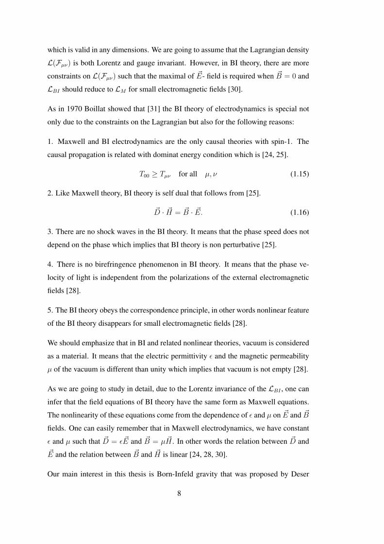
which is valid in any dimensions. We are going to assume that the Lagrangian density
L(Fµν) is both Lorentz and gauge invariant. However, in BI theory, there are more
constraints on L(Fµν) such that the maximal of ~E- field is required when ~B = 0 and
LBI should reduce to LM for small electromagnetic fields [30].
As in 1970 Boillat showed that [31] the BI theory of electrodynamics is special not
only due to the constraints on the Lagrangian but also for the following reasons:
1. Maxwell and BI electrodynamics are the only causal theories with spin-1. The
causal propagation is related with dominat energy condition which is [24, 25].
T00 ≥ Tµν for all µ, ν (1.15)
2. Like Maxwell theory, BI theory is self dual that follows from [25].
~D · ~H = ~B · ~E. (1.16)
3. There are no shock waves in the BI theory. It means that the phase speed does not
depend on the phase which implies that BI theory is non perturbative [25].
4. There is no birefringence phenomenon in BI theory. It means that the phase ve-
locity of light is independent from the polarizations of the external electromagnetic
fields [28].
5. The BI theory obeys the correspondence principle, in other words nonlinear feature
of the BI theory disappears for small electromagnetic fields [28].
We should emphasize that in BI and related nonlinear theories, vacuum is considered
as a material. It means that the electric permittivity ε and the magnetic permeability
µ of the vacuum is different than unity which implies that vacuum is not empty [28].
As we are going to study in detail, due to the Lorentz invariance of the LBI , one can
infer that the field equations of BI theory have the same form as Maxwell equations.
The nonlinearity of these equations come from the dependence of ε and µ on ~E and ~B
fields. One can easily remember that in Maxwell electrodynamics, we have constant
ε and µ such that ~D = ε ~E and ~B = µ ~H . In other words the relation between ~D and~E and the relation between ~B and ~H is linear [24, 28, 30].
Our main interest in this thesis is Born-Infeld gravity that was proposed by Deser
8
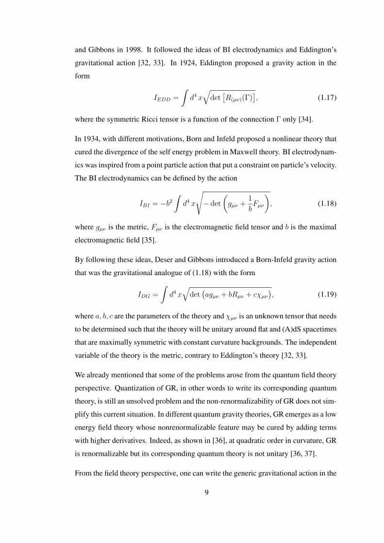
and Gibbons in 1998. It followed the ideas of BI electrodynamics and Eddington’s
gravitational action [32, 33]. In 1924, Eddington proposed a gravity action in the
form
IEDD =
∫d4 x
√det[R(µν)(Γ)
], (1.17)
where the symmetric Ricci tensor is a function of the connection Γ only [34].
In 1934, with different motivations, Born and Infeld proposed a nonlinear theory that
cured the divergence of the self energy problem in Maxwell theory. BI electrodynam-
ics was inspired from a point particle action that put a constraint on particle’s velocity.
The BI electrodynamics can be defined by the action
IBI = −b2
∫d4 x
√− det
(gµν +
1
bFµν
), (1.18)
where gµν is the metric, Fµν is the electromagnetic field tensor and b is the maximal
electromagnetic field [35].
By following these ideas, Deser and Gibbons introduced a Born-Infeld gravity action
that was the gravitational analogue of (1.18) with the form
IDG =
∫d4 x
√det(agµν + bRµν + cχµν
), (1.19)
where a, b, c are the parameters of the theory and χµν is an unknown tensor that needs
to be determined such that the theory will be unitary around flat and (A)dS spacetimes
that are maximally symmetric with constant curvature backgrounds. The independent
variable of the theory is the metric, contrary to Eddington’s theory [32, 33].
We already mentioned that some of the problems arose from the quantum field theory
perspective. Quantization of GR, in other words to write its corresponding quantum
theory, is still an unsolved problem and the non-renormalizability of GR does not sim-
plify this current situation. In different quantum gravity theories, GR emerges as a low
energy field theory whose nonrenormalizable feature may be cured by adding terms
with higher derivatives. Indeed, as shown in [36], at quadratic order in curvature, GR
is renormalizable but its corresponding quantum theory is not unitary [36, 37].
From the field theory perspective, one can write the generic gravitational action in the
9

form
I =
∫d4 x
1
κ(R− 2Λ0) +
∞∑2
anRiem, Ric, R,∇Riem...n. (1.20)
As seen from the (1.20), the first term leads us to Einstein’s gravity, the second term
is its extension with cosmological constant and the rest stands for the higher order
curvature terms. The main interest is to determine which curvature terms appear at
which order and with which couplings [33].
BI type gravity theory is a higher curvature theory at infinite order with fixed cou-
plings and it is a modification of General Relativity. The aim is to determine the
order of n and the corresponding coefficients an in general. Also, by putting the
constraints on (1.20) we will have a consistent theory whose spectrum is ghost and
tachyon free. When we increase the number of these constraints, we can have a spe-
cific theory. The scope of the thesis [33] we have been using as a guide was to obtain
a unitary theory around flat and (A)dS backgrounds that are maximally symmetric
spacetimes with constant curvature.
In three dimesions, there are two, worth-mentioning, examples of BI gravity. The first
one is the BI extension of new massive gravity with the action [38]
IBINMG = −4m2
κ2
∫d3 x
[√− det
(gµν −
1
m2Gµν
)−(
1− λ0
2
)√−g], (1.21)
that is the first example of BI gravity which is unitary around (A)dS spacetime. The
second example is, at quadratic order, the expansion of (1.21) in curvature that leads
the new massive gravity (NMG) theory in the form [39, 40]
INMG =1
κ2
∫d3 x√−g[−R− 2λ0m
2 +1
m2
(RµνR
νµ −
3
8R2
)], (1.22)
that is the unique gravity theory at quadratic order which is unitary around both flat
and (A)dS backgrounds. Both theories have massive spin-2 particle[41, 42, 43, 44].
A detailed explanation is provided in [33].
1.0.1 Unitary Analysis of Born-Infeld Gravity
A gravity theory is physically consistent at the tree level if its spectrum does not
contain any ghosts and tachyons. A ghost is a negative kinetic energy mode that is
10

described by an action
I =
∫dt(−K − U), (1.23)
where K and U are the kinetic and potential energies, respectively. The corresspond-
ing energy mode H = −K + U is not positive definite and this leads to an unstable
vacuum. Ghost instability can be considered as a plauge that is seen at all energy
scales. Nothing is sunny in the corresponding quantum theory either. In the Hilbert
space, a ghost mode has a negative norm that violates the conservation of probability
and leads to a non-unitary theory.
Tachyons are the negative m2 modes that are encountered at energy scales approach-
ing to m. To understand tachyon instability let us consider the following action with
a scalar field φ such that
I[φ] =
∫dt[K(∂µφ)− U(φ)
]. (1.24)
Considering the fluctuations around the vacuum φ with φ− φ ≡ ψ, then the perturbed
action yields[dUdφ
]φ
= 0 for vacuum and[d2Udφ2
]φ
= m2 for squared mass. Therefore
if there is a tachyon, then unstable vacuum occurs at[d2Udφ2
]φ
< 0 [33].
As we mentioned before, the main interest in the thesis [33] that we use as a guide
was to do the analysis of the spectrum and check its unitarity in higher curvature
theories. To carry the calculations further, it is necessary to specify the corresponding
free theory that solves the field equations of these higher order curvature theories.
Also, this free theory is given by the action that is second order in metric fluctuations
around flat and (A)dS backgrounds. As we are going to see, the unitarity analysis
around different backgrounds leads different solutions in principle. Let us discuss
how the features of the free theory differ around flat and (A)dS backgrounds by the
following observations [33]:
Observation 1: For flat spacetime, there is no contribution beyond quadratic curva-
ture terms. For (A)dS spacetimes, all terms contribute in principle.
11

To understand it better, let us find out the contributions coming from R3 term. The
expansion of Ricci scalar in terms of metric fluctuations is given by
R = R +R(1) +R(2) + ... (1.25)
which are the background curvature, first order in curvature and second order in cur-
vature respectively. Then the second order contributions of R3 are found as RR2(1)
and R2R(2). As immediately seen, they both vanish in flat but survive in (A)dS back-
grounds in principle.
Observation 2: Contributions beyond the quadratic order are in the same form as
the contributions from the quadratic order in (A)dS background. They differ with
an overall R factor. To understand it better, let us examine the contributions coming
fromR2 andR3. The contributions from former areR2(1) and RR(2). Comparing these
by the contributions coming fromR3 reveals us that they have the same structure with
the exception of R factor.
Following these two observations, we can conclude that the structure of the most
general quadratic action can be determined by the scalars R2, RµνR
νµ and Rµν
ρσRρσµν .
Instead of the last term, we can use the Gauss-Bonnet combination that is valid for
D > 4.
Following these ideas, one can write the most generic theory at quadratic curvature in
the form of
I =
∫dD x√−g[1
κ(R− 2Λ0) + αR2 + βRµ
νRνµ + γRµν
ρσRρσµν
]. (1.26)
The unitary analysis of (1.26) gives us a hint about the unitarity of higher order cur-
vature theories. They will be unitary if and only if its propagator can be reduced to
a propagator of a unitary theory that has already been determined. Therefore, the
unitary analysis of (1.26) is rather essential [33].
Let us finalize this section by discussing the unitary analysis of Born-Infeld type
gravity theories that can be obtained by analyzing tree level amplitude.
12

Figure 1.1: Tree-level scattering amplitude between two sources
The tree level amplitude given by Feynmann diagram (1.1) is defined as
A =
∫dD x√−g T ′µν(x)hµν(x), (1.27)
where the metric fluctuaton hµν is given by hµν ≡ gµν − gµν and created by the
matter Tµν . To determine the unitarity of (1.26), we should reduce it to a propagator
whose unitarity is known. But this is not trivial since the differential operator Oρσµνthat represents the matter Tµν in such a way that Oρσµν hρσ = Tµν involves fourth
and second derivatives therefore Oρσµν has a complex form. Also, it is not possible to
invert Oρσµν directly. Following the steps studied carefully in [33], one can obtain the
amplitude in the desired form of
A
κe= 2T ′µν
[(κeβ + 1)(∆
(2)L −
4Λ
D − 2)]−1
T µν
+2
D − 2T ′[(κeβ + 1)( +
4Λ
D − 2)]−1
T
− 2(β + c)
c(D − 1)(D − 2)T ′[(κeβ + 1)(−m2
s)]−1
T (1.28)
+8ΛDβ
c(D − 1)2(D − 2)2
xT ′[(κeβ + 1)(−m2
s)( +2ΛD
(D − 1)(D − 2))]−1
T,
where ∆(2)L is the symmetric rank-2 Lichnerowicz operator; c ≡ 4(D−1)α+Dβ
D−2and the
scalar excitation mass will be
m2s =
1
cκe− 2ΛD
(D − 1)(D − 2)
(1− β
c
). (1.29)
13

Some properties of the ampilute (1.28) can be discussed as follows [33]:
• When α = β = γ = 0 one part of (1.28) produces the amplitude of GR that is
unitary.
• Pole (κeβ + 1)−1 stands for the massive spin-2 excitation which couples to
the sources in tensorial form.
• Pole ( −m2s)−1 stands for the massive spin-0 excitation that couples only to
the trace of a source.
• These poles are multiplied with each other in the amplitude. This feature of the
amplitude implies the excistence of ghosts that leads to a non-unitary theory.
In fact, the unitarity of massive spin-2 conflicts with the unitarities of massive
spin-0 and massless spin-2 excitations. Therefore removing the massive spin-2
mode from the spectrum by taking β = 0 gives us a unitary theory.
If we carry these procedures carefully, we will obtain the unitarity analysis of (1.26)
as follows [37, 39, 43]:
• For D = 4, GR is a unitary theory around flat and the (A)dS backgrounds. It
has a massless spin-2 excitation. Its R2 extension is not renormalizable as GR
but unitary with another spin-0 excitation. To cure non-renormalizability, one
can addRµνR
νµ that costs to lose unitarity due to new massive spin-2 ghost mode
in the spectrum.
• For D = 3, GR has no propagating excitations. Its R2 extension is still unitary
with a massive spin-0 mode. But a generic extension of αR2 + βRµνR
νµ costs
an additional massive spin-2 mode to spectrum that spoils the unitarity due the
the conflict between these two modes. This conflict can be solved by the proper
choice of the parameters such that 8α+3β = 0 which gives the NMG case [39].
This choice of parameters removes the massive spin-0 mode from the spectrum
hence the resulting theory with massive spin-2 excitation will be unitary around
flat and (A)dS backgrounds.
• For D > 4 Gauss-Bonnet (GB) term is valid. Both GR and its GB extensions
are unitariy around the flat and (A)dS backgrounds with massless spin-2 exci-
14
tations. The R2 extension of both theories do not spoil their unitarities and add
massive spin-0 mode to spectrum. However the RµνR
νµ extension of the theory
results a ghost term to the spectrum that is a massive spin-2 excitation therefore
leads a non-unitary theory.
The layout of this thesis is as follows: In the next chapter, we discuss the black hole
thermodynamics in detail and calculate the corresponding thermodynamic quantities
for a generic metric. The chapter three that is the bulk of this thesis is devoted to show
how we calculated the Wald entropy for Born-Infeld type gravity theories. We discuss
the Wald entropy of both n-dimensional and three-dimensional Born-Infeld theories
and show that this dynamical entropy reduces to the geometric Bekenstein-Hawking
entropy with the appropriate choice of effective gravitational constant. A conclusion
chapter is followed by appendices that give related calculations with the chapters. We
should note that the figure (1.1) in this chapter is taken from [33].
15

16
CHAPTER 2
BLACK HOLE THERMODYNAMICS
1 Classical mechanics perfectly describes the motion of a particle or the orbits of heav-
enly objects around the Sun. But when the system we are interested in involves heat
exchange also, Newton mechanics will be insufficient because it does not know how
to read the coordinates of the thermal systems. Therefore to have a complete descrip-
tion, we need to define thermal properties of the system besides the mechanical ones;
which is the scope of Thermodynamics. Although these two theories figure different
parts of the same system, they have common features also. First of all, mechanical
and thermal descriptions are nothing but idealizations. In classical mechanics, we use
point particles which are the mechanical counterparts of closed systems in Thermo-
dynamics. Such systems are separated from surroundings by adiabatic walls which
do not allow heat exchange. Secondly, in classical mechanics the state of a particle
is given by its momentum and position whereas in Thermodynamics, we describe the
macroscopic systems by state functions that can be mechanical and thermal. As we
know, pressure and volume are mechanical state functions for a gas; and for the ther-
mal systems we have thermodynamic state functions like temperature for example.
These state functions are well defined only in equilibrium when the properties of the
system do not change anymore. Final similarity between Newtonian mechanics and
Thermodynamics is that both theories depend on basic observations and laws; then a
mathematical structure is constructed by using them.
One can easily conclude that Thermodynamics is valid only in equilibrium and de-
scription of the macroscopic system relies on the observations. This means that we
obtain thermodynamic laws from observations.
1 This section is based on [45].
17
The zeroth law shows the transitivity property of equilibrium and defines the thermal
state function- the emprical temperature Θ such that
ΘA(A1, A2, ...) = ΘB(B1, B2, ...) = Θ, (2.1)
where A and B are two systems in equilibrium with each other.
The first law shows what kind of transformations we can have. In adiabatically iso-
lated systems, the work done to transform a state depends only on initial and final
points. When we remove this constraint and consider the transformations that also
involves heat, then the previous result will no longer be true. Hence in general, for
infinitesimal changes, one can write the first law as
dE = dW +dQ, (2.2)
where dW and dQ are the increment work done on the system and heat put into the
system respectively. Like the zeroth law, the first law generates another state function
E that is known as internal energy. As it is understood from the equation (2.2), to
write down the internal energy, we should find out the mechanical and thermal work
properly. When things are quasistatic in other words slow enough to maintain the
equilibrium, we can describe mechanical coordinates as (Ji, xi) which are generalized
forces and generalized displacements respectively. So one can write
dW = Ji.dxi. (2.3)
Therefore to get the internal energy, one should find out the form of dQ. One can
determine it by using the analogies between Newtonian mechanics and Thermody-
namics. If we use the mechanism of mechanical and thermal equilibrium, one can
infer that generalized forces and the temperature have similar characters. Therefore,
to determine dQ, we only need to find the generalized displacement corresponding to
temperature.
The analog of the generalized displacements come from the second law which indi-
cates the time ordering between transformations. As the Clausius’s theorem states,
one can write the heat as
dQ = TdS, (2.4)
18

for adiabatic transformations and S stands for the another state function called the
entropy.
Third law that is independent from others and concerns the behaviour of the entropy
at low temperature. It reads as
limT→0
S(X,T ) = 0, (2.5)
where X stands for all choice of coordinates.
As this brief discussion shows, the way we approach mechanical and thermal sys-
tems share similarities. Keeping in mind that the mechanical forces are the indicators
of the equilibrium, we determine the place of the temperature T by comparing the
form of dQ and dW . Our main interest in this chapter is the laws of black hole ther-
modynamics and as we will see, we are going to construct some analogies between
thermodynamical systems and the black holes. In order to discuss that black holes
have their own thermodynamic laws, first of all we are going to construct analogies
of macroscopic functions and the notion of equilibrium for the black holes. Then we
also see the relation between thermodynamic entropy and the area of the horizon. We
carry our discussion for generic metrics, then these results for the Schwarzschild, the
charged and the rotating black holes. The detailed discussion in classical thermody-
namics can be found in the Appendix A.
2.1 Thermodynamics of the generic metric
As we studied in the first section of this chapter, we can describe thermodynamic
systems in terms of a few state functions like T, P, V etc. When a system is in thermal
equilibrium with the surroundings, its temperature will remain constant. We can reach
another equilibrium state through transformations and final state will not depend on
the intermediate stages [45, 46].
We have a similar approach in black holes. Black holes can be parametrized through
few parameters likeM,Q and J which stand for mass, charge and angular momentum
respectively. This means that two black holes with same parameters are indistinguish-
able which is known as no-hair theorem. Black holes do not depend on the structure
19

or composition of the initial star. If we consider the merging of two black holes, the
event horizon of the final black hole will be spherically symmetric even though it is
asymmetric through merging. Having a spherically symmetric horizon is an equilib-
rium state for a black hole and it implies that the force per unit mass over the horizon
is constant [46].
We can reach an immediate conclusion that there is a similarity between black holes
and thermodynamic systems. It is clear that the thermal equilibrium and the con-
stant temperature are analogies of spherical symmetry and constant force over hori-
zon which is known as surface gravity. Therefore one can expect to write the zeroth
law for black holes. The main question is whether we can find similar analogies and
write all thermodynamic-like laws for black holes [46].
Let us consider this example. For Schwarzchild black holes, one reads the horizon
area as,
AH = 4πr2H = 16πG2M2, (2.6)
whereG is the Newton’s constant andM is the mass of the black hole. It is easy to see
that horizon area is proportional to mass square of the black hole. Classically, nothing
can escape from a black hole therefore mass is a nondecreasing quantity which leads
us an important result
4A ≥ 0, (2.7)
that has the similar property with the thermodynamic entropy S. Hence one can
expect that black holes have entropy.
Actually black holes obey all thermodynamic-like laws and we are going to obtain
these for generic black holes, then we are going to check them for two black holes
Schwarzschild and Reissner-Nordström that are written in the same form of the metric
[46].
2.1.1 The Zeroth Law
As the zeroth law of thermodynamics suggests, a thermal equailibrium can be given a
constant temperature. In the context of black holes no matter how the inital collapse,
20
the black hole will have a horizon at r = constant also suggest the gravitational force
on the horizon is constant. Therefore if we consider rH = constant as the equilibrium
state, one can consider the gravitational force on the horizon as the temperature. If
we define the gravitaional force or the gravitational acceleration on the horizon as the
surface gravity, we can state the zeroth law for black holes as [20, 46]:
Zeroth Law: For a stationary black hole, the surface gravity κ is constant on the
event horizon.
By definition, the surface gravity is the gravitational acceleration that is necessary to
stay at the horizon. In Newtonian mechanics, the gravitational acceleration is
a =GM
r2. (2.8)
At the Shwarzschild horizon, we obtain the surface gravity (2.8) as
κ = a(r = rH) =1
4GM. (2.9)
Although it seems that one can calculate the above result by using the Newtonian the-
ory, it is not the case actually. In General Relativity, we have to specify who measures
the quantity. For an infalling observer, surface gravity diverges because irrespective
of the strength of the force, his/ her fate is to pass the horizon and reach the singular-
ity. But if the asymptotic observer measures it, it will not diverge and gives the result
(2.9). The disagreement in the accelerations occurs due to the gravitational redshift
[46].
Surface Gravity
Let us give the proper definition. The surface gravity is the gravitational acceleration
that is necessary to hold the particle at the horizon by an observer at infinity. One can
write the static metric as
ds2 = −f(r)dt2 +dr2
f(r)+ r2dΩ2. (2.10)
The particle’s motion is discussed in detail in Appendix C, so following these steps
one can have (drdτ
)2= E2 − f(r) + L2 f
r2. (2.11)
21
We carry our calculations without angular momentum since our particle falls radially.
If we take the derivative of the equation (2.11) with respect to τ then we get
d2r
dτ 2= −1
2
∂f
∂r= −GM
r2= ar, (2.12)
that is the familiar Newtonian acceleration. However we only have the r-component
of the acceleration, it is not in the covariant form aµ. One can read its magnitude as
a2 = grrarar =
f ′2
4f=⇒ a =
f ′
2√f, (2.13)
where f ′ = ∂r. It can be easily captured that the above result diverges for an infalling
observer as promised.
To calculate surface gravity as measured by the asymptotic observer, consider she/ he
is connected to a particle at r by a massless string. If she/ he pulls the string by a
proper distance δs [46], the work done by observer and work done on the particle are
given by
W∞ = a∞δs and Wr = aδs. (2.14)
One can convert Wr to radiation energy Er and it can be received by the asymptotic
observer. If we use the gravitational redshift formula
E∞ =
√f(r)
f(∞)Er. (2.15)
Since the metric is asyptotically flat, f(∞) = 1. If we apply the conservation of
energy to the equation (2.15) and use the equation (2.13) later, then we obtain the
result
κ = a∞(rH) =f ′(rH)
2, (2.16)
which coincides with (2.9) for the Schwarzschild black hole [46].
2.1.2 The First Law
We already disccussed that the horizon area and the black hole’s mass-square are
proportial. Since the change in mass can only be positive, any change in black hole’s
mass increases the horizon area. Therefore we can start with the equation
dM ≈ dA, (2.17)
22

and by using dimensional analysis we can obtain the first law. We should add the
Newton’s constant G to the left hand side of the equation since we have G in a com-
bination with mass in GR. Then we should add a quantity with dimension of accel-
eration to the right hind side of the equation to make them dimensionally equivalent.
We can use surface gravity κ as an acceleration. If we differentiate the equation (2.6)
and also apply the surface gravity equation (2.9), we can read the first law of black
hole thermodynamics asκ
8πdA = GdM, (2.18)
for the Schwarzschild black hole. In the general form, it can be written as
dM =κ
8πdA+ ΩdJ + ΦdQ, (2.19)
where E is the mass/energy, Ω is the angular velocity, J is the angular momentum, Φ
is the electrostatic potential and Q is the electric charge [20, 46].
2.1.3 The Second Law
We should stress that we haven’t derived these black hole laws.We constructed analo-
gies between classical systems and thermodynamic ones and now we are trying to
extend these thermodynamic laws to black holes. Actually, if we take a look on these
black hole laws, we can see that there are some problems. First of all, when we write
thermodynamic laws for black holes that means we consider them as thermal sys-
tems. But a thermal system has temperature and emits radiation. However nothing
can escape from a black hole, so how can this happen? Secondly, the units of area and
the entropy do not match. The entropy is dimensionless but we still have a dimen-
sionful area. Let us explain these issues carefully and discuss the solutions that leads
us to the second law of black holes known as the area theorem [46]. We know that
the black holes are created from a gravitational collapse that includes huge amount of
matter. We also know that the matter obeys quantum mechanics. If we consider black
holes quantum mechanically, we can see that the black holes emit radiation known as
Hawking radiation with the temperature [21, 49]
T =~κ2π. (2.20)
23
We should emphasize that this is not a classical result which is clear due to the ~. The
Hawking temperature is related with the surface gravity so using this relation in the
equation (2.18), we can rewrite the first law of the Schwarzschild black holes as
dM =κ
8πGdA = T
1
4G~dA. (2.21)
Using the fact that the surface gravity is the analog of the temperature, if we compare
the first law of thermodynamics dE = TdS with the above equation, we obtain
SBH =AH4G
1
~=AH4L2
p
, (2.22)
which is the Bekenstein-Hawking entropy [21, 46]. One should notice that we have
given solutions to the issues we pointed out initially. We have temperature for the
Schwarz-schild black holes now. We also clarify the point that the entropy is dimen-
sionless whereas the area is not. We divided the area by Plank length square L2p hence
the equation (2.22) is dimensionless now [46]. After all these calculations, we still
did not derive the entropy. The basic reason is that microscopically, entropy is the
measure of the degrees of the freedom of the system but we have not counted any
states. But still the laws we obtain are considered as black hole laws. Another impor-
tant thing is as the equation (2.22) shows, the black hole entropy depends on the area
while the statistical entropy depends on the volume. This reveals that a black hole
cannot have a statistical interparation at the same dimensions. However, since area in
five dimensions is the volume in four dimensions, the five dimensional black hole can
have a statistical interpretation in the four dimensional spacetime. That is the scope
of the theory known as AdS/CFT. It basically states that the black holes can have a
statistical description in the spacetime that has one dimension lower than the space-
time the gravitational theory lived. Before the derivation of the Hawking temparature,
we should note that although we carried our calculations for the Schwarzschild black
hole, the area theorem (2.22) is valid for all black holes as long as they are described
by Einstein-Hilbert action
SEH =1
16πGD
∫dD x√−gR, (2.23)
where GD is the Newton’s constant in D-dimensional spacetime, g is the determinant
of the metric and R is the Ricci scalar. For a generic metric, one can find the entropy
by using the Wald entropy formula that we are going to discuss in detail in the next
chapter [46].
24

Hawking Temperature We follow the simplest way to derive the Hawking temper-
ature. The main idea is that assigning a smooth Eucliean spacetime with a periodic
imaginary time tE and assuming that the temperature is the inverse of this periodicity
β. Letting tE = it, then the metric (2.10) takes the form
ds2E = f(r)dt2E +
dr2
f(r)+ ... . (2.24)
Near the horizon r u rH , one can expand the above equation as
ds2E = f ′(rH)(r − rH)dt2E +
dr2
f ′(rH)(r − rH)+ ... . (2.25)
Let us introduce a new coordinate ρ = 2√
(r−rH)f ′(rH)
that puts the above equation in a
simpler form
ds2E = dρ2 + ρ2d
(f ′(rH)
2tE
)2
. (2.26)
It is clear that it looks like the plane polar coordinates if we set the periodicity 2π that
is f ′(rH)2
tE = 2π that leads us
β =4π
f ′(rH)or T =
1
β=f ′(rH)
4π. (2.27)
If we apply the equation (2.16), we obtain the the Hawking temperature as
T =~κ2π, (2.28)
where T = 1/8πGM is the Hawking temperature for the Schwarzchild black hole
[46].
2.1.4 The Third Law
It states that as temperature T approaches to zero, the entropy S aprroaches to some
constant. It is known as Nernst theorem and also states that one can not approach
zero temperature by finite number of transformations [46]. It also states that It is not
possible to reduce the surface gravity κ to zero by finite number of processess [20].
25

2.1.5 The Black hole Thermodynamics for Charged Black Holes
We already showed that for the generic metric in the form (2.10), the thermodynamics
quantities are given as
κ =f ′(rH)
2and T =
~κ2π. (2.29)
The Schwarzschild the Reissner-Nordström metrics have the same form as in (2.10)
but differ with the function f(r). For the former where f(r) = 1 − 2GMr
, the above
quantities are obtained as
κ =1
4GMand T =
1
8πGM, (2.30)
and the first and second laws of thermodynamics are
dM =κ
8πGdA, S =
AH4G
, AH = 4πr2s , (2.31)
where the rs represents the Schwarzschild radius.
The Reissner-Nordström metric describes the spacetime outside the spherical sym-
metric gravitating object that couples to electric field. This means the Einstein equa-
tions are coupled to Maxwell equations
∇µFµν = 0, (2.32)
∇µFνρ +∇ρFµν∇νFρµ = 0, (2.33)
where Fµν is the electromagnetic field strength tensor and the second equation is the
usual Bianchi identity. If one carries a similar approach to determine Schwarzschild
metric carrefully, the Reissner-Nordström solution will be obtained in the form (2.10)
with the function f(r) as
f(r) = 1− 2GM
r+GQ2
r2. (2.34)
It is clear that the solution reduces to Schwarzschild solution in the absence of the
electric charge Q. As it is seen, this f(r) has two roots that are
r± = GM ±√G2M2 −GQ2. (2.35)
The inside of the square root leads us to three different cases. The only physical result
is given fot the case G2M2 > GQ2 where we have the both of r± that are the outer
26

and the inner horizons. Since the asymptotic observer determines the thermodynamic
quantities, one should evaluate the calcuations at r = r+. If we rewrite the function
as f(r) =(r − r+)(r − r−)
r2, one can read the thermodynamic quantities of Reissner-
Nordström black hole as
κ =f ′(r+)
2=r+ − r−
2r2+
and T =~κ2π
=~4π
r+ − r−r2
+
, (2.36)
with the thermodynamics laws
dM =κ
8πGdA+ Φ dQ, S =
AH4G
, AH = 4πr2+ . (2.37)
Detailed calculations can be found in [7].
2.1.6 The Black hole Thermodynamics for Kerr Black holes
2We have discussed the static solutions of Einstein’s equations that are the Schwarz-
schild and Reissner-Nordström black holes. Let us finalize the discussion of the black
holes by introducing the Kerr black holes. Since they are rotating, the Kerr metric is
not static but stationary. In the Boyer-Lindquist coordinates (t, r, θ, φ) the Kerr metric
takes the form
ds2 = −(1− 2GMr
ρ2
)dt2 − 2GMar sin2 θ
ρ2(dtdφ+ dφdt) +
ρ2
4dr2 + ρ2dθ2
+sin2 θ
ρ2
[(r2 + a2)2 − a24 sin2 θ
]dφ2, (2.38)
where M is the energy, J is the angular momentum and a = J/M is the angular
momentum per unit mass. The quantities4 and ρ2 are defined as
4(r) = r2 − 2GMr + a2, (2.39)
ρ2 = r2 + a2 cos2 θ, (2.40)
It is straightforward to see that metric (2.38) reduces to the Schwarzschild metric as
a→ 0.
The metric (2.38) does not depend on the coordinates t and φ which leads the exis-
tence of the Killing vectors K = ∂t and R = ∂φ. As we are going to see K = ∂t is
not null on the event horizon but it is spacelike.2 This subsection is based on [7]
27

The event horizon occurs where grr = 4/ρ2 vanishes. We should note that as in the
Reissner-Nordström metric, there are three possible solutions for4 = r2− 2GMr+
a2. The case GM > a gives physical solution which gives the event horizons as
r± = GM ±√G2M2 − a2, (2.41)
where r+ and r− are the outer and the inner event horizons respectively.
One can easily capture that both horizons are null hypersurfaces. To see this, all
required is to evaluate the normal vector of the hypersurface Σ ≡ r± − a = 0 which
is nµ = (0, 1, 0, 0) at the event horizons r±. Since the norm is grr and it vanishes on
event horizons, we obtain the result that event horizons r± are null hypersurfaces.
We should emphasize that for the other two black holes i.e the Schwarzschild and the
Reissner-Nordström black holes, the Killing vector K = ∂t is null on the event hori-
zon hence event horizon is also the Killing horizon for this Killing vector. However,
this situation is quite different for the Kerr black holes where K = ∂t is not null on
the outer event horizon. Instead it is spacelike there. There is a surface where K = ∂t
is null and this surface is known as the stationary limit surface. Inside this surface,
K = ∂t is spacelike so it is not possible to be static there. A region called the er-
goregion is between the stationary limit surface and the outer event horizon such that
inside this region, it is not possible even for light to move in the opposite direction of
the black hole. We can see this by looking at the trajectory of the light that travels in
the direction φ for the fixed coordinates r and θ and let the motion takes place on the
equatorial plane. If we apply these constraints to the metric (2.38), we have,
dφ
dt= − gtφ
gφφ±√( gtφ
gφφ
)2 − gttgφφ
. (2.42)
On the stationary surface where gtt vanishes, we have two solutions as
dφ
dt= 0
dφ
dt= −2
gtφgφφ
=a
2G2M2 + a2, (2.43)
which shows that the photon is rotating with the black hole inside the ergoregion.
Massive particles are dragged till they reach the outer event horizon. By using equa-
tion (2.43), one can find the angular velocity of the outer event horizon as
ΩH =a
r2+ + a2
, (2.44)
28

which is also the particle’s minimum angular velocity there. As seen, it is slower than
the photon.
We should note that in the ergoregion, it is also possible to extract the rotational
energy of the Kerr black hole by Penrose process [13]. We should emphasize that
although K = ∂t is not zero on the outer event horizon, the linear combination Kµ +
ΩHRµ is zero on the outer horizon and the quantity ΩH is the angular velocity of the
Kerr black hole. We use this combination to calculate the surface gravity κ.
Similarly, one can calculate the angular velocity of the massive particle. One can
determine the stationary limit surface by evaluating KµKµ = 0 and it is given by
(r −GM)2 = G2M2 − a2 cos2 θ. (2.45)
Also, we can rewrite the outer event horizon in terms of
(r+ −GM)2 = G2M2 − a2. (2.46)
The singularity of the Kerr black hole is not r = 0 but it happens where ρ = 0. As
it is seen from the equation (2.40), ρ2 can be zero either when the all terms vanish or
when r = 0 and θ = π/2. Actually this reveals that the singularity is not a point but
a ring [7].
The Killing vectors Kµ = (1, 0, 0, 0) and Rµ = (0, 0, 0, 1) lead us the following
conserved quantities
E = −pµKµ = m
(1− 2GMr
ρ2
)dt
dτ+
2GMmar
ρ2sin2 θ
dφ
dτ, (2.47)
L = −2GMmar
ρ2sin2 θ
dt
dτ+m(r2 + a2)2 −m4a2 sin2 θ
ρ2sin2 θ
dφ
dτ, (2.48)
where m is the mass of the particle.
One can realize that within the ergosphere, the particle can have negative energy
according to observer at infinity. We must emphasize that outside this region, any
particle has positive energy therefore to escape this region to infinity, a particle should
accelerate so has a positive energy. The process to extract energy from a rotating black
hole is known as the Penrose process and basically it depends on the following idea.
Consider a traveler moving along the geodesic and carrying a piece of rock. Outside
29

the Kerr black hole, the initial momentum of the system containing traveler and rock
is given by p(0)µ that leads a conserved positive energy E(0) = −Kµp(0)µ. When they
enter the ergoregion, the rock and the traveler are separated from each other. Now
they carry the four-momenta p(1)µ and p(2)µ that represent the four-momentum of the
traveler and the rock respectively. By the conservation of four momentum, we have
p(0)µ = p(1)µ + p(2)µ, (2.49)
whose contraction with Kµ yields energy conservation
E(0) = E(1) + E(2). (2.50)
It is possible to arrange the trajectroy of the rock such that E(2) < 0. If we apply the
conservation of momentum (2.50), we see that
E(1) > E(0), (2.51)
therefore the energy of the traveler is bigger than the energy of the system containing
the rock and the traveler. This extra energy is extracted from the rotational energy of
the Kerr black hole. Let us show that there is a limit on the extacted energy. To see
this we should use the combined Killing vector χµ = Kµ + ΩHRµ where Kµ and Rµ
are the usual Killing vectors and ΩH is the angular velocity of the Kerr black hole.
The reason why we use χµ is that it is null on the outer event horizon so the surface
r = r+ is a Killing horizon for this Killing vector χµ. We set that the rock passes the
outer event horizon therefore
p(2)µχµ < 0. (2.52)
If we apply the definitions of E and L, we obtain
−E(2) + ΩHL(2) < 0 → L(2) <
E(2)
ΩH
. (2.53)
Since the angular momentum of the black hole ΩH is positive and we set the energy
of the rock as negative, the angular momentum of the rock becomes negative as seen
from the equation (2.53) which shows that it was thrown to move against the rotation
of the black hole. If we set the infinitesimal changes of the black hole as
δM = E(2) and δJ = L(2), (2.54)
30

where J andM are the angular momentum and the mass of the Kerr black hole. Then
we can rewrite the equation (2.53) as
δJ <δM
ΩH
, (2.55)
which shows that there is a limit on extracting the angular momentum of the black
hole.
We should emphasize that we decrease the angular momentum and the mass of the
black hole but we still obey the area law. Let us show that after the Penrose process,
the change in the irreducible mass of the Kerr black hole is positive. Then by using
the relation between the area and the Mir, we also show that the change in area of the
outer horizon is positive also.
To do this, let us start with the definition of the area A that is
A =
∫ √dethijdx
idxj, (2.56)
where hij is the induced metric on the sphere. One can easily capture that dethij =
gθθgφφ = sin2 θ(r2+ + a2)2, then the integral becomes
A = 4π(r2+ + a2). (2.57)
If we use the relation between the square of the Mir and the area [16], we will have
M2ir =
A
16πG2, (2.58)
=1
2
(M2 +
√M4 − (J/G)2
), (2.59)
where the equation (2.59) is obtained after applying the equation (2.57), the definition
of r+ and the equation J = Ma to the equation (2.58). To see that the change in the
Mir is positive after the Penrose process, we should differentiate the equation (2.59)
that gives,
δMir =a
4GMir
√G2M2 − a2
(δM/ΩH − δJ), (2.60)
where we also use the equation J = Ma and the definition of ΩH . If we use the
equation (2.55), we can see that δMir > 0. Differentiating the equation (2.57) and
then using the equation (2.60) gives
δA = 8πGa
ΩH
√G2M2 − a2
(δM − ΩHδJ), (2.61)
31
after rearrenging the terms one can write the equation (2.61) in terms of
δM =κ
8πGδA+ ΩHδJ (2.62)
where we write the surface gravity κ as
κ =
√G2M2 − a2
2GM(GM +√G2M2 − a2)
. (2.63)
It is clear that equation (2.62) is the first law of Kerr black hole. By using these
quantities, we can write the thermodynamics of the Kerr black holes as
T =~κ2π, S =
AH4G
(2.64)
where AH and κ are given in the equations (2.57) and (2.63) respectively.
32

CHAPTER 3
ENTROPY IN BORN-INFELD GRAVITY
3.1 Introduction
1It is perhaps not possible to write a classical theory of gravity that can supersede
Einstein’s gravity in elegance and simplicity, which, in its most succinct form, reads
in the absence of matter as a variational statement
δg
∫Mdnx√−gR = 0. (3.1)
In words, pure general relativity (GR) is a statement about the topological Lorentzian
manifoldM: finding the metrics that are critical points of the total scalar curvature
on the manifold with prescribed boundary and/or asymptotic conditions to model
various physical cases. This statement is valid in generic n−dimensions but trivial
for n = 1 and n = 2. For all other dimensions, pure GR boils down to searching
for solutions of the non-linear partial differential equation Rµν = 0, that is finding
Ricci-flat metrics.
In n = 3, the Riemann and the Ricci tensors have equal number of components (six)
and so Ricci-flat metrics are locally Riemann-flat and hence there is no local gravity
except at the location of the sources. But beyond n > 3, the innocent looking equation
(3.1) and its equivalent partial differential equation form are highly complicated to
solve and since their first appearance 100 years ago, many fascinating predictions
of these equations (perhaps the most remarkable ones being the global dynamics of
the Universe and the existence of black holes and gravitational waves) have been
observed. What is rather fascinating about the classical equation Rµν = 0 is that it
1 For this chapter, instead of D we use n to denote the number of dimensions.
33
leads to thermodynamics type equations such as 2
δM = TδS + ΩδJ, (3.2)
for black hole solutions where T = κ2π
is the horizon temperature and κ is the surface
gravity, Ω is the angular velocity of the horizon and J is the angular momentum of
the black hole while M is the mass of it. S is the entropy given by the Bekenstein-
Hawking formula [20, 47]
S =AH4G
, (3.3)
where AH is the horizon area. The temperature T and the entropy S are defined up to
a multiplicative constant which can be fixed by the help of a semi-classical analysis
such as the Hawking radiation [21, 48, 49]. But the crucial point is that, classically
Rµν = 0 equations for a black hole encode the equation (3.2) which is considered
as the first law of black hole thermodynamics. In fact, all four laws of black hole
mechanics (or thermodynamics) follow from Einstein’s equations [20]. It was also
a rather remarkable suggestion and demonstration that the arguments can be turned
around and thermodynamics of Rindler horizons (with some assumptions) can lead to
the Einstein’s equations as the equation of state [50]. Note that Gibbons and Hawking
showed that (3.3) result is valid for the de Sitter horizons [51] which will be relevant
for this work.
One of the current problems in gravity (or quantum gravity) research is to find a
possible microscopic explanation of the entropy S in (3.2). Let us expound on this:
from pure statistical mechanical point of view, S must be given as S = lnN where
N refers to the microstates that have the same M,T,Ω and J values in (3.2). All this
says that a black hole has much more internal states than meets the eye. But classical
considerations suggest that black holes have no classical hair or microscopic degrees
of freedom to account for the large entropy given in (3.3). Therefore even though
Einstein’s theory yields a macroscopic thermodynamical equation such as (3.3), it
does not seem to explain it. Of course if the classical picture were to be correct, the
four laws of black hole mechanics are not true thermodynamical equations but just a
mere analogy without much deep implication. However, there is mounting evidence
from various considerations (such as the microscopic degree of freedom counting for2 If Maxwell field is coupled to gravity one has a more general thermodynamical equation including the charge
variation φδQ on the right-hand side where φ is the electric potential on the horizon.
34

extremal black holes in string theory in terms of the D-brane charges [52, 53] and
in 2+1 dimensional gravity in terms of the asymptotic symmetries etc.) that this is
not the case and black holes do have temperature and entropy with perhaps important
implications for quantum gravity.
In trying to understand the actual content of equations (3.2) & (3.3), it is extremely
important to figure out how universal they are: namely, if the underlying theory is
modified from Einstein’s gravity to something else, what remains of these thermody-
namical equations. Besides, we also know that both at large and short distance scales
(low and high energies) GR, in its simplest form, is not sufficient to explain the ob-
servable Universe. These deficiencies are well-known: for example the accelerated
expansion of the Universe and the observed age (or homogeneity and isotropy) cannot
be explained by pure gravity alone, hence there are various attempts to modify it. Of
course, ideally one would like to have a quantum version of gravity in order to explain
the beginning of the Universe or the space and time and the singularity issues of black
holes. But at the moment we do not know exactly what the symmetries, principles
etc., of such a theory are. In any case, the idea is that Einstein’s theory captures a
great deal about the gravitating Universe or subsystems (such as the solar system) but
it is not yet the final word on it, hence the modifications.
In trying to go beyond Einstein’s theory there are many routes to follow. One such
route that we have advocated recently in several works [54, 55] is the following: let us
write down all the easily detectable low energy properties of Einstein’s theory (3.1)
and try to implement them in the new modified gravity theory that we are searching
for. It is quite possible that at very small distances gravity (or spacetime) will be noth-
ing like the one proposed by Einstein’s theory, so any of its low energy virtues may
not survive in that regime. For example superstring theory is such an example where
the spacetime or the metric of the gravity is an emergent quantity. But this does not
deter us from our discussion because we shall be interested in the intermediate en-
ergy scales in string theory where Einstein’s gravity appears with modified curvature
corrections and the pseudo-Riemannian description of spacetime is quite accurate.
To accomplish our goal of writing a new modified theory we may list the virtues of
Einstein’s theory as follows:
35

(1) uniqueness of the vacuum: source-free GR, Rµν = 0, has a maximally sym-
metric solution which is the Minkowski spacetime. Classically it is the unique
vacuum and other considerations, such as the positive energy theorem, suggest
that this is the lowest energy state with zero energy (under the proper decay as-
sumptions and several other physically motivated assumptions such as the cos-
mic censorship, dominant energy condition and the stability of the Minkowski
spacetime etc.)
(2) masslessness of the spin−2 graviton: about its unique vacuum if one expands
the metric as g = η + h, one observes that h obeys a massless Klein-Gordon
type equation, with only transverse-traceless polarization.
(3) diffeomorphism invariance of the theory: the spacetime is a topological Lorent-
zian manifold without a prior geometry before gravity is switched on and there
are no preferred coordinates even with gravity switched on.
Certainly one could add further, harder-to-see properties of the theory to this list. For
example, the theory has the local causality property which can be shown in various
ways such as proving that there is always a Shapiro time-delay as opposed to a time
advance. It has a 3 + 1 dimensional splitting property and a well-defined initial value
(Cauchy) formulation where the full equationRµν = 0 can be split into constraints on
a spacelike Cauchy surface and evolutions off the surface in the time direction. But
these require further assumptions on the topology ofM and we shall not be interested
in them here. Our basic working principle will be to write down a modified version
of Einstein’s gravity that has the above three properties. The third item on the list is
easy to satisfy but the first two are quite hard.
One of the earliest modifications satisfying the above requirements was famously
introduced by Einstein when he added a cosmological constant to his theory:
δg
∫Mdnx√−g(R− 2Λ) = 0. (3.4)
What is interesting about this theory is that, in contrast to (3.1), this one has a dimen-
sionful parameter Λ which will set the sizes of a gravitating system.3 Now the field3 Note that, Newton’s constant is also a dimensionful parameter that arises in the coupling of matter to gravity.
Since at this stage we consider pure and classical gravity for the sake of keeping the discussion simple, we shallrestore the Newton’s constant below.
36

equations are summarized as
Rµν =2Λ
n− 2gµν , (3.5)
where the number of dimensions n also makes an explicit appearance. All the desired
properties are also valid for this theory: for Λ > 0 de Sitter (dS) and for Λ < 0 anti-
de Sitter (AdS) is the unique vacuum, about which there is a single massless spin−2
excitation. Many solutions (such as black holes) of the Rµν = 0 equations also solve
(in modified forms) the cosmological Einstein’s theory. Of course currently due to
the accelerated expansion of the Universe, Λ > 0 is preferred. For dS, since there is
a cosmological horizon, similar to the black holes, one can define a temperature and
an entropy for this horizon.
Other earlier modifications of Einstein’s theory are of the following form
δg
∫Mdnx√−g (R− 2Λ0 + αR2 + βR2
µν + γR2µναβ + . . . ), (3.6)
which generically do not have the first two properties in our list: they have many dif-
ferent vacua, having different values of Λ, which cannot be compared with each other
and there are many massive modes besides the massless spin-2 graviton. Typically
some of these modes are ghosts and so the theory is hard to make sense both at the
classical and the quantum levels.
In our search for a higher order gravity theory that has the same features as Einstein’s
theory, we used the ideas laid out by Deser and Gibbons [32] who were inspired by
Eddingston’s proposal of using generalized volumes in the action as
δg,Γ
∫Mdnx(√− det (gµν + γRµν(Γ))− λ0
√−g), (3.7)
where one assumes that the metric g and the connection Γ are independent in this
variation. This type of theories gained some interest recently (under the rubric Ed-
dington inspired Born-Infeld gravity even though strictly speaking Born-Infeld’s work
in electrodynamics came much later than Eddington’s work in gravity). For this path
of the developments, we refer the reader to [33] and a recent review [56]. Instead,
Deser-Gibbons’s suggestion was to consider actions of the type
δg
∫Mdnx√− det(gµν + γRµν(g) + · · · ), (3.8)
37
where the connection is the unique Levi-Civita connection, not to be varied indepen-
dently. Of course the resulting theories are quite different: the action (3.8) generically
is not unitary nor does it have a unique vacuum. Only recently, the most general the-
ory satisfying these requirements was found in [38, 57] for 3−dimensions and in
[54, 55] for four and higher dimensions. The 3−dimensional theory is particularly
elegant as it is formed by taking the determinant of the Einstein tensor plus the metric
I = − m2
4πG3
∫Md3x
[√− det
(g +
σ
m2G)−(
1− λ0
2
)√−g
], (3.9)
with Gµν = Rµν − 12gµνR. Here σ2 = 1 and the theory has a unique maximally
symmetric vacuum with an effective cosmological constant given as
Λ = σm2λ0
(1− λ0
2
), λ0 6= 2 (3.10)
and a massive spin-2 excitation about this vacuum with a mass M2g = m2 + Λ. The
Wald entropy, the c−function and the c−charge of this theory were studied in [55],
but to set the stage for the generic Born-Infeld (BI) gravity in higher dimensions, we
reproduce the results and give some more details on the computations and also com-
pute the second Born-Infeld type extension of new massive gravity in 3−dimensions,
which was not computed before.
For higher dimensions, the simple form (3.9) does not lead to a unitary theory, there-
fore one needs to add at least quadratic terms in curvature inside the determinant.
After a rather tedious computation laid out in detail in [54, 55] the following theory
was found:
I =1
8πγG
∫Mdnx√−g(√
det(δρν + γAρν)− λ0 − 1), (3.11)
where the A−tensor reads
Aµν = Rµν + βSµν + γ(a1CµρσλCν
ρσλ + a3RµρRρν
)+γ
ngµν(b1C
2αβρσ + b2R
2ρσ
).
(3.12)
Here, Sµν = Rµν − 1ngµνR is the traceless-Ricci tensor and Cµρσλ is the Weyl tensor
given as
Cµρσλ = Rµρσλ +2
n− 2
(gρ[σRλ]µ − gµ[σRλ]ρ
)+
2R
(n− 1)(n− 2)gµ[σgλ]ρ. (3.13)
38

Observe that there are three other possible quadratic corrections CµρνσRρσ, SµρSρνand S2
ρσ which do not survive since they lead to massive particles and/or destroy the
uniqueness of the vacuum.
The theory has five dimensionless parameters β, ai, bi and a dimensionful one which
is the Born-Infeld parameter γ with dimensions of L2. Unitarity of the excitations
of the theory and the requirement that the theory has a unique viable vacuum with
only one massless spin−2 graviton about this vacuum leads to a further elimination
of three of these parameters. Namely, the following constraints must be satisfied
a1 + b1 =(n− 1)2
4(n− 2)(n− 3), a3 =
β + 1
4, b2 = −β
4. (3.14)
Therefore after all the constraints are applied, there are only two free dimensionless
parameters one of which can be chosen as β and the other one as a1 or b1. And for any
values of these parameters, the theory has a massless graviton and no other particle
around the unique viable vacuum given by the following equation
λ
n− 2− 1 + (λ0 + 1)
(λ
n− 2+ 1
)1−n
= 0, (3.15)
where λ = γΛ is the dimensionless effective cosmological constant. Although look-
ing quite cumbersome, remarkably for any n, the vacuum equation gives a unique
viable solution consistent with the unitarity requirements. This subtle fact requires a
long analysis of the root structure of this equation and we shall not repeat it here as it
was done in the Appendix-C of [55].
As expected, the theory (3.11) reproduces cosmological Einstein’s gravity at the first
order expansion in curvature; it reproduces Einstein-Gauss-Bonnet theory at the sec-
ond order expansion and a particular cubic and quartic theory in the next two order
expansions. The important point here is that, all these perturbative theories are uni-
tary on their own with the same particle content as Einstein’s theory, namely they just
have one massless spin−2 excitation about their unique vacuum solution. Moreover,
the theory keeps all of its properties at any truncated order in an expansion in powers
of the curvature. The form of the vacuum equation and the effective gravitational con-
stant are modified up to and including the O(R4) expansion but beyond that, namely
at O(R4+k) with k ≥ 1, the structure of the vacuum equation or the propagator of
the theory are not affected. This is due to the fact that the action is defined with a
39
determinant operation and only up to second order terms in curvature are kept inside
the determinant.
The layout of this chapter is as follows: In the section 2, we define the Wald entropy
for a generic theory and carry out the computation of the n−dimensional Born-Infeld
gravity. In the section 3, we study a minimal version of BI gravity and consider
the n → ∞ limit of the theory and show that the resulting exponential gravity has
the same area-law for the entropy. In the final section, we study the 3−dimensional
Born-Infeld gravity which has a massive graviton in its perturbative spectrum.
3.2 Wald Entropy in Generic BI Gravity
In the paper [58], we shall consider the locally (A)dS metrics, but for the sake of
generality and possible further work, in this section we consider a general spherically
symmetric and static metric and give its curvature properties which will be relevant to
black holes as well as (A)dS spacetimes. Therefore we consider the following metric
ds2 = −a(r)2dt2 +1
a(r)2dr2 +
n−2∑i,j=2
r2hij(xk)dxidxj, (3.16)
where hij(xk) is the induced metric on (n− 2)−dimensional sphere. The Christoffel
symbols for this metric are
Γ010 =
a′
a, Γ1
00 = a3a′, Γ111 = −a
′
a, Γ1
ij = −ra2hij, Γi1j =δijr, (3.17)
where a is the shorthand notation for a(r) and prime denotes derivative with respect
to the radial coordinate r. From the definition of the Riemann tensor
Rρσµν = ∂µΓρνσ − ∂νΓρµσ + ΓρµλΓ
λνσ − ΓρνλΓ
λµσ, (3.18)
40

and its contractions, the corresponding curvature terms follow
R0101 = (a′)2 + aa′′, R0i0j = ra3a′hij, R1i1j = −ra′
ahij,
Rijkl = −r2(a2 − 1)(hikhjl − hilhjk), R00 = a2
((a′)2 + aa′′ +
n− 2
raa′),
R11 = − 1
a2
((a′)2 + aa′′ +
n− 2
raa′), Rij = −
[(n− 3)(a2 − 1) + 2raa′)
]hij,
R = −(
2(a′)2 + 2aa′′ +4(n− 2)
raa′ +
(n− 2)(n− 3)
r2(a2 − 1)
). (3.19)
Note that since de Sitter spacetime is maximally symmetric its curvature terms can be
written collectively as
Rµναβ =2Λ
(n− 1)(n− 2)(gµαgνβ − gµβgνα) , Rµν =
2Λ
n− 2gµν , R =
2Λn
n− 2.
(3.20)
In addition to that, the following exact relation will be employed for calculations:
CµρσλCνρσλ = R(µ
ρσλRν)ρσλ +4
n− 2R(µ
ρσν)Rρσ −
2n
(n− 2)2Rλ
(µRν)λ
+4
(n− 2)2RRµν +
2
(n− 2)2
(R2ρσ −
1
n− 1R2
)gµν , (3.21)
whose contraction yields
C2αβρσ = R2
αβρσ −4
n− 2R2ρσ +
2
(n− 1)(n− 2)R2. (3.22)
Now we turn to the computation of Wald entropy for the BI theory (3.11). Recall that
[59, 60, 61, 62] Wald entropy arises as a Noether charge of diffeomorphism symmetry
of the theory and for a generic action of the form
I =1
16πG
∫Mdnx√−gL (gab, Rabcd) , (3.23)
it reads as 4
SW = −2π
∮ (∂L
∂Rabcd
εabεcd
)dVn−2, (3.24)
where r = rH denotes the bifurcate Killing horizon and the integral is to be evaluated
on-shell. The volume element dVn−2 is the volume element on the bifurcation surface
4 Note that there is an overall factor between L and L, namely L = 116πG
L.
41

Σ and εab are the binormal vectors to Σ. For the metric (3.16) the binormal vectors
can quite easily be found as
ε01 = 1, ε10 = −1, (3.25)
by using the timelike Killing vector χ→ (−1, 0, 0, . . .) in the formula
εab = −1
k∇aχb, (3.26)
where k is defined as k =√−1
2(∇αχβ)(∇αχβ).
To find the Wald entropy of the de Sitter spacetime which is given by the metric
ds2 = −(
1− 2Λr2
(n− 1)(n− 2)
)dt2 +
(1− 2Λr2
(n− 1)(n− 2)
)−1
dr2 + r2dΩ2n−2,
(3.27)
we need to compute the derivative of the Lagrangian which can be done as follows.
By defining f(A) =√− det(gµν + γAµν) and using
√detMµν = exp
[12Tr lnMµν
]we obtain
∂L∂Rabcd
= f(A)((g + γA)−1)µν ∂Aµν
∂Rabcd
. (3.28)
Here, when calculating the derivative one needs to use
∂R
∂Rabcd
= gc[agb]d,∂R2
µν
∂Rabcd
= ga[cRd]b − gb[cRd]a,∂R2
µναβ
∂Rabcd
= 2Rabcd, (3.29)
and it is a lot easier if Aµν is written in the Riem-Ric-R (RRR) basis as it is done in
[54]. By denoting a bar on top of the background elements we can evaluate all the
terms in de Sitter background with the help of (3.20). The derivative of the A−tensor
reads(∂Aµν∂Rabcd
)R
=
(1 + β
4+
λ
n− 2a3
)(δb(µδ
dν)g
ac − δb(µδcν)gad − δa(µδdν)g
bc + δa(µδcν)g
bd)
+
(− β
2n+
2λ
n(n− 2)b2
)(gacgbd − gadgbc
)gµν , (3.30)
where λ = γΛ > 0. The value of the other tensors can be computed as
gµν + γAµν = gµν (1 + χ) , (3.31)
where χ = 2λn−2
+ 4λ2
(n−2)2(a3 + b2) and finally one has
f(A)R = (1 + χ)n/2. (3.32)
42
Using these with the implementation of the binormal vectors one obtains the Wald
entropy for the n−dimensional de Sitter spacetime as
SW =AH4G
(1 +
4λ
n− 2(a3 + b2)
)(1 +
2λ
n− 2+
4λ2
(n− 2)2(a3 + b2)
)n−22
. (3.33)
After inserting the constraints (3.14) on a3 and b2 for the unitarity of the theory, Wald
entropy takes the form
SW =AH4G
(1 +
λ
n− 2
)n−1
, (3.34)
over which two important limits of small and large γ can be found as
limγ→0
SW =AH4G
= SBH , (3.35)
limγ→∞
SW =AH4G
(Λ
n− 2
)n−1
γn−1. (3.36)
As expected when the Born-Infeld parameter γ is taken to be very small the theory
gives the results of Einstein’s theory and the Bekenstein-Hawking and Wald results
match. In the large γ−limit the crucial result to note is the increase in entropy when
γ increases, i.e. when we add more curvature to the spacetime, entropy increases
dramatically with the cubic order in four dimensions.
The effective gravitational constant of the theory again might be calculated from the
derivative of the Lagrangian with respect to Riemann tensor: 5
1
κeff=
1
G
Rµνρσ
R
(∂L
∂Rµνρσ
)R
, (3.37)
which in our case gives
1
κeff=
1
G
(1 +
λ
n− 2
)n−1
. (3.38)
This result has some important implications since it allows us to rewrite the Wald
entropy in a nicer form
SW =AH4κeff
, (3.39)
which is consistent with the results of [64]. Namely, as far as the dynamical entropy
is concerned, BI gravity that has the same particle content of Einstein’s theory has the
Bekenstein-Hawking form. The only change is that instead of G, κeff must be used.5 For more details on this see [63].
43
And since κeff < G for dS, as can be seen from (3.38), the entropy is increased due to
the high curvature terms.
Until one carries out the computations leading to our equations (3.33) and (3.34) for
Born-Infeld gravity theories that was defined in the previous papers and the ones in
3 dimensions and infinite number of dimensions, it is absolutely not clear at all that
the entropy of the de Sitter Space in these theories obey the area law. This is actually
quite a surprise since almost any other theory with some powers of curvature will not
have this property even for the de Sitter case. Here the main idea is to see a possible
connection between the particle content, vacuum and entropy properties of a theory at
hand. The Born-Infeld type theories that were constructed in [33] are in some sense
very natural generalizations of Einstein’s gravity as far as their particle content and
vacua are concerned. In this work we have shown another shared property of these
models: that is both Einstein’s theory and the specific BI gravity theories that we
discussed obey the area law for entropy. This statement is important as it shows the
equivalence of the dynamical and geometric entropies in these models.
3.3 Two Special BI gravities
Observe that the Wald entropy (3.34) does not depend on the parameters β, a3 and
b2. Namely, these parameters are not constrained further by the positivity of the Wald
entropy. Obeying the constraints they must satisfy, one can write down a minimal
theory without any parameters which reads as [54]
L =2
γ
[(1 +
γ
nR +
γ2(n− 1)2
4n(n− 2)(n− 3)χGB −
γ2(n− 2)
4n2R2
)n/2− λ0 − 1
],
(3.40)
where χGB = R2µναβ−4R2
µν +R2 is the Gauss-Bonnet term and the Wald entropy for
the dS spacetime is still given by (3.34). This theory has further studied in [65] where
it was shown that the Schwarzschild-Tangherlini black hole is only an approximate
solution.
General relativity in the large number of dimensions has some interesting properties
(see [66]). Here we can also consider the n → ∞ limit of the BI gravity given by
44

(3.40) to get [54]
L =2
γ
(exp
[γ
2R +
γ2
8
(R2µναβ − 4R2
µν
)]− λ0 − 1
), (3.41)
where the Wald entropy reads as
SW =AH4G
(1− 2λ(2n− 3)
(n− 1)(n− 2)
)exp
[λn
n− 2
(1− λ(2n− 3)
(n− 1)(n− 2)
)]. (3.42)
Here, in addition to the small−γ limit
limγ→0
SW =AH4G
= SBH , (3.43)
which gives the expected result and reduces to the Bekenstein-Hawking entropy, one
can also check the large−n limit
limn→∞
SW =AH4G
eλ, (3.44)
that satisfies the relation SW = AH4κeff
where κeff can be found as (or can be obtained
from (3.38) by taking the n→∞ limit ) 1κeff
= eλ
G.
3.4 BI extension of New Massive Gravity
As we noted in the Introduction, the Born-Infeld gravity in 2 + 1 dimensions has
a particularly simple form which was obtained as an infinite order expansion of the
quadratic new massive gravity [39, 40, 44]. BI theory has the nice property that it
coincides at any order in curvature expansion with the theory obtained from the re-
quirements of AdS/CFT [67, 68] and moreover it appears as a counter term in AdS4
[69]. Both BI and new massive gravity describe a massive spin−2 particle with 2 de-
grees of freedom in 2+1 dimensions and have very rich solution structures, including
the BTZ and various other black holes. For further work on this theory see [70, 71].
For the theory given in (3.9), we can define the Wald entropy of the horizon of the
BTZ black hole in terms of the derivative of the Lagrangian with respect to the Ricci
tensor as
SW = −2π
∮ (∂L
∂Rρσ
gµνεµρενσ
)d3x. (3.45)
To carry out the computation, let us define
f(Rµν) =
√− det
(g +
σ
m2G), (3.46)
45
which yields
∂f
∂Rρσ
=σ
4m2f
((g +
σ
m2G)−1)µν (
δρµδσν + δρνδ
σµ − gµνgρσ
), (3.47)
where the derivative of the Ricci tensor is taken by respecting its symmetry, ∂Rµν∂Rρσ
=
12
(δρµδ
σν + δρνδ
σµ
).
Locally the BTZ solution is AdS with the curvature values
Rµρνσ = Λ (gµνgρσ − gµσgρν) , Rρσ = 2Λgρσ, R = 6Λ, (3.48)
and from here one can calculate the following relevant quantities
g +1
m2G =
(1− σΛ
m2
)g, (3.49)
f(Rµν)R =√−g(1− σΛ
m2)3/2, (3.50)
which leads to 6 (∂L
∂Rρσ
)R
=σ
16πG3
√1− σΛ
m2gρσ. (3.51)
Since the binormal vectors are the same as before, one arrives at
SW =AH4
σ
G3
√1− σΛ
m2, (3.52)
which is positive for σ = +1. This result matches [72]. To put this result into the
Bekenstein-Hawking form, let us compute the effective gravitational constant which
reads1
κeff=
1
G3
Rµν
R
(∂L∂Rµν
)R
=σ
G3
√1− σΛ
m2, (3.53)
leading to the relation SW = AH4κeff
. Since Λ < 0, entropy is again increased due to the
higher curvature terms as in the generic Born-Infeld gravity.
As it is noted in [38], there is another theory that can be considered as an extension
of the new massive gravity whose action reads
I = − m2
4πG3
∫d3x
(√− det
[gµν +
σ
m2
(Rµν −
1
6gµνR
)]−(
1− λ0
2
)√−g
).
(3.54)
6 Note that√−g appearing in f(Rµν) is promoted to integral density as was done in (3.11).
46
By carrying out the analogous computations for this action one arrives at the Wald
entropy of the BTZ solution as
SW = −AH4
σ
G3
√1 +
σΛ
m2, (3.55)
where this time entropy is positive for σ = −1 and the relation SW = AH4κeff
is again
satisfied with effective gravitational constant calculated as 1κeff
= − σG3
√1 + σΛ
m2 .
47

48

CHAPTER 4
CONCLUSION
We have studied the Wald entropy for Born-Infeld type gravity theories which were
constructed to carry the vacuum and excitation properties of Einstein’s gravity. In
other words, these BI theories have a unique maximally symmetric solution (despite
the many powers of curvature) and a massless spin−2 graviton about the vacuum for
n ≥ 3 + 1 dimensions (and a massive graviton for n = 2 + 1 dimensions). Wald
entropy (dynamical entropy coming from diffeomorphism invariance) usually differs
from the Bekenstein-Hawking entropy for generic gravity theories. But here we have
shown that these two notions of entropy coincide for BI gravity theories in generic
dimensions with the slight modification that instead of the Newton’s constant of Ein-
stein’s theory, the effective gravitational coupling appears. Basically the following
expression is valid:
SW = SBH =AH4κeff
, (4.1)
where κeff encodes all the information about the underlying theory as far as its de
Sitter entropy is concerned. Hence, besides having similar properties at the vacuum
and linearized levels, these theories share the same entropy properties for their de
Sitter solutions. This is a rather interesting result and one might conjecture that it
might be a property of gravity theories that have only massless gravity in their spec-
trum. (The 3−dimensional case is somewhat different as there is no massless bulk
graviton and one necessarily considers massive gravity). To be able to understand
this potentially deep connection between various notions of entropy and the particle
content of the underlying gravity theory, further solutions of BI gravity theories must
be constructed.
49

50
REFERENCES
[1] I. Newton, "The Principia," translated by I. Bernard Cohen and Anne Whitman,
University of California Press, Berkeley, CA, (1999).
[2] K.Thorne, "Black Holes and Time Wraps," W. W. Norton and Company, Inc.,
(1994).
[3] M. Grosser, “The Discovery of Neptune,” Harvard Uni. Press, Cambridge,
(1962).
[4] A. S. Goldhaber and M. M. Nieto, "Photon and Graviton Mass Limits," Rev.
Mod. Phys., 82, 939, (2010).
[5] A. Einstein, "The Foundation of the General Theory of Relativity," Annalen
Phys., 49, 769, (1916).
[6] J. A. Wheeler, K. Ford, "Geons, Black Holes, and Quantum Foam: A Life in
Physics," W. W. Norton & Company, (2000).
[7] S. Carroll, "Spacetime and Geometry," Addison-Wesley, (2004).
[8] S. Weinberg, "The Cosmological Constant Problem," Rev. Mod. Phys., 61, 1,
(1989).
[9] A. Einstein, "Cosmological Considerations in the General Theory of Relativity,"
Sitzungsber. Preuss. Akad. Wiss. Berlin (Math. Phys. ), 1917, 142, (1917).
[10] S. Kürekçi, "Basics of Massive Spin-2 Theories", M. Sc Thesis, METU, (2015).
[11] A. Friedmann, "On the curvature of space," Z. Phys., 10, 377, (1922).
[12] E. Hubble, "A relation between distance and radial velocity among extra-
galactic nebulae," Proc. Nat. Acad. Sci. 15, 168, (1929).
[13] R. Penrose, "Gravitational Collapse: The Role of General Relativity", Nuovo
Cimento, Numero Speziale I, 257 (1969).
51
[14] R. Penrose, M. Floyd, "Extraction of Rotational Energy from a Black Hole",
Nature Physical Science, 229, 177–179 (1971).
[15] D. Christodoulou, "Reversible and Irreversible Transformations in Black-Hole
Physics", Phys. Rev. Lett. 25, 1596, (1970).
[16] S. W. Hawking, "Gravitational radiation from colliding black holes",
Phys.Rev.Lett., 26, 1344-1346, (1971).
[17] D. Christodoulou, R. Ruffini, "Reversible transformations of a charged black
hole", Phys.Rev.D., 4, 3552-3555, (1971).
[18] J. D. Bekenstein, "Black holes and the second law", Lett.Nuovo Cim., 4, 737-
740, (1972).
[19] S. W. Hawking, "Black Holes in General Relativity", Commun. math. Phys. 25,
152-166, (1972).
[20] J. M. Bardeen, B. Carter and S. W. Hawking, " The Four Laws of Black Hole
Mechanics" Commun. Math. Phys. 31, 161 (1973).
[21] S. W. Hawking, "Particle creation by black holes", Commun. Math. Phys. 43,
199 (1975).
[22] R. Kerner, A. L. Barbosa and D. V. Gal’tsov, "Topics in Born-Infeld Electrody-
namics," arXiv:hep-th/0108026v2, (2001).
[23] G. Mie, "Grundlagen einer Theorie der Materie Matea*ie; von Gustav Hie,"
Annalen der Physik, 37, 511, (1912).
[24] D. Chruscinski, "Point Charge in the Born-Infeld Electrodynamics," Phys.Lett.,
A 240, 8-14, (1998).
[25] S. V. Ketov, "Many Faces of Born-Infeld Theory," arXiv: hep-th/0108189v1,
(2001).
[26] M.H.L. Pryce, "The Two-Dimensional Electrostatic Solutions of Born’s new
Field Equations", Camb. Phil. Soc. 31, 50, (1935).
[27] P. A. M. Dirac, "A reformulation of the Born-Infeld electrodynamics," Proc.
Roy. Soc., A 167, 148, (1938).
52

[28] S. I. Kruglov, "Notes on Born-Infeld-type electrodynamics", Mod. Phys. Lett.
A, 32, No. 36, 1750201, (2017)
[29] P. Gaete and J. A. Helayel-Neto, "A note on nonlinear electrodynamics,"
arXiv:1709.03869v1 [physics.gen-ph], (2017).
[30] B. Zwiebach, "A First Course in String Theory", 2nd Edition, Cambridge Uni-
versity Press, (2009).
[31] G. Boillat, "Nonlinear electrodynamics - Lagrangians and equations of motion,"
J. Math. Phys., 11, 941, (1970).
[32] S. Deser and G. W. Gibbons, "Born-Infeld Actions?," Class. Quant. Grav. 15,
L35 (1998).
[33] T. Ç. Sisman, "Born-Infeld Gravity Theories in D-Dimensions", PhD Thesis,
METU, (2012).
[34] A. Eddington, "The Mathematical Theory of General Relativity," Cambridge
University Press, Cambridge, England, (1924).
[35] M. Born and L. Infeld, "Foundations of the new field theory," Proc. Roy. Soc.
Lond., A 144, 425, (1934).
[36] K. S. Stelle, "Renormalization of Higher Derivative Quantum Gravity," Phys.
Rev. D, 16, 953, (1977).
[37] K. S. Stelle, "Classical Gravity with Higher Derivatives," Gen. Rel. Grav., 9,
353, (1978).
[38] I. Güllü, T. C, Sisman and B.Tekin, "Born-Infeld Extension of New Massive
Gravity," Class. Quant. Grav., 27, 162001, (2010).
[39] E. A. Bergshoeff, O. Hohm and P. K. Townsend, "Massive Gravity in Three
Dimensions", Phys. Rev. Lett. 102, 201301 (2009).
[40] E. A. Bergshoeff, O. Hohm and P. K. Townsend, "More on massive 3D gravity",
Phys. Rev. D 79, 124042 (2009).
[41] M. Nakasone and I. Oda, "On Unitary of Massive Gravity in Three Dimensions"
Prog. Theor. Phys., 121, 1389, (2009).
53

[42] S. Deser, "Ghost-free, finite, fourth order D = 3 (alas) gravity, " Phys. Rev.
Lett., 103, 101302, (2009).
[43] I. Güllü and B.Tekin, "Massive Higher Derivative Gravity in D- dimensional
Anti-de Sitter Spacetimes," Phys. Rev. D., 80, 064033, (2009).
[44] I. Güllü, T. C, Sisman and B.Tekin, "Canonical Structure of Higher Derivative
Gravity in 3D," Phys. Rev. D., 81, 104017, (2010).
[45] M. Kardar, "Statistical Physics of Particles," Cambridge University Press,
(2007).
[46] M. Natsuume, "AdS/CFT Duality User Guide," Lecture Notes in Physics, Vol-
ume 903, Springer Japan, (2015).
[47] J. D. Bekenstein, “Black Holes and Entropy”, Phys. Rev. D 7, 2333 (1973).
[48] Ya. B. Zel’dovich, "Generation of Waves by a Rotating Body", JETP Lett. 14,
180 (1971).
[49] S. W. Hawking, "Black hole explosions?", Nature 248, 30 (1974).
[50] T. Jacobson, "Thermodynamics of spacetime: the Einstein equation of state",
Phys. Rev. Lett. 75, 1260 (1995).
[51] G. W. Gibbons and S. W. Hawking, "Cosmological Event Horizons, Thermody-
namics, and Particle Creation", Phys. Rev. D 15, 2738 (1977).
[52] A. Strominger and C. Vafa, “Microscopic origin of the Bekenstein-Hawking
entropy”, Phys. Lett. B 379, 99 (1996).
[53] A. Sen, “Microscopic and macroscopic entropy of extremal black holes in string
theory”, Gen. Rel. Grav. 46, 1711 (2014).
[54] I. Güllü, T. Ç. Sisman and B. Tekin, "Born-Infeld Gravity with a Unique Vacuum
and a Massless Graviton", Phys. Rev. D 92, 104014 (2015).
[55] I. Güllü, T. Ç. Sisman and B. Tekin, "Born-Infeld Gravity with a Massless Gravi-
ton in Four Dimensions", Phys. Rev. D 91, 044007 (2015).
54

[56] J. B. Jimenez, L. Heisenberg, G. J. Olmo and D. Rubiera-Garcia, "Born-infeld
inspired modifications of gravity", [arXiv:1704.03351].
[57] I. Güllü, T. Ç. Sisman and B. Tekin, "c-functions in the Born-Infeld extended
new massive gravity", Phys. Rev. D 82, 024032 (2010).
[58] G. D. Özen, S. Kürekçi and B.Tekin, "Entropy in Born-Infeld Gravity", Phys.
Rev. D 96, 124038 (2017).
[59] R. M. Wald, "Black Hole Entropy is Noether Charge", Phys. Rev. D 48, 3427-
3431 (1993).
[60] V. Iyer and R. M. Wald, "A Comparison of Noether Charge and Euclidean Meth-
ods for Computing the Entropy of Stationary Black Holes", Phys. Rev. D 52,
4430-4439 (1995).
[61] T. Jacobson, G. Kang and R. C. Myers, "On Black Hole Entropy", Phys. Rev. D
49, 6587-6598 (1994).
[62] T. Jacobson and R. C. Myers, "Entropy of Lovelock Black Holes", Phys. Rev.
Lett. 70, 3684-3687 (1993).
[63] H. Adami, M. R. Setare, T. C. Sisman and B. Tekin, "Conserved charges in
extended theories of gravity", Physics Reports 834 (2019) 1.
[64] R. Brustein, D. Gorbonos and M. Hadad, "Wald’s entropy is equal to a quarter
of the horizon area in units of the effective gravitational coupling", Phys. Rev.
D 79, 044025 (2009).
[65] A. Karasu, E. Kenar and B. Tekin, "Minimal extension of Einsteins theory: The
quartic gravity", Phys. Rev. D 93, 084040 (2016).
[66] R. Emparan, R. Suzuki and K. Tanabe, "The large D limit of General Relativity",
JHEP 06, 009 (2013).
[67] A. Sinha, "On the new massive gravity and AdS/CFT", JHEP 1006, 061 (2010).
[68] M. F. Paulos, "New massive gravity extended with an arbitrary number of cur-
vature corrections", Phys. Rev. D 82, 084042 (2010).
55

[69] D. P. Jatkar and A. Sinha, “New Massive Gravity and AdS4 counterterms", Phys.
Rev. Lett. 106, 171601 (2011).
[70] M. Alishahiha, A. Naseh and H. Soltanpanahi, "On Born-Infeld Gravity in Three
Dimensions", Phys. Rev. D 82, 024042 (2010).
[71] A. Ghodsi and D. M. Yekta, "Black Holes in Born-Infeld Extended New Mas-
sive Gravity", Phys. Rev. D 83, 104004 (2011).
[72] S. Nam, J. -D. Park and S. -H. Yi, “AdS Black Hole Solutions in the Extended
New Massive Gravity,” JHEP 1007, 058 (2010).
[73] S. W. Weinberg, “Gravitation and Cosmology,” John Wiley and Sons, Inc., 1st
edition, (1972).
[74] R. M. Wald, “General Relativity," University of Chicago Press, (1984).
[75] B.Schutz, "A First Course in General relativity," Cambridge University Press,
2nd edition, (2009).
[76] S. W. Hawking and G. F. R. Ellis, "The Large Scale Structure of Spacetime",
Cambridge University Press, Cambridge, (1973).
[77] C.W. Misner, K.S. Thorne. and J. A. Wheeler, "Gravitation", W.H. Freeman and
Co., S. Francisco (1973).
56

APPENDIX A
CLASSICAL THERMODYNAMICS
A.1 The Zeroth Law
1 It shows that the thermal equilibrium has a transitive nature and provides a non-
mechanical state function called emprical temperature. One can express it as follows:
If two systems are separately in equilibrium with another system, then these two sys-
tems are also in equilibrium with each other.
When systems are in equilibrium, we can start measuring their properties. If two
systems are in equilbrium with each other, then this brings a constraint on their co-
ordinates such that they cannot change independently. Assume a space spanned by
coordinates of two systems A and C. If we put a mark on the equilibrium points, we
obtain a surface
fAC(A1, ...;C1, ...) = 0. (A.1)
Similar argument can be done for systems B and C. In both equations, we can write
say C1 in terms of others which leads us to
FAC(A1, ...;C2, ...) = FBC(B1, ...;C2, ...). (A.2)
We also have another constraint coming from the equilibrium between A and B, that
is
fAB(A1, ...;B1, ...) = 0. (A.3)
Any parameters of A and B satisfying the equation (A.3) will satisfy the equation
(A.2) which implies that the result is independent of the choice of coordinates C.
1 This chapter is based on [45]
57

Therefore cancelling the coordinates C leads us
ΘA(A1, A2, ...) = ΘB(B1, B2, ...), (A.4)
where a state function Θ stands as an emprical temperature. We should note that the
zeroth law only shows the existence of isotherms that are the curves along which the
temperature does not change.
We should stress that there is an analogy between the force in mechanics and tem-
perature in Thermodynamics. They are the indicators of equilibrium and we use this
analogy to construct the form of heat later.
To define a temperature scale, isotherms are not enough; we need a reference system
and an ideal gas provides this. According to observations,
limP→0
PV = constant, (A.5)
along the isotherm of any gas that is sufficently dilute. By using the triple point of
water-ice-gas system, one can obtain the temperature of a system by using this ideal
gas relation.
A.2 The First Law
When the system is adiabatically isolated, i.e the system undergoes a mechanical
work only; the work required to transfrom the state of a sytem depends only on the
initial and final states, not the way we perform the work or the intermediate states the
system experiences. As an equation, one has
∆E = ∆W = E(xf )− E(xi). (A.6)
From the mechanical perspective, for a particle that moves in a potential, we can
find the required work by using the change in the potential energy. Similar approach
can be observed in thermodynamics in which we construct another state function
the internal energy to describe transformations that the system is exposed to. If we
remove the adiabatic constraint and let the system allow heat exchanges, the equation
(A.6) does not hold anymore. Therefore for general transfromations, we have
∆E = ∆W + ∆Q, (A.7)
58
where ∆E,∆Q and ∆W stands for the change in the internal energy, the heat sup-
plied to the system and the work done on the system respectively. It is important to
note that neither ∆W nor ∆Q are state functions. They depend on the path that means
how the work is performed or how heat is supplied to the system. For an infinitesimal
transformations, one can write 2
dE = dQ+dW. (A.8)
One can perform a transformation sufficiently slowly so that the system always re-
mains in equilibrium. These transformations are known as quasistatic transforma-
tions. In such processes, one can determine the coordinates of the system at each
stage and can compute them in principle. Therefore for an infinitesimal quasistatic
transformation; one can define the mechanical work as
dW =∑i
Ji dxi. (A.9)
The displacements are extensive quantities which are proportional to the size of the
systems whereas forces are independent of the size of the system and are intensive
quantities. One can define a gas through mechanical coordinates such as pressure and
volume that are intensive and extensive quantities respectively.
We also mentioned that the forces are signs of the equilibrium. Consider a piston sep-
arating two systems such that it does not move anymore. This shows that the pressure
of each sides are equal to each other. Therefore we can consider pressure as a gen-
eralized force. By using the same argument, we can conclude that temperature acts
as a generalized force and we want to find out the corresponding displacement. As
we will see, the second law defines another state function which acts as a generalized
displaecment corresponds to the temperature. That state function is the entropy.
Let us give another useful property of an ideal gas before concluding the first law. As
we mentioned earlier, for any sufficiently dilute gas, along an isotherm (A.5) holds.
According to an experiment known as Joule’s free expansion, if we change the state
of a gas adiabatically (but not necessarily quasistatically) from an inital volume to a
final volume, its temperature does not change. Since the process is adiabatic and no
external work is done on the system ∆W = ∆Q = 0 therefore its internal energy2 dQ is a one-form, but Q is not a function.
59

remains the same. From the ideal gas law, we know the product PV is constant along
the isotherm and is proportional to the temperature. During the experiment both the
pressure and volume change but the temperature remains the same. This leads us
the result that the internal energy of an ideal gas depends only on its temperature, i.e
E(P, V ) = E(V, T ) = E(T ).
Heat capacity is a thermodynamic quantity that is a change in the temperature due to
heat change in the system that can be defined as
C =dQ
dT. (A.10)
Since heat is not a function of state but depends on the path, neither is heat capacity a
state function. We can add heat at least two ways to the system; by keeping its volume
or pressure constant that leads us to CV or CP respectively. By using the result of an
Joule’s experiment, one can find out the result
CP − CV = N, (A.11)
where N is the number of particles in the ideal gas.
A.3 The Second Law
In the 19th century during the industrial revolution, the need of the engines to do
work entailed people to understand the mechanism of the conversion of heat to work.
Therefore the advent of heat engines led to dramatic developments in thermodynam-
cis.
One can define an idealized heat engine as an engine which takes heat QH from a hot
source, converts some of its portion to work W , then releases the waste QC to a sink
at lower temperature. The efficiency η of the heat engine is defined as
η =W
QH
≤ 1, (A.12)
by conservation of energy.
An idealized refrigerator is an engine that runs backwards, which extracts heat QC
from a cold reservoir by using work W and releasing the heat QH at a higher temper-
60

ature. The performance of a refrigerator is defined as
ω =QC
W. (A.13)
The basis of the second law is that the heat flows naturally from a hotter body to
colder one. There are a number of different versions of the second law, let us note the
most famous versions as follows:
Kelvin’s statement : It is not possible to convert heat to work without any dumping to
the environment.
Clausius’s statement : It is not possible to transfer heat from a colder to hotter body
without any external work.
One can easily prove that these statements are equivalent and infer that there is neither
an ideal refrigerator nor an ideal heat engine. This brings us another important notion
in thermodynamics.
A.3.1 Carnot Engine
A Carnot engine is any reversible engine that runs in a cycle and operates between
only two temperatures. Reversibility in time can be achieved by changing the di-
rection of inputs and outputs. Frictionless motion can be considered its mechanical
analog. We should note that, since time reversion implies equilibrium, a reversible
process should be quasistatic also, however reverse is not true in general. By running
in a cycle we mean that, at the end of the process, the system returns to its initial state.
Operating between two temperatures is the characteristic of the Carnot engine. To
understand what that means, let us discuss a Carnot engine that uses monatomic ideal
gas as a substance. By using the ideal gas law, we can select two isotherms that are at
tempretaures TH and TC . We demand that our Carnot engine operates between these
temperatures and we have two adiabatic paths to complete the cycle. One can easily
calculate that along adiabatic curves
PV γ = constant, (A.14)
where γ = 5/3 for this case. We should note that as understood from the above
equation, adiabatic curves and isotherms are two different curves.
61
Carnot Theorem: Within all the engines operating between two tempetarures TH and
TC , the Carnot engine is the most efficient one.
The immediate proof comes from the fact that heat flows naturally from a hotter to a
colder body and by the equation (A.12).
Corollary: All the Carnot engines operating between TH and TC have the same effi-
ciency η(TH , TC).
What we obtain is remarkable. Remember that earlier we used an ideal gas both
as a substance in Carnot engine and to construct a temperature scale. But now, we
find that efficiency of all Carnot engines running between the same temperatures is
the same. Efficiency depends only on the temperatures, therefore we can use it to
construct a temperature scale named thermodynamic temperature scale. But first, one
has to determine the form of the efficieny in terms of TH and TC . Consider two
Carnot engines one of which runs between temperatures T1 and T2 and another one
runs between temperatures T2 and T3 where T1 > T2 > T3. By using (A.12), one can
calculate Q3 in terms of the efficiencies η(T1, T2) and η(T2, T3) . One can also write
Q3 in terms of η(T1, T3) which is the efficiency of the composite function. Equating
these two terms gives us
1− η(T1, T2) =1− η(T1, T3)
1− η(T2, T3)=f(T2)
f(T1)≡ T2
T1
, (A.15)
where we wrote the last term by convention. Therefore in terms of TH and TC we
have
1− η(TH , TC) =QC
QH
=TCTH
. (A.16)
We should note that although we have two temperatures Θ and T , by running Carnot
engine between the emprical temperatures, one can easily see that they are the same
quantity.
Now we are ready to define another and a very important state function which serves
as a corresponding displacement for temperature. As we will see, entropy is a direct
conclusion of Clausius’s Theorem.
62

A.3.2 Entropy
Clausius’s Theorem: For any cyclic process whether reversible or not,∮
dQT≤ 0,
where dQ is the heat increment delivered to the system at temperature T .
To understand this, let us divide the cycle into many transformations. We also have
an external bath at temperature T0 such that at each stage, the Carnot engine takes
dQR(s) from that bath and delivers dQ(s) to the system at temperature T(s). We should
emphasize that our only requirement is that we have a cyclic process, we even do not
require being in equilibrium. Then there is an ambiguity in the temperature T(s) we
have. If we are not even in equilibrium, how can we define a state function that is valid
only in equilibrium? We can consider this temperature as the temperature of different
engines that deliver heat to the system. Another answer is that for each cycle, heat can
be delivered through different processes. So one can consider T(s) as the temperature
of different transformations. At each stage, the Carnot engine delivers heat dQ(s) to
the system at temperature T(s) from a heat reservoir at fixed temperature T0. Assume
that the Carnot engine extracts heat dQR(s) at each stage. Since it is a Carnot engine,
sometimes it delivers heat to the system or extracts heat, hence the sign of dQ(s) is
not specified. At the end of the cycle, i.e when the sytem returns to its original state,
the net extracted heat from the source is∮dQR
(s) = T0
∮dQ(s)
T(s)
, (A.17)
where we used (A.16) for the RHS of the equation. By Kelvin’s statement, it is not
possible to convert heat to work completely, but the reverse is true so we have∮dQR
(s) = T0
∮dQ(s)
T(s)
≤ 0, (A.18)
and since T0 is positive, one can finally find∮dQ(s)
T(s)
≤ 0. (A.19)
Let us understand what we obtain by considering the following cases:
1. Consider a reversible transformation where the equation (A.19) holds for both
directions which leads us to ∮dQ(s)
T(s)
= 0. (A.20)
63
2. Consider a reversible transformation from points A to B and return back to A again.
Then we can write (A.20) as∫ B
A
dQ(1)
T(1)
+
∫ A
B
dQ(2)
T(2)
= 0. (A.21)
As one can immediately realize that the integral does not depend on the path but on
the initial and final states only. Hence the second law of thermodynamics defines
a new state function called the entropy denoted by S. Therefore for a reversible
process ∫ B
A
dQ(1)
T(1)
= S(B)− S(A). (A.22)
3. Consider an irreversible process from points A to B and use a reversible process
form B to A to complete the cycle. Then by using (A.19) and (A.22) , one can write∫ B
A
dQ(irr)
T≤ S(B)− S(A). (A.23)
4. For any irreversible transformation, (A.23) can be writen in differential form as
dQ ≤ TdS, (A.24)
and equality holds for reversible processes.
To understand what the equation (A.24) tells, consider a box which is adiabatically
isolated, clamped with a piston and in equilibrium initially. If we remove the clamp
and let the system evolve to another equilibrium state, we observe that the adiabatic
condition leads us δS ≥ 0. It means that an aidabatic system has maximum entropy
in equilibrium.
5. Finally, we can write the most generic formula of the thermodynamics as
dE = dQ+dW = TdS +∑
Jidxi. (A.25)
The above equation also tells us that if there are i different ways to perform work to
a system and one way to add heat, then we need (i + 1) coordinates to describe a
thermodynamic system.
As we will discuss, entropy is not always the most appropriate function. Therefore
for different situations, we can define different thermodynamic potentials.
64

A.4 Thermodynamic Potentials and Path to Equilibrium
Enthalpy: Consider a spring and a mass attached to it in an adiabatically isolated box.
The spring will be extended due to a constant force on it. Then one can write,
dQ = 0, (A.26)
dW ≤ Jidxi, (A.27)
the second line is an inequaility since there is always a loss due to friction. Remem-
bering that the generalized forces Ji are constant, equations A.26 and A.27 lead to
dE ≤ Jidxi =⇒ dH = d(E − Jixi) ≤ 0, (A.28)
where H is known as the enthalpy. This implies that the system evolves to a state
minimizing the enthalpy. It is obvious that H is a function of state. In equilibrium,
one can write
dH = dE − d(Jixi) = TdS − xidJi, (A.29)
hence natural coordinates for enthalpy are (S, J). Therefore one can calculate the
equilibrium point just from
xeq = − ∂H
∂Jeq
∣∣∣∣S
, (A.30)
at constant S.
Helmholtz Free Energy: Consider an isothermal process where the temperature re-
mains the same and there is no work done to the system, so one can write
dQ ≤ TdS and dW = 0, (A.31)
=⇒ dF = d(E − TS) ≤ 0, (A.32)
where F is known as Helmholtz free energy. It is obvious that F is a function of state
hence in equilibrium, we have
dF = dE − d(Jixi) = −SdT + Jidxi. (A.33)
It shows that natural coordinates for Helmholtz free energy are (T, x). One can cal-
culate the equilibrium forces and entropyn as
Ji =∂F
∂xi
∣∣∣∣S
and S = − ∂F
∂T
∣∣∣∣x. (A.34)
65

Gibbs Free Energy: It is another potential that is useful for isothermal processes
containing external constant force. Then one can immediately write
dQ ≤ TdS and dW ≤ Jidxi, (A.35)
=⇒ dG = d(E − TS − J.x) ≤ 0, (A.36)
where G is known as Gibbs free energy. It is obvious that G is a function of state
hence in equilibrium, one can write
dG = dE − d(TS)− d(Jixi) = −SdT − xidJi, (A.37)
that shows the natural coordinates for Gibbs free energy are (T, J).
So far, we have assumed that the number of particles is constant. But in chemical
reactions for example, the number of particles will change and this leads to a change
in internal energy. One can define this change in terms of chemical work
dWchem = µidNi, (A.38)
where N and µ indicates the different number of particles of each substances with
corresponding chemical potentials respectively.
In a situaiton where the temperature of the system is fixed, if there is no external work
done to the system but there is a chemical work with constant chemical potential, one
can write
dQ ≤ TdS and dWchem ≤ µidNi, (A.39)
=⇒ dG = d(E − TS − µiNi) ≤ 0, (A.40)
where G is known as grand potential. It is obvious that G is minimized in equilibrium
and its variation can be written as
dG = −SdT − Jidxi −Nidµi, (A.41)
hence natural coordinates for grand potential are (T, x,µ).
Before stating the third law, let us introduce a very important mathematical result
concerning the above expressions.
66

Extensivity: As we already stated, extensive quantities are proportional to the size
of the system. Consider we write the energy as E = E(S, x,N) and increase the
coordinates (S, x,N) by factor λ, we obtain
E(λS, λx, λN) = λE(S, x,N). (A.42)
From the equations (A.24) and (A.38), one can also write
dE = TdS + J · dx + µ · dN. (A.43)
If we take derivative of (A.42) with respect to λ at λ = 1, compare the results with
the equation (A.43), one can read
E = TS + J · x + µ · N. (A.44)
Its derivative with the equation (A.43), we obtain the Gibbs-Duhem relation
SdT + x · dJ + N · dµ = 0, (A.45)
that shows that we cannot describe the given system by using intensive quantities
because they are related as seen from above.
A.5 The Third Law
In experiments that are held at low temperatures, it is observed that change in entropy
approaches to zero. This result is independent from what we introduced so far. We
can state the third law as follows:
At absolute zero, entropy of all systems is zero.
Mathematically, we can write it as
limT→0
S(X,T ) = 0. (A.46)
where X stands for all choice of coordinates. By using this law, one can obtain that
limT→0
CX(T ) = 0. From this law, we also have that it is not possible to reach absolute
zero by cooling any system in a finite number steps.
67

68
APPENDIX B
SYMMETRIES, KILLING VECTORS AND CONSERVED QUANTITIES
In General Relativity, we want to determine the geometry outside a gravitating object
and to do so, we need to solve the Einstein’s equations. However this is not easy
because of the nonlinear behavior of the theory. By nonlinearity we mean that the
theory, therefore the equations do not obey the superposition principle. If we have
two masses m1 and m2, then the field created by m1 and m2 is not equal to the
field created by m1 + m2. As seen, things are quite different than a linear theory
say electrodynamics. Therefore to proceed in GR, we need some approximations or
better the concept of symmetry. In this chapter we want to explain what we mean by
symmetry [7, 73, 74].
A symmetry can be assigned to a manifold if its geometry does not change under
transfromations maping the manifold to itself. We are interested in the symmetries of
the metric that are known as isometries. Sometimes isometries can be detected easily
as in the case of four dimensional Minkowski spacetime where the metric is invariant
under translations xµ → xµ+aµ where aµ is fixed and under Lorentz transformations
xµ → Λµνx
ν where Λµν describes Lorentz transformations.
Let us consider spacetimes with generic metric gµν and study their isometries. Con-
sider an action as follows:
S =−m∫dτ, (B.1)
= −m∫ √
−gµν xµxνdλ, (B.2)
=
∫Ldλ, (B.3)
where L = −m√−gµν xµxν and xµ :=
dxµ
dλwhere λ is an affine parameter.
69

If we use the Euler-Lagrange equations,
d
dλ
∂L
∂xµ− ∂L
∂xµ= 0, (B.4)
we can immediately observe that if the metric is independent of a fixed coordinate
then the momentum in this direction is conserved [46]. Let us summarize what we
have found so far:
∂γgµν = 0 =⇒ xγ → xγ + aγ is a symmetry, (B.5)
∂γgµν = 0 =⇒ dpγdτ
= 0 i.e pγ is conserved. (B.6)
One can get these results by writing the geodesic equation in terms of the momentum
as pλ∇λpµ = 0. Applying the covariant derivative, after performing metric compati-
bility, using definition of Christoffel connection and performing related contractions
lead us to the same result (B.6) [7].
The gravitating objects we are interested in have some symmetry. The Schwarzchild
metric which describes the geometry outside the spherical symmetric body like stars
or planets as well as the outside region of the Schwarzchild black hole or the Reissner-
Nordström black hole which are charged have static metrics. For the case of the
Kerr black hole that is rotating, the metric is stationary instead of being static. The
solutions of vacuum Einstein’s equations should obey the symmetries of the sources
[7]. One can read these symmetries s follows:
1. Static metric imposes two conditions. The first one is that the metric components
do not depend on the time component. The second one is that the metric is invariant
under the time reversal symmetry t→ −t. This immediately shows that there will be
no cross terms like dtdxi in the metric.
2. If an object is spherically symmetric, then it has the symmetries of the sphere S2
that is given by the group SO(3). Symmetries are related with Killing vectors and for
the sphere they are
R = ∂φ, (B.7)
S = cosφ ∂θ − cot θ sinφ ∂φ, (B.8)
T = − sinφ ∂θ − cot θ cosφ ∂φ. (B.9)
70
One can verify that these vectors form an algebra that means we have commutation
relations [R, S] = T, [S, T ] = R, [T,R] = S. A manifold has a spherical symmetry
if and only if it has the Killing vectors of the sphere R, S, T that satisfies the algebra.
3. A vacuum metric with spherical symmetry has a timelike Killing vector. As the
Birkhoff theorem suggests, a spherically symmetric metric does not depend on time
even if we start with a time dependent metric. This concludes that we have a timelike
Killing vector.
4. If a metric has a timelike Killing vector as r →∞, then it is called stationary.
As we are going to see, these symmetries help us to determine the particle’s motion
around the black holes [7].
B.1 Killing Vectors
We are interested in the symmetries of the metric that are quite related with the Killing
vectors. If the Lie derivative of the metric with respect to a vector K is zero, then K
is called a Killing vector. Mathematically we can write it as
LKgµν = Kα∇αgµν + gνβ∇µKβ + gµβ∇νK
β, (B.10)
= ∇(µKν) = 0, (B.11)
where the last equation is the Killing equation. We know that the Minkowski space-
time has 10 symmetries that are four spacetime translations, three boosts and three
spacetime rotations that we already discussed. Now let us study the isometries of
spacetime with the general metric gµν [7]. If gµν is independent of a coordinate xγ ,
then we can label the vector ∂γ as K:
K = ∂γ, (B.12)
and we can write it in component form as
Kµ = (∂γ)µ = δµγ . (B.13)
By using this isometry in the direction of Kµ, we can write the four-momentum in
direction γ in terms of
pγ = δµγ pµ = Kµpµ. (B.14)
71

From Euler-Lagrange equations we know that the four-momentum pγ is conserved.
Therefore along the geodesic we can write it as
dpγdτ
= 0 =⇒ dxµ
dτ∇µpγ = pµ∇µ(pνKν), (B.15)
=⇒ pµ∇µ(pνKν) = 0. (B.16)
Let us examine the term (B.16) in detail. We can expand it as
pµ∇µ(pνKν) = pµpν∇µKν + pµKν∇µpν , (B.17)
= pµpν∇(µKν), (B.18)
= 0, (B.19)
where the second term in RHS of the equation (B.17) vanishes since it is a geodesic
equation and we write the term (B.18) by contracting the symmetric part of ∇µKν
with pµpν . As long as the Kµ is a Killing vector that satisfies the Killing equation
(B.11), we have a conserved quantity Kµpµ along the geodesic. What we obtain is
quite important and will be very useful to study geodesics of black holes. We obtain
that if metric is independent of a coordinate xγ , then we have a Killing vectorK = ∂γ
such that we have a conserved quantity Kµpµ along the geodesic. As we are going
to see that a timelike Killing vector leads a conserved energy whereas a spacelike
Killing vector leads a conserved angular momentum [7].
B.2 Conserved Quantities
We started with the symmetries of the solutions and defined their properties. Then
we studied that symmetries are related with Killing vectors of the manifold and we
obtained that if we have a Killing vector then we will have a conserved quantity along
the geodesic. If we have a metric with components that are independent of time, then
we have a timelike Killing vector Kµ = (∂t)µ = (1, 0, 0, 0) with conserved energy
E = −Kµpµ [7]. Now, consider the Killing vectors R, S, T that can be considered
as the three components of the angular momentum. If the angular momentum is
conserved then we can consider the motion takes place in plane or without loss of
generality we can consider the plane as the equatorial plane that is θ = π/2. Since
direction is determined by two Killing vectors, we are left with Rµ = (0, 0, 0, 1) to
determine the magnitude of the angular momentum.
72
Therefore we have one timelike Killing vector Kµ that leads us to conserved energy
and one spacelike Killing vector Rµ that leads us to conserved angular momentum
[7]. Let us calculate these conserved quantities that can be written in the form
E = −Ktdt
dλand L = Rφ
dφ
dλ, (B.20)
where λ is an affine parameter and the quantities E and L are energy and angular
momentum of the particle per unit mass respectively. Let us calculate these quantities
for the generic metric (2.10). To do so, we should find Kµ and Rµ that take the form
Kµ =(− f(r), 0, 0, 0
)and Rµ =
(0, 0, 0, r2
), (B.21)
which lead us to the conserved quantities as
E = f(r) t and L = r2φ, (B.22)
where the dot represents the derivative with respect of the affine parameter λ. If we
apply these results to the Schwarzschild solution where f(r) = 1 − 2GMr
, we can
write the result as
Kµ =
(−(1− 2GM
r
), 0, 0, 0
)and Rµ =
(0, 0, 0, r2
), (B.23)
therefore along the geodesic we have the following conserved quantities as
E = −Kµdxµ
dλ=
(1− 2GM
r
)t, (B.24)
L = Rµdxµ
dλ= r2φ. (B.25)
We should mention that there is also another form of energy that can be measured by
an observer as E = −pµUµobs. This and the energy in (B.22) are completely different
energies, they are not even proportional. This is due to the four-velocity is normalized
but the Killing vector Kµ is not. We can define these two energies such that E =
−pµUµobs is kinetic energy of the particle whereas E = −Kµ p
µ is the total conserved
energy that also contains the gravitational potential energy. Along the geodesic, the
energy (B.22) is conserved. The other form of the energy is used for massless particles
where we can consider it as the photon’s observed frequency. One can use this to
study the gravitational redshift of the photon [7].
73

74

APPENDIX C
MOTION AROUND BLACK HOLES
A black hole is a place in the spacetime with strong gravity such that nothing even
light can escape from there. The event horizon is considered as a boundary which
separates the spacetimes which are causally connected and which are not.
Although general relativity is necessary to understand their physcis properly, a black
hole-like objects known as dark stars can be encountered and studied by using New-
ton’s gravity [46]. As we know, a particle which is under the influence of a gravita-
tional field can escape this field and it is an issue of velocity. One can easily determine
this escape velocity by using the conservation of energy.
Now consider a visible star whose light reaches to us by escaping its surface. At the
late 1700’s, Michell and Laplace independently found that a star with the density of
the Sun that has M u 500MS would be a dark star. From the conservation of energy,
one can easily determine the criterion for a star to be invisible as [46, 75]
r =2GM
c2, (C.1)
which corresponds to the radius of the Schwarzchild black hole. We should note
that one cannot infer neither the dark stars and the black holes are the same nor the
Newtonian gravity is sufficient to understand black holes because of the followings
[46, 75] :
1. The speed of light in Newtonian gravity is arbitrary. As seen from (C.1), if the
light travels away from the surface of the star, its speed decreases. But this is not the
case in Special Relativity or General Relativity.
2. Michell and Laplace assumed that the star was dark for us but actually it was
75
shining there. The reason we could not see is that, even though the light escaped
from the surface of the star, it would go back to the surface because of the strong
gravity. But in General Relativity, even for a temporary escape from the surface is not
possible.
Before diving to the particle’s motion, let us briefly discuss the particle action in both
flat and curved spacetimes. Then we will derive the particle’s motion for a generic
metric, and study these results for the Scwarzschild metric in detail. These will help
us understand the physics of black holes and important notions we described in black
hole thermodynamcis.
C.1 Particle Action
C.1.1 Flat Spacetime Case
We can describe the particle’s coordinates as xµ = (t, ~x). The relativistically invariant
line element can be written as
ds2 = −dt2 + d~x2 = ηµνdxµdxν , (C.2)
where ηµν is the Minkowski metric. We can classify the line element as follows:
ds2
< 0 timelike
= 0 null
> 0 spacelike
Massive particles travel along timelike trajectories and read their proper time as
ds2 = −dτ 2. (C.3)
We can use it to define particle’s action
S = −m∫dτ. (C.4)
It is easy to see that in the non-relativistic limit, action takes the classical form
S = −m∫dτ ≈ −m (1− v2
2) dt, (C.5)
76

where the first and the second terms represent the rest mass and the usual kinetic
energy respectively [46].
The trajectory of a particle in spacetime is called a world-line. For any arbitrary
parameter λ along the world-line, one can determine particle’s motion by xµ(λ). By
using this parametrization with equations (C.2) and (C.4) , one can write
S = −m∫dλ√−ηµν xµxν , (C.6)
= −m∫Ldλ, (C.7)
where xµ =dxµ
dλ. For timelike paths λ is an affine parameter. Following the defini-
tion, one can easily obtain the canonical momentum as
pµ =∂L∂xµ
= mxµ√−x2
, (C.8)
= mdxµdτ
. (C.9)
As it is easily seen from the above result, p2 = −m2 which means that its components
are not independent, hence it constraints the particle’s motion.
One can define the particle’s four velocity as
uµ :=dxµ
dτ. (C.10)
It is easy to see that u2 = −1. One should note that the action in (C.4) and the four
velocity can be used only for massive particles. We cannot define proper time for
massless particles hence cannot use this action and we exclude the spacelike trajecto-
ries since they are not physical.
As we already mentioned in the beginning of the section, particles travel along world-
lines which extremizes the action. From (C.6) it can be seen that Lagrangian does
not depend on xµ but the derivatives, therefore the corresponding momentum pµ is
constant which describes the free motion [46] .
C.1.2 Curved Spacetime Case
When we move to General Relativity, we replace the Minkowski metric ηµν with a
curved spacetime metric gµν . One can write the corresponding line element, action
77
and the canonical momentum as
ds2 = gµνdxµdxν , (C.11)
S = −m∫dτ = −m
∫dλ√−gµν(x)xµxν , (C.12)
pµ = mxµ√−x2
. (C.13)
It is easy to capture from the above equations that p2 = −m2 still remains true and if
the metric does not depend on coordinates xµ then the corresponding momentum pµ
is constant.
In the curved spacetime, particles travel along the world-lines that extremize the ac-
tion and are called the geodesics. Variation of the action (C.12) with respect to xµ
determines the equation of the motion
d2xµ
dτ 2+ Γµρσ
dxρ
dτ
dxσ
dτ= 0, (C.14)
which is the geodesic equation and
Γµρσ =1
2gµν(∂ρgνσ + ∂σgρν − ∂νgρσ), (C.15)
is known as Christoffel connection.
We can determine particle’s motion by solving the geodesic equation. But as we are
going to discuss in the following sections, instead of solving this equation we will use
the conserved quantities to describe the particle’s motion around a black hole [46].
C.2 Motion Around the Schwarzchild Black Holes
As we know, one can determine the metric by solving the Einstein’s equation
Rµν −1
2gµνR = 8πGTµν , (C.16)
where Rµν is the Ricci tensor, R is the Ricci scalar, G and Tµν are the Newton’s con-
stant and energy-momentum tensor for the matter fields respectively. One example of
such a matter field is
Tµν = − Λ
8πGgµν , (C.17)
78
where Λ is known as the cosmological constant. With no cosmological constant and
no matter field, by applying the trace of (C.16), Einstein’s equations can be written in
the form
Rµν = 0, (C.18)
whose solution is the Schwarzschild black hole that is the simplest black hole. The
Schwarzschild metric in coordinates (t, r, θ, φ) is written as
ds2 = −(
1− 2GM
r
)dt2 +
(1− 2GM
r
)−1
dr2 + r2dΩ22, (C.19)
where dΩ22 is the line element on a unit sphere and is written as dΩ2
2 = dθ2 +sin2 θdφ2
[46].
Before focusing on the geodesics and motion around Schwarzchild black hole, let us
examine the metric (C.19) in detail [7, 46]:
1. The parameter M is the mass of the gravitating body or in our case the mass of
the Schwarzschild black hole. One can easily capture this result by studying the
metric in weak field limit and comparing the component g00 with the Newtonian
potential.
2. The metric is asymptotically flat that means as r →∞ it becomes Minkowskian.
3. The horizon is located at r = 2GM where grr vanishes.
4. As Birkhoff theorem shows the metric (C.19) is the unique static and spheri-
cally symmetric solution of the vacuum Einstein’s equation.
5. Any spherically symmetric vacuum metric has a timelike Killing vector. We
can understand this as follows. Our metric is independent of coordinate t then
the metric is invariant under time translations hence we have a Killing vector
K that is written in components Kµ = (∂t)µ = (1, 0, 0, 0). One can easily see
that it is timelike for r > 2GM .
79
C.2.1 Null hypersurfaces, Event and Killing horizons
A hypersurface Σ of a D-dimensional manifold is a D−1 dimensional surface which
can be defined as a level set of some function
Σ ≡ f(x)− a = 0, (C.20)
where f is a function of coordinates xµ and a is some constant.
The normal of this hypersurface is given by nµ = ∂µf where ∂µf is the gradient of
the hypersurface Σ. For a generic hypersurface, one can introduce a normal vector
such that nµ = (n0, n1, 0, 0) with the norm as nµnµ = −(n0)2 + (n1)2.
Now consider a vector tµ that is tangent to the same hypersurface at a point. By using
the fact that tµ and nµ are orthogonal to each other, we will obtain
tµ = σ(n1, n0, a, b), (C.21)
where σ, a, b are some functions. The norm of the tangent vector tµtµ = σ2[−nµnµ +
(a2 + b2)] with the norm of normal vector results as
1. If nµnµ < 0 then Σ is a spacelike hypersurface and tµ can only be spacelike.
2. If nµnµ > 0 then Σ is a timelike hypersurface and tµ can be spacelike, timelike
or null.
3. If nµnµ = 0 then Σ is a null hypersurface and tµ can be null or spacelike.
We can apply these results to the Schwarzschild black hole for the hypersurface Σ ≡r − 2GM = 0 with the normal vector nr = (0, 1, 0, 0). One can easily see that its
norm is nµnµ = gµνnµnν = 1− 2GM
r.We have the following results:
Surfaces with constant r are
spacelike if r < 2GM,
timelike if r > 2GM,
null if r = 2GM.
As we have shown, the horizon is a null surface that separates timelike hypersurfaces
with those that are spacelike [74, 76, 77].
80
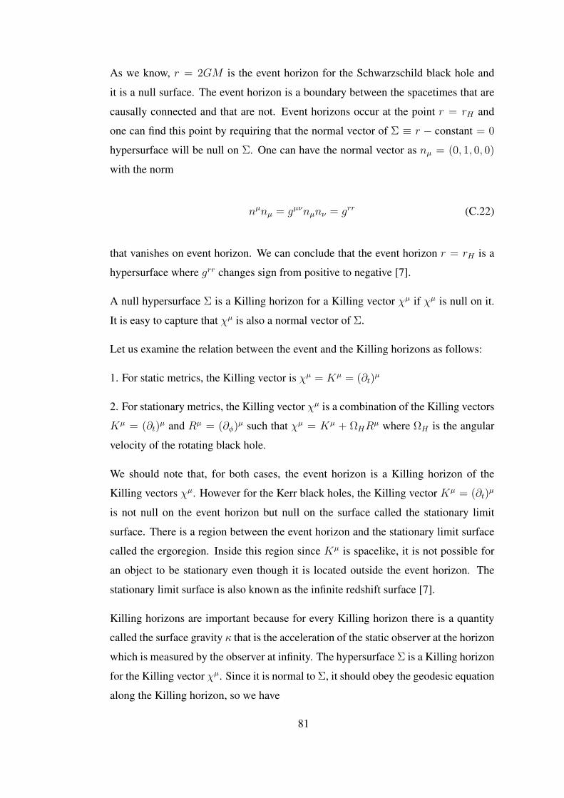
As we know, r = 2GM is the event horizon for the Schwarzschild black hole and
it is a null surface. The event horizon is a boundary between the spacetimes that are
causally connected and that are not. Event horizons occur at the point r = rH and
one can find this point by requiring that the normal vector of Σ ≡ r − constant = 0
hypersurface will be null on Σ. One can have the normal vector as nµ = (0, 1, 0, 0)
with the norm
nµnµ = gµνnµnν = grr (C.22)
that vanishes on event horizon. We can conclude that the event horizon r = rH is a
hypersurface where grr changes sign from positive to negative [7].
A null hypersurface Σ is a Killing horizon for a Killing vector χµ if χµ is null on it.
It is easy to capture that χµ is also a normal vector of Σ.
Let us examine the relation between the event and the Killing horizons as follows:
1. For static metrics, the Killing vector is χµ = Kµ = (∂t)µ
2. For stationary metrics, the Killing vector χµ is a combination of the Killing vectors
Kµ = (∂t)µ and Rµ = (∂φ)µ such that χµ = Kµ + ΩHR
µ where ΩH is the angular
velocity of the rotating black hole.
We should note that, for both cases, the event horizon is a Killing horizon of the
Killing vectors χµ. However for the Kerr black holes, the Killing vector Kµ = (∂t)µ
is not null on the event horizon but null on the surface called the stationary limit
surface. There is a region between the event horizon and the stationary limit surface
called the ergoregion. Inside this region since Kµ is spacelike, it is not possible for
an object to be stationary even though it is located outside the event horizon. The
stationary limit surface is also known as the infinite redshift surface [7].
Killing horizons are important because for every Killing horizon there is a quantity
called the surface gravity κ that is the acceleration of the static observer at the horizon
which is measured by the observer at infinity. The hypersurface Σ is a Killing horizon
for the Killing vector χµ. Since it is normal to Σ, it should obey the geodesic equation
along the Killing horizon, so we have
81

χµ∇µχν = −κχν . (C.23)
The RHS is there because the geodesic equation may not be affinely parametrized.
By using the Killing’s equation and the equation χ[µ∇νχσ ] = 0, one can rewrite the
equation (C.23) as
κ2 = −1
2(∇µχν)(∇µχν)|Σ (C.24)
where Σ represents the horizon [7] .
We already calculated the surface gravity κ by using the particle motion. For Kerr
spacetime, the above formula is useful.
C.2.2 Gravitational Redshift
The gravitational redshift is one of the classical tests of General Relativity. It shows
how the photons gain or lose energy depending on whether they fall or rise in a grav-
itational field. Let us explain how the gravity redshifts the wavelength of the photon.
Consider two static observers A and B such that A sends out light with frequency νA
and the observer B receives it with the frequency νB. We demand that observers are
static since we want to exclude the effects of Doppler-like shifts [7, 46, 73, 74]. We
are sure that both observers agree on the number of pulses they send and receive with
respect to their proper times. Mathematically this leads us to
νAdτA = νBdτB, (C.25)
We know that observers are static hence dr, dφ, dθ vanish and the equation ds2 =
−f(r)dt2 = −dτ 2 leads us to
νAνB
=dτBdτA
=
√|g00(rB)||g00(rA)|
. (C.26)
Since the energy is E = hν we can write the above equation in the form of
EBEA
=
√|g00(rA)||g00(rB)|
. (C.27)
82
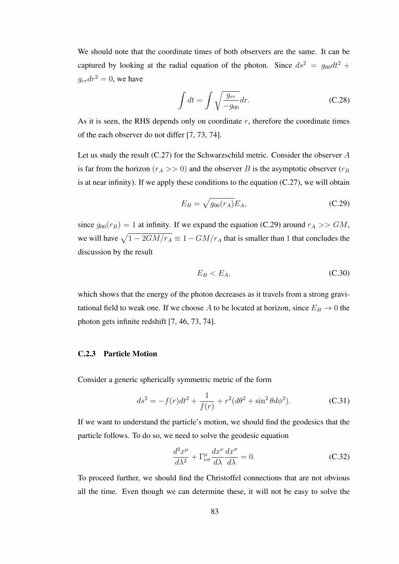
We should note that the coordinate times of both observers are the same. It can be
captured by looking at the radial equation of the photon. Since ds2 = g00dt2 +
grrdr2 = 0, we have ∫
dt =
∫ √grr−g00
dr. (C.28)
As it is seen, the RHS depends only on coordinate r, therefore the coordinate times
of the each observer do not differ [7, 73, 74].
Let us study the result (C.27) for the Schwarzschild metric. Consider the observer A
is far from the horizon (rA >> 0) and the observer B is the asymptotic observer (rB
is at near infinity). If we apply these conditions to the equation (C.27), we will obtain
EB =√g00(rA)EA, (C.29)
since g00(rB) = 1 at infinity. If we expand the equation (C.29) around rA >> GM ,
we will have√
1− 2GM/rA ≡ 1−GM/rA that is smaller than 1 that concludes the
discussion by the result
EB < EA, (C.30)
which shows that the energy of the photon decreases as it travels from a strong gravi-
tational field to weak one. If we choose A to be located at horizon, since EB → 0 the
photon gets infinite redshift [7, 46, 73, 74].
C.2.3 Particle Motion
Consider a generic spherically symmetric metric of the form
ds2 = −f(r)dt2 +1
f(r)+ r2(dθ2 + sin2 θdφ2). (C.31)
If we want to understand the particle’s motion, we should find the geodesics that the
particle follows. To do so, we need to solve the geodesic equation
d2xµ
dλ2+ Γµνσ
dxν
dλ
dxσ
dλ= 0. (C.32)
To proceed further, we should find the Christoffel connections that are not obvious
all the time. Even though we can determine these, it will not be easy to solve the
83

geodesic equation. If the symmetries of the spacetime exist, then we can use them to
determine the particle motion instead of solving the equation C.32. In the Appendix
(B), we already determined the symmetries of a spherically symmetric, static metric
that (C.31) also obeys and obtained the conserved quantities E and L. By using
these quantities as well as the normalization of the four-velocity vector u2 = −1 for
masssive and u2 = 0 for massless particles, we can have the following equations:
r2 = E2 − f(r)− L2f(r)
r2for massive particles, (C.33)
r2 = E2 − L2f(r)
r2for massless particles, (C.34)
where r =d
dλwhere λ is not an affine parameter for the massless case. We should
also note that for the massive case, the quantities E and L represent the energy and
angular momentum per unit mass.
Let us study this to find the geodesics of the Schwarzschild black hole. For this case,
one can write the geodesic equation as
d2t
dλ2+
2GM
r(r − 2GM)
dr
dλ
dt
dλ= 0, (C.35)
d2r
dλ2+GM
r3(r − 2GM)(
dt
dλ)2 − 2GM
r(r − 2GM)
dr
dλ(dr
dλ)2
−(r − 2GM)[(dθ
dλ)2 + sin2 θ(
dφ
dλ)2]
= 0, (C.36)
d2θ
dλ2+
2
r
dr
dλ
dθ
dλ− sin θ cos θ(
dφ
dλ)2 = 0, (C.37)
d2φ
dλ2
+2
r
dr
dλ
dφ
dλ+ 2
cos θ
sin θ
dθ
dλ
dφ
dλ= 0, (C.38)
that are obtained after the proper Christoffel connections [7]. Instead of dealing with
these complicated equations, we can use the symmetries and the conserved quantities
of the Schwarzschild solution. If one puts f(r) = 1 − 2GMr
in the equation (C.33),
then the result would be
r2 = E2 −(1− 2GM
r
)(1 +
L2
r2
)= E2 − V (r) for massive particles, (C.39)
r2 = E2 − L2
r2
(1− 2GM
r
)= E2 − V (r) for massless particles. (C.40)
Also, to determine the orbits of the particle, one should focus on the potential V (r)
84

[7], [74, 76]. If we rewrite the equation (C.39) in the form
r2 = E2 − 1 +2GM
r− L2
r2+
2GML2
r2, (C.41)
where E = 1 represents the rest mass energy of the particle when it is at rest at
infinity, the third term looks like the centrifugal force. Up to now, we are familiar
with these terms from Newtonian mechanics, however the last term is new and it is
the characteristic of the Genereal Relativity. The explanation of the light bending and
the perihelion precession of Mercury follows from this term. The effect of this term
becomes important at distances near the horizon where it can be comparable with the
centrifugal force term [46].
C.2.4 Radial fall of a massive particle
Consider a particle falling radially into a Schwarzschild black hole. Since it is falling
radially, φ = 0 therefore its angular momentum L vanishes. If we apply these results
to radial equation C.41 and use the equation B.24 we have
dr
dτ=(E2 − 1 +
2GM
r
)1/2, (C.42)
dt
dτ= E
(1− 2GM
r
)−1. (C.43)
It is easy to see that the derivative of the equation C.42 with respect to τ and then take
the Newtonian limit τ ≈ t gives
d2r
dt2≈ −GM
r2, (C.44)
which is nothing but the Newtonian gravity [46, 73, 74, 77].
Let us finalize this discussion by determining how long it takes for a particle to reach
the horizon. Assume that initially the paritcle is at some point r0 and if we integrate
the radial equation (C.42), we will have∫dτ = −
∫ 2GM
r0
dr(E2 − 1 +
2GM
r
)1/2, (C.45)
where minus represents that the particle is infalling. Since the integral is finite, the
particle reaches the horizon in a finite proper time. However for an observer at infinity,
85

this is not the case. To find the corresponding time, we should find the expression ofdr
dtthat can be captured by combining the equations (C.42) and (C.43) that gives,
∫dt =
∫ 2GM
r0
Edr(1− 2GM
r
)(E2 − 1 +
2GM
r
)1/2, (C.46)
which diverges logarithmically. Hence for the observer at infinity, it takes infinite
coordinate time for the particle to reach the horizon [46, 73, 74, 77].
86
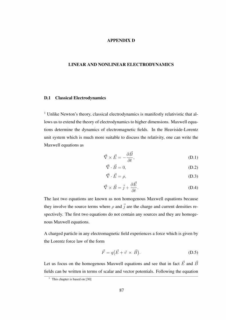
APPENDIX D
LINEAR AND NONLINEAR ELECTRODYNAMICS
D.1 Classical Electrodynamics
1 Unlike Newton’s theory, classical electrodynamics is manifestly relativistic that al-
lows us to extend the theory of electrodynamics to higher dimensions. Maxwell equa-
tions determine the dynamics of electromagnetic fields. In the Heaviside-Lorentz
unit system which is much more suitable to discuss the relativity, one can write the
Maxwell equations as
~∇× ~E = −∂~B
∂t, (D.1)
~∇ · ~B = 0, (D.2)
~∇ · ~E = ρ, (D.3)
~∇× ~B = ~j +∂ ~E
∂t. (D.4)
The last two equations are known as non homogenous Maxwell equations because
they involve the source terms where ρ and ~j are the charge and current densities re-
spectively. The first two equations do not contain any sources and they are homoge-
nous Maxwell equations.
A charged particle in any electromagnetic field experiences a force which is given by
the Lorentz force law of the form
~F = q(~E + ~v × ~B
). (D.5)
Let us focus on the homogenous Maxwell equations and see that in fact ~E and ~B
fields can be written in terms of scalar and vector potentials. Following the equation1 This chapter is based on [30]
87
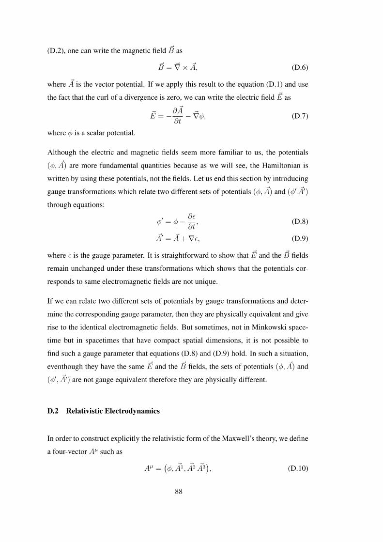
(D.2), one can write the magnetic field ~B as
~B = ~∇× ~A, (D.6)
where ~A is the vector potential. If we apply this result to the equation (D.1) and use
the fact that the curl of a divergence is zero, we can write the electric field ~E as
~E = −∂~A
∂t− ~∇φ, (D.7)
where φ is a scalar potential.
Although the electric and magnetic fields seem more familiar to us, the potentials
(φ, ~A) are more fundamental quantities because as we will see, the Hamiltonian is
written by using these potentials, not the fields. Let us end this section by introducing
gauge transformations which relate two different sets of potentials (φ, ~A) and (φ′ ~A′)
through equations:
φ′ = φ− ∂ε
∂t, (D.8)
~A′ = ~A+∇ε, (D.9)
where ε is the gauge parameter. It is straightforward to show that ~E and the ~B fields
remain unchanged under these transformations which shows that the potentials cor-
responds to same electromagnetic fields are not unique.
If we can relate two different sets of potentials by gauge transformations and deter-
mine the corresponding gauge parameter, then they are physically equivalent and give
rise to the identical electromagnetic fields. But sometimes, not in Minkowski space-
time but in spacetimes that have compact spatial dimensions, it is not possible to
find such a gauge parameter that equations (D.8) and (D.9) hold. In such a situation,
eventhough they have the same ~E and the ~B fields, the sets of potentials (φ, ~A) and
(φ′, ~A′) are not gauge equivalent therefore they are physically different.
D.2 Relativistic Electrodynamics
In order to construct explicitly the relativistic form of the Maxwell’s theory, we define
a four-vector Aµ such as
Aµ =(φ, ~A1, ~A2 ~A3
), (D.10)
88
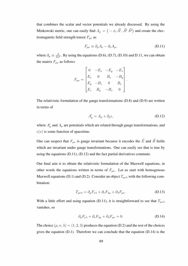
that combines the scalar and vector potentials we already discussed. By using the
Minkowski metric, one can easily find Aµ =(− φ, ~A1, ~A2 ~A3
)and create the elec-
tromagnetic field strength tensor Fµν as
Fµν ≡ ∂µAν − ∂νAµ, (D.11)
where ∂µ ≡ ∂∂xµ
. By using the equations (D.6), (D.7), (D.10) and D.11, we can obtain
the matrix Fµν as follows
Fµν =
0 −Ex −Ey −EzEx 0 Bz −By
Ey −Bz 0 Bx
Ez By −Bx 0
.
The relativistic formulation of the gauge transformations (D.8) and (D.9) are written
in terms of
A′µ = Aµ + ∂µε, (D.12)
where A′µ and Aµ are potentials which are related through gauge transformations, and
ε(x) is some function of spacetime.
One can suspect that Fµν is gauge invariant because it encodes the ~E and ~B fields
which are invariant under gauge transformations. One can easily see that is true by
using the equations (D.11), (D.12) and the fact partial derivatives commute.
Our final aim is to obtain the relativistic formulation of the Maxwell equations, in
other words the equations written in terms of Fµν . Let us start with homogenous
Maxwell equations (D.1) and (D.2). Consider an object Tµνλ with the following com-
bination:
Tµνλ = ∂µFνλ + ∂νFλµ + ∂λFµν . (D.13)
With a little effort and using equation (D.11), it is straightforward to see that Tµνλ
vanishes, so
∂µFνλ + ∂νFλµ + ∂λFµν = 0. (D.14)
The choice (µ, ν, λ) = (1, 2, 3) produces the equation (D.2) and the rest of the choices
gives the equation (D.1). Therefore we can conclude that the equation (D.14) is the
89

relativistic formulation of the homogenous Maxwell equations. We should note that
this equation is known as "Bianchi identity" and it can be also written in terms of a
dual tensor F µν such that
∂µFµν = 0 where F µν ≡ 1
2εµνρσFρσ. (D.15)
The equations (D.3) and (D.4) contain sources so we must introduce a current four-
tensor jµ such that
jµ =(ρ, ~j1, ~j2, ~j3
), (D.16)
where ρ and ~j stands for the charge and current densities respectively. By using the
Minkowski metric and the equation (D.11), it is straightforward to obtain F µν as a
matrix
F µν =
0 Ex Ey Ez
−Ex 0 Bz −By
−Ey −Bz 0 Bx
−Ez By −Bx 0
.So we have,
∂νFµν = jµ, (D.17)
Therefore the equations (D.15) and eqD.17 are precisely the relativistic Maxwell
equaitons.
We should note that these equations are valid in any dimensions. All we have to do
is to define the Lorentz vector Aµ as Aµ =(φ, ~A
)where ~A is the (D − 1) spatial
dimensional vector potential. We should note that in generic dimensions, definition
of F µν changes.
D.3 Non-linear and Born-Infeld Electrodynamıcs
D.3.1 The non-linear electrodynamics
How can we describe the electromagnetism in the presence of materials? We are
sure that the original equations (D.1) -(D.4) are still valid but we are also aware that
they need some modifications. These modifications are necessary due to the materials
90
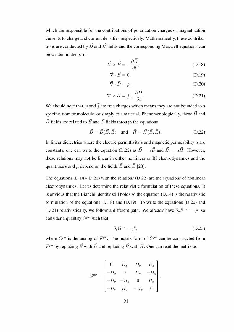
which are responsible for the contributions of polarization charges or magnetization
currents to charge and current densities respectively. Mathematically, these contribu-
tions are conducted by ~D and ~H fields and the corresponding Maxwell equations can
be written in the form
~∇× ~E = −∂~B
∂t, (D.18)
~∇ · ~B = 0, (D.19)
~∇ · ~D = ρ, (D.20)
~∇× ~H = ~j +∂ ~D
∂t. (D.21)
We should note that, ρ and ~j are free charges which means they are not bounded to a
specific atom or molecule, or simply to a material. Phenomenologically, these ~D and~H fields are related to ~E and ~B fields through the equations
~D = ~D( ~B, ~E) and ~H = ~H( ~B, ~E). (D.22)
In linear dielectrics where the electric permittivity ε and magnetic permeability µ are
constants, one can write the equation (D.22) as ~D = ε ~E and ~B = µ ~H . However,
these relations may not be linear in either nonlinear or BI electrodynamics and the
quantities ε and µ depend on the fields ~E and ~B [28].
The equations (D.18)-(D.21) with the relations (D.22) are the equations of nonlinear
electrodynamics. Let us determine the relativistic formulation of these equations. It
is obvious that the Bianchi identity still holds so the equation (D.14) is the relativistic
formulation of the equations (D.18) and (D.19). To write the equations (D.20) and
(D.21) relativistically, we follow a different path. We already have ∂νF µν = jµ so
consider a quantity Gµν such that
∂νGµν = jµ, (D.23)
where Gµν is the analog of F µν . The matrix form of Gµν can be constructed from
F µν by replacing ~E with ~D and replacing ~B with ~H . One can read the matrix as
Gµν =
0 Dx Dy Dz
−Dx 0 Hz −Hy
−Dy −Hz 0 Hx
−Dz Hy −Hx 0
.
91
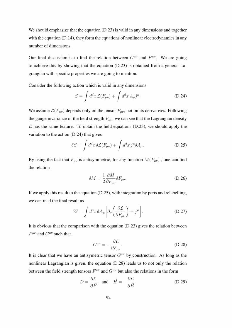
We should emphasize that the equation (D.23) is valid in any dimensions and together
with the equation (D.14), they form the equations of nonlinear electrodynamics in any
number of dimensions.
Our final discussion is to find the relation between Gµν and F µν . We are going
to achieve this by showing that the equation (D.23) is obtained from a general La-
grangian with specific properties we are going to mention.
Consider the following action which is valid in any dimensions:
S =
∫ddxL(Fµν) +
∫ddxAµj
µ. (D.24)
We assume L(Fµν) depends only on the tensor Fµν , not on its derivatives. Following
the gauge invariance of the field strength Fµν , we can see that the Lagrangian density
L has the same feature. To obtain the field equations (D.23), we should apply the
variation to the action (D.24) that gives
δS =
∫ddx δL(Fµν) +
∫ddx jµδAµ. (D.25)
By using the fact that Fµν is antisymmetric, for any function M(Fµν) , one can find
the relation
δM =1
2
∂M
∂FµνδFµν . (D.26)
If we apply this result to the equation (D.25), with integration by parts and relabelling,
we can read the final result as
δS =
∫ddx δAµ
[∂ν
(∂L∂Fµν
)+ jµ
]. (D.27)
It is obvious that the comparison with the equation (D.23) gives the relation between
F µν and Gµν such that
Gµν = − ∂L∂Fµν
. (D.28)
It is clear that we have an antisymetric tensor Gµν by construction. As long as the
nonlinear Lagrangian is given, the equation (D.28) leads us to not only the relation
between the field strength tensors F µν and Gµν but also the relations in the form
~D =∂L∂ ~E
and ~H = −∂L∂ ~B
. (D.29)
92
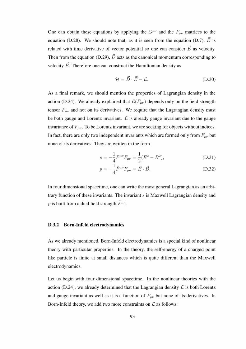
One can obtain these equations by applying the Gµν and the Fµν matrices to the
equation (D.28). We should note that, as it is seen from the equation (D.7), ~E is
related with time derivative of vector potential so one can consider ~E as velocity.
Then from the equation (D.29), ~D acts as the canonical momentum corresponding to
velocity ~E. Therefore one can construct the Hamiltonian density as
H = ~D · ~E − L. (D.30)
As a final remark, we should mention the properties of Lagrangian density in the
action (D.24). We already explained that L(Fµν) depends only on the field strength
tensor Fµν and not on its derivatives. We require that the Lagrangian density must
be both gauge and Lorentz invariant. L is already gauge invariant due to the gauge
invariance of Fµν . To be Lorentz invariant, we are seeking for objects without indices.
In fact, there are only two independent invariants which are formed only from Fµν but
none of its derivatives. They are written in the form
s = −1
4F µνFµν =
1
2(E2 −B2), (D.31)
p = −1
4F µνFµν = ~E · ~B. (D.32)
In four dimensional spacetime, one can write the most general Lagrangian as an arbi-
trary function of these invariants. The invariant s is Maxwell Lagrangian density and
p is built from a dual field strength F µν .
D.3.2 Born-Infeld electrodynamics
As we already mentioned, Born-Infeld electrodynamics is a special kind of nonlinear
theory with particular properties. In the theory, the self-energy of a charged point
like particle is finite at small distances which is quite different than the Maxwell
electrodynamics.
Let us begin with four dimensional spacetime. In the nonlinear theories with the
action (D.24), we already determined that the Lagrangian density L is both Lorentz
and gauge invariant as well as it is a function of Fµν but none of its derivatives. In
Born-Infeld theory, we add two more constraints on L as follows:
93
1. The vanishing magnetic field ~B = 0 should lead to the maximal electric field ~Emax
2. For small electromagnetic fields, L(Fµν) should produce to Maxwell Lagrangian.
The maximal electric field is borrowed from string theory in which the critical electric
field is written as Ecrit = 1/2πα′ ≡ b. This condition on electric field was considered
necessary by Born and Infeld to get a finite self energy of the particle. To proceed
further, we should find a way to impose these conditions to the Lagrangian. In Special
Relativity, the constraint on the velocity is given in the point particle Lagrangian as
L = −m√
1− v2. (D.33)
This gives a hint on how we can impose the condition Ecrit ≤ b to the Lagrangian.
For an expression with the Lorentz invariant s only, we have
L = −b2
√1− ( ~E2 − ~B2)
b2+ b2. (D.34)
It is easy to capture that this Lagrangian (D.34) satisfies the requirements. Let us
introduce the Born-Infeld Lagrangian in four dimensional spacetime
LBI = −b2
√1− ( ~E2 − ~B2)
b2− ( ~E · ~B)2
b4+ b2. (D.35)
It is easily seen that the Lagrangian LBI satisfies the constraints we demand. When~B = 0, E ≤ b is satisfied. Also for small fields, it reduces to LM =
1
2(E2 −B2).
The crucial point about Born-Infeld Lagrangian is that it can be written in terms of a
determinant which is valid in any dimensions as opposed to (D.35):
L = −b2
√− det
(ηµν +
1
bFµν
)+ b2. (D.36)
We can easily show that the equations (D.35) and (D.36) are equal to each other in
four dimensions. To do this, we should show that the Lagrangian density in (D.36)
is Lorentz invariant. To make calculations easier, let us take b = 1 and write the
equation (D.36) in terms of
L = −
√− det
(ηµν + Fµν
)+ 1. (D.37)
94
It is straightforward to see that the determinants of two vectors M and M with com-
ponents Mµν and Mµν respectively are equivalent. If we apply this to the inside of
the equation (D.37), we get
det(η + F ) = det(η + F ), (D.38)
where the η and F are matrices with components ηµν and F µν respectively. We are
done when we prove the Lorentz invariance of the det(η + F ). To show this, all
we need to show is that det(η + F ) is unchanged under the Lorentz transformations
which can be written as
η′µν + F ′µν = ΛµρΛν
σ(ηρσ + F ρσ), (D.39)
η′ + F ′ = Λ(η + F )ΛT , (D.40)
⇒ det(η′ + F ′) = det(η + F ), (D.41)
which proves the Lorentz invariance of the equation (D.37). To see the equivalence
of the Lagrangians (D.36) and (D.37), we can write the latter in terms of
det(η + F ) = det(η(1 + ηF )) = − det(1 + ηF ), (D.42)
where we used the fact that det η = −1. By following the exact calculation, one can
show that the determinat of the matrix 1 + ηF in four dimensional spacetime reduces
to the result (D.35).
Let us end this chapter by showing that the self energy of a point particle is finite in
Born-Infeld electrodynamics as opposed to Maxwell theory. To simplify the calcula-
tions, we can use the LBI in (D.35) with the assumption that ~B = 0. Then we read
the Lagrangian density as
L = −b2
√1−
~E2
b2+ b2. (D.43)
Since we are given the Lagrangian, we can immediately use the equation (D.29) to
find the ~D-field in terms of
~D =~E√
1− E2/b2. (D.44)
95
If we solve the above equation for ~E then the result
E2 = b2
(D2
D2 + b2
)and ~E =
~D√1 +D2/b2
, (D.45)
from where we see that the electric field is bounded by b as expected. By calculating
its magnitude, one can see that there is no bound on D. In fact, it should be infinitely
large to have E = b. If we apply this electric field to the equation (D.43), we can the
Lagrangian density as
L = − b2√1 +D2/b2
+ b2. (D.46)
Then the Hamiltonian density can be given as
H = b2
√1 +
D2
b2− b2. (D.47)
This is the Born-Infeld energy density which is valid in any number of dimensions
when ~B = 0. We are going to use it to find the self energy of a point particle in
Maxwell and Born-Infeld theories.
In Maxwell theory, energy densityH = ~D· ~E−L is proportional toE·D = E2 and we
know that E is a function like 1/r2. Therefore the integral∫d3xE2 is proportional
with 1/r2 which is not finite for small r. It shows that the energy of a point particle
is infinite in Maxwell theory.
In Born-Infeld theory, the energy density is given by the equation (D.47) that takes
the form
H ≈ bD = EcritD, (D.48)
for large D fields. Therefore the integrand∫d3xEcritD is proportional to dr that
converges.
Let us summarize what we obtained. We showed that the energy density in Maxwell
theory is proportional to E ·D. Since D and E are functions of r−2 the term d3xE2
will diverge for small fields. On the other hand, the energy density in Born-Infeld
theory is proportional to bD that leads a convergent integrand for large fields and
small distances.
96
APPENDIX E
A BRIEF LOOK AT BLACK HOLE ENTROPY IN BORN-INFELD
GRAVITY
In chapter 3 we studied the entropy of the de Sitter space for generic gravity and did
not discuss black hole entropy (except for the n = 2+1 dimensions). The main reason
for this is that the BI theories studied here are quite recent and no exact black hole
type solutions have been found for these theories. The only relevant work up to now is
[65] where perturbative solutions were constructed. But for the sake of completeness
and as an initial estimate to what happens to the entropy of Schwarzschild-Tangherlini
black holes in the BI gravity, let us carry out the following computation which should
be considered as a preliminary work. To be specific, let us take the Lagrangian (3.40)
which reads
L =2
γ
(f(Rµναβ)n/2 − λ0 − 1
), (E.1)
where
f(Rµναβ) = 1 + pR + uR2µναβ − 4uR2
µν + (u− v)R2, (E.2)
with the coefficients
p =γ
n, u =
γ2(n− 1)2
4n(n− 2)(n− 3), v =
γ2(n− 2)
4n2. (E.3)
With the help of (3.29), the derivative of the Lagrangian with respect to the Riemann
tensor can be found as
∂L∂Rabcd
=n
γf(Rµναβ)
n−22
[[p+ 2(u− v)R
]gc[agb]d + 2uRabcd
−4u(ga[cRd]b − gb[cRd]a
) ]. (E.4)
97
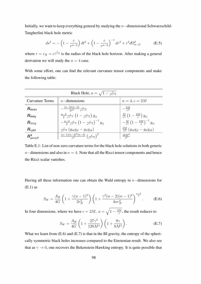
Initially, we want to keep everything general by studying the n−dimensional Schwarzschild-
Tangherlini black hole metric
ds2 = −(
1− c
rn−3
)dt2 +
(1− c
rn−3
)−1
dr2 + r2dΩ2n−2, (E.5)
where r = rH = c1
n−3 is the radius of the black hole horizon. After making a general
derivation we will study the n = 4 case.
With some effort, one can find the relevant curvature tensor components and make
the following table:
Black Hole, a =√
1− crn−3
Curvature Terms n−dimensions n = 4, c = 2M
R0101 − (n−2)(n−3)2r2
crn−3 −2M
r3
R0i0jn−3
2c
rn−1
(1− c
rn−3
)gij
Mr3
(1− 2M
r
)gij
R1i1j −n−32
crn−1
(1− c
rn−3
)−1gij −M
r3
(1− 2M
r
)−1gij
Rijklc
rn−1 (gikgjl − gilgjk) 2Mr3
(gikgjl − gilgjk)
R2µναβ
(n−1)(n−2)2(n−3)r4
(c
rn−3
)2 48M2
r6
Table E.1: List of non-zero curvature terms for the black hole solutions in both generic
n−dimensions and also in n = 4. Note that all the Ricci tensor components and hence
the Ricci scalar vanishes.
Having all these information one can obtain the Wald entropy in n−dimensions for
(E.1) as
SW =AH4G
(1 +
γ(n− 1)2
2r2H
)(1 +
γ2(n− 2)(n− 1)3
4nr4H
)n−22
. (E.6)
In four dimensions, where we have c = 2M, a =√
1− 2Mr
, the result reduces to
SW =AH4G
(1 +
27γ2
128M4
)(1 +
9γ
8M2
). (E.7)
What we learn from (E.6) and (E.7) is that in the BI gravity, the entropy of the spheri-
cally symmetric black holes increases compared to the Einstenian result. We also see
that as γ → 0, one recovers the Bekenstein-Hawking entropy. It is quite possible that
98
one can write SW as the geometric entropy with a modified gravitational constant.
But for this to work out, we need the exact black hole solutions in the BI gravity
which we currently lack.
99

100
CURRICULUM VITAE
PERSONAL INFORMATION
Surname, Name: Özen, Gökçen Deniz
Nationality: Turkish
Date and Place of Birth: 22.02.1988, Bursa
E-mail: [email protected]
EDUCATION
• M. Sc. in Physics, (2011-2014),
Middle East Technical University,
Advisor: Prof. Dr. Bayram Tekin
Thesis: Gravitomagnetism in General Relativity
and Massive Gravity
• Scientific Preparation in Physics, (2010-2011),
Middle East Technical University,
• B. Sc. in Mathematics, (2006-2010),
Middle East Technical University,
PROFESSIONAL EXPERIENCE
• Research assistant in Physics Department of Middle East Technical University,
2013-2021.
• Guest researcher in Utrecht University (with scholarship), 2019-2020.
101

• Researcher in the Scientific and Technological Research Council of Turkey
(TUBITAK) under project 109E233, 2010-2013.
HONORS AND AWARDS
• Scholarship from TUBITAK 2214 A International Research Fellowship Pro-
gramme for PhD Students, 2019-2020.
PUBLICATIONS
1. G.D. Ozen, S. Kürekçi and B. Tekin, " Entropy in Born-Infeld Gravity", Phys. Rev.
D 96, 124038 (2017).
2. H. D. Karaca, G. D. Özen, C. Kasnakoglu, "A Nonlinear Dynamical Modeling and
Control Method for the Vorticity Control of the Flow Past a Circular Cylinder", Inter-
national Journal of Materials, Mechanics and Manufacturing, 1(4): 324-346, (2013),
DOI: 10.7763/IJMMM.2013.V1.74.
3. O. Durmaz, H. D. Karaca, G. D. Ozen, C. Kasnakoglu, D. F. Kurtulus, "Dynamical
modelling of the flow over a flapping wing using proper orthogonal decomposition
and system identification techniques," Mathematical and Computer Modelling of Dy-
namical Systems, 19(2), 133-158, (2013), DOI: 10.1080/13873954.2012.705859.
Summer Schools
Summer School on Superstring Theory and Related Topics, 24 August-04 September
2020, ICTP.
School on Geometry and Gravity, 15-26 July 2019, ICTP
Presentations
• Title of the talk : Entropy Calculation in Born-Infeld Type Gravity Theories, -
Poster presentation, School on Geometry and Gravity, 15-26 July 2019, ICTP.
102

• Title of the talk : Entropy in Born-Infeld Gravity, - 17. Quantization, Dualities
and Integrable Systems, 20-22 April 2019, Denizli.
103
Top Related